Geometry - Home - Springer D. Bremner, K. Fukuda, and A. Marzetta 1. Introduction...

Discrete Comput Geom 20:333–357 (1998) Discrete & Computational

Geometry© 1998 Springer-Verlag New York Inc.

Primal–Dual Methods for Vertex and Facet Enumeration∗

D. Bremner,1 K. Fukuda,2,3 and A. Marzetta4

1Department of Mathematics, University of Washington,Seattle, WA 98195, [email protected]

2Department of Mathematics,Swiss Federal Institute of Technology,Lausanne, Switzerland

3Institute for Operations Research,Swiss Federal Institute of Technology,Zurich, [email protected]

4Institute for Theoretical Computer Science,Swiss Federal Institute of Technology,Zurich, [email protected]

Abstract. Every convex polytope can be represented as the intersection of a finite set ofhalfspaces and as the convex hull of its vertices. Transforming from the halfspace (resp.vertex) to the vertex (resp. halfspace) representation is calledvertex enumeration(resp.facetenumeration). An open question is whether there is an algorithm for these two problems(equivalent by geometric duality) that is polynomial in the input size and the output size.In this paper we extend the known polynomially solvable classes of polytopes by lookingat the dual problems. Thedual problem of a vertex (resp. facet) enumeration problem isthe facet (resp. vertex) enumeration problem for the same polytope where the input andoutput are simply interchanged. For a particular class of polytopes and a fixed algorithm,one transformation may be much easier than its dual. In this paper we propose a new classof algorithms that take advantage of this phenomenon. Loosely speaking,primal–dualalgorithms use a solution to the easy direction as an oracle to help solve the seemingly harddirection.

∗ The first author’s research was supported by NSERC Canada, FCAR Qu´ebec, and the J.W. McConnellFoundation.

334 D. Bremner, K. Fukuda, and A. Marzetta

1. Introduction

A polytopeis the bounded intersection of a finite set of halfspaces inRd. Theverticesof apolytope are those feasible points that do not lie in the interior of a line segment betweentwo other feasible points. Every polytopeP can be represented as the intersection of anonredundant set of halfspacesH(P) and as the convex hull of its verticesV(P). Theproblem of transforming fromH(P) toV(P) is calledvertex enumeration; transformingfrom V(P) toH(P) is calledfacet enumerationor convex hull.

An algorithm is said to bepolynomialif the time to solve any instance is boundedabove by a polynomial in the size of input and output. We consider the input (resp.output) size to be the number of real (or rational) numbers needed to represent theinput (resp. output); in particular we do not consider the dimension to be a constant. Weassume each single arithmetic operation takes a constant amount of time.1 A successivelypolynomial algorithmis one whosekth output is generated in time polynomial ink andthe input sizes, for eachk less than or equal to the cardinality of output. Clearly, everysuccessively polynomial algorithm is a polynomial algorithm. We assume that a polytopeis full-dimensional and contains the origin in its interior; under these conditions2 vertexenumeration and facet enumeration are polynomially equivalent, that is, the existence ofa polynomial algorithm for one problem implies the same for the other problem. Severalpolynomial algorithms (see, e.g., [3], [6], [7], [9], [17], and [18]) are known under strongassumptions of nondegeneracy, which restrict input polytopes to be simple in the case ofvertex enumeration and simplicial in the case of facet enumeration. However, it is openwhether there exists a polynomial algorithm in general.

In this paper we extend the known polynomially solvable classes by looking at thedual problems. Thedual problem of a vertex (resp. facet) enumeration problem is thefacet (resp. vertex) enumeration problem for the same polytope where the input andoutput are simply interchanged. For a particular class of polytopes and a fixed algorithm,one transformation may be much easier than its dual. One might be tempted to explainthis possible asymmetry by observing that the standard nondegeneracy assumption isnot self-dual. Are the dual problems of nondegenerate vertex (facet) enumeration prob-lems harder? More generally, are the complexities of the primal and the dual problemdistinct?

Here we show in a certain sense that the primal and dual problems are of the samecomplexity. More precisely, we show the following theorem: if there is a successivelypolynomial algorithm for the vertex (resp. facet) enumeration problem for a hereditaryclass of problems, then there is a successively polynomial algorithm for the facet (resp.vertex) enumeration problem for the same class, where a hereditary class contains allsubproblems of any instance in the class. We propose a new class of algorithms that takeadvantage of this phenomenon. Loosely speaking,primal–dualalgorithms use a solutionto the easy direction as an oracle to help solve the seemingly hard direction.

1 This assumption is merely to simplify our discussion. One can easily analyze the complexity of an algo-rithm in our primal–dual framework for the binary representation model and in general its binary complexitydepends only on that of the associated “base” algorithm.

2 We discuss these assumptions further in Section 2.2.

Primal–Dual Methods for Vertex and Facet Enumeration 335

From this general result relating the complexity of the primal and dual problems, andknown polynomial algorithms for the primal-nondegenerate case, we arrive at a polyno-mial algorithm for vertex enumeration for simplicial polytopes and facet enumeration forsimple polytopes. We then show how to refine this algorithm to yield an algorithm withtime complexity competitive with the algorithms known for the primal-nondegeneratecase.

The only published investigation of the dual-nondegenerate case the authors are awareof is in a paper by Gritzmann and Klee [12]. Their approach, most easily understoodin terms of vertex enumeration, consists of intersecting the constraints with each defin-ing hyperplane and, after removing the redundant constraints, finding the vertices lyingon that facet by some brute-force method. David Avis (private communication) has in-dependently observed that this method can be extended to any polytope whose facetsare simple (or nearly simple) polytopes. The method of Gritzmann and Klee requiressolving O(m2) linear programs (wherem is the number of input halfspaces) to re-move redundant constraints. Our approach does not rely on the polynomial solvabilityof linear programming if an interior point is known (as is always the case for facetenumeration).

Notation

We start by defining some notation. Recall thatH(P) (resp.V(P)) is the nonredundanthalfspace (resp. vertex) description ofP. We usem for |H(P)|, n for |V(P)|, andd forthe dimension dimP. The facets ofP are the intersection of the bounding hyperplanes ofH(P)with P. We useO (Ok) and1 (1k) to denote the vector of all zeros (of lengthk) andall ones (of lengthk), respectively. We treat sets of points and matrices interchangeablywhere convenient; the rows of a matrix are the elements of the corresponding set. Given(row or column) vectorsa andb, we useab to denote the inner product ofa andb. Sincewe assume the origin is in the interior of each polytope, each facet defining inequalitycan be written ashx ≤ 1 for some vectorh. For a vectorh, we useh+, h−, andh0

to denote the set of pointsx such thathx ≤ 1, hx > 1, andhx = 1, respectively. Wesometimes identify the halfspaceh+ with the associated inequalityhx ≤ 1 where there isno danger of confusion. We useP(H) to denote the polyhedron{x | Hx ≤ 1}. Similarlywe useH(P) to mean the matrixH whereP = {x | Hx ≤ 1}. For a set of pointsVwe useH(V) to meanH(convV); similarly for a set of halfspacesH , we useV(H)to meanV(P(H)). We say thath+ is valid for a set of pointsX (or hx ≤ 1 is avalidinequality) if X ⊆ h+. We make extensive use of duality of convex polytopes in whatfollows. Theproper facesof a convex polytope are the intersection of some set of facets.By adding the twoimproper faces, the polytope itself and the empty set, the faces form alattice ordered by inclusion. Two polytopes are said to becombinatorially equivalentiftheir face lattices are isomorphic anddual if their face lattices are anti-isomorphic (i.e.,isomorphic with the direction of inclusion reversed). The following is well known (see,e.g., [5]).

Proposition 1. If P = convX is a polytope such thatO ∈ int P, then Q= {y | Xy≤1} is a polytope dual to P such thatO ∈ int Q.


2. Primal–Dual Algorithms

In this section we consider the relationship between the complexity of the primal prob-lem and the complexity of the dual problem for vertex/facet enumeration. We fix theprimal problem as facet enumeration in the rest of this paper, but the results can also beinterpreted in terms of vertex enumeration. For convenience we assume in this paper thatthe input polytope is full-dimensional and contains the origin as an interior point. Whileit is easy to see this is no loss of generality in the case of facet enumeration, in the caseof vertex enumeration one might need to solve a linear program to find an interior point.We call a family0 of polytopesfacet-hereditaryif for any P ∈ 0, for anyH ′ ⊂ H(P),if⋂

H ′ is bounded, then⋂

H ′ is also in0. The main idea of this paper is summarizedby the following theorem.

Theorem 1. If there is a successively polynomial vertex enumeration algorithm fora facet-hereditary family of polytopes, then there is a successively polynomial facetenumeration algorithm for the same family.

Simple polytopes are not necessarily facet-hereditary, but each simple polytope can beperturbed symbolically or lexicographically onto a combinatorially equivalent polytopewhose facet defining halfspaces are in “general position,” i.e., the arrangement of facetinducing hyperplanes defined by the polytope is simple. The family of polytopes whosefacet inducing halfspaces are in general position is obviously facet-hereditary.

Corollary 1. There is a successively polynomial algorithm for facet enumeration ofsimple polytopes and for vertex enumeration of simplicial polytopes.

Proof of Theorem 1 is constructive, via the correctness of Algorithm 1. Algorithm 1takes as input a setV of points inRd, and a subsetH0 ⊂ H(V) such that

⋂H0 is

bounded. We show below how to compute such a set of halfspaces.At every step of the algorithm we maintain the invariant that convV ⊆ P(Hcur).

When the algorithm terminates, we know thatV(Hcur) ⊆ V . It follows thatP(Hcur) ⊆convV . There are two main steps in this algorithm that we have labeled FindWitness andDeleteVertex. The vertexv ∈ V(Hcur)\V is awitnessin the sense that for any such vertex,there must be a facet ofH(V) not yet discovered whose defining halfspace cuts offv.From the precondition of the theorem there exists a successively polynomial algorithm

Algorithm 1. PrimalDualFacets(V, H0)

Hcur← H0

while ∃v ∈ V(Hcur)\V do FindWitnessFind h ∈ H(V) s.t. v ∈ h− DeleteVertexHcur← Hcur∪ {h}

endwhilereturnHcur.


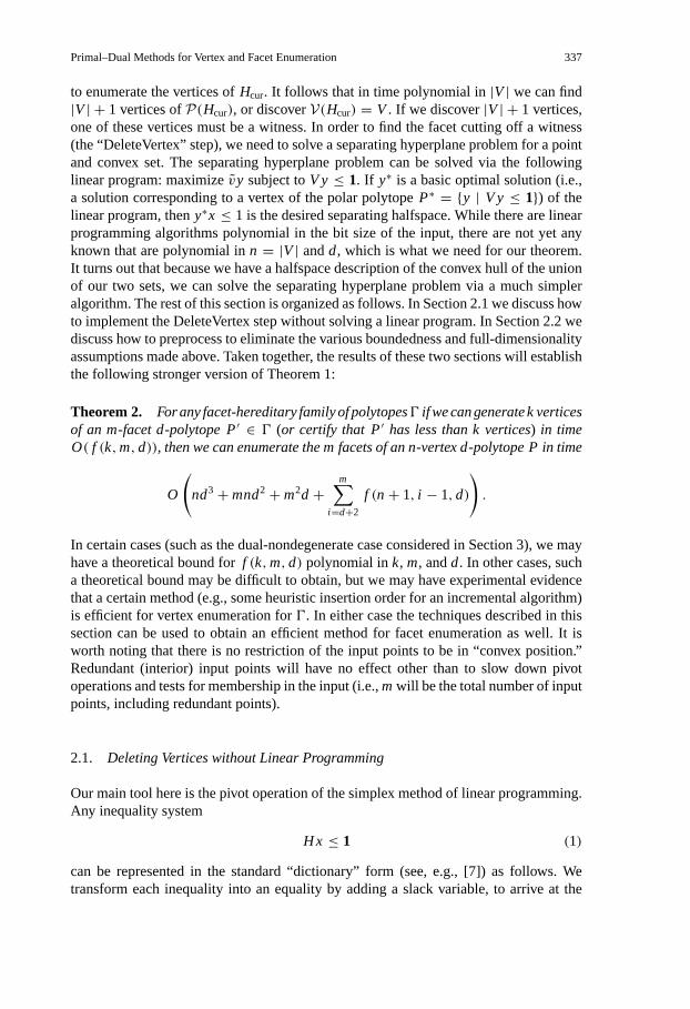
to enumerate the vertices ofHcur. It follows that in time polynomial in|V | we can find|V | + 1 vertices ofP(Hcur), or discoverV(Hcur) = V . If we discover|V | + 1 vertices,one of these vertices must be a witness. In order to find the facet cutting off a witness(the “DeleteVertex” step), we need to solve a separating hyperplane problem for a pointand convex set. The separating hyperplane problem can be solved via the followinglinear program: maximizevy subject toV y ≤ 1. If y∗ is a basic optimal solution (i.e.,a solution corresponding to a vertex of the polar polytopeP∗ = {y | V y ≤ 1}) of thelinear program, theny∗x ≤ 1 is the desired separating halfspace. While there are linearprogramming algorithms polynomial in the bit size of the input, there are not yet anyknown that are polynomial inn = |V | andd, which is what we need for our theorem.It turns out that because we have a halfspace description of the convex hull of the unionof our two sets, we can solve the separating hyperplane problem via a much simpleralgorithm. The rest of this section is organized as follows. In Section 2.1 we discuss howto implement the DeleteVertex step without solving a linear program. In Section 2.2 wediscuss how to preprocess to eliminate the various boundedness and full-dimensionalityassumptions made above. Taken together, the results of these two sections will establishthe following stronger version of Theorem 1:

Theorem 2. For any facet-hereditary family of polytopes0 if we can generate k verticesof an m-facet d-polytope P′ ∈ 0 (or certify that P′ has less than k vertices) in timeO( f (k,m,d)), then we can enumerate the m facets of an n-vertex d-polytope P in time

O

(nd3+mnd2+m2d +

m∑i=d+2

f (n+ 1, i − 1,d)

).

In certain cases (such as the dual-nondegenerate case considered in Section 3), we mayhave a theoretical bound forf (k,m,d) polynomial ink, m, andd. In other cases, sucha theoretical bound may be difficult to obtain, but we may have experimental evidencethat a certain method (e.g., some heuristic insertion order for an incremental algorithm)is efficient for vertex enumeration for0. In either case the techniques described in thissection can be used to obtain an efficient method for facet enumeration as well. It isworth noting that there is no restriction of the input points to be in “convex position.”Redundant (interior) input points will have no effect other than to slow down pivotoperations and tests for membership in the input (i.e.,m will be the total number of inputpoints, including redundant points).

2.1. Deleting Vertices without Linear Programming

Our main tool here is the pivot operation of the simplex method of linear programming.Any inequality system

Hx ≤ 1 (1)

can be represented in the standard “dictionary” form (see, e.g., [7]) as follows. Wetransform each inequality into an equality by adding a slack variable, to arrive at the


following system of linear equations ordictionary:

s= 1− Hx. (2)

More precisely, a dictionary for (1) is a system obtained by solving (2) for some subset ofmslack and original variables (wherem is the row size ofH ). A solution to (2) is feasiblefor (1) if and only ifs ≥ O. In particular, sinceHO < 1, s= 1 is a feasible solution toboth. The variables are naturally partitioned into two sets. The variables appearing onthe left-hand side of a dictionary are calledbasic; those on the right-hand side are calledcobasic. A pivot operation moves between dictionaries by making one cobasic variable(theentering variable) basic and one basic variable (theleaving variable) cobasic.

If we have a feasible point for a polytope and a halfspace description, ind pivotoperations we can find a vertex of the polytope. If we ensure that each pivot does notdecrease a given objective function, then we have the following.

Lemma 1 (Raindrop Algorithm). Given H∈ Rm×d, ω ∈ Rd, andv0 ∈ P(H), in timeO(md2) we can findv ∈ V(H) such thatωv ≥ ωv0.

Proof. We start by translating our system by−v0 so that our initial point is the origin.As a final row to our dictionary we add the the equationz= ωx (theobjective row). Notethat, by construction,x = O is a feasible solution. We start a pivot operation by choosingsome cobasic variablexj to become basic. Depending on the sign of the coefficient ofxj in the objective row, we can always increase or decreasexj without decreasing thevalue ofz. As we change the value ofxj , some of the basic slack variables will decreaseas we get closer to the corresponding hyperplane. By considering ratios of coefficients,we can find one of the first hyperplanes reached. By moving that slack variable to theright-hand side (making it cobasic), and movingxj to the left-hand side, we obtain anew dictionary inO(md) time (see, e.g., [7] for details of the simplex method). We cancontinue this process as long as there is a cobasicx-variable. After exactlyd pivots, allx-variables are basic. It follows that the corresponding basic feasible solution is a vertex(see Fig. 1).

The raindrop algorithm seems to be part of the folklore of Linear Programming; ageneralized version is discussed in [16].

By duality of convex polytopes we have the following.

Fig. 1. The raindrop algorithm.


Fig. 2. Pivoting from a valid inequality to a facet.

Lemma 2 (Dual Raindrop Algorithm). Given V ∈ Rn×d, ω ∈ Rd, and h0 such thatV ⊂ h+0 , in O(nd2) time we can find h∈ H(V) such that hω ≥ h0ω.

Essentially this is the same as the initialization step of a gift-wrapping algorithm (see,e.g., [6] and [18]), except that we are careful that the pointω is on the same side of ourfinal hyperplane as the one we started with. Figure 2 illustrates the rotation dual to thepivot operation in Lemma 1.

We can now show how to implement the DeleteVertex step of Algorithm 1 withoutlinear programming. Abasis Bfor a vertexv ∈ V(H) is a set ofd rows of H suchthat Bv = 1 and rankB = d. We can obviously find a basis in polynomial time; in thepivoting-based algorithms in the following sections we will always be given a basis forv.

Lemma 3 (DeleteVertex). Given V∈ Rn×d, H0 ⊂ H(V), v ∈ V(H0)\V , and a basisB for v, we can find h∈ H(V) such thatv ∈ h− in time O(nd2).

Proof. Let h = (1/d)∑b∈B b. The inequalityhx ≤ 1 is satisfied with equality byvand with strict inequality by everyv ∈ V (sincev is the unique vertex ofP(H0) lyingon h0; see Fig. 3). Letγ = maxv∈V hv. SinceO ∈ int convV , γ > 0. Let h0 = h/γ .The constrainth0x ≤ 1 is valid for convV , buth0v > 1. The lemma then follows fromLemma 2.

Fig. 3. Illustrating the proof of Lemma 3.


If we are not given a basis for the vertexv we wish to cut off, we can use the mean ofthe outward normals of all facets meeting atv in place of the vectorh. This mean vectorcan be computed inO(|H0|d) time.

Corollary 2. Given V∈ Rn×d, H0 ⊂ H(V),andv ∈ V(H0)\V ,we can find h∈ H(V)such thatv ∈ h− in time O(nd2+ |H0|d).

It will prove useful below to be able to find a facet of convV that cuts off a particularextreme ray or direction of unboundedness for our current intermediate polyhedron.

Lemma 4 (DeleteRay). Given V ∈ Rn×d and r ∈ Rd\{O}, in O(nd2) time we canfind h∈ H(V) such that hr> 0.

Proof. The proof is similar to that of Lemma 3. Letγ = maxv∈V r v. SinceO ∈int convV , γ > 0. Let h0 = r/γ . The constrainth0x ≤ 1 is valid for convV , buth0r = (r · r )/γ > 0. By Lemma 2, inO(nd2) time we can computeh ∈ H(V) suchthathr ≥ h0r > 0.

2.2. Preprocessing

We have assumed throughout that the input polytopes are full-dimensional and containthe origin as an interior point. This is polynomially equivalent to assuming that alongwith a halfspace or vertex description ofP, we are given a relative interior point, i.e.,an interior point ofP in aff P. Given a relative interior point, then (either representationof) P can be shifted to contain the origin as an interior point and embedded in a spaceof dimension dimP in O(Nd2) time by elementary matrix operations, whereN is thenumber of input halfspaces or points.

Finding a relative interior point in a set of points requires only the computation of thecentroid. On the other hand, finding a relative interior point of the intersection of a setof halfspacesH requires solving at least one (and no more than|H |) linear programs.Since we are interested here in algorithms polynomial inn, m, andd, and there not yetany such linear programming algorithms, we thus assume that the relative interior pointis given.

In order to initialize Algorithm 1, we need to find some subsetH0 ⊂ H(V) whoseintersection is bounded. We start by showing how to find a subset whose intersection ispointed, i.e., has at least one vertex.

Lemma 5. Given V∈ Rn×d, in O(nd3) time,Algorithm2computes subset H⊂ H(V)such that

⋂H defines a vertex.

Proof. We can compute a parametric representation of the affine subspaceA defined bythe intersection of all hyperplanes found so far inO(d3) time by Gaussian elimination.With each DeleteRay call in Algorithm 2, we find a hyperplane that cuts off some ray inthe previous affine subspace (see Fig. 4). It follows that the dimension ofA decreaseswith every iteration.


Algorithm 2. FindPointedCone

H ← ∅. Er ← x ∈ Rd\{O}.A← Rd.while |H | < d do

h← DeleteRay(Er ,V)H ← H ∪ {h}A← A ∩ h0

Let a andb distinct points inA.Er ← a− b.

endwhilereturnH

We now show how to augment the set of halfspaces computed by Algorithm 2 sothat the intersection of our new set is bounded. To do so, we use a constructive proofof Caratheodory’s theorem. The version we use here is based on that presented byEdmonds [10]. Similar ideas occur in an earlier paper by Klee [14].

Lemma 6 (The Carathéodory Oracle). Given H∈ Rm×d such thatP(H) is a boundedd-polytope andv0 ∈ P(H), in time O(md3) we can find V⊂ V(H) such thatv0 ∈convV and|V | ≤ d + 1.

Proof (Sketch). LetP = P(H). Apply Lemma 1 to findv ∈ V(H). If v = v0, returnv. Otherwise, find the pointz at which the ray−→vv0 exits P. Intersect all constraints withthe minimal face containingz and recurse withz as the given point in the face. Therecursively computed set, along withv, will containv0 in its convex hull.

By duality of convex polytopes, we have the following:

Lemma 7 (The Dual Carathéodory Oracle). Given a d-polytope P= convV and h0

such that V⊂ h+0 ,we can find in time O(|V |d3),some H⊂ H(V) such that h0 ∈ convHand|H | ≤ d + 1.

Figure 5(a) illustrates the application of the Carathéodory oracle to find a subset ofvertices of a polygon containing an interior pointv0 in their convex hull. In Fig. 5(b) the

Fig. 4. Successive affine subspacesAi computed by Algorithm 2.


Fig. 5. The primal and dual Carath´eodory oracles. (a) Using the Carath´eodory oracle to find a set of pointswhose convex hull containsv0. (b) The dual problem of finding a set of facets that imply a given valid constrainth0x ≤ 1.

equivalent dual interpretation of finding a set of facets that imply a valid inequality isshown. In order to understand the application of Lemma 7, we note the following:

Proposition 2. Let P= {x | Ax ≤ 1} and Q= {x | A′x ≤ 1} be polyhedra such thateach row a′ of A′ is a convex combination of rows of A. P ⊆ Q.

Using Lemmas 5 and 7, we can now find a subset ofH(V) whose intersection isbounded.

Lemma 8. Given V ∈ Rn×d, in time O(nd3) we can compute a subset H⊆ H(V)such that

⋂H is bounded and|H | ≤ 2d.

Proof. We start by computing setB of d facet defining halfspaces whose intersectiondefines a vertex, using Algorithm 2. The proof is then similar to that of Lemmas 3 and 4.Compute the mean vectorhof the normal vectors inB (see Fig. 6). Letγ = maxv∈V −hv.Let h0 = −h/γ . Note thath+0 is valid for V , but any ray feasible for

⋂B will be cut

off by this constraint; henceP(B)∩ h+0 is bounded. Now by applying Lemma 7 we canfind a set of halfspacesHe ⊂ H(V) such thath0 ∈ convHe. Sinceh0

0 contains at leastone vertex ofV , |He| ≤ d. By Proposition 2,P(B ∪ He) is bounded.

3. The Dual-Nondegenerate Case

In this section we describe how the results of the previous section lead to a polynomialalgorithm for facet enumeration of simple polytopes. We then give a refinement of thisalgorithm that yields an algorithm whose time complexity is competitive with the knownalgorithms for the primal-nondegenerate case.

From the discussion above, we know that to achieve a polynomial algorithm for facetenumeration on a particular family of polytopes we need only have a polynomial algo-


Fig. 6. Illustrating the proof of Lemma 8.

rithm for vertex enumeration for each subset of facet defining halfspaces of a polytopein the family. Dual-nondegeneracy (i.e., simplicity) is not quite enough in itself to guar-antee this, but it is not difficult to see that the halfspaces defining any simple polytopecan be perturbed so that they are in general position without affecting the combinatorialstructure of the polytope. In this case each dual subproblem is solvable by any numberof pivoting methods (see, e.g., [3], [7], and [9]). Equivalently (and more cleanly) wecan use lexicographic ratio testing (see Section 4.1) in the pivoting method. A basis is asubset ofH(P) whose bounding hyperplanes define a vertex ofP. Although a pivotingalgorithm may visit many bases (or perturbed vertices) equivalent to the same vertex,notice that any vertex of the input is simple hence will have exactly one basis. It followsthat we can again guarantee to find a witness or find all vertices ofP(Hcur) in at mostn + 1 bases (wheren = |V |, as before) output by the pivoting algorithm. In the casewhere each vertex is not too degenerate, say at mostd+ δ facets meet at every vertex forsome small constantδ, we may have to wait for as many asn · (d+δ

δ

)+1 bases. Of coursethis grows rather quickly as a function ofδ, but is polynomial forδ constant. In the restof this section we assume for ease of exposition that the polytope under consideration issimple.

It is not completely satisfactory to perform a vertex enumeration from scratch for eachverification (FindWitness) step since each succeeding input to the vertex enumerationalgorithm consists of adding exactly one halfspace to the previous input. We now showhow to avoid this duplication of effort. We are given some subsetHcur ⊂ H(V) such thatP(Hcur) is bounded and a starting vertexv ∈ V(Hcur) (we can use the raindrop algorithmto find a starting vertex inO(|Hcur|d2) time).

Algorithm 3 is a standard pivoting algorithm for vertex enumeration using depth-firstsearch. The procedure ComputeNeighbour(v, j, Hcur) finds the j th neighbour ofv inP(Hcur). This requiresO(md) time to accomplish using a standard simplex pivot. Tocheck if a vertex is new (i.e., previously undiscovered by the depth-first search) we cansimply store the discovered vertices in some standard data structure such as a balancedtree, and query this structure inO(d logn) time.


Algorithm 3. dfs(v, Hcur)

for j ∈ 1 · · ·d dov′ ← ComputeNeighbour(v, j, Hcur)

if new(v′) thendfs(v′, Hcur)

endifendfor

We could use Algorithm 3 as a subroutine to find witnesses for Algorithm 1, but wecan also modify Algorithm 3 so that it finds new facets as a side effect. We are givena subsetH0 ⊂ H(V) as before and a starting vertexv ∈ V(H0) with the additionalrestriction thatv is a vertex of the input. In order to find a vertex ofP(H0) that is also avertex of the input, we find an arbitrary vertex ofP(H0) using Lemma 1. If this vertexis not a vertex of the input, then we apply DeleteVertex to find a new halfspace whichcuts it off, and repeat. In what follows, we assume the halfspaces defining the currentintermediate polytope are stored in some global dictionary; we sometimes denote this setof halfspaces asHcur. We modify Algorithm 3 by replacing the call to ComputeNeighbourwith a call to the procedure ComputeNeighbour2. In addition to the neighbouring vertexv′, ComputeNeighbour2 computes the (at most one) halfspace definingv′ not alreadyknown. Suppose we have foundv (i.e.,v is a vertex of the current intermediate polytope).SinceP is simple we must have also found all of the halfspaces definingv. It followsthat we have a halfspace description of each edge leavingv. Since we have a halfspacedescription of the edges, we can pivot fromv to some neighbouring vertexv′ of thecurrent intermediate polytope. Ifv′ ∈ V , then we knowv′ must be adjacent tov inconvV ; otherwise we can cutv′ off using our DeleteVertex routine. IfP is simple,then no perturbation is necessary, since we will cut off degenerate vertices rather thantrying to pivot away from them. Thus ComputeNeighbour2 can be implemented as inAlgorithm 4.

Lemma 9. With O(mnd) preprocessing, ComputeNeighbour2takes time O(md +k(md+ nd2)), where k is the number of new halfspaces discovered.

Algorithm 4. ComputeNeighbour2(v, j, Hcur)

repeatv← ComputeNeighbour(v, j, Hcur)

If v /∈ V thenh← DeleteVertex(v, Hcur,V)AddToDictionary(h, Hcur)

end ifuntil v ∈ Vreturnv


Proof. As mentioned above, ComputeNeighbour takesO(md) time. The procedureAddToDictionary merges the newly discovered halfspace into the global dictionary.SinceP is simple, we know the new halfspace will be strictly satisfied by the currentvertexv; it follows that we can merge it into the dictionary by making the slack variablebasic. This amounts to a basis transformation of the bounding hyperplane, which can bedone inO(d2) time.

Since the search problem is completely static (i.e., there are no insertions or deletions),it is relatively easy to achieve a query time ofO(d+ logn), with a preprocessing cost ofO(n(d+ logn)) using, e.g.,kd-trees [15]. We claim that the inequalityn ≤ 2md followsfrom the Upper Bound Theorem. For 0≤ d ≤ 3 this is easily verified. Ford ≥ 4,

n ≤ 2

(m− bd/2cbd/2c

)(Upper Bound Theorem)

≤ 2mbd/2c

bd/2c!≤ md/2 = 2(d logm)/2 (d ≥ 4).

It follows thatd+ logn ≤ 2md, hence the query time isO(md), and the preprocessingtime isO(nmd). Since each pivot in ComputeNeighbour2 that does not discover a vertexof V discovers a facet of convV , we can charge the time for those pivots to the facetsdiscovered.

A depth-first-search-based primal–dual algorithm is given in Algorithm 5. Notethat we do not need an additional data structure or query step to determineif a v′ is newly discovered. We simply mark each vertex as discovered when wesearch in ComputeNeighbour2. Furthermore, forP simple,m ≤ n. Thus we have thefollowing:

Theorem 3. Given V∈ Rn×d, if convV is simple, we can compute H= H(V) in timeO(n|H |d2).

Algorithm 5. pddfs(v, H0)

Hcur← H0

For j ∈ 1 · · ·d dov′ ← ComputeNeighbour2(v, j, Hcur) add new halfspaces to Hcur

if new(v′) thenHcur← Hcur∪ pddfs(v′)

endifendforreturnHcur


4. The Dual-Degenerate Case

We would like an algorithm that is useful for moderately dual-degenerate polytopes. Ina standard pivoting algorithm for vertex enumeration based on depth- or breadth-firstsearch, previously discovered bases must be stored. Since the number of bases is notnecessarily polynomially bounded in the dual-degenerate case3 we turn toreverse search[3] which allows us to enumerate the vertices of a nonsimple polytope without storing thebases visited. The rest of this section is organized as follows. Section 4.1 explains howto use reverse search for vertex enumeration of nonsimple polytopes via lexicographicpivoting. Section 4.2 shows how to construct a primal–dual facet enumeration algorithmanalogous to Algorithm 5 but with the recursion or stack-based depth-first search replacedby the “memoryless” reverse search.

4.1. Lexicographic Reverse Search

The essence of reverse search in the simple case is as follows. Choose an objectivefunction (direction of optimization) so that there is a unique optimum vertex. Fix somearbitrary pivot rule. From any vertex of the polytope there is a unique sequence of pivotstaken by the simplex method to this vertex (see Fig. 7(a)). If we take the union of thesepaths to the optimum vertex, it forms a tree, directed towards the root. It is easy to seealgebraicly that the simplex pivot is reversible; in fact one just exchanges the roles of theleaving and entering variable. Thus we can perform depth-first search on the “simplextree” by reversing the pivots from the root (see Fig. 7(b)). No storage is needed tobacktrack, since we merely pivot towards the optimum vertex.

In this section we discuss a technique for dealing with degeneracy in reverse search. Inessence what is required is a method for dealing with degeneracy in the simplex method.

Fig. 7. Reverse search on a 3-cube. (a) The “simplex tree” induced by the objective−1. (b) The correspondingreverse search tree.

3 Even if the number of bases is bounded by a small polynomial in the input size, any superlinear spaceusage may be impractical for large problems.


Here we use the method oflexicographic pivoting, which can be shown to be equivalentto a standard symbolic perturbation of the constant vectorb in the systemAx ≤ b (see,e.g., [7] for discussion). Since the words “lexicographic” and “lexicographically” aresomewhat ubiquitous in the remainder of this paper, we sometimes abbreviate them to“lex.”

In order to present how reverse search works in the nonsimple case, we need todiscuss in more detail the notions of dictionaries and pivoting used in Section 2. Westart by representing a polytope as a system of linear equalities where all of the variablesare constrained to be nonnegative. LetP be ad-polytope defined by a system ofminequalities. As before, convert each inequality to an equality by adding a slack variable.By solving for the original variables along with some set ofm−d slacks and eliminatingthe original variables from them− d equations with slack variables on the left-handside, we arrive at theslack representationof P. Geometrically, this transformation canbe viewed as coordinatizing each point in the polyhedron by its scaled distance fromthe bounding hyperplanes. By renaming slack variables, we may assume that the slackrepresentation has the form

Ax = b, where A = [ I A′], A′ ∈ R(m−d)×d. (3)

For J ⊂ Z+ and vectorx, let xJ denote the vector of elements ofx indexed byJ. Similarly, for matrix A, let AJ denote the subset of columns ofA indexed byJ. IfrankAJ = |J| = rankA, we call J a basisfor A, and callAJ a basis matrix. SupposeB ⊂ {1 · · ·m} defines a basis of (3) (i.e., a basis forA). Let C (the cobasis) denote{1 · · ·m}\B. We can rewrite (3) as

b = ABxB + ACxC.

Rearranging, we have the familiar form of a dictionary

xB = A−1B b− A−1

B ACxC. (4)

The solutionβ = A−1B b obtained by setting the cobasic variables to zero is called a

basicsolution. Ifβ ≥ O, thenβ is a called abasic feasible solutionor feasible basis.Each feasible basis of (3) corresponds to a basis of some vertex of the correspondingpolyhedron, in the sense of an affinely independent set ofd supporting hyperplanes;by settingxi = 0, i ∈ C we specifyd inequalities to be satisfied with equality. If thecorresponding vertex is simple, then the resulting values forxB will be strictly positive,i.e., no other inequality will be satisfied with equality. In the rest of this paper we usebasis in the (standard linear programming) sense of a set of linearly independent columnsof A and reservecobasisfor the corresponding set of supporting hyperplanes incidenton the vertex (or, equivalently, the set of indices of the corresponding slack variables).A pivotoperation moves between feasible bases by replacing exactly one variable in thecobasis with one from the basis. To pivot to a new basis, start by choosing some cobasicvariablexk in C to increase. Letβ = A−1

B b and letA′ = A−1B AC. The standard simplex

ratio test looks for the first basic variable forced to zero by increasingxk, i.e., it looks for

mina′ik>0

βi

a′ik.


In the general (nonsimple) case, there will be ties for this minimum ratio. Define

L(B) ≡ [β A−1B ],

L ′(B)i j ≡{∞ if a′ik = 0,

L(B)i, j /a′ik otherwise.

To choose a variable to leave the basis, we find the lexmin row ofL ′(B), i.e., wefirst apply the standard ratio test toβ and then break ties by applying the same test tosuccessive columns ofL(B). Intuitively, this simulates performing the standard ratio testin a perturbed systemAx ≤ b+EεwhereEεi = ε i for some 0< ε ¿ 1. This perturbation isequivalent to perturbing the hyperplanes sequentially in index order, with each successivehyperplane pushed outward by a smaller amount. That there is a unique choice for theleaving variable (i.e., that the corresponding vertex of the perturbed polytope is simple)follows from the fact thatA−1

B is nonsingular.A vector x is called lexicographically positiveif x 6= O and the lowest indexed

nonzero entry is positive. A basisB is called lexicographically positive if every row ofL(B) is lexicographically positive. LetB be a basis set and letC be the correspondingcobasis set. Given an objective vectorω, theobjective rowof a dictionary is defined by

z= ωx = ωBxB + ωCxC

substituting forxB from (4),

= ωB A−1B b+ (ωC − ωB A−1

B AC)xC.

The simplex method chooses a cobasic variable to increase with a positive coefficientin thecost rowωC − ωB A−1

B AC (i.e., a variablexj such that increasingxj will increasethe objective valuez). Geometrically, we know that increasing a slack variablexk willincrease (resp. decrease) the objective functionωx iff the inner product of the objectivevector with the outer normal of the corresponding halfspaceh+k is negative (resp. posi-tive). Every cobasisC for vertexv defines a polyhedral conePC with apexv containingP. A cobasis is optimal for objective vectorω∗ ∈ Rd if (v + ω∗) ∈ (v − PC) (notethatω∗ is the original objective vector before transforming to the slack representation).Reinterpreting in terms of the slack representation, we have the following standard resultof linear programming (see, e.g., [7]).

Proposition 3. If the cost row has no positive entry, then the current basic feasiblesolution is optimal.

If the entering variable is chosen with a positive cost row coefficient, and the leaving vari-able is chosen by the lexicographic ratio test, we call the resulting pivot alexicographicpivot. A vectorv is lexicographically greaterthan a vectorv′ if v−v′ is lexicographicallypositive. The following facts are known about lexicographic pivoting:


Proposition 4 [13]. Let S be lexicographically positive basis, let T be a basis arrivedat from S by a lexicographic pivot, and letω be a nonzero objective vector.

(a) T is lexicographically positive, and(b) ωT L(T) is lexicographically greater thanωSL(S).

A basis is calledlex optimalif it is lexicographically positive, and there are no positiveentries in the corresponding cost row. In order to perform reverse search, we would likea unique lex optimal basis. We claim that ifC = {m − d + 1 · · ·m}, we can fixCas the unique lex optimal basis by choosing as the objective function−∑i∈C xi . Thisis equivalent to choosing the mean of the outward normals of the hyperplanes inC asobjective direction. If we consider an equivalent perturbed polytope, the intuition is thatall of the perturbed vertices corresponding to a single original vertex are contained inthe cone defined by the lex maximal cobasis (see Figure 8).

Lemma 10. Let S= {1 · · ·m− d} denote the initial basis defined by the slack repre-sentation. For objective vectorω = [Om−d,−1d], a lex positive basis B has a positiveentry in the cost row if and only if B6= S.

Proof. The cost row forS is −1d. Let B be a lex positive basis distinct fromS, andlet β denote the basic part of the corresponding basic feasible solution. Letk denote thenumber of nonidentity columns inAB. If ωBβ < 0, then there must be some positiveentry in the cost row sinceβ is not optimal. Suppose thatωBβ = 0. It follows thatβ = [β ′,Ok] sinceωB = [Om−d−k,−1k] andβ ≥ O. Let j be the first column ofAB

that is not columnj of an(m−d)× (m−d) identity matrix. Leta = [O, a] denote rowj of AB. Since the firstm− d − k columns ofAB are identity columns,a is ak-vector.Letα = [α′, α] be columnj of A−1

B , whereα is also ak-vector. Sinceaα = 1, we knowα 6= O. By the lex positivity ofL(B), along with the fact thatβ = [β ′,Ok] and the factthat the firstj −1 columns ofA−1

B are identity columns, it follows thatα has no negativeentries. It follows that elementj of ωB A−1

B is negative. Since identity columnj is not inAB, it must be present inAC, in position j ′ < k. It follows that elementj ′ of ωB A−1

B AC

is negative, hence elementj ′ of the cost row is positive.

From the preceding two lemmas, we can see that the lexicographically positive basescan be enumerated by reverse search from a unique lex optimal basis. The followingtells us that this suffices to enumerate all of the vertices of a polytope.

Lemma 11. Every vertex of a polytope has a lexicographically positive basis.

Proof. Let P be a polytope. Letv be an arbitrary vertex ofP. Choose some objectivefunction so thatv is the unique optimum. Choose an initial lex positive basis. Run thesimplex method with lexicographic pivoting. Since there are only a finite number ofbases, and by Proposition 4 lexicographic pivoting does not repeat a basis, we musteventually reach some basis ofv. Since lexicographic pivoting maintains a lex positivebasis at every step, this basis must be lex positive.


Fig. 8. Lexicographic perturbation and incremental construction. (a) Sequentially perturbing the halfspacesdefining a vertex. (b) Intersecting the perturbed halfspaces in reverse order.

Algorithm 6 gives a schematic version of the lexicographic reverse search algorithm.We rename variables so thatCopt= {m− d + 1 · · ·m} is a cobasis of the initial vertexv0. The routine PivotToOpt does a lexicographic pivot towards this cobasis with theobjective functionω = [Om−d,−1d]. If there is more than one cobasic variable witha positive cost coefficient, then we choose the one with the lowest index. PivotToOptreturns not only the new cobasis, but the index of the column of the basis that entered.The test IsPivot(C′,C) determines whether(C, k) = PivotToOpt(C′) for somek.

As before, we could use Algorithm 6 to implement a verification (FindWitness) stepby performing a vertex enumeration from scratch. In the next section we discuss howto construct an algorithm analogous to Algorithm 5 that performs only a single vertexenumeration, but which uses reverse search instead of a standard depth-first search.


Algorithm 6. ReverseSearch(H, v0)

C← Copt, j ← 1, AddToDictionary(H0, Hcur)

repeatwhile j ≤ d

C′ ← ComputeNeighbour(C, j, Hcur)

if IsPivot(C′,C) thenC← C′, j ← 1 down edge

elsej ← j + 1 next sibling

endifendwhile(C, j )← PivotToOpt(C) up edgej ← j + 1.

until j > d andC = Copt

4.2. Primal–Dual Reverse Search

In this section we give a modification of Algorithm 6 that computes the facet defininghalfspaces as a side effect. Define pdReverseSearch(H0, v0) as Algorithm 6 with the callto ComputeNeighbour replaced with a call to ComputeNeighbour2. As in Section 3, wesuppose that preprocessing steps have given us an initial set of facet defining halfspacesH0 such thatP(H0) is bounded and there is somev0 that is a vertex of the input andof P(H0). It turns out that the numbering of halfspaces is crucial. We number thej thhalfspace discovered (including preprocessing) asm− j (of course, we do not know whatm is until the algorithm completes, but this does not prevent us from ordering indices).This reverse ordering corresponds to pushing later discovered hyperplanes out farther,thus leaving the skeleton of earlier discovered vertices and edges undisturbed; compareFig. 8(b), where halfspaces are numbered as in pdReverseSearch, with Fig. 9, where adifferent insertion order causes intermediate vertices to be cut off.

The modified algorithm pdReverseSearch can be considered as a simulation of a“restricted” reverse search algorithm for vertex enumeration where we are given accessonly to a subset of the halfspaces, and where the “input halfspaces” are labeled in a

Fig. 9. A perturbed vertex cut off by later halfspaces.


special way. Since the lexicographic reverse search described in the previous sectionworks for each labeling of the halfspaces, to show that the restricted reverse searchcorrectly enumerates the vertices ofP, we need only show that it visits the same setof cobases as the unrestricted algorithm would, if given the same labeling and initialcobasis.

Let Ax = b, A ∈ R(m−d)×m, be the slack representation of ad-polytope. We can writethe slack representation in homogeneous formS= [ I A′ − b] where A′ ∈ R(m−d)×d.Suppose at some step of the restricted reverse search the lowest indexed halfspace visited(including initialization) isk + 1. The restricted reverse search therefore has access toall of Sexcept for the firstk− 1 rows and the firstk− 1 columns.

Let K denote{k · · ·m} for somek ≤ m− d. For any cobasisC ⊂ K , let B denoteK\C. We define thek-restricted basis matrixfor C as the lastm− d − k + 1 rows ofAB. Let R denote thek-restricted basis matrix forC, and letρ denoteR−1bK . By thek-restricted lexicographic ratio testwe mean the lexicographic ratio test applied to thematrix [ρ R−1]. By way of contrast we use theunrestrictedlexicographic ratio test orbasis matrix to mean the previously defined lexicographic ratio test or basis matrix.

We observe that the restricted basis matrix is a submatrix of the unrestricted basismatrix for a given cobasis, and that this property is preserved by matrix inversion. LetR denote thek-restricted basis forC. Let U denote the (unrestricted) basis matrix forC. Sincek ≤ m− d, and the firstm− d columns of the slack representation form anidentity matrix, we know columns ofU beforek must be identity columns. It followsthat

U =[

I MO R

]for some matrixM . The reader can verify the following matrix identity:

U−1 =[

I MO R

]−1

=[

I −M R−1

O R−1

]. (5)

The edges of the reverse search tree are pivots. Referring to our interpretation of lexpivoting as a perturbation, in order that both versions of the reverse search generate thesame perturbed vertex/edge tree, they must generate the same set of pivots. We argue firstthat choosing the same hyperplane to leave the cobasis (i.e., edge to leave the perturbedvertex), yields the same hyperplane to enter the cobasis in both cases (i.e., the sameperturbed vertex).

Lemma 12. Let P be a d-polytope and let Ax= b be the slack representation of P. LetC ⊂ {k · · ·m} be a cobasis for Ax= b. For k ≤ m−d and for any entering variable xs,if there is a candidate leaving variable xt with t ≥ k, then the leaving variable chosen bythe lexicographic ratio test is identical to that chosen by the k-restricted lexicographicratio test.

Proof. Let β denoteU−1b. As above, letρ denoteR−1bK . One consequence of (5) isthatρ = βK . If there is exactly one candidate leaving variable, then by the assumptions ofthe lemma it must have index at leastk, and both ratio tests will find the same minimum.If on the other hand there is a tie in the minimum ratio test applied toβ, then a variable


with index at leastk will always be preferred by the unrestricted lexicographic ratio test,since in the columns ofU−1 with index less thank, these variables will have ratio 0.

The up (backtracking) edges in the reverse search tree consist of lex pivots where thelowest indexed cobasic variable with a positive cost coefficient is chosen as the enteringvariable (i.e., the lowest indexed tight constraint that can profitably be loosened). Theprevious lemma tells us that for a fixed entering variable and cobasis, the restricted andunrestricted reverse search will choose the same leaving variable. It remains to showthat in a backtracking pivot towards the optimum cobasis they will choose the sameentering variable. Given a fixed set of halfspaces{h+1 , h+2 , . . . , h+d } (a cobasis) and afixed vectorω∗ (direction of optimization), the signs of the cost vector depend only onthe signs ofω∗hi , 1≤ i ≤ d. We can in fact show something slightly stronger, since ourobjective vectorω (with respect the slack representation) does not involve hyperplaneswith index less thank. As above, letK = {k · · ·m} and B = K\C. Analogous to thedefinition of ak-restricted basis matrix, we define thek-restricted cost rowfor cobasisCasωC−ωB R−1 AC whereR is thek-restricted basis matrix andAC is the lastm−d−k+1rows of AC.

Lemma 13. For objective vectorω = [Om−d, ω′], for k ≤ m−d, the cost row and thek-restricted cost row are identical.

Proof. As before, letR andU be the restricted and unrestricted basis matrices, respec-tively. From the form of the objective vector, we knowωB = [Ok−1, ωB]. By (5),

ωBU−1AC = [Ok−1 ωB]

[I −M R−1

O R−1

] [A′

AC.

]= ωB R−1 AC.

In the case of down edges in the reverse search tree, each possible entering variable(hyperplane to leave the cobasis) is tested in turn, in order of increasing index. Thus ifthe previous backtracking pivot to a cobasis was identical in the two algorithms, the nextdown edge will be also. Reverse search is just depth-first search on a particular spanningtree; hence it visits the nodes of the tree in a sequence (with repetition) defined by theordering of edges. The ordering of edges at any node in the reverse search tree is in turndetermined by the numbering of hyperplanes.

Lemma 14. Let P be a polytope.Let H0 be a subset ofH(P)with bounded intersection.Let v0 ∈ V(H0) ∩ V(P). The set of cobases visited bypdReverseSearch(H0, v0) is thesame as that visited byReverseSearch(H(P), v0) if ReverseSearchis given the samehalfspace numbering.

Proof. We can think of the sequences of cobases as chains connected by pivots. LetCr = 〈C1,C2, . . .〉 be the chain of cobases visited by pdReverseSearch(H0, v0). LetCu be the chain of cobases visited by ReverseSearch(H(P), v0). Both sequences startat the same cobasis since the starting cobasis is the one with the lex maximum set of


indices. Now suppose the two sequences are identical up to elementj ; further supposethat

⋃i≤ j Ci = k+ 1 · · ·m. There are two cases. If the edge inCr from Cj to Cj+1 is

a reverse (down) edge, then we start pivoting fromCj to Cj+1 by fixing some enteringvariable and choosing the leaving variable lexicographically.Cj+1 contains at most onevariable not present inCi , i ≤ j ; this variable is numberedk, if present. Lets denotethe position of the entering variable inCj (i.e., the column to leave the cobasis matrix).Since the cobasis in positionCj will have occurreds− 1 times in both sequences, weknow that ReverseSearch and pdReverseSearch will choose the same entering variable.By Lemma 12, they will choose the same leaving variable. The test IsPivot(Cj+1,Cj )

depends only on the cost row, so by Lemma 13 the next cobasis inCu will also beCj+1.Suppose on the other hand the pivot fromCj to Cj+1 is a forward pivot. We know fromLemma 13 that both invocations will choose the same entering variable, and we againapply Lemma 12 to see that they will choose the same leaving variable.

Theorem 4. Given V ∈ Rn×d, let m denote|H(V)|, and letϕ denote the number oflexicographically positive bases ofH(V).

(a) We can computeH(V) in time O(ϕmd2) and space O((m+ n)d).(b) We can decide ifconvV is simple in time O(n2d + nd3).

Proof. (a) Total cost for finding an initial set of halfspaces isO(nkd2), wherek isthe size of the initial set. Since every DeleteVertex call finds a new halfspace, the totalcost for these calls isO(nmd2). In every call to ComputeNeighbour2, each pivot exceptthe last one discovers a new halfspace. Those which discover new halfspaces have totalcostO(m2d) which is O(ϕmd); the other pivots costO(ϕmd2) as there areϕd calls toComputeNeighbour2. Theϕ forward pivots (PivotToOpt) costO(ϕmd).

(b) At any step of the reverse search, we can read the number of halfspaces satisfiedwith equality by the current vertex off the dictionary inO(m) time. From the LowerBound Theorem [4] for simple polytopes, ifP is simple, thenm ≤ 2(n/d + d) ford ≥ 2. If we reach a degenerate vertex, or discover more than 2(n/d + d) facets,we stop. If the reverse search terminates, then inO(nmd) time we can compute thenumber of facets meeting at each vertex. The total cost is thusO(n(n/d + d)d2) =O(n2d + nd3).

Theorem 4(b) is of independent interest since the problem of givenH , decidingwhetherP(H) is simple is known to be NP-complete in the strong sense [11].

5. Experimental Results

In order to test whether primal–dual reverse search is of practical value, we have imple-mented it and compared its performance with Avis’s implementation of reverse search [1].Both programs are written in C and use rational arithmetic, which allows for a fair com-parison. We present experiments with two families of polytopes: (1) certain simple poly-topes which show the best and the worst behaviour of both programs and (2) productsof cyclic polytopes which are degenerate for both programs.


Fig. 10. Running time for products of simplicesTd × Td.

The memory requirements of our implementation are twice the input size plus twicethe output size, as the program stores four dictionaries: a constant vertex dictionaryVand a growing halfspace dictionaryHcur in unpivoted form, and a working copy of both.The program uses an earlier version of the preprocessing step, with an upper boundof O(nd4) compared with the current bound ofO(nd3). The source code is availableat http://wwwjn.inf.ethz.ch/ambros/pd.html . In what follows,pd is ourimplementation of primal–dual reverse search andlrs is Avis’s implementation of reversesearch. All of the experiments have been performed on a Digital AlphaServer 4/233 with256M of real memory and 512M of virtual memory.

Figure 10 compares the running time of the two programs on products of two sim-plices. These 2d-dimensional polytopes have 2d+2 facets and(d+1)2 vertices. They aresimple (which is ideal for vertex enumeration bylrs and facet enumeration bypd), buthave extremely high triangulation complexity [2], which is bad for vertex enumerationby pd and facet enumeration bylrs, because the perturbation of the vertices made bythe algorithms induces a triangulation of the polytope’s boundary. On the plot, we showthe times for enumerating both the facets and the vertices. As expected,pd is clearlysuperior tolrs for facet enumeration of these polytopes. Their very few facets are allfound by the preprocessing of our current implementation; in fact, this accounts for mostof the time taken bypd on these examples.

A less asymmetric example is the product of cyclic polytopesCk(n)×Ck(n)× · · ·×Ck(n). These polytopes are neither simple nor simplicial. Moreover, it is known [2] thatboth their primal and their dual triangulations are superpolynomial; nonetheless exper-imentally it seems that the dual triangulations are smaller than the primal ones. Thisis advantageous forpd, meaning that the perturbation made bypd for facet enumera-tion produces less bases than the one made bylrs. This difference is reflected in therelative performance of the two programs. The relation between the primal and dual


Fig. 11. Triangulation size (number of bases computed) ofC4(n)× C4(n).

triangulation sizes (number of bases computed by either algorithm) ofC4(n) × C4(n)(eight-dimensional polytopes withn2 vertices andO(n2) facets) shown in Fig. 11 issimilar to the relation of the running times shown in Fig. 12.

6. Conclusions

An alternative approach to achieving an algorithm polynomial for the dual-nondegeneratecase is to modify the method of Gritzmann and Klee [12]. An idea due to Clarkson [8]can be used to reduce the row size of each of these linear programs toO(m′) wherem′

is the maximum number of facets meeting at a vertex. If we assume thatm′ ≤ d+ δ forsome constantδ, then we can solve each linear program by brute force in time polynomialin d. It seems that such an approach will be inherently quadratic in the input size sincethe entire set of input halfspaces is considered to enumerate the vertices of each facet.

It would be interesting to remove the requirement in Theorem 1 that the family befacet-hereditary, but it seems difficult to prove things in general about the polytopesformed by subsets of the halfspace description of a known polytope.

Fig. 12. CPU time for facet enumeration ofC4(n)× C4(n).


Acknowledgments

The authors would like to thank David Avis for useful discussions on this topic, and forwriting lrs. We would also like to thank an anonymous referee for a careful reading ofthis paper and several helpful suggestions.

References

1. D. Avis. A C implementation of the reverse search vertex enumeration algorithm. Technical Report RIMSKokyuroku 872, Kyoto University, May 1994. (Revised version of Technical Report SOCS-92.12, Schoolof Computer Science, McGill University).

2. D. Avis, D. Bremner, and R. Seidel. How good are convex hull algorithms?Comput. Geom. Theory Appl.,7(5–6):265–301, 1997.

3. D. Avis and K. Fukuda. A pivoting algorithm for convex hulls and vertex enumeration of arrangementsand polyhedra.Discrete Comput. Geom., 8:295–313, 1992.

4. D. W. Barnette. The minimum number of vertices of a simple polytope.Israel J. Math., 10:121–125, 1971.5. A. Brøndsted.Introduction to Convex Polytopes. Springer-Verlag, Berlin, 1981.6. D. Chand and S. Kapur. An algorithm for convex polytopes.J. Assoc. Comput. Mach., 17:78–86, 1970.7. V. Chvatal.Linear Programming. Freeman, New York, 1983.8. K. L. Clarkson. More output-sensitive geometric algorithms. InProc. 35th IEEE Symp. Found. Comput.

Sci., pages 695–702, 1994.9. M. Dyer. The complexity of vertex enumeration methods.Math. Oper. Res., 8(3):381–402, 1983.

10. J. Edmonds. Decomposition using Minkowski. Abstracts of the 14th International Symposium on Mathe-matical Programming, Amsterdam, 1991.

11. K. Fukuda, T. M. Liebling, and F. Margot. Analysis of backtrack algorithms for listing all vertices and allfaces of a convex polyhedron.Comput. Geom. Theory Appl., 8:1–12, 1997.

12. P. Gritzmann and V. Klee. On the complexity of some basic problems in computational convexity: II.Volume and mixed volumes. In T. Bisztriczky, P. McMullen, R. Schneider, and A. I. Weiss, editors,Polytopes: Abstract, Convex, and Computational, number 440 in NATO Adv. Sci. Inst. Ser. C Math. Phys.Sci., pages 373–466. Kluwer, Dordrecht, 1994.

13. J. P. Ignizio and T. M. Cavalier.Linear Programming, pages 118–122. Prentice-Hall International Seriesin Industrial and Systems Engineering. Prentice-Hall, Englewood Cliffs, NJ, 1994.

14. V. Klee. Extreme points of convex sets without completeness of the scalar field.Mathematika, 11:59–63,1964.

15. K. Mehlhorn.Data Structures and Algorithms3: Multi-dimensional Searching and Computational Geom-etry, volume 3 of EATCS Monographs on Theoretical Computer Science. Springer-Verlag, Heidelberg,1984.

16. K. Murty. The gravitational method for linear programming.Opsearch, 23:206–214, 1986.17. R. Seidel. Output-size sensitive algorithms for constructive problems in computational geometry. Ph.D.

thesis, Technical Report TR 86-784, Dept. Computer Science, Cornell University, Ithaca, NY, 1986.18. G. Swart. Finding the convex hull facet by facet.J. Algorithms, 6:17–48, 1985.

Received July31, 1997,and in revised form March8, 1998.

Geometry - Home - Springer D. Bremner, K. Fukuda, and A. Marzetta 1. Introduction...

Documents

Transcript of Geometry - Home - Springer D. Bremner, K. Fukuda, and A. Marzetta 1. Introduction...