arX

iv:1

812.

0325

9v1

[gr

-qc]

8 D

ec 2

018

Curved Space, curved Time, and curved Space-Time in Schwarzschild geodetic

geometry

Rafael T. Eufrasio∗

Department of Physics, University of Arkansas, Fayetteville, AR 72701

Nicholas A. Mecholsky† and Lorenzo Resca‡

Department of Physics and Vitreous State Laboratory,

The Catholic University of America, Washington, DC 20064

(Dated: December 11, 2018)

We investigate geodesic orbits and manifolds for metrics associated with Schwarzschild geometry,considering space and time curvatures separately. For ‘a-temporal’ space, we solve a central geodesicorbit equation in terms of elliptic integrals. The intrinsic geometry of a two-sided equatorial planecorresponds to that of a full Flamm’s paraboloid. Two kinds of geodesics emerge. Both kinds may ormay not encircle the hole region any number of times, crossing themselves correspondingly. Regulargeodesics reach a periastron greater than the rS Schwarzschild radius, thus remaining confinedto a half of Flamm’s paraboloid. Singular or s-geodesics tangentially reach the rS circle. Theses-geodesics must then be regarded as funneling through the ‘belt’ of the full Flamm’s paraboloid.Infinitely many geodesics can possibly be drawn between any two points, but they must be of specificregular or singular types. A precise classification can be made in terms of impact parameters.Geodesic structure and completeness is conveyed by computer-generated figures depicting eitherSchwarzschild equatorial plane or Flamm’s paraboloid. For the ‘curved-time’ metric, devoid of anyspatial curvature, geodesic orbits have the same apsides as in Schwarzschild space-time. We focus onnull geodesics in particular. For the limit of light grazing the sun, asymptotic ‘spatial bending’ and‘time bending’ become essentially equal, adding up to the total light deflection of 1.75 arc-secondspredicted by general relativity. However, for a much closer approach of the periastron to rS, ‘timebending’ largely exceeds ‘spatial bending’ of light, while their sum remains substantially below thatof Schwarzschild space-time.

PACS numbers: 04.20.-q, 04.20.Cv, 02.40.-k, 02.40.Ky

Keywords: General theory of relativity, Gravitation, Schwarzschild metric, Space-time curvature, Space

curvature, Geodesics.

I. INTRODUCTION

The first and most fundamental solution of the fieldequations in Einstein’s theory of general relativity (GR)was provided by Schwarzschild and published in 1916 intwo ground-breaking papers.1 Schwarzschild’s exact so-lution describes a static space-time in the vacuum out-side a non-rotating spherical star or black-hole singu-larity at the origin. Geodesics in that space-time orig-inally derived by Schwarzschild and Einstein have beenwidely studied and more deeply understood over time invarious coordinate systems, as discussed in fundamentaltextbooks and review articles.2–15 There are two met-rics closely associated with Schwarzschild’s, which con-sider either space or time curvatures as separate fromeach other. Derivations and comparisons of geodesic or-bit equations for all three metrics have been recentlyprovided.16 In this paper we obtain exact solutions of allthose geodesic orbit equations and analyze more deeplytheir manifolds. Remarkable results, both mathemati-cally and physically, are presented.

II. SCHWARZSCHILD’S SPACE-TIME

GEOMETRY AND GEODESICS

Schwarzschild’s space-time geometry and metric lineelement

ds2 =gµνdxµdxν

=−(

1− rSr

)

(cdt)2 +

(

1− rSr

)−1

(dr)2+

r2(dθ)2 + r2 sin2 θ(dφ)2 (1)

are derived and discussed in fundamental GR textbooks,such as Refs. 2–4. In Eq. (1),

rS ≡ G

c22M (2)

is Schwarzschild’s radius.Four-momentum components pµ = mdxµ

dτ of materialtest particles have a time-like pseudo-norm

pµpµ = gµνp

µpν = −m2c2, (3)

allowing cdτ =√−ds2 to represent an invariant proper-

time interval.

2

A geodesic equation for four-momentum covariantcomponents,

mdpβdτ

=1

2

(

∂gνα∂xβ

)

pνpα, (4)

can be generally derived.4

Conservation of energy, mc2E, and angular momen-tum, mL, lead to planar geodesic orbits, which can thusbe assumed to be equatorial, with polar angle θ = π

2 =const. We then arrive at a time-like geodesic orbit equa-tion in terms of the azimuthal angle, φ, namely,(

dr

dφ

)2

=r4

L2

{

c2E2−c2+G2M

r− L2

r2+G

c22M

r

L2

r2

}

. (5)

In the non-relativistic limit we may omit the last termin Eq. (5) and rescale energy as to recover Newton’s orbitequation.16

We may also consider null geodesics, having ds2 = 0 inEq. (1). These are traveled exclusively by massless testparticles. Correspondingly, their four-momentum pµ =dxµ

dλ has null pseudo-norm

pµpµ = gµνp

µpν = 0. (6)

Conservation of energy, E, and angular momentum, L,lead again to planar equatorial geodesics. The corre-sponding null geodesic orbit equation is

(

dr

dφ

)2

=r4

L2

{

E2

c2− L2

r2+

G

c22M

r

L2

r2

}

. (7)

III. PROPER SPATIAL SUBMANIFOLD AND

GEODESICS IN SCHWARZSCHILD SUBMETRIC

Since Schwarzschild geometry is static, a natural wayto separately consider proper space is to regard itas a three-dimensional (3D) submanifold at any givencoordinate-time.17 This ‘fixed’ or ‘a-temporal’ space hasa submetric line element for xi = (r, θ, φ) spatial coordi-nates given by

dS2 = gijdxidxj

=

(

1− rSr

)−1

(dr)2 + r2(dθ)2 + r2 sin2 θ(dφ)2.

(8)

Up to the rS horizon, dS2 > 0 represents the line el-ement of a 3D positive-definite Riemannian submetric.Therein, parameterizing geodesics with an affine param-

eter λ, tangent vectors V i = dxi

dλ have a positive-definitenorm

ViVi = gijV

iV j = C2 > 0. (9)

Geodesic curves in the 3D spatial submanifold thenobey the equation

dVk

dλ=

1

2

(

∂gij∂xk

)

V iV j . (10)

Spherical symmetry leads again to planar geodesiccurves, which can be thus assumed to be equatorial. Con-servation of an angular momentum equivalent, L, leads toa geodesic equation for the radial curvature coordinate,namely,

(

dr

dλ

)2

= C2 − C2 rSr

− L2

r2+

rSr

L2

r2. (11)

From that, a geodesic orbit equation, expressed in termsof the azimuthal angle, φ, can be derived as

(

dr

dφ

)2

=r4

L2

{

C2−C2 G

c22M

r− L2

r2+

G

c22M

r

L2

r2

}

. (12)

One may further consider weak-field and non-relativistic limits. In any case, it is clear that the ex-act time-like geodesic orbit Eq. (5) demands gravita-

tional attraction exclusively, whereas the exact spatial-submanifold geodesic orbit Eq. (12) invariably containsone term, namely its second, which corresponds to grav-

itational repulsion.16

It is particularly useful to generate a regular two-dimensional (2D) surface with curvature and metricequivalent to those of ‘a-temporal’ space of Schwarzschildgeodesic geometry. For the latter, we consider only a 2Dsubspace that represents geodesic equatorial planes. Thecorresponding line element in Eq. (8) thus reduces to

dS2 =

(

1− rSr

)−1

(dr)2 + r2(dφ)2 (13)

for the (r, φ) coordinates. Then we embed the cor-responding 2D submanifold in ordinary 3D Euclideanspace, by associating r2 with (X2 + Y 2) and by defin-ing

Z2 = 4r2S

(

r

rS− 1

)

. (14)

This is known as Flamm’s paraboloid of revolutionabout the Z−axis.18 It derives from straightforward in-tegration after setting dS2 = (dZ)2 + (dr)2 + r2(dφ)2

equal to dS2 in Eq. (13). Thus Flamm’s paraboloidis isometric to the 2D manifold of the geodesic equa-torial plane within the Schwarzschild spatial submetric.Flamm’s paraboloid originates most interesting dynam-ics of Einstein-Rosen bridge and wormhole constructionsin Kruskal coordinates.3–11,13,14,19

The geodesic orbit Eq. (12) admits a single turningpoint, obtained by equating Eq. (12) to its minimum zerovalue. One can then express the orbit periastron as

r2p =L2

C2, (15)

for any rp > rS . We may thus recast the orbit Eq. (12)solely in terms of rp and rS as

(

dr

dφ

)2

=r4

r2p− rSr

3

r2p− r2 + rSr. (16)

3

IV. REGULAR GEODESIC ORBITS IN

CURVED SPACE

Let us also consider a four-dimensional (4D) pseudo-Riemannian manifold with metric

ds2 =gµνdxµdxν

=− (cdt)2 +

(

1− rSr

)−1

(dr)2+

r2(dθ)2 + r2 sin2 θ(dφ)2. (17)

This differs from the Schwarzschild metric in that thetime-like metric tensor component is assumed to be thesame as it is in Special Relativity (SR), i.e., gtt = −1,whereas the 3D spatial submanifold at any given coordi-nate time, t, maintains the same curvature, or grr, thatit has in the Schwarzschild metric.Remarkably, all time-like, null and space-like geodesic

orbit equations for this ‘splittable space-time’ metric20–22

formally coincide with the space-like geodesic orbitEq. (12) that we derived for the ‘a-temporal’ space ofSchwarzschild geometry.16 It is possible to figure howthat happens by keeping track of all gtt and grr fac-tors throughout the exact derivation of geodesic orbitsfor all metrics that we consider. A central element isthat the product of gtt and grr is constant only forthe full space-time Schwarzschild metric. Maintaininggttgrr = −1, as it is in Minkowski space-time, may indi-cate that time and space bend inversely, relative to eachother, in Schwarzschild space-time. That may in turnreflect a basic requirement of the equivalence principle,namely, that the speed of light must remain a univer-sal constant in any local freely-falling Lorentzian frame,in curved space-time of GR, as it is in flat space-timeof SR. This result is peculiar to Schwarzschild coordi-nates, however. It extends only to a first order in rS/rin ‘isotropic coordinates,’ as shown in Eq. (10.89) and p.

292 of Ref. 4, for example. In Flamm’s coordinates, ob-tained from Eq. (14) and Eq. (29), the product of gtt and

gZZ becomes − Z2

4r2S

, as a result of the fact that Flamm’s

coordinates are not asymptotically Lorentzian.The intrinsic geometry of Flamm’s paraboloid and

its isometric equatorial plane in the Schwarzschild spa-tial submetric differs critically from the intrinsic hyper-bolic geometry of the Bolyai-Lobachevsky plane in atleast two major respects. Firstly, the latter requires aconstant negative intrinsic Gaussian curvature, whereasFlamm’s paraboloid has K = − rS

21r3 , rapidly vanishing

for r >> rS . At the surface of the earth, for exam-ple, we have K ≃ −1.7 x 10−27 cm−2, far smaller thanK ≃ −0.64 cm−2 at the Schwarzschild radius rS ≃ 0.887cm of a corresponding black hole.7 Secondly, Flamm’sparaboloid is a genus-one surface, excluding the r < rShole region. That allows for the possibility of geodesicorbits encircling that hole region any number of times,and correspondingly crossing themselves. Thus, glob-ally, infinitely many geodesics can possibly be drawnbetween any two points on the equatorial plane of theSchwarzschild spatial submetric, or, equivalently, on itsisometric Flamm’s paraboloid.The geodesic orbit Eq. (16) for L 6= 0 can be integrated

by separation of variables as follows. Set r = r/rS andp = rp/rS > 1. The angle between two vectors with radiir1 ≥ p and r2 > r1 is thus

φ(r2, r1) =

∫ r2

r1

p dr√

r(r − 1)(r − p)(r + p). (18)

This integration can be performed either numerically oranalytically. Numerical solutions require considerationof singularities in the integrand. An analytic solution isgenerally possible and more satisfactory, both theoret-ically and practically. It can be expressed in terms ofelliptic integrals and functions as follows:

φ(r2, r1) = 2

√

p

p− 1

(

F

[

sin−1

(√

(p− 1)(r1 + p)

2p(r1 − 1)

)

∣

∣

∣

∣

−2

p− 1

]

− F

[

sin−1

(√

(p− 1)(r2 + p)

2p(r2 − 1)

)

∣

∣

∣

∣

−2

p− 1

])

, (19)

where F [φ|m] is the incomplete elliptic integral of thefirst kind,

F [φ|m] =

∫ φ

0

(

1−m sin2 θ)−1/2

dθ, (20)

for −π/2 < φ < π/2. Extensions beyond this range of φ

may be made using transformations of the argument as

F [nπ ± φ|m] = 2nK[m]± F [φ|m] , (21)

where K [m] = F [π/2|m] is the complete elliptic integralof the first kind.23 The general solution for φ(r), param-eterized in terms of p, is given by

4

φ(r) = limr1→p

φ(r, r1)

= 2

√

p

p− 1

(

K

[ −2

p− 1

]

− F

[

sin−1

(√

(p− 1)(p+ r)

2p(r − 1)

)

∣

∣

∣

∣

−2

p− 1

])

. (22)

The asymptotic limit for the total angular deflection rel- ative to the symmetry axis (let us say, the X-axis) is

φ∞ = limr→∞

φ(r)

= 2

√

p

p− 1

(

K

[ −2

p− 1

]

− F

[

sin−1

(√

p− 1

2p

) ∣

∣

∣

∣

−2

p− 1

])

. (23)

Functional inversion of Eq. (22) uniquely provides ananalytic solution to the spatial geodesic orbit Eq. (16).That is

r(φ) =p

2 cn

[

√

p−14p φ

∣

∣

∣

∣

−2p−1

]2

− 1

, (24)

where cn denotes the Jacobi elliptic cosine function, andthe angle φ is taken within the range (−φ∞, φ∞).Values for all these elliptic integrals and functions can

be readily obtained from current computer packages.All the solutions that we illustrate in this paper, andmany more for the same or other related metrics, havebeen derived from Mathematica libraries. At times, wechecked analytic solutions with direct numerical integra-tions, confirming their accuracy.As a first example, some geodesic orbits are graphed

in Fig. 1 for rp/rS = 3, 2, 1.5, 1.25, 1.125, 1.07611, 1.0625,and 1.03125 on Schwarzschild equatorial plane. Thecorresponding geodesic orbits on the isometric Flamm’sparaboloid are graphed in Fig. 2. Since we have azimuthal

symmetry, we have chosen without loss of generality toalign the X-axis along a direction from rS to rp in Fig. 1and Fig. 2.Notice that L 6= 0 geodesics on Flamm’s paraboloid, as

illustrated in Fig. 2 for example, have nothing to do withcircles at Z0 = const 6= 0 heights, as typically drawn onsimilar figures, such as that displayed on the cover of Har-tle’s book, for example.10 Those circles are level curveswith r0 = const > 1 and non-zero geodesic curvature

κg = 1rS

√

(r0−1)r30

. See Refs. 16,17 for further discussions

on that matter.Remarkably, even in the non-relativistic limit of rp >>

rS , the short-range relativistic attractive fourth term inEq. (16) still affects the asymptotic behavior of nearlyEuclidean straight lines, causing their semi-asymptotes

to form a concave angle 2φ∞ slightly larger than π, aboutthe X-axis in Fig. 1 for example. That differs from thehyperbola solution of the three-term non-relativistic ap-proximation to Eq. (16), whose semi-asymptotes form aconvex angle slightly smaller than π. Nevertheless, theeffect of the long-range non-relativistic repulsive secondterm in the full Eq. (16) is always noticeable as an asymp-totic bending away from the hole region for all geodesics:

-3 -2 -1 1 2 3

-3

-2

-1

1

2

3

FIG. 1: Some spatial geodesics with periastra at rp/rS = 3, 2,1.5, 1.25, 1.125, 1.07611, 1.0625, 1.03125. Here rS = 1. Thecritical 2π-encircling geodesic orbit with rp1 = 1.07611rS isdisplayed as a dashed line.

5

observe those in Fig. 1, for example. Indeed, the secondterm always exceeds in magnitude the fourth term inEq. (16), except at r = rp, where they equilibrate.

The onset of a fully relativistic regime and multipleconnectivity can be characterized by a critical periastronrp1 = 1.07611rS, where we attain the first full encirclingof the r < rS hole region, but without any crossing ofthe geodesic orbit. Such rp1 is determined by solving forφ∞ = π in Eq. (23). That produces a full concave an-gle 2φ∞ infinitesimally smaller than 2π between geodeticsemi-asymptotes. Below that rp1 value, there is an infi-nite series of rpn periastra that decreasingly converge torS , such that their corresponding geodesics have increas-ing integer numbers of windings around the hole regionand corresponding crossings. The critical 2π-encirclinggeodesic orbit with rp1 = 1.07611 rS is displayed as adashed line in Fig. 1 and in Fig. 2.

Typically, we can pick two points on the equatorialgeodesic plane and find an infinite number of longer andlonger arcs of geodesics that connect them, spiraling in-and-out around the hole region. In Fig. 3 we providesome examples of that. One point has r1 = 4rS andφ1 = π/4 + 1, while the other point has r2 = 5rS andφ2 = π/3 + 1. Periastra occur at rp/rS = 3.1838 (red),1.06209 (green), 1.04152 (purple), 1.00065 (blue). Allperiastra fall on the positive side of symmetry axes that

FIG. 2: Geodesics on Flamm’s paraboloid with periastra atrp/rS = 2, 1.5, 1.25, 1.125, 1.07611, 1.0625, 1.03125, isometricto the geodesics shown in Fig. 1. Here rS = 1. The critical2π-encircling geodesic orbit with rp1 = 1.07611rS is displayedas a dashed line.

are shown as dashed rays from the origin. The red curveprovides the shortest geodesic arc between the two points.The red geodesic never crosses itself nor fully encircles thehole region. The green geodesic encircles the hole regiononce, crossing itself at a point on the negative side ofthe symmetry axis. The purple geodesic still encirclesthe hole region once, and still crosses itself only once onthe negative side of the symmetry axis. However, thecrossing point of the purple geodesic now falls closer tothe hole region, on the same side of the red geodesic.The blue geodesic finally encircles the hole region twice,crossing itself at two points on both sides of the symmetryaxis.In Fig. 4 two points are taken along the same radial

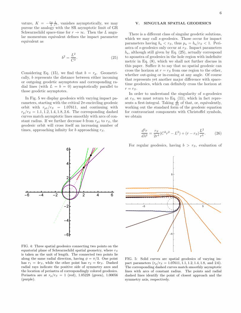
direction, having φ = π/3. One point has r1 = 4rS ,while the other point has r2 = 6rS . Periastra are atrp/rS = 1 (red), 1.05228 (green), 1.00056 (purple). Thered segment provides the shortest radial (L = 0) connec-tion between the two points. The green geodesic encirclesthe hole region once, crossing itself on the negative sideof the symmetry axis. The purple geodesic encircles thehole region twice and crosses itself twice, on both sidesof the symmetry axis.

FIG. 3: Four spatial geodesics connecting two points on theequatorial plane of Schwarzschild spatial geometry, where rSis taken as the unit of length. One point has r1 = 4rSand φ1 = π/4 + 1, while the other point has r2 = 5rS andφ2 = π/3 + 1. Dashed radial rays indicate the positive sideof symmetry axes and the location of periastra of correspond-ingly colored geodesics. Periastra are at rp/rS = 3.1838 (red),1.06209 (green), 1.04152 (purple), 1.00065 (blue).

To make further progress, we need to reframe thespatial geodetic analysis in terms of impact parame-ters. Given the fact that the intrinsic Gaussian cur-

6

vature, K = − rS2

1r3 , vanishes asymptotically, we may

pursue the analogy with the SR asymptotic limit of GRSchwarzschild space-time for r → ∞. Then the L angu-lar momentum equivalent defines the impact parameterequivalent as

b2 =L2

C2. (25)

Considering Eq. (15), we find that b = rp. Geometri-cally, b represents the distance between either incomingor outgoing geodetic asymptotes and corresponding ra-dial lines (with L = b = 0) asymptotically parallel tothose geodetic asymptotes.

In Fig. 5 we display geodesics with varying impact pa-rameters, starting with the critical 2π-encircling geodesicorbit with rp1/rS = 1.07611, and continuing withrp/rS = 1.1, 1.2, 1.4, 1.8, 2.6. The corresponding dashedcurves match asymptotic lines smoothly with arcs of con-stant radius. If we further decrease b from rp1 to rS , thegeodesic orbit will cross itself an increasing number oftimes, approaching infinity for b approaching rS .

FIG. 4: Three spatial geodesics connecting two points on theequatorial plane of Schwarzschild spatial geometry, where rSis taken as the unit of length. The connected two points liealong the same radial direction, having φ = π/3. One pointhas r1 = 4rS, while the other point has r2 = 6rS. Dashedradial rays indicate the positive side of symmetry axes andthe location of periastra of correspondingly colored geodesics.Periastra are at rp/rS = 1 (red), 1.05228 (green), 1.00056(purple).

V. SINGULAR SPATIAL GEODESICS

There is a different class of singular geodetic solutions,which we may call s-geodesics. Those occur for impactparameters having ba < rS , thus pa = ba/rS < 1. Peri-astra of s-geodesics only occur at rS . Impact parametersba, although still given by Eq. (25), actually correspondto apoastra of geodesics in the hole region with indefinitemetric in Eq. (8), which we shall not further discuss inthis paper. Suffice it to say that no spatial geodesic cancross the horizon at r = rS from one region to the other,whether out-going or in-coming at any angle. Of coursethat represents yet another major difference with space-time geodesics, which can definitely cross the horizon atr = rS .

In order to understand the singularity of s-geodesicsat rS , we must return to Eq. (11), which in fact repre-sents a first-integral. Taking d

dλ of that, or, equivalently,working out the standard form of the geodesic equationfor contravariant components with Christoffel symbols,we obtain

d2r

dλ2=

rS2r4

(C2r2 − L2) + (r − rS)L2

r4. (26)

For regular geodesics, having b > rS , evaluation of

-5 5

-5

5

FIG. 5: Solid curves are spatial geodesics of varying im-pact parameters (rp/rS = 1.07611, 1.1, 1.2, 1.4, 1.8, and 2.6).The corresponding dashed curves match smoothly asymptoticlines with arcs of constant radius. The points and radialdashed lines identify the point of closest approach and thesymmetry axis, respectively.

7

Eq. (26) at their rp periastron yields

(

d2r

dλ2

)

rp

= (rp − rS)L2

r4p> 0. (27)

However, for s-geodesics having ba < rS , evaluation ofEq. (26) at their rS periastron yields

(

d2r

dλ2

)

rS

=L2

2rS

(

1

b2a− 1

r2S

)

> 0. (28)

Clearly, the ‘acceleration equivalent’ in Eq. (27) hasa single value, whereas Eq. (28) involves a continuousrange of possibilities, having 0 < ba < rS . Thus, startingat any point with r ≥ rp > rS with any initial vector,there is a unique regular geodesic that transports thatvector parallel to itself indefinitely. However, startingat any point on the horizon, where grr diverges, thereis an infinite number of s-geodesics, all tangent to eachother and to the r = rS circle, that transport the sameinitial tangent vector parallel to itself and yet in all sub-sequently different directions. This situation is depictedin Fig. 6.

FIG. 6: Infinite number of s-geodesics, all tangent to eachother and to the r = rS = 1 circle at φ = 0, transportingthe same initial tangent vector parallel to itself and yet in allsubsequently different directions.

The situation is regularized on Flamm’s paraboloid, ifwe consider both surfaces with positive and negative Z-values, joined at the Z = 0 circle. In that perspective,the (Z, φ) coordinates produce a line element

dS2 =

(

1 +Z2

4r2S

)

(dZ)2 + r2S

(

1 +Z2

4r2S

)2

(dφ)2. (29)

That element is equal in value to dS2 in Eq. (13) for the(r, φ) coordinates, but the Z = 0 circle is no longer rep-resented as a line of coordinate singularities in Eq. (29).Thus, in Eq. (16) with ba replacing rp, the Z-elevation

of s-geodesics produces a unique tangent vector that in-tersects the Z = 0 circle at a specific angle γ such that

tan(γ) =

∣

∣

∣

∣

(

dZ

rdφ

)

rS

∣

∣

∣

∣

=

√

r2Sb2a

− 1. (30)

Examples of that are shown in Fig. 7.

FIG. 7: Solid curves are s-geodesics of varying pa (0.1, 0.3,0.5, 0.7, 0.9, and 0.99). The dashed circle indicates a radiusof rS = 1. Notice that only the innermost purple s-geodesicwith the greater pa = 0.99 fully encircles the hole region once.

Regularization of s-geodesics on the full Flamm’sparaboloid can also be appreciated by considering therelation

(

dZ

dλ

)2

=rSrgrr

(

dr

dλ

)2

. (31)

That produces a well defined limit

(

dZ

dλ

)2

rS

=L2

b2a− L2

r2S> 0 (32)

for r → rS , yielding Eq. (30), even though

(

dr

dλ

)2

rS

= 0. (33)

8

In terms of (r, φ) coordinates, s-geodesic solutions areobtained from Eq. (18) by setting its lower limit at r1 = 1

and by replacing p > 1 with pa < 1. Thus we obtain

φs(r) =

∫ r

1

pa dr√

r(r − 1)(r − pa)(r + pa)

= 2

√

pa1− pa

(

K

[

−1 + pa1− pa

]

+ iF

[

i sinh−1

(√

(1 − pa)(pa + r)

2pa(r − 1)

)

∣

∣

∣

∣

2

1− pa

])

. (34)

In the limit of r → ∞, the final angle is given by

φs,∞ = limr→∞

φs(r) = 2

√

pa1− pa

(

K

[

−1 + pa1− pa

]

+ iF

[

i sinh−1

(√

1− pa2pa

) ∣

∣

∣

∣

2

1− pa

])

. (35)

We may also invert Eq. (34) to obtain an explicit expres-sion of rs as a function of φ,

rs(φ) =

pa

(

1− sn[

i√

1−pa

4pa, 21−pa

]2)

sn[

i√

1−pa

4pa, 21−pa

]2

+ pa

, (36)

where sn denotes the Jacobi elliptic sine function, andthe angle φ is taken within the range (−φs,∞, φs,∞).Examples of s-geodesics of varying impact parameters,

with pa = ba/rS ≤ 1, are shown in Fig. 8. Notice againthat all s-geodesics obey Eq. (33), i.e., the rS-tangentialcondition. Continuation of s-geodesics at the horizon isnot shown in Fig. 6 or Fig. 8, while it is shown throughthe full Flamm’s paraboloid in Fig. 7.Having shown that s-geodesics parallel-transport their

tangent vectors continuously above and below the Z = 0circle on the full Flamm’s paraboloid, it is best to isomet-rically view the Schwarzschild geodesic equatorial planeas having two sides, joined at the horizon. Therein, s-geodesics parallel-transport their tangent vectors contin-uously through the r = rS horizon from the upper to thelower side, or conversely.For ba = 0 there are only radial geodesics, derived

from Eq. (11) for L = 0. That corresponds to continuousparabolae spanning both positive and negative Z-valueson the full Flamm’s paraboloid. Those parabolae inter-sect vertically the Z = 0 circle, with an angle γ = π/2,according to Eq. (30).For the critically separating value of b = ba = rS , the

point-particle spirals around the rS circle infinitely manytimes, without ever reaching it exactly. If it did, thegeodesic would transform into that of the r = rS circle.

The angle γ in Eq. (30) vanishes in that limit. It is stillpossible to solve analytically Eq. (18) for p = pa = 1,obtaining

-3 -2 -1 1

-2

-1

1

2

FIG. 8: Solid curves are s-geodesics of varying impact pa-rameters (pa = 0.1, 0.3, 0.5, 0.7, and 0.9). The correspondingdashed lines represent their asymptotes, parallel to the nega-tive X-axis. The dashed black line corresponds to the pa = 1limiting case.

9

φc(r) =

∫ ∞

r

dz

(z − 1)√

z(z + 1)=

1√2ln

(

3− 2√2)

(√r + 1

)(√r +

√2√r + 1 + 1

)

(√r − 1

)(

−√r +

√2√r + 1 + 1

)

. (37)

This solution is plotted as the dashed black curve inFig. 8, asymptotically starting parallel to the negativeX-axis with pa = 1 impact separation.

Let us now consider again any two points on the topside of the equatorial geodesic plane, say, or on the topsurface of Flamm’s paraboloid, equivalently. It is not al-ways possible to directly connect these two points withregular geodesics, as we did in Fig. 3 and Fig. 4, for exam-ple. When regular geodesics cannot directly connect thetwo points, s-geodesics can, and vice versa. There are dif-ferences, however. Only the shortest s-geodesic arc trulyconnects the two points on the same side of the equa-torial geodesic plane. Longer s-geodesic arcs that mayor may not encircle the hole region any number of timesare bound to fall into the other side of the equatorialgeodesic plane. From the perspective of the full Flamm’sparaboloid, longer s-geodesic arcs thus only connectpoints having opposite signs in their Z-coordinates. Ex-amples of this behavior are shown in Fig. 9 on the equa-torial geodesic plane, and more clearly in Fig. 10 on itsequivalent full Flamm’s paraboloid. Conversely, regulargeodesics are bound to one side of the equatorial geodesicplane. Thus, regular geodesics cannot connect pointshaving opposite signs in their Z-coordinates on the cor-responding full Flamm’s paraboloid.

Regular and s-geodesics together provide geodesiccompleteness, forming a one-parameter family of curveswith impact parameters ranging from −∞ to +∞. Fur-ther adding azimuthal symmetry, we may get a senseof the structure and space-filling distribution of regularand s-geodesics on the equatorial geodesic plane fromFig. 11 and Fig. 12, respectively. Equivalent renditionsof their embeddings on half and full Flamm’s paraboloidsare shown in Fig. 13 and Fig. 14, respectively.

It is of further interest to study independently geodesiccurvatures, κg, normal curvatures, κn, and relative tor-sions, τr, of curves embedded on Flamm’s paraboloid,using standard notions and elements of differentialgeometry.24,25 Geodesic curvatures must of course van-ish for all geodesics. Normal curvatures are illustratedon Flamm’s paraboloid in Fig. 15 for regular geodesicsand in Fig. 16 for s-geodesics, respectively. Plots of cor-responding normal curvatures are shown in Fig. 17. Lociof vanishing normal (thus total) curvatures reflect thevarying hyperbolic geometry of Flamm’s paraboloid. Wehave derived analytically and verified numerically manyother differential form and curvature results. Ultimately,however, all that analysis and results can be obtainedfrom the central geodesic orbit Eq. (16) and its exactsolutions that we have already provided. Therefore, we

shall not further report on such a complementary line ofinquiry within this context.

VI. GEODESIC ORBITS IN CURVED TIME

Let us alternatively consider a 4D pseudo-Riemannianmanifold with metric

ds2 =gµνdxµdxν

=−(

1− rSr

)

(cdt)2 + (dr)2+

r2(dθ)2 + r2 sin2 θ(dφ)2. (38)

-2 -1 1 2

-2

-1

1

2

FIG. 9: Three s-geodesics connecting two points of the equa-torial plane of Schwarzschild spatial geometry. One pointhas r1 = 1.5rS and φ1 = π/4, while the other point hasr2 = 1.25rS and φ2 = π/3. Dashed radial rays indicate thepositive side of symmetry axes and the location of perias-tra of correspondingly colored geodesics. All periastra occurat rS = 1. Impact parameters are ba/rS = 0.807342 (red),0.98445 (green), 0.999873 (purple). Only the red s-geodesicconnects two points on the same side of the Flamm embed-ding. The green and purple geodesics connect two points onopposite sides of the the Flamm embedding. Green and pur-ple s-geodesics fully encircle the hole region once and twice,respectively, while the red s-geodesic never does.

10

This differs from the physically correct Schwarzschildmetric in that the 3D spatial submanifold at any givencoordinate-time, t, is devoid of any curvature in Eq. (38).

Following the same procedures that we adopted earlier

FIG. 10: Flamm embedding of s-geodesics connecting twopoints on either sides of the equatorial plane in Fig. 9.

FIG. 11: Four grids of regular geodesics spanning each side ofthe spatial equatorial plane. Periastra originating each gridare taken at rp/rS = 1.1, 1.4, 1.7, and 2.0.

produces now the time-like geodesic orbit equation

(

dr

dφ

)2

=r4

L2

{

c2E2

(

1− G

c22M

r

)−1

− c2 − L2

r2

}

. (39)

This agrees with the Schwarzschild result in the non-relativistic Newtonian limit, whereas geodesic orbit equa-

FIG. 12: Nine grids of s-geodesics spanning both sides of thespatial equatorial plane. All periastra occur at rS = 1, withimpact parameters ba/rS ranging from 0.1 to 0.9 in steps of0.1.

FIG. 13: Flamm embedding of four grids of regular geodesics,spanning each side of the spatial equatorial plane in Fig. 11.

11

tions for the previous ‘splittable space-time’ metric,Eq. (17), do not.16 Historically, that was instrumentalfor Einstein to realize that Newtonian gravity basicallyderives from the equivalence principle and its association

FIG. 14: Flamm embedding of three grids of s-geodesics,spanning both sides of the spatial equatorial plane in Fig. 12.All periastra occur at rS = 1. Impact parameters are ba/rS =0.1, 0.5, and 0.9.

FIG. 15: Arcs of regular geodesics with positive (negative)normal curvatures are shown in green (red) on Flamm’sparaboloid.

with the gravitational redshift, even without full knowl-edge of Einstein field equations: cf. Chap. 18 of Ref. 5,for example.However, the null geodesic orbit equation for the grav-

itational red-shift or ‘curved-time’ metric of Eq. (38) is

(

dr

dφ

)2

=r4

L2

{

E2

c2

(

1− G

c22M

r

)−1

− L2

r2

}

, (40)

which differs profoundly from the exact null geodesic or-bit Eq. (7) of Schwarzschild space-time metric.Remarkably, however, turning points or apsides for

both time-like and null geodesics coincide for both ex-act and ‘curved-time’ metrics, Eq. (1) and Eq. (38). Inparticular, apsides of null geodesics for both metrics sat-isfy the same cubic equation

αp3 = p− 1, (41)

where

α =r2SE

2

c2L2. (42)

The three algebraic solutions to the cubic Eq. (41) addup to zero, according to Vieta’s formula, and are explic-

FIG. 16: Arcs of s-geodesics with positive (negative) normalcurvatures are shown in green (red) on Flamm’s paraboloid.The (normal) curvature of radial (L = 0) geodesics, κn =

κ = −1

2

√

rSr3

, is always negative, pointing away from the hole

region, although vanishing asymptotically.

12

itly

p1 =3√2(√

81α− 12− 9√α)2/3

+ 2 3√3

62/3 3

√√3√

α3(27α− 4)− 9α2

,

p2 =

3√−1(

3√−2(√

81α− 12− 9√α)2/3 − 2 3

√3)

62/3√α 3

√√81α− 12− 9

√α

,

p3 =2(−1)2/3 3

√3− 3

√−2(√

81α− 12− 9√α)2/3

62/3 3

√√3√

α3(27α− 4)− 9α2

. (43)

Depending on the value of α, we may have one, two,or no real and positive turning points. In fact, p2 isalways a real and negative solution, which must be phys-ically excluded. On the other hand, p1 and p3 are realand positive solutions for α < 4/27, representing twoturning points. For α > 4/27, p1 and p3 become com-plex conjugate solutions, implying no turning point. Forα = 4/27 = 0.148, these two real solutions merge into asingle turning point with p = 3/2, corresponding to anunstable circular orbit. That is well-known for photonsin Schwarzschild space-time, e.g., Eq. (11.18) in Ref. 4.The behavior of the solutions to the cubic Eq. (41) is

graphed in Fig. 18 as a function of α. That behavioris quite consistent with the effective potential for null

geodesics in Schwarzschild space-time, as shown in Fig.

1.00011.001

1.011.3

2.5

-5 0 5

0.0

0.2

0.4

0.6

0.8

1.0

Norm

alC

urvature(inr S)

0.2

0.40.6

0.8 0.9

0.99

0.999

0.9999

-5 0 5

-0.5

0.0

0.5

1.0

Angle ϕ from X axis (radians)

Norm

alC

urvature(inr S)

a)

b)

FIG. 17: Plots of normal curvature κn (in units of 1/rS = 1)vs. azimuthal angle φ (in radians) from the symmetry X-axis for: (a) five regular geodesics labeled by their periastrarp/rS > 1 within rectangular boxes; (b) eight s-geodesicslabeled by their impact parameters ba/rS < 1 within rectan-gular boxes.

11.2 of Ref. 4, for example. For the ‘curved-time’ met-ric, Eq. (38), the corresponding effective potential fornull geodesics becomes energy-dependent and divergingat rS . However, its basic features do not qualitativelydiffer from those pertaining to Schwarzschild space-timewith regard to the results that we have just provided forturning points of null geodesics.

FIG. 18: Solutions of the cubic Eq. (41). The parameter αis defined in Eq. (42). For α > 4/27 there are no positivereal solutions. The point p = 3/2 at which p1 and p3 coalesceintersects the vertical gray line where α = 4/27. Physically,that corresponds to an unstable circular orbit. For decreasingα, down to α → 0, p3 monotonically decreases toward rS = 1,marked by a horizontal gray line.

By the same method and procedures that we have ap-plied to study geodesics in Schwarzschild spatial submet-ric, Eq. (8), or ‘splittable space-time’ metric, Eq. (17),equivalently, we have obtained analytic solutions andnumerical results for all kinds of geodesics in both the‘curved-time’ metric, Eq. (38), and in Schwarzschild’sspace-time metric, Eq. (1). The latter study is criti-cally important, but too extensive to be reported here.26

Therefore, in the remainder of this Section, we will justconfine our discussion to comparisons of null-geodesic

asymptotic deflections for all three metrics considered.

For the parameters and limit of light grazing the sun,where rp = 235, 438rS, our results indicate a ‘spatialbending’ of half the total GR inward light deflectionof 1.75 arc-seconds, which we recover for the exact nullgeodesic orbit Eq. (7) of Schwarzschild space-time. Ourresults for the null geodesic Eq. (40) for the ‘curved-time’metric of Eq. (38) also indicate a ‘time bending’ of halfthe total GR deflection of 1.75 arc-seconds. Coinciden-tally, half of the correct GR deflection also agrees withthe much older prediction made by Cavendish (1784) andSoldner (1801) based on a purely Newtonian descriptionof light particles: cf. Ref. 8, Sec. 5.4, pp. 85-88, andRef. 27.

However, for a much closer approach of rp to rS , ‘timebending’ largely exceeds ‘spatial bending’ of light, whiletheir sum remains substantially below the total GR in-ward light deflection in Schwarzschild space-time. Somesignificant values are reported in Table 1. Asymptoticangular deflections vs. the periastron for null geodesicsfor all three metrics considered are plotted in Fig. 19.

13

rp/rS Curved Space Curved Time Sum GR Space-Time

1.5 68.61◦ – – –1.51 67.72◦ 298.9◦ 366.6◦ 529.0◦

1.6 60.76◦ 152.1◦ 212.8◦ 274.4◦

2 42.05◦ 67.09◦ 109.1◦ 125.1◦

5 13.04◦ 14.65◦ 27.69◦ 28.66◦

10 6.093◦ 6.423◦ 12.52◦ 12.71◦

100 34.58′ 34.75′ 1.156◦ 1.157◦

235,438 0.876′′ 0.876′′ 1.752′′ 1.752′′

TABLE I: Asymptotic angular deflections for some significantperiastron values of null geodesics in all three metrics consid-ered.

VII. CONCLUSIONS

We have solved geodesic orbit equations and character-ized corresponding manifolds for metrics associated withSchwarzschild geometry, considering space and time cur-vatures separately.For ‘fixed’ or ‘a-temporal’ space, with a positive-

definite submetric, Eq. (8), and for an essentially equiv-alent ‘splittable space-time’ metric, Eq. (17), we haveprovided a central geodesic orbit Eq. (16). We havesolved that equation in terms of elliptic integrals andfunctions. The intrinsic geometry of a geodesic equa-torial plane with two sides joined at the horizon corre-sponds to that of a full Flamm’s paraboloid. Two kinds

FIG. 19: Asymptotic angular deflections vs. periastron fornull geodesics in all three metrics considered. Black curve isfor ‘spatial bending’ with gtt = −1. Green curve is for ‘timebending’ with grr = 1. Blue curve is for Schwarzschild space-time metric with gtt ∗ grr = −1. The black-dashed curve rep-resents the sum of the black and green curves, i.e., the sum of‘spatial bending’ and ‘time bending.’ The two red-dashed ver-tical lines emphasize divergences at the Schwarzschild radius(rS = 1) for ‘spatial bending’ and at the radius of the unstablecircular orbit for either ‘curved-time’ or Schwarzschild space-time metrics (p = 3/2). Vertical and horizontal gray linesrefer to p = 5, 10 values and to corresponding Schwarzschildspace-time deflections, respectively.

of geodesics thus emerge. Both kinds may or may notencircle the hole region any number of times, crossingthemselves correspondingly. Regular geodesics reach aperiastron rp > rS , thus remaining confined to a half ofFlamm’s paraboloid. Singular or s-geodesics tangentiallyreach the rS circle. These s-geodesics must then be re-garded as funneling through the Z = 0 ‘belt’ of the fullFlamm’s paraboloid. Infinitely many geodesics can possi-bly be drawn between any two points, but they must be ofspecific regular or singular types. A precise classificationcan be made in terms of impact parameters. Geodesicstructure and completeness is conveyed by computer-generated figures depicting either Schwarzschild equato-rial plane or Flamm’s paraboloid.

For the ‘curved-time’ metric of Eq. (38), devoid of anyspatial curvature, geodesic orbits have the same apsidesas in Schwarzschild space-time. In particular, apsidesof null geodesics obey a cubic Eq. (41) that we solve.For the parameters and limit of light grazing the sun,asymptotic ‘spatial bending’ and ‘time bending’ becomeessentially equal, adding up to the total inward light de-flection of 1.75 arc-seconds predicted by GR. However,for a much closer approach of rp to rS , ‘time bending’largely exceeds ‘spatial bending’ of light, while their sumremains substantially below that of Schwarzschild space-time. These results are exact and generalize or clarifyprevious statements on that matter.20,21

Acknowledgments

The authors of this paper are listed in alphabet-ical order. We acknowledge financial support fromNASA/ADAP grants NNH11ZDA001N & NNX13AI48Gand from the Vitreous State Laboratory at the CatholicUniversity of America. We dedicate our work to thememory of Maria Rita Soverchia Resca.

14

∗ Electronic address: eufrasio@uark.edu ;URL: https://directory.uark.edu/people/eufrasio

† Electronic address: nmech@vsl.cua.edu‡ Electronic address: resca@cua.edu;URL: https://physics.catholic.edu/ ; correspond-ing author.

1 Grøn, Ø., Celebrating the centenary of the Schwarzschildsolutions, Am. J. Phys. 84(7), 537-541, July 2016.

2 Weinberg, S., Gravitation and Cosmology: Principles andApplications of the General Theory of Relativity, Wiley,New York, 1972.

3 Misner, C. W., Thorne, K. S., Wheeler, J. A., Gravitation,Freeman, New York, 1973.

4 Schutz, B. F., A First Course in General Relativity, 2ndEd., Cambridge University Press, 2009.

5 Schutz, B. F., Gravity from the Ground Up, CambridgeUniversity Press, 2003.

6 Wald, R. M., General Relativity, University of ChicagoPress, 1984.

7 Rindler, W., Essential Relativity: Special, General, andCosmological, Revised 2nd Ed., Springer-Verlag, 1979.

8 Berry, M., Principles of Cosmology and Gravitation, Cam-bridge University Press, 1976.

9 Hobson, M. P., Efstathiou, G. P., Lasenby, A. N., Gen-eral Relativity: An Introduction for Physicists, CambridgeUniversity Press, 2006.

10 Hartle, J. B., Gravity: An Introduction to Einstein’s Gen-eral Relativity, Pearson, 2003.

11 Frolov, V. P., Zelnikov, A., Introduction to Black HolePhysics, Oxford University Press, 2011.

12 Narlikar, J. V., Lectures on General Relativity and Cos-mology, Macmillan, New York, 1979.

13 Price, R. H., General relativity primer, Am. J. Phys.50(4), 300-329, April 1982.

14 Morris, M. S., Thorne, K. S., Wormholes in spacetime andtheir use for interstellar travel: A tool for teaching generalrelativity, Am. J. Phys. 56(5), 395-412, May 1988.

15 Dadhich, N., Einstein is Newton with space curved, Cur-rent Science, 109(2), 260-264, 25 July 2015.

16 Lorenzo Resca, 2018, Eur. J. Phys. 39, 035602 (14pp),Spacetime and spatial geodesic orbits in Schwarzschild ge-ometry, https://doi.org/10.1088/1361-6404/aab12f .

17 O’Neill, B., Semi-Riemannian Geometry with Applicationsto Relativity, Academic Press, New York, 1983.

18 Flamm, L., Beitrage zur Einsteinischen gravitationthe-ory, Physikalische Zeitschrift 17, 448-454, 1916. Trans-lation and Republication of: Contributions to Einstein’stheory of gravitation, by Ludwig Flamm, 30 May 2015,https://doi.org/10.1007/s10714-015-1908-2.

19 Einstein, A., Rosen, N., The particle problem in the gen-eral theory of relativity, Phys. Rev. 48, 73-77, 1935.

20 Price, R. H., Spatial curvature, spacetime curvature, andgravity, Am. J. Phys. 84(8), 588-592, August 2016.

21 Ellingson, J. G., The deflection of light by the Sun dueto three-space curvature, Am. J. Phys. 55(8), 759-760,August 1987.

22 Gruber, R. P., Gruber, A. D., Hamilton, R., Matthews,S. M., Space curvature and the ‘heavy banana paradox’,Phys. Teach. 29, 147-149, March 1991.

23 Olver, F. W. J., Olde Daalhuis, A. B., Lozier, D. W.,Schneider, B. I., Boisvert, R. F., Clark, C. W., Miller,B. R., Saunders, B. V, Editors, NIST Digital Libraryof Mathematical Functions, Release 1.0.18 of 2018-03-27,https://dlmf.nist.gov/.

24 do Carmo, M. P., Differential Geometry of Curves and Sur-faces : Revised and Updated 2nd Ed., Dover Publications,New York, 2017.

25 Pressley, A., Elementary Differential Geometry, 2nd Ed.,Springer-Verlag, London, New York, 2012.

26 Mecholsky, N. A., unpublished, 2018.27 Will, C. M., Henry Cavendish, Johann von Soldner, and

the deflection of light, Am. J. Phys. 56(5), 413-415, May1988.