Geometry and integrability of quadratic systems with ...
56
Electronic Journal of Qualitative Theory of Differential Equations 2021, No. 6, 1–56; https://doi.org/10.14232/ejqtde.2021.1.6 www.math.u-szeged.hu/ejqtde/ Geometry and integrability of quadratic systems with invariant hyperbolas Regilene Oliveira B 1 , Dana Schlomiuk 2 and Ana Maria Travaglini 1 1 Departamento de Matemática, ICMC-Universidade de São Paulo, Avenida Trabalhador São-carlense, 400 - 13566-590, São Carlos, SP, Brazil 2 Département de Mathématiques et de Statistique, Université de Montréal, CP 6128 succ. Centre-Ville, Montréal QC H3C 3J7, Canada Received 15 July 2020, appeared 18 January 2021 Communicated by Gabriele Villari Abstract. Let QSH be the family of non-degenerate planar quadratic differential sys- tems possessing an invariant hyperbola. We study this class from the viewpoint of integrability. This is a rich family with a variety of integrable systems with either poly- nomial, rational, Darboux or more general Liouvillian first integrals as well as non- integrable systems. We are interested in studying the integrable systems in this family from the topological, dynamical and algebraic geometric viewpoints. In this work we perform this study for three of the normal forms of QSH, construct their topological bifurcation diagrams as well as the bifurcation diagrams of their configurations of in- variant hyperbolas and lines and point out the relationship between them. We show that all systems in one of the three families have a rational first integral. For another one of the three families, we give a global answer to the problem of Poincaré by produc- ing a geometric necessary and sufficient condition for a system in this family to have a rational first integral. Our analysis led us to raise some questions in the last section, relating the geometry of the invariant algebraic curves (lines and hyperbolas) in the systems and the expression of the corresponding integrating factors. Keywords: quadratic differential systems, invariant algebraic curves, invariant hyper- bola, Darboux integrability, Liouvillian integrability. 2020 Mathematics Subject Classification: 34A05, 34C05, 34C45. 1 Introduction Let R[ x, y] be the set of all real polynomials in the variables x and y. Consider the planar system ˙ x = P( x, y), ˙ y = Q( x, y), (1.1) B Corresponding author. Email: [email protected]
Transcript of Geometry and integrability of quadratic systems with ...
Electronic Journal of Qualitative Theory of Differential Equations2021, No. 6, 1–56; https://doi.org/10.14232/ejqtde.2021.1.6 www.math.u-szeged.hu/ejqtde/
Geometry and integrability of quadratic systemswith invariant hyperbolas
Regilene OliveiraB 1, Dana Schlomiuk2 and Ana Maria Travaglini1
1Departamento de Matemática, ICMC-Universidade de São Paulo, Avenida Trabalhador São-carlense,400 - 13566-590, São Carlos, SP, Brazil
2Département de Mathématiques et de Statistique, Université de Montréal, CP 6128 succ. Centre-Ville,Montréal QC H3C 3J7, Canada
Received 15 July 2020, appeared 18 January 2021
Communicated by Gabriele Villari
Abstract. Let QSH be the family of non-degenerate planar quadratic differential sys-tems possessing an invariant hyperbola. We study this class from the viewpoint ofintegrability. This is a rich family with a variety of integrable systems with either poly-nomial, rational, Darboux or more general Liouvillian first integrals as well as non-integrable systems. We are interested in studying the integrable systems in this familyfrom the topological, dynamical and algebraic geometric viewpoints. In this work weperform this study for three of the normal forms of QSH, construct their topologicalbifurcation diagrams as well as the bifurcation diagrams of their configurations of in-variant hyperbolas and lines and point out the relationship between them. We showthat all systems in one of the three families have a rational first integral. For anotherone of the three families, we give a global answer to the problem of Poincaré by produc-ing a geometric necessary and sufficient condition for a system in this family to havea rational first integral. Our analysis led us to raise some questions in the last section,relating the geometry of the invariant algebraic curves (lines and hyperbolas) in thesystems and the expression of the corresponding integrating factors.
Keywords: quadratic differential systems, invariant algebraic curves, invariant hyper-bola, Darboux integrability, Liouvillian integrability.
2020 Mathematics Subject Classification: 34A05, 34C05, 34C45.
1 Introduction
Let R[x, y] be the set of all real polynomials in the variables x and y. Consider the planarsystem
x = P(x, y),
y = Q(x, y),(1.1)
BCorresponding author. Email: [email protected]

2 R. Oliveira, D. Schlomiuk and A. M. Travaglini
where x = dx/dt, y = dy/dt and P, Q ∈ R[x, y]. We call the degree of system (1.1) the integermaxdeg P, deg Q. In the case when the polynomial P and Q are relatively prime i. e. theydo not have a non-constant common factor, we say that (1.1) is non-degenerate.
Considerχ = P(x, y)
∂
∂x+ Q(x, y)
∂
∂y(1.2)
the polynomial vector field associated to (1.1).
A real quadratic differential system is a polynomial differential system of degree 2, i.e.
x = p0 + p1(a, x, y) + p2(a, x, y) ≡ p(a, x, y),
y = q0 + q1(a, x, y) + q2(a, x, y) ≡ q(a, x, y)(1.3)
wherep0 = a, p1(a, x, y) = cx + dy, p2(a, x, y) = gx2 + 2hxy + ky2,
q0 = b, q1(a, x, y) = ex + f y, q2(a, x, y) = lx2 + 2mxy + ny2.
Here we denote by a = (a, c, d, g, h, k, b, e, f , l, m, n) the 12-tuple of the coefficients of system(1.3). Thus a quadratic system can be identified with a point a in R12.
We denote the class of all real quadratic differential systems with QS.
In this work we are interested in polynomial differential equations (1.1) which are endowedwith an algebraic geometric structure, i.e. which posses invariant algebraic curves under theflow. We are interested both in their geometry and also in the impact this geometry has onthe integrability of the systems.
Definition 1.1 ([11]). An algebraic curve C(x, y) = 0 with C(x, y) ∈ C[x, y] is called an invariantalgebraic curve of system (1.1) if it satisfies the following identity:
CxP + CyQ = KC, (1.4)
for some K ∈ C[x, y] where Cx and Cy are the derivative of C with respect to x and y. K iscalled the cofactor of the curve C = 0.
For simplicity we write the curve C instead of the curve C = 0 in C2. Note that if system(1.1) has degree m then the cofactor of an invariant algebraic curve C of the system has degreem− 1.
Definition 1.2. Let U be an open subset of R2. A real function H: U → R is a first inte-gral of system (1.1) if it is constant on all solution curves (x(t), y(t)) of system (1.1), i.e.,H(x(t), y(t)) = k, where k is a real constant, for all values of t for which the solution(x(t), y(t)) is defined on U.
If H is differentiable in U then H is a first integral on U if and only if
HxP + HyQ = 0. (1.5)
Definition 1.3. If a system (1.1) has a first integral of the form
H(x, y) = C1λ1 · · ·Cp
λp (1.6)
where Ci are invariant algebraic curves of system (1.1) and λi ∈ C then we say that system(1.1) is Darboux integrable and we call the function H a Darboux function.

Geometry and integrability of QS with invariant hyperbolas 3
Theorem 1.4 ([11]). Suppose that a polynomial system (1.1) has m invariant algebraic curvesCi(x, y) = 0, i ≤ m, with Ci ∈ C[x, y] and with m > n(n + 1)/2 where n is the degree of thesystem. Then there exist complex numbers λ1, . . . , λm such that Cλ1
1 . . . Cλmm is a first integral of the
system.
If a system (1.1) admits a rational first integral we say that (1.1) is algebraically integrable.Poincaré was enthustiastic about the work of Darboux [11] which he called “oeuvre magis-trale” in [22] and stated the problem of algebraic integrability which asks to recognize when apolynomial vector field has a rational first integral. Jouanolou gave a sufficient condition forrecognizing that a polynomials system has a rational first integral.
Theorem 1.5 ([15]). Consider a polynomial system (1.1) of degree n and suppose that it admits minvariant algebraic curves Ci(x, y) = 0 where 1 ≤ i ≤ m, then if m ≥ 2+ n(n+1)
2 , there exists integersN1, N2, . . . , Nm such that I(x, y) = ∏m
i=1 CNii is a first integral of (1.1).
In connection to this problem Poincaré stated a number of definitions among them thefollowing definitions below.
Let H = f /g be a rational first integral of the polynomial vector field (1.2). We say thatH has degree n if n is the maximum of the degrees of f and g. We say that the degree of His minimal among all the degrees of the rational first integrals of χ if any other rational firstintegral of χ has a degree greater than or equal to n. Let H = f /g be a rational first integralof χ. According to Poincaré [22] we say that c ∈ C ∪ ∞ is a remarkable value of H if f + cgis a reducible polynomial in C[x, y]. Here, if c = ∞, then f + cg denotes g. Note that for allc ∈ C the algebraic curve f + cg = 0 is invariant. The curves in the factorization of f + cg,when c is a remarkable value, are called remarkable curves.
Now suppose that c is a remarkable value of a rational first integral H and that uα11 · · · uα
ris the factorization of the polynomial f + cg into reducible factors in C[x, y]. If at least one ofthe αi is larger than 1 then we say, following again Poincaré (see for instance [14]), that c is acritical remarkable value of H, and that ui = 0 having αi > 1 is a critical remarkable curve of thevector field (1.2) with exponent αi.
Since we can think of c ∈ C∪∞ as the projective line P1(R) we can also use the followingdefinition.
Definition 1.6. Consider F(c1,c2) : c1 f − c2g = 0 where f /g is a rational first integral of (1.2).We say that [c1 : c2] is a remarkable value of the curve F(c1,c2) if F(c1,c2) is reducible over C.
It is proved in [4] that there are finitely many remarkable values for a given rational firstintegral H and if (1.2) has a rational first integral and has no polynomial first integrals, thenit has a polynomial inverse integrating factor if and only if the first integral has at most twocritical remarkable values.
Given H = f /g a rational first integral, consider F(c1,c2) = c1 f − c2g where deg F(c1,c2) = n.If F(c1,c2) = f1 f2 where deg fi = ni < n then necessarily the points on the intersection of f1 = 0and f2 = 0 must be singular points of the curve F(c1,c2). So to find the irreducible factorsof F(c1,c2) we start by finding the singularities of F(c1,c2), i.e., the points on the curve whichannihilate both first derivatives in x and y.
The following notion was defined by Christopher in [5] where he called it “degenerateinvariant algebraic curve”.

4 R. Oliveira, D. Schlomiuk and A. M. Travaglini
Definition 1.7. Let F(x, y) = exp( G(x,y)
H(x,y)
)with G, H ∈ C[x, y] coprime. We say that F is an
exponential factor of system (1.1) if it satisfies the equality
FxP + FyQ = LF, (1.7)
for some L ∈ C[x, y]. The polynomial L is called the cofactor of the exponential factor F.
Definition 1.8. If system (1.1) has a first integral of the form
H(x, y) = C1λ1 · · ·Cp
λp F1µ1 · · · Fq
µq (1.8)
where Ci and Fj are the invariant algebraic curves and exponential factors of system (1.1)respectively and λi, µj ∈ C, then we say that the system is generalized Darboux integrable. Wecall the function H a generalized Darboux function.
Remark 1.9. In [11] Darboux considered functions of the type (1.6), not of type (1.8). In recentworks functions of type (1.8) were called Darboux functions. Since in this work we need to payattention to the distinctions among the various kinds of first integral we call (1.6) a Darbouxand (1.8) a generalized Darboux first integral.
Definition 1.10. Let U be an open subset of R2 and let R : U → R be an analytic functionwhich is not identically zero on U. The function R is an integrating factor of a polynomialsystem (1.1) on U if one of the following two equivalent conditions holds:
div(RP, RQ) = 0, RxP + RyQ = −R div(P, Q), (1.9)
on U.
A first integral H ofx = RP, y = RQ
associated to the integrating factor R is given by
H(x, y) =∫
R(x, y)P(x, y)dy + h(x),
where H(x, y) is a function satisfying Hx = −RQ. Then,
x = Hy, y = −Hx.
In order that this function H be well defined the open set U must be simply connected.
Liouvillian functions are functions that are built up from rational functions using expo-nentiation, integration, and algebraic functions. For more details on Liouvillian functions,see [7].
Theorem 1.11 ([4, 21]). If a planar polynomial vector field (1.2) has a generalized Darboux firstintegral, then it has a rational integrating factor.
As for a converse, we have the following result which easily follows from [23].
Theorem 1.12 ([8]). If a planar polynomial vector field (1.2) has a rational integrating factor, then ithas a generalized Darboux first integral.
An important consequence of Singer’s theorem (see [27]) is the following.

Geometry and integrability of QS with invariant hyperbolas 5
Theorem 1.13 ([5, 27]). A planar polynomial differential system (1.1) has a Liouvillian first integralif and only if it has a generalized Darboux integrating factor.
For a proof see [28, p. 134].We have the following table summing up these results.
First integral Integrating factorGeneralized Darboux ⇔ Rational
Liouvillian ⇔ Generalized Darboux
Definition 1.14 ([11]). Consider a planar polynomial system (1.1). An algebraic solution f = 0of (1.1) is an algebraic invariant curve which is irreducible over C.
Theorem 1.15 ([6]). Consider a polynomial system (1.1) that has k algebraic solutions Ci = 0 suchthat
(a) all curves Ci = 0 are non-singular and have no repeated factor in their highest order terms,
(b) no more than two curves meet at any point in the finite plane and are not tangent at these points,
(c) no two curves have a common factor in their highest order terms,
(d) the sum of the degrees of the curves is n + 1, where n is the degree of system (1.1).
Then system (1.1) has an integrating factor
µ(x, y) = 1/(C1C2 · · ·Ck).
This result of Christopher–Kooij (C–K) is interesting because it relates the geometry of theconfiguration of invariant algebraic curves of the systems with the expression of the integrat-ing factors involving the polynomials defining the curves. In fact this theorem has a geometriccontent which is however not completely explicit in the algebraic way their theorem is stated.We restate the above result in geometric terms as follows:
Theorem 1.16. Consider a polynomial system (1.1) that has k algebraic solutions Ci = 0 such that
(a) all curves Ci = 0 are non-singular and they intersects transversally the line at infinity Z = 0,
(b) no more than two curves meet at any point in the finite plane and are not tangent at these points,
(c) no two curves intersect at a point on the line at infinity Z = 0,
(d) the sum of the degrees of the curves is n + 1, where n is the degree of system (1.1).
Then system (1.1) has an integrating factor
µ(x, y) = 1/(C1C2 · · ·Ck).
In the hypotheses of this theorem the way the curves are placed with respect to one anotherin the totality of the curves, in other words the “geometry of the configuration of invariantalgebraic curves” has an impact of the kind of integrating factor we could have. One of ourgoals is to collect data so as to extend this theorem beyond these limiting geometric conditions.

6 R. Oliveira, D. Schlomiuk and A. M. Travaglini
There are some important invariant polynomials in the study of polynomial vector fields.Considering C2(a, x, y) = yp2(a, x, y)− xq2(a, x, y) as a cubic binary form of x and y we calcu-late
η(a) = Discrim[C2, ξ], M(a, x, y) = Hessian[C2],
where ξ = y/x or ξ = x/y. It is known that the singular points at infinity of quadratic systemsare given by the solutions in x and y of C2(a, x, y) = 0. If η < 0 then this means we have onereal singular point at infinity and two complex.
Remark 1.17. We note that since a system in QSH always has an invariant hyperbola thenclearly we always have at least 2 real singular points at infinity. So we must have η ≥ 0.
The family QSH can be split as follows: QSH(η=0) of systems which possess either exactlytwo distinct real singularities at infinity or the line at infinity filled up with singularities andQSH(η>0) of systems which possess three distinct real singularities at infinity in P2(C).
In [18] the authors proved that there are 162 distinct configurations and provided necessaryand sufficient conditions for a non-degenerate quadratic differential system to have at leastone invariant hyperbola and for the realization of each one of the configurations. Theseconditions are expressed in terms of the coefficients of the systems. They obtained the normalforms for family QSH and in this paper we study the following 3 normal forms:
x = a− x2
3 −2xy
3
y = 4a− 3v2 − 4xy3
+y2
3, where a 6= 0.
(1.10)
x = − x2
2− xy
2
y = b− 3xy2
+y2
2, where b 6= 0.
(1.11)
x = 2a + gx2 + xy,
y = a(2g− 1) + (g− 1)xy + y2, where a(g− 1) 6= 0.(1.12)
Our first goal in this paper is to do a complete study of these three families of quadraticsystems which possess an invariant hyperbola. Our interest is in the geometry of these sys-tems, as expressed in terms of their invariant algebraic curves, in the impact of this geometryon the integrability of these systems, on their phase portraits and in the dynamics of thesystems expressed in the bifurcation diagrams of the families we study. Our third goal is toconfront our results with the existing results in the literature and bring to light some missingcases in theses other studies which we point out here. Our geometric analysis is done in detailas this is part of a program of collecting data in order to obtain more global results on thefamily QSH and its Darboux theory.
Our paper is organized as follows: in Section 2 we give a number of definitions andpropositions useful for the other sections. In Sections 3, 4, 5 we present a complete study offamilies (1.10), (1.11) and (1.12). The choice of the first two families is motivated by the factthat they do not satisfy all the conditions in the hypothesis of the Christopher–Kooij theorem,here stated in theorem 1.15, but the conclusion of the theorem still holds, while the last familydoes not always posses a first integral and it will provide a counterpoint. In Section 6 weraise some questions, consider the problem of Poincaré for the family QSH, and make someconcluding comments.

Geometry and integrability of QS with invariant hyperbolas 7
2 Preliminaries
The notion of configuration of invariant curves of a polynomial differential system appears inseveral works, see for instance [26].
Definition 2.1. Consider a real planar polynomial system (1.1) with a finite number of singularpoints. By a configuration of algebraic solutions of the system we mean a set of algebraic solutionsover C of the system, each one of these curves endowed with its own multiplicity and togetherwith all the real singular points of this system located on these curves, each one of thesesingularities endowed with its own multiplicity.
Definition 2.2. Suppose we have two systems (S1), (S2) in QSH with a finite number ofsingularities, finite or infinite, a finite set of invariant hyperbolas H1
i : h1i (x, y) = 0, i = 1, . . . , k
of (S1) (respectively H2i : h2
i (x, y) = 0, i = 1, . . . , k of (S2)) and a finite set (which couldalso be empty) of invariant straight lines L1
j : g1j (x, y) = 0, j = 1, . . . , k′ of (S1) (respectively
L2j : g2
j (x, y) = 0, j = 1, . . . , k′ of (S2)). We say that the two configurations C1, C2 of hyperbolasand lines of these systems are equivalent if there is a one-to-one correspondence Φh betweenthe hyperbolas of C1 and C2 and a one-to-one correspondence Φl between the lines of C1 andC2 such that:
(i) the correspondences conserve the multiplicities of the hyperbolas and lines (in case thereare any) and also send a real invariant curve to a real invariant curve and a complexinvariant curve to a complex invariant curve;
(ii) for each hyperbola H : h(x, y) = 0 of C1 (respectively each line L : g(x, y) = 0) we have aone-to-one correspondence between the real singular points onH (respectively on L) andthe real singular points on Φh(H) (respectively Φl(L)) conserving their multiplicities,their location on branches of hyperbolas and their order on these branches (respectivelyon the lines);
(iii) Furthermore, consider the total curves F 1 : ∏ H1i (X, Y, Z)∏ G1
j (X, Y, Z)Z = 0 (respec-tively F 2 : ∏ H2
i (X, Y, Z)∏ G2j (X, Y, Z)Z = 0) where H1
i (X, Y, Z) = 0, G1j (X, Y, Z) = 0
(respectively H2i (X, Y, Z) = 0, G2
j (X, Y, Z) = 0) are the projective completions of H1i , L1
j
(respectively H2i , L2
j ). Then, there is a one-to-one correspondence ψ between the sin-gularities of the curves F 1 and F 2 conserving their multiplicities as singular points ofthese (total) curves.
It is important to assume that systems (1.3) are non-degenerate because otherwise doing atime rescaling, they can be reduced to linear or constant systems. Under this assumption allthe systems in QSH have a finite number of finite singular points.
In the family QSH we also have cases where we have an infinite number of hyperbolas.In these cases, by a Jouanolou result (see Theorem 1.5 on page 3), we have a rational firstintegral.
In [18] the authors classified the family QSH, according to their geometric properties en-coded in the configurations of invariant hyperbolas and invariant straight lines which thesesystems possess. If a quadratic system has an infinite number of hyperbolas then the systemhas a finite number of invariant affine straight lines (see [1]). Therefore, we can talk aboutequivalence of configurations of the invariant affine lines associated to the system. Given two such

8 R. Oliveira, D. Schlomiuk and A. M. Travaglini
configurations C1l and C2l associated to systems (S1) and (S2) of (1.1), we say they are equiva-lent if and only if there is a one-to-one correspondence Φ between the lines of C1l and C2l suchthat:
(i) the correspondence preserve the multiplicities of the lines and also sends a real (respec-tively complex) invariant line to a real (respectively complex) invariant line;
(ii) for each line L : g(x, y) = 0 we have a one-to-one correspondence between the realsingularities on L and the real singularities on Φ preserving their multiplicities and theirorder on the lines.
Definition 2.3 ([18]). Consider two systems (S1) and (S2) in QSH each one with an infinitenumber of invariant hyperbolas. Consider the configurations C1l and C2l of invariant affinestraight lines L1
j : g1j (x, y) = 0 where j = 1, 2, . . . , k of system (S1) and respectively L2
j :g2
j (x, y) = 0 where j = 1, 2, . . . , k of system (S2). We say that the two configurations C1l andC2l are equivalent with respect to the hyperbolas of the systems if and only if:
(i) they are equivalent as configurations of invariant lines, and
(ii) taking any hyperbola H1 : h1(x, y) = 0 of (S1) and any hyperbola H2 : h2(x, y) = 0of (S2), then we must have a one-to-one correspondence between the real singularitiesof system (S1) located on H1 and of real singularities of system (S2) located on H2,preserving their multiplicities, their location and order on branches.
Furthermore, consider the curves F1 : ∏ h1(x, y)∏ g1j = 0 and F2 : ∏ h2(x, y)∏ g2
j = 0.Then, we have a one-to-one correspondence between the singularities of the curve F1 withthose in the curve F2 preserving their multiplicities as singularities of these curves.
The definition above is independent of the choice of the two hyperbolas H1 : h1(x, y) = 0of (S1) and H2 : h2(x, y) = 0 of (S2).
Suppose that a polynomial differential system has an algebraic solution f (x, y) = 0 wheref (x, y) ∈ C[x, y] is of degree n given by
f (x, y) = c0 + c10x + c01y + c20x2 + c11xy + c02y2 + · · ·+ cn0xn + cn−1,1xn−1y + · · ·+ c0nyn,
with c = (c0, c10, . . . , c0n) ∈ CN where N = (n + 1)(n + 2)/2. We note that the equation
λ f (x, y) = 0, λ ∈ C∗ = C− 0
yields the same locus of complex points in the plane as the locus induced by f (x, y) = 0.Therefore, a curve of degree n is defined by c where
[c] = [c0 : c10 : · · · : c0n] ∈ PN−1(C).
We say that a sequence of curves fi(x, y) = 0, each one of degree n, converges to a curvef (x, y) = 0 if and only if the sequence of points [ci] = [ci0 : ci10 : · · · : ci0n] converges to[c] = [c0 : c10 : · · · : c0n] in the topology of PN−1(C).
We observe that if we rescale the time t′ = λt by a positive constant λ the geometry of thesystems (1.1) (phase curves) does not change. So for our purposes we can identify a system(1.1) of degree n with a point
[a0 : a10 : · · · : a0n : b0 : b10 : · · · : b0n] ∈ SN−1(R)
where N = (n + 1)(n + 2).

Geometry and integrability of QS with invariant hyperbolas 9
Definition 2.4.
(1) We say that an invariant curve
L : f (x, y) = 0, f ∈ C[x, y]
for a polynomial system (S) of degree n has geometric multiplicity m if there exists asequence of real polynomial systems (Sk) of degree n converging to (S) in the topologyof SN−1(R) where N = (n+ 1)(n+ 2) such that each (Sk) has m distinct invariant curves
L1,k : f1,k(x, y) = 0, . . . ,Lm,k : fm,k(x, y) = 0
over C, deg( f ) = deg( fi,k) = r, converging to L as k → ∞, in the topology of PR−1(C),with R = (r + 1)(r + 2)/2 and this does not occur for m + 1.
(2) We say that the line at infinityL∞ : Z = 0
of a polynomial system (S) of degree n has geometric multiplicity m if there exists asequence of real polynomial systems (Sk) of degree n converging to (S) in the topologyof SN−1(R) where N = (n + 1)(n + 2) such that each (Sk) has m− 1 distinct invariantlines
L1,k : f1,k(x, y) = 0, . . . ,Lm−1,k : fm−1,k(x, y) = 0
over C, converging to the line at infinity L∞ as k→ ∞, in the topology of P2(C) and thisdoes not occur for m.
Definition 2.5 ([9]). Let Cm[x, y] be the C-vector space of polynomials in C[x, y] of degree atmost m and of dimension R = (2+m
2 ). Let v1, v2, . . . , vR be a base of Cm[x, y]. We denote byMR(m) the R× R matrix
MR(m) =
v1 v2 . . . vR
χ(v1) χ(v2) . . . χ(vR)...
.... . .
...χR−1(v1) χR−1(v2) . . . χR−1(vR)
, (2.1)
where χk+1(vi) = χ(χk(vi)). The mth extactic curve of χ, Em(χ), is given by the equationdet MR(m) = 0. We also call Em(χ) the mth extactic polynomial.
From the properties of the determinant we note that the extactic curve is independent ofthe choice of the base of Cm[x, y].
Theorem 2.6 ([20]). Consider a planar vector field (1.2). We have Em(χ) = 0 and Em−1(χ) 6= 0 ifand only if χ admits a rational first integral of exact degree m.
Observe that if f = 0 is an invariant algebraic curve of degree m of χ , then f dividesEm(χ). This is due to the fact that if f is a member of a base of Cm[x, y], then f divides thewhole column in which f is located.
Definition 2.7 ([9]). We say that an invariant algebraic curve f = 0 of degree m ≥ 1 hasalgebraic multiplicity k if det MR(m) 6= 0 and k is the maximum positive integer such that f k
divides det MR(m); and it has no defined algebraic multiplicity if det MR(m) ≡ 0.

10 R. Oliveira, D. Schlomiuk and A. M. Travaglini
Definition 2.8 ([9]). We say that an invariant algebraic curve f = 0 of degree m ≥ 1 hasintegrable multiplicity k with respect to χ if k is the largest integer for which the following istrue: there are k − 1 exponential factors exp(gj/ f j), j = 1, . . . , k − 1, with deg gj ≤ jm, suchthat each gj is not a multiple of f .
In the next result we see that the algebraic and integrable multiplicity coincide if f = 0 isan irreducible invariant algebraic curve.
Theorem 2.9 ([16]). Consider an irreducible invariant algebraic curve f = 0 of degree m ≥ 1 of χ.Then f has algebraic multiplicity k if and only if the vector field (1.2) has k − 1 exponential factorsexp(gj/ f j), where (gj, f ) = 1 and gj is a polynomial of degree at most jm, for j = 1, . . . , k− 1.
In [9] the authors showed that the definitions of geometric, algebraic and integrable mul-tiplicity are equivalent when f = 0 is an irreducible invariant algebraic curve of vector field(1.2).
In order to use the infinity of R2 as an additional invariant curve for studying the integra-bility of the vector field χ, we need the Poincaré compactification of the vector field χ. ForZ 6= 0 consider the change of variables
x =1Z
, y =YZ
the vector field χ is transformed to
χ = −Z P(Z, Y)∂
∂Z+(Q(Z, Y)−Y P(Z, Y)
) ∂
∂Y
where P(Z, Y) = Z2P( 1
Z , YZ
)and Q(Z, Y) = Z2Q
( 1Z , Y
Z
).
We note that Z = 0 is an invariant line of the vector field χ and that the infinity of R2
corresponds to Z = 0 of the vector field χ. So we can define the algebraic multiplicity ofZ = 0 for the vector field χ.
Definition 2.10. We say that the infinity of χ has algebraic multiplicity k if Z = 0 has algebraicmultiplicity k for the vector field χ; and that it has no defined algebraic multiplicity if Z = 0has no defined algebraic multiplicity for χ.
Let’s recall the algebraic-geometric definition of an r-cycle on an irreducible algebraicvariety of dimension n.
Definition 2.11. Let V be an irreducible algebraic variety of dimension n over a field K. Acycle of dimension r or r-cycle on V is a formal sum
∑W
nWW
where W is a subvariety of V of dimension r which is not contained in the singular locus ofV, nW ∈ Z, and only a finite number of nW ’s are non-zero. We call degree of an r-cycle thesum
∑W
nW .
An (n− 1)-cycle is called a divisor.

Geometry and integrability of QS with invariant hyperbolas 11
Definition 2.12. For a non-degenerate polynomial differential systems (S) possessing a finitenumber of algebraic solutions
F = fimi=1, fi(x, y) = 0, fi(x, y) ∈ C,
each with multiplicity ni and a finite number of singularities at infinity, we define the algebraicsolutions divisor (also called the invariant curves divisor) on the projective plane,
ICDF = ∑ni
niCi + n∞L∞
where Ci : Fi(X, Y, Z) = 0 are the projective completions of fi(x, y) = 0, ni is the multiplicityof the curve Ci = 0 and n∞ is the multiplicity of the line at infinity L∞ : Z = 0.
It is well known (see [1]) that the maximum number of invariant straight lines, includingthe line at infinity, for polynomial systems of degree n ≥ 2 is 3n.
Proposition 2.13 ([1]). Every quadratic differential system has at most six invariant straight lines,including the line at infinity.
In the case we consider here, we have a particular instance of the divisor ICD because theinvariant curves will be invariant hyperbolas and invariant lines of a quadratic differentialsystem, in case these are in finite number. In case we have an infinite number of hyperbolaswe can construct the divisor of the invariant straight lines which are always in finite number.
Another ingredient of the configuration of algebraic solutions are the real singularitiessituated on these curves. We also need to use here the notion of multiplicity divisor of realsingularities of a system, located on the algebraic solutions of the system.
Definition 2.14.
1. Suppose a real quadratic system (1.3) has a non-zero finite number of invariant hyper-bolas
Hi : hi(x, y) = 0, i = 1, 2, . . . , k
and a finite number of affine invariant lines
Lj : f j(x, y) = 0, j = 1, 2, . . . , l.
We denote the line at infinity L∞ : Z = 0. Let us assume that on the line at infinity wehave a finite number of singularities. The divisor of invariant hyperbolas and invariantlines on the complex projective plane of the system is the following
ICD = n1H1 + · · ·+ nkHk + m1L1 + · · ·+ mlLl + m∞L∞
where ni (respectively mj) is the multiplicity of the hyperbola Hi (respectively mj of theline Lj), and m∞ is the multiplicity of L∞. We also mark the complex (non-real) invarianthyperbolas (respectively lines) denoting them by HC
i (respectively LCi ). We define the
total multiplicity TM of the divisor as the sum ∑i ni + ∑j mj + m∞.
2. The zero-cycle on the real projective plane, of singularities of a quadratic system (1.3)located on the configuration of invariant lines and invariant hyperbolas, is given by
M0CS = r1P1 + · · ·+ rl Pl + v1P∞1 + · · ·+ vnP∞
n
12 R. Oliveira, D. Schlomiuk and A. M. Travaglini
where Pi (respectively P∞j ) are all the finite (respectively infinite) such singularities of
the system and ri (respectively vj) are their corresponding multiplicities. We mark thecomplex singular points denoting them by PC
i . We define the total multiplicity TM ofzero-cycles as the sum ∑i ri + ∑j vj.
In the family QSH we have configurations which have an infinite number of hyperbolas.These are of two kinds: those with a finite number of singular points at infinity, and thosewith the line at infinity filled up with singularities. To distinguish these two cases we define|Sing∞| to be the cardinality of the set of singular points at infinity of the systems. In the firstcase we have |Sing∞| = 2 or 3, and in the second case |Sing∞| is the continuum and we simplywrite |Sing∞| = ∞. Since in both cases the systems admit a finite number of affine invariantstraight lines we can use them to distinguish the configurations.
Definition 2.15.
(1) In case we have an infinite number of hyperbolas and just two or three singular pointsat infinity but we have a finite number of invariant straight lines we define
ILD = m1L1 + · · ·+ mlLl + m∞L∞.
(2) In case we have an infinite number of hyperbolas, the line at infinity is filled up withsingularities and we have a finite number of affine lines, we define
ILD = m1L1 + · · ·+ mlLl .
Suppose we have a finite number of invariant hyperbolas and invariant straight lines of asystem (S) and that they are given by equations
fi(x, y) = 0, i ∈ 1, 2, . . . , k, fi ∈ C[x, y].
Let us denote by Fi(X, Y, Z) = 0 the projection completion of the invariant curves fi = 0 inP2(C).
Definition 2.16. The total invariant curve of the system (S) in QSH, on P2(R), is the curve
T(S) = ∏i
Fi(X, Y, Z)Z = 0.
In case one of the curves is multiple then it will appear with its multiplicity.
For example, if a system (S) admits an invariant hyperbola h(x, y) with multiplicity twoand the line at infinity Z = 0 has multiplicity one, then the total invariant curve of thissystem is
T(S) = H(X, Y, Z)2Z = 0
where H(X, Y, Z) = 0 is the projection completion of h = 0. The degree of T(S) is 5.The singular points of the system (S) situated on T(S) are of two kinds: those which are
simple (or smooth) points of T(S) and those which are multiple points of T(S).
Remark 2.17. To each singular point of the system we have its associated multiplicity as asingular point of the system. In addition, when these singular points are situated on the totalcurve, we also have the multiplicity of these points as points on the total curve T(S). Through

Geometry and integrability of QS with invariant hyperbolas 13
a singular point of the systems there may pass several of the curves Fi = 0 and Z = 0. Also wemay have the case when this point is a singular point of one or even of several of the curvesin case we work with invariant curves with singularities. This leads to the multiplicity of thepoint as point of the curve T(S). The simple points of the curve T(S) are those of multiplicityone. They are also the smooth points of this curve.
Definition 2.18. The zero-cycle of the total curve T(S) of system (S) is given by
M0CT = r1P1 + · · ·+ rl Pl + v1P∞1 + · · ·+ vnP∞
n
where Pi (respectively P∞j ) are all the finite (respectively infinite) singularities situated on T(S)
and ri (respectively vj) are their corresponding multiplicities as points on the total curve T(S).We define the total multiplicity TM of zero-cycles of the total invariant curve as the sum∑i ri + ∑j vj.
Remark 2.19. If two curves intersects transversally, this point will be a simple point of inter-section. If they are tangent, we would have an intersection multiplicity higher than or equalto two.
Definition 2.20 ([24]). Two polynomial differential systems S1 and S2 are topologically equiv-alent if and only if there exists a homeomorphism of the plane carrying the oriented phasecurves of S1 to the oriented phase curves of S2 and preserving the orientation.
To cut the number of non equivalent phase portraits in half we use here another equiva-lence relation.
Definition 2.21. Two polynomial differential systems S1 and S2 are topologically equivalent ifand only if there exists a homeomorphism of the plane carrying the oriented phase curves ofS1 to the oriented phase curves of S2, preserving or reversing the orientation.
We use the notation for singularities as introduced in [2] and [3]. We say that a singularpoint is elemental if it possess two eigenvalues not zero; semi-elemental if it possess exactly oneeigenvalue equal to zero and nilpotent if it posses two eigenvalues zero. We call intricate asingular point with its Jacobian matrix identically zero.
We will place first the finite singular points which will be denoted with lower case lettersand secondly we will place the infinite singular points which will be denoted by capital letters,separating them by a semicolon ’;’.
In our study we will have real and complex finite singular points and from the topologicalviewpoint only the real ones are interesting. When we have a simple (respectively double)complex finite singular point we use the notation © (respectively ©(2)).
For the elemental singular points we use the notation ’s’, ’S’ for saddles, ’n’, ’N’ for nodes,’ f ’ for foci and ’c’ for centers.
Non-elemental singular points are multiple points. Here we introduce a special notationfor the infinity non-elemental singular point. We denote by (a
b) the maximum number a (re-spectively b) of finite (respectively infinite) singularities which can be obtained by perturbationof the multiple point. For example, when we have a non-elemental point at infinity obtainedby the coalescence from a node at infinite with a saddle at infinite we will denoted it by (0
2)SN.The semi-elemental singular points can either be nodes, saddles or saddle-nodes (finite
or infinite). If they are finite singular points we will denote them by ’n(2)’, ’s(2)’ and ’sn(2)’,

14 R. Oliveira, D. Schlomiuk and A. M. Travaglini
respectively and if they are infinite singular points by ’(ab)N’, ’(a
b)S’ and ’(ab)SN’, where (a
b) in-dicates their multiplicity. We note that semi-elemental nodes and saddles are respectivelytopologically equivalent with elemental nodes and saddles.
The nilpotent singular points can either be saddles, nodes, saddle-nodes, elliptic-saddles,cusps, foci or centers. The only finite nilpotent points for which we need to introduce notationare the elliptic-saddles and cusps which we denote respectively by ’es’ and ’cp’.
The intricate singular points are degenerate singular points. It is known that the neigh-bourhood of any singular point of a polynomial vector field (except for foci and centers) isformed by a finite number of sectors which could only be of three types: parabolic (p), hyper-bolic (h) and elliptic (e) (see [12]). In this work we have the following finite intricate singularpoints of multiplicity four described according their sectoral decomposition:
• hpphpp(4)
• phph(4)
• epep(4)
The degenerate systems are systems with a common factor in the polynomials definingthe system. We will denote this case with the symbol . The degeneracy can be producedby a common factor of degree one which defines a straight line or a common quadratic factorwhich defines a conic. In this paper we have just the first case happening. Following [2] weuse the symbol [|] for a real straight line.
Moreover, we also want to determine whether after removing the common factor of thepolynomials, singular points remain on the curve defined by this common factor. If somesingular points remain on this curve we will use the corresponding notation of their variouskinds. In this situation, the geometrical properties of the singularity that remain after theremoval of the degeneracy, may produce topologically different phenomena, even if they aretopologically equivalent singularities. So, we will need to keep the geometrical informationassociated to that singularity.
In this study we use the notation ([|]; nd) which denotes the presence of a real straightline filled up with singular points in the system such that the reduced system has a node nd
on this line where nd is a one-direction node, that is, a node with two identical eigenvalueswhose Jacobian matrix cannot be diagonal.
The existence of a common factor of the polynomials defining the differential system alsoaffects the infinite singular points.
We point out that the projective completion of a real affine line filled up with singularpoints has a point on the line at infinity which will then be also a non-isolated singularity.There is a detailed description of this notation in [2]. In case that after the removal of the finitedegeneracy, a singular point at infinity remains at the same place, we must denote it with allits geometrical properties since they may influence the local topological phase portrait. In thisstudy we use the notation (0
2)SN, ([|]; ∅) that means that the system has at infinity a saddle-node, and one non-isolated singular point which is part of a real straight line filled up withsingularities (other that the line at infinity), and that the reduced linear system has no infinitesingular point in that position. See [2] and [3] for more details.
In order to distinguish topologically the phase portraits of the systems we obtained, wealso use some invariants introduced in [25]. Let SC be the total number of separatrix connec-tions, i.e. of phase curves connecting two singularities which are local separatrices of the twosingular points. We denote by

Geometry and integrability of QS with invariant hyperbolas 15
• SC ff the total number of SC connecting two finite singularities,
• SC∞f the total number of SC connecting a finite with an infinite singularity,
• SC∞∞ the total number of SC connecting two infinite.
A graphic as defined in [13] is formed by a finite sequence of singular points r1, r2, . . . , rn
(with possible repetitions) and non-trivial connecting orbits γi for i = 1, . . . , n such that γi hasri as α-limit set and ri+1 as ω-limit set for i < n and γn has rn as α-limit set and r1 as ω-limitset. Also normal orientations nj of the non-trivial orbits must be coherent in the sense that ifγj−1 has left-hand orientation then so does γj. A polycycle is a graphic which has a Poincaréreturn map.
A degenerate graphic is a graphic where it is also allowed that one or several (even all)connecting orbits γi can be formed by an infinite number of singular points. For more details,see [13].
3 Geometric analysis of family (1.10)
Consider the family
(1.10)
x = a− x2
3− 2xy
3
y = 4a− 3v2 − 4xy3
+y2
3, where a 6= 0.
This is a two parameter family depending on (a, v) ∈ (R\0) × R. We display belowthe full geometric analysis of the systems in this family, which is endowed with at least threeinvariant algebraic curves. In the generic situation
av(a− v2)(a− 3v2/4)(a + 3v2)(a− 8v2/9) 6= 0 (3.1)
the systems have only two invariant lines J1 and J2 and only two invariant hyperbolas J3 andJ4 with respective cofactors αi, 1 ≤ i ≤ 4 where
J1 = −3√−a + v2 − x + y, α1 =
√−a + v2 − x
3 + y3 ,
J2 = 3√−a + v2 − x + y, α2 = −
√−a + v2 − x
3 + y3 ,
J3 = −3a + 3vx− x2 + xy, α3 = −v− 2x3 −
y3 ,
J4 = −3a− 3vx− x2 + xy, α4 = v− 2x3 −
y3 .
We see that since the number of invariant curve is four, these systems are Darboux inte-grable. We note that if v = 0 then the two hyperbolas coincide and we get a double hyperbola.Also if a = v2 the two lines coincide and we get a double line. So to have four distinct curveswe need to put v(a− v2) 6= 0. We inquire when we could have an additional line. Calcula-tions yield that this happens when a − 3v2/4 = 0. We also inquire when we could have anadditional hyperbola. Calculations yield that this happens when (a + 3v2)(a− 8v2/9) = 0.
Straightforward calculations lead us to the tables listed below. The multiplicities of eachinvariant straight line and invariant hyperbola appearing in the divisor ICD of invariant al-gebraic curves were calculated by using for lines the 1st and for hyperbola the 2nd extacticpolynomial, respectively.
(i) av(a− v2)(a− 3v2/4)(a + 3v2)(a− 8v2/9) 6= 0.

16 R. Oliveira, D. Schlomiuk and A. M. Travaglini
Invariant curves and cofactors Singularities Intersection points
J1 = −3√−a + v2 − x + y
J2 = 3√−a + v2 − x + y
J3 = −3a + 3vx− x2 + xyJ4 = −3a− 3vx− x2 + xy
α1 =√−a + v2 − x
3 + y3
α2 =√−a + v2 − x
3 + y3
α3 = −v− 2x3 −
y3
α4 = v− 2x3 −
y3
P1=(−v−√
v2−a,−v+2√
v2−a)
P2=(v−√
v2−a,v+2√
v2−a)
P3=(−v+√
v2−a,−v−2√
v2−a)
P4=(v+√
v2−a,v−2√
v2−a)
P∞1 = [0 : 1 : 0]
P∞2 = [1 : 1 : 0]
P∞3 = [1 : 0 : 0]
For v2 > a we have
n, s, s, n; N, N, S if v > 0s, n, n, s; N, N, S if v < 0
For v2 < a we have
©, ©, ©, ©; N, N, S
J1 ∩ J2 = P∞2 simple
J1 ∩ J3 =
P∞
2 simpleP2 simple
J1 ∩ J4 =
P∞
2 simpleP1 simple
J1 ∩ L∞ = P∞2 simple
J2 ∩ J3 =
P∞
2 simpleP4 simple
J2 ∩ J4 =
P∞
2 simpleP3 simple
J2 ∩ L∞ = P∞2 simple
J3 ∩ J4 =
P∞
1 tripleP∞
2 simple
J3 ∩ L∞ =
P∞
1 simpleP∞
2 simple
J4 ∩ L∞ =
P∞
1 simpleP∞
2 simple
Divisor and zero-cycles Degree
ICD =
J1 + J2 + J3 + J4 + L∞ if v2 > aJC1 + JC
2 + J3 + J4 + L∞ if v2 < a
M0CS =
P1 + P2 + P3 + P4 + P∞
1 + P∞2 + P∞
3 if v2 > aPC
1 + PC2 + PC
3 + PC4 + P∞
1 + P∞2 + P∞
3 if v2 < a
T = ZJ1 J2 J3 J4 = 0
M0CT =
2P1 + 2P2 + 2P3 + 2P4 + 3P∞
1 + 5P∞2 + P∞
3 if v2 > a3P∞
1 + 5P∞2 + P∞
3 if v2 < a
55
77
7
179
where the total curve T has
1) only two distinct tangents at P∞1 , but one of them is double and
2) five distinct tangents at P∞2 .
First integral Integrating Factor
General I = Jλ11 J−λ1
2 Jλ1√
v2−av
3 J−λ1√
v2−av
4 R = Jλ11 J−λ1−2
2 J(λ1+1)
√v2−a
v −13 J−
(λ1+1)√
v2−av −1
4
Simpleexample
I = J1J2
(J3J4
)√v2−av R = 1
J1 J2 J3 J4

Geometry and integrability of QS with invariant hyperbolas 17
(ii) av(a− v2)(a− 3v2/4)(a + 3v2)(a− 8v2/9) = 0.
(ii.1) v = 0 and a 6= 0.
Here the two hyperbolas coalesce yielding a double hyperbola so we compute theexponential factor E4.
Inv.curves/exp.fac. and cofactors Singularities Intersection points
J1 = −3i√
a + x− yJ2 = 3i
√a + x− y
J3 = −3a + x(y− x)
E4 = eg1x
−3a+x(y−x)
α1 = −i√
a− x3 + y
3α2 = i
√a− x
3 + y3
α3 = − 2x3 −
y3
α4 = − g13
P1 = (−i√
a, 2i√
a)P2 = (i
√a,−2i
√a)
P∞1 = [0 : 1 : 0]
P∞2 = [1 : 1 : 0]
P∞3 = [1 : 0 : 0]
For a < 0 we have
sn(2), sn(2); N, N, S
For a > 0 we have
©(2), ©(2); N, N, S
J1 ∩ J2 = P∞2 simple
J1 ∩ J3 =
P∞
2 simpleP2 simple
J1 ∩ L∞ = P∞2 simple
J2 ∩ J3 =
P∞
2 simpleP1 simple
J2 ∩ L∞ = P∞2 simple
J3 ∩ L∞ =
P∞
1 simpleP∞
2 simple
Divisor and zero-cycles Degree
ICD =
J1 + J2 + 2J3 + L∞ if a < 0JC1 + JC
2 + 2J3 + L∞ if a > 0
M0CS =
2P1 + 2P2 + P∞
1 + P∞2 + P∞
3 if a < 02PC
1 + 2PC2 + P∞
1 + P∞2 + P∞
3 if a > 0
T = ZJ1 J2 J23 = 0.
M0CT =
3P1 + 3P2 + 3P∞
1 + 5P∞2 + P∞
3 if a < 03P∞
1 + 5P∞2 + P∞
3 if a > 0
55
77
7
159
where the total curve T has1) only two distinct tangents at P1 (and at P2), but one of them is double;2) only two distinct tangents at P∞
1 , but one of them is double and3) only four distinct tangents at P∞
2 , but one of them is double.
First integral Integrating Factor
General I = Jλ11 J−λ1
2 J03 E− 6i
√aλ1
g14 R = Jλ1
1 J−2−λ12 J−2
3 E− 6i
√a(1+λ1)
g14
Simpleexample
I = J1
J2E46i√
a R = 1J1 J2 J2
3

18 R. Oliveira, D. Schlomiuk and A. M. Travaglini
(ii.2) a = v2.
Here the two lines coalesce yielding a double line so we compute the exponentialfactor E4.
Inv.curves/exp.fac. and cofactors Singularities Intersection points
J1 = x− yJ2 = −3v2 + 3vx− x2 + xyJ3 = −3v2 − 3vx− x2 + xy
E4 = eg0+g1(x−y)
x−y
α1 = − x3 + y
3α2 = −v− 2x
3 −y3
α3 = v− 2x3 −
y3
α4 = g03
P1 = (−v,−v)P2 = (v, v)
P∞1 = [0 : 1 : 0]
P∞2 = [1 : 1 : 0]
P∞3 = [1 : 0 : 0]
sn(2), sn(2); N, N, S
J1 ∩ J2 =
P∞
2 simpleP2 simple
J1 ∩ J3 =
P∞
2 simpleP1 simple
J1 ∩ L∞ = P∞2 simple
J2 ∩ J3 =
P∞
2 tripleP1 simple
J2 ∩ L∞ =
P∞
1 simpleP∞
2 simple
J3 ∩ L∞ =
P∞
1 simpleP∞
2 simple
Divisor and zero-cycles Degree
ICD = 2J1 + J2 + J3 + L∞
M0CS = 2P1 + 2P2 + P∞1 + P∞
2 + P∞3
T = ZJ21 J2 J3 = 0
M0CT = 3P1 + 3P2 + 3P∞1 + 5P∞
2 + P∞3
5
7
7
15
where the total curve T has1) only two distinct tangents at P1 and at P2, but one of them is double;2) only two distinct tangents at P∞
1 , but one of them is double and3) only four distinct tangents at P∞
2 , but one of them is double.
First integral Integrating Factor
General I = J01 Jλ2
2 J−λ23 E
6vλ2g0
4 R = J−21 Jλ2
2 J−2−λ23 E
6v(1+λ2)g0
4Simple
exampleI = J2E4
6v
J3R = 1
J21 J2 J3
(ii.3) a = 3v2/4.
Here we have, apart from two lines and two hyperbolas, a third invariant line.Then, we have five invariant algebraic curves and hence according to Jouanolou’stheorem the corresponding system has a rational first integral.

Geometry and integrability of QS with invariant hyperbolas 19
Invariant curves and cofactors Singularities Intersection points
J1 = − 3v2 + x− y
J2 = 3v2 + x− y
J3 = yJ4 = − x2
3v +xy3v −
3v4 + x
J5 = x2
3v −xy3v + 3v
4 + x
α1 = 16 (−3v− 2x + 2y)
α2 = 16 (3v− 2x + 2y)
α3 = y3 −
4x3
α4 = −v− 2x3 −
y3
α5 = v− 2x3 −
y3
P1 =(− 3v
2 , 0)
P2 = (− v2 ,−2v)
P3 = ( v2 , 2v)
P4 =( 3v
2 , 0)
P∞1 = [0 : 1 : 0]
P∞2 = [1 : 1 : 0]
P∞3 = [1 : 0 : 0]
n, s, s, n; N, N, S
J1 ∩ J2 = P∞2 simple
J1 ∩ J3 = P4 simple
J1 ∩ J4 =
P∞
2 simpleP4 simple
J1 ∩ J5 =
P∞
2 simpleP2 simple
J1 ∩ L∞ = P∞2 simple
J2 ∩ J3 = P1 simple
J2 ∩ J4 =
P∞
2 simpleP3 simple
J2 ∩ J5 =
P∞
2 simpleP1 simple
J2 ∩ L∞ = P∞2 simple
J3 ∩ J4 = P4 doubleJ3 ∩ J5 = P1 doubleJ3 ∩ L∞ = P∞
3 simple
J4 ∩ J5 =
P∞
1 tripleP∞
2 simple
J4 ∩ L∞ =
P∞
1 simpleP∞
2 simple
J5 ∩ L∞ =
P∞
1 simpleP∞
2 simple
Divisor and zero-cycles Degree
ICD = J1 + J2 + J3 + J4 + J5 + L∞
M0CS = P1 + P2 + P3 + P4 + P∞1 + P∞
2 + P∞3
T = ZJ1 J2 J3 J4 J5 = 0
M0CT = 3P1 + 2P2 + 2P3 + 3P4 + 3P∞1 + 5P∞
2 + 2P∞3
6
7
8
20
where the total curve T has1) only two distinct tangents at P1 (and at P4), but one of them is double,2) only two distinct tangents at P∞
1 , but one of them is double and3) five distinct tangents at P∞
2 .
First integral Integrating Factor
General I = Jλ11 Jλ2
2 J−λ1
2 −λ22
3 Jλ22
4 Jλ12
5 R = Jλ11 Jλ2
2 J−1−λ1
2 −λ22
3 J− 1
2+λ22
4 J− 1
2+λ12
5Simple
exampleI1 =
J21 J5J3
, I2 =J22 J4J3
R = 1J1 J2 J4 J5
Remark 3.1. Consider F 1(c1,c2)
= c1 J21 J5 − c2 J3 = 0, degF 1
(c1,c2)= 4. The remarkable

20 R. Oliveira, D. Schlomiuk and A. M. Travaglini
values of F 1(c1,c2)
are [1 : 9v2/2] and [1 : 0] for which we have
F 1(1,9v2/2) = −J2
2 J4, F 1(1,0) = J2
1 J5.
Therefore, J1, J2, J4, J5 are remarkable curves of I1, [1 : 9v2/2] and [1 : 0] are the onlytwo critical remarkable values of I1 and J1, J2 are critical remarkable curves of I1.The singular points are P1, P3 for F 1
(1,9v2/2) and P2, P4 for F 1(1,0).
Considering the first integral I2 with its associated curve F 2(c1,c2)
= c1 J22 J4 − c2 J3 we
have the same remarkable values [1 : 9v2/2] and [1 : 0] and the same remarkablecurves J1, J2, J4, J5. However, the singular point are P1, P3 for F 2
(1,0) and P2, P4 forF 2
(1,9v2/2).
(ii.4) a = −3v2.
Here we have, apart from two lines and two hyperbolas, a third invariant hyperbola.Then, we have five invariant algebraic curves and hence according to Jouanolou’stheorem the corresponding system has a rational first integral.
Invariant curves and cofactors Singularities Intersection points
J1 = −6v + x− yJ2 = 6v + x− yJ3 = 9v2 + xyJ4 = 9v2 + 3vx− x2 + xyJ5 = 9v2 − 3vx− x2 + xy
α1 = −2v− x3 + y
3α2 = 2v− x
3 + y3
α3 = − 5x3 −
y3
α4 = −v− 2x3 −
y3
α5 = v− 2x3 −
y3
P1 = (−3v, 3v)P2 = (−v, 5v)P3 = (v,−5v)P4 = (3v,−3v)
P∞1 = [0 : 1 : 0]
P∞2 = [1 : 1 : 0]
P∞3 = [1 : 0 : 0]
n, s, s, n; N, N, S
J1 ∩ J2 = P∞2 simple
J1 ∩ J3 = P4 double
J1 ∩ J4 =
P∞
2 simpleP4 simple
J1 ∩ J5 =
P∞
2 simpleP3 simple
J1 ∩ L∞ = P∞2 simple
J2 ∩ J3 = P1 double
J2 ∩ J4 =
P∞
2 simpleP2 simple
J2 ∩ J5 =
P∞
2 simpleP1 simple
J2 ∩ L∞ = P∞2 simple
J3 ∩ J4 =
P∞
1 tripleP4 simple
J3 ∩ J5 =
P∞
1 tripleP1 simple
J3 ∩ L∞ =
P∞
1 simpleP∞
3 simple
J4 ∩ J5 =
P∞
1 doubleP∞
2 double
J4 ∩ L∞ =
P∞
1 simpleP∞
2 simple
J5 ∩ L∞ =
P∞
1 simpleP∞
2 simple

Geometry and integrability of QS with invariant hyperbolas 21
Divisor and zero-cycles Degree
ICD = J1 + J2 + J3 + J4 + J5 + L∞
M0CS = P1 + P2 + P3 + P4 + P∞1 + P∞
2 + P∞3
T = ZJ1 J2 J3 J4 J5 = 0
M0CT = 3P1 + 2P2 + 2P3 + 3P4 + 4P∞1 + 5P∞
2 + 2P∞3
6
7
9
21
where the total curve T has1) only two distinct tangents at P1 (and at P4), but one of them is double,2) only two distinct tangents at P∞
1 , but one of them is triple,3) only four tangents at P∞
2 , but one of them is double.
First integral Integrating Factor
General I = Jλ11 Jλ2
2 J−λ1−λ23 J2λ2
4 J2λ15 R = Jλ1
1 Jλ22 J−2−λ1−λ2
3 J1+2λ24 J1+2λ1
5Simple
example I1 =J1 J2
5J3
, I2 =J2 J2
4J3
R = 1J1 J2 J4 J5
Remark 3.2. Consider F 1(c1,c2)
= c1 J1 J25 − c2 J3 = 0, degF 1
(c1,c2)= 5. The remarkable
values of F 1(c1,c2)
are [1 : −108v3] and [1 : 0] for which we have
F 1(1,−108v3) = J2 J2
4 , F 1(1,0) = J1 J2
5 .
Therefore, J1, J2, J4, J5 are remarkable curves of I1, [1 : −108v3] and [1 : 0] are theonly two critical remarkable values of I1 and J4, J5 are critical remarkable curves ofI1. The singular points are P2, P4 for F 1
(1,−108v3)and P1, P3 for F 1
(1,0).
Considering the first integral I2 with its associated curve F 2(c1,c2)
= c1 J2 J24 − c2 J3 we
have the remarkable values [1 : 108v3] and [1 : 0] and the same remarkable curvesJ1, J2, J4, J5. The singular point are P1, P3 for F 2
(1,108v3)and P2, P4 for F 2
(1,0).
(ii.5) a = 8v2/9.
Here we have, apart from two lines and two hyperbolas, a third invariant hyperbola.Then, we have five invariant algebraic curves and hence according to Jouanolou’stheorem the corresponding system has a rational first integral.

22 R. Oliveira, D. Schlomiuk and A. M. Travaglini
Invariant curves and cofactors Singularities Intersection points
J1 = −v + x− yJ2 = v + x− yJ3 = y(x− y)− v2
3J4 = − 8v2
3 + 3vx + x(y− x)J5 = − 8v2
3 − 3vx + x(y− x)
α1 = 13 (−v− x + y)
α2 = 13 (v− x + y)
α3 = 2y3 −
5x3
α4 = −v− 2x3 −
y3
α5 = v− 2x3 −
y3
P1 =(− 4v
3 ,− v3
)P2 =
(− 2v
3 ,− 5v3
)P3 =
( 2v3 , 5v
3
)P4 =
( 4v3 , v
3
)P∞
1 = [0 : 1 : 0]P∞
2 = [1 : 1 : 0]P∞
3 = [1 : 0 : 0]
n, s, s, n; N, N, S
J1 ∩ J2 = P∞2 simple
J1 ∩ J3 =
P∞
2 simpleP4 simple
J1 ∩ J4 =
P∞
2 simpleP4 simple
J1 ∩ J5 =
P∞
2 simpleP2 simple
J1 ∩ L∞ = P∞2 simple
J2 ∩ J3 =
P∞
2 simpleP1 simple
J2 ∩ J4 =
P∞
2 simpleP3 simple
J2 ∩ J5 =
P∞
2 simpleP1 simple
J2 ∩ L∞ = P∞2 simple
J3 ∩ J4 =
P∞
2 simpleP4 triple
J3 ∩ J5 =
P∞
2 simpleP1 triple
J3 ∩ L∞ =
P∞
2 simpleP∞
3 simple
J4 ∩ J5 =
P∞
1 tripleP∞
2 simple
J4 ∩ L∞ =
P∞
1 simpleP∞
2 simple
J5 ∩ L∞ =
P∞
1 simpleP∞
2 simple
Divisor and zero-cycles Degree
ICD = J1 + J2 + J3 + J4 + J5 + L∞
M0CS = P1 + P2 + P3 + P4 + P∞1 + P∞
2 + P∞3
T = ZJ1 J2 J3 J4 J5 = 0
M0CT = 3P1 + 2P2 + 2P3 + 3P4 + 3P∞1 + 6P∞
2 + 2P∞3
6
7
9
21
where the total curve T has1) only two distinct tangents at P1 (and at P4), but one of them is double,2) only two distinct tangents at P∞
1 , but one of them is double and3) six distinct tangents at P∞
2 .

Geometry and integrability of QS with invariant hyperbolas 23
First integral Integrating Factor
General I = Jλ11 Jλ2
2 J−λ13 −
λ23
3 Jλ23
4 Jλ13
5 R = Jλ11 Jλ2
2 J−λ13 −
λ23 −
23
3 Jλ23 −
23
4 Jλ13 −
23
5Simple
exampleI1 =
J31 J5J3
, I2 =J32 J4J3
R = 1J1 J2 J4 J5
Remark 3.3. Consider F 1(c1,c2)
= c1 J31 J5 − c2 J3 = 0, degF 1
(c1,c2)= 5. The remarkable
values of F 1(c1,c2)
are [1 : −16v3] and [1 : 0] for which we have
F 1(1,−16v3) = J3
2 J4, F 1(1,0) = J3
1 J5.
Therefore, J1, J2, J4, J5 are remarkable curves of I1, [1 : −16v3] and [1 : 0] are theonly two critical remarkable values of I1 and J1, J2 are critical remarkable curves ofI1. The singular points are P1, P3 for F 1
(1,−16v3)and P2, P4 for F 1
(1,0).
Considering the first integral I2 with its associated curves F 2(c1,c2)
= c1 J32 J4− c2 J3 we
have the remarkable values [1 : 16v3] and [1 : 0] and the same remarkable curvesJ1, J2, J4, J5. The singular point are P1, P3 for F 2
(1,0) and P2, P4 for F 2(1,16v3)
.
(ii.6) a = 0 and v 6= 0.
Under this condition, systems (1.10) do not belong to QSH, but we study themseeking a complete understanding of the bifurcation diagram of the systems inthe full family (1.10). All the invariant lines are x = 0 and ±3v − x + y = 0that are simple. Perturbing this system in the family (1.10) we can obtain twodistinct configurations of lines and hyperbolas. By perturbing the reducible conicsx(−3v− x + y) = 0 and x(3v− x + y) = 0 we can produce two distinct hyperbolas−3a− 3vx− x2 + xy = 0 and −3a + 3vx− x2 + xy = 0, respectively. Furthermore,the cubic x(3v− x + y)(−3v− x + y) = 0 has integrable multiplicity two.
Inv.curves/exp.fac. and cofactors Singularities Intersection points
J1 = −3v− x + yJ2 = 3v− x + yJ3 = x
E4 = e−6g0(6v2+x(y−x))+g1x((x−y)2−9v2)
2x(−3v+x−y)(3v+x−y)
α1 = v− x3 + y
3α2 = −v− x
3 + y3
α3 = − x3 −
2y3
α4 = g0
P1 = (0,−3v)P2 = (2v,−v)P3 = (−2v, v)P4 = (0, 3v)
P∞1 = [0 : 1 : 0]
P∞2 = [1 : 1 : 0]
P∞3 = [1 : 0 : 0]
For v 6= 0 we have
s, n, n, s; N, N, S
J1 ∩ J2 = P∞2 simple
J1 ∩ J3 = P4 simpleJ1 ∩ L∞ = P∞
2 simpleJ2 ∩ J3 = P1 simpleJ2 ∩ L∞ = P∞
2 simpleJ3 ∩ L∞ = P∞
1 simple

24 R. Oliveira, D. Schlomiuk and A. M. Travaglini
Divisor and zero-cycles Degree
ICD = J1 + J2 + J3 + L∞ if v 6= 0
M0CS = P1 + P2 + P3 + P4 + P∞1 + P∞
2 + P∞3 if v 6= 0
T = ZJ1 J2 J3 = 0.
M0CT = 2P1 + P2 + P3 + 2P4 + 2P∞1 + 3P∞
2 + P∞3 if v 6= 0
4
7
4
12
where the total curve T has three distinct tangents at P∞2 .
First integral Integrating Factor
General I = Jλ11 J−λ1
2 J03 E− 2λ1v
g04 R = Jλ1
1 J−4−λ12 J−2
3 E− 2v(λ1+2)
g04
Simpleexample
I = J1J2E2v
4R = 1
J21 J2
2 J23
(ii.7) a = v = 0.
Under this condition, systems (1.10) do not belong to QSH, but we study themseeking a complete understanding of the bifurcation diagram of the systems in thefull family (1.10). Here we have a single system which has a rational first integralthat foliates the plane into quartic curves. All the invariant affine lines are x = 0,y = 0 that are simple and x− y = 0 that is double. The lines x = 0 and x− y = 0 areremarkable curves. Perturbing this system in the full family (1.10) we can obtain upto ten distinct configurations of lines and hyperbolas. By perturbing the reducibleconic x(x− y) = 0 we can produce 2 distinct hyperbolas −3a + 3vx− x2 + xy = 0and −3a − 3vx − x2 + xy = 0. Perturbing the reducible conic y(x − y) = 0 wecan produce a third hyperbola y(x− y)− v2
3 = 0 and by perturbing xy = 0 we canproduce the hyperbola 9v2 + xy = 0. We get a double hyperbola −3a+ x(y− x) = 0by perturbing the double reducible conic x2(x− y)2 = 0.
Inv.curves/exp.fac. and cofactors Singularities Intersection points
J1 = yJ2 = xJ3 = x− y
E4 = eg0+g1(x−y)
x−y
α1 = y3 −
4x3
α2 = − x3 −
2y3
α3 = y3 −
x3
α4 = g03
P1 = (0, 0)
P∞1 = [0 : 1 : 0]
P∞2 = [1 : 1 : 0]
P∞3 = [1 : 0 : 0]
hpphpp(4); N, N, S
J1 ∩ J2 = P1 simpleJ1 ∩ J3 = P1 simpleJ1 ∩ L∞ = P∞
3 simpleJ2 ∩ J3 = P1 simpleJ2 ∩ L∞ = P∞
1 simpleJ3 ∩ L∞ = P∞
2 simple

Geometry and integrability of QS with invariant hyperbolas 25
Divisor and zero-cycles Degree
ICD = J1 + J2 + 2J3 + L∞
M0CS = 4P1 + P∞1 + P∞
2 + P∞3
T = ZJ1 J2 J23 = 0.
M0CT = 4P1 + 2P∞1 + 3P∞
2 + 2P∞3
5
7
5
10
where the total curve T has1) only three distinct tangents at P1, but one of them is double;2) only two distinct tangentes at P∞
2 , but one of them is double.
First integral Integrating Factor
General I = Jλ11 J−λ1
2 J−3λ13 E0
4 R = Jλ11 J−2−λ1
2 J−4−3λ13 E0
4Simple
exampleI1 = J1
J2 J33
R = 1J1 J2 J3
Remark 3.4. Consider F 1(c1,c2)
= c1 J1 − c2 J2 J33 = 0, degF 1
(c1,c2)= 4. The remarkable
value of F 1(c1,c2)
is [0 : 1] for which we have
F 1(0,1) = −J2 J3
3 .
Therefore, J2, J3 are remarkable curves of I1, [0 : 1] is the only critical remarkablevalues of I1 and J3 is critical remarkable curve of I1. The singular point is P1 forF 1
(0,1).
We sum up the topological, dynamical and algebraic geometric features of family (1.10)and we also confront our results with previous results in the literature in the following propo-sition. We show that there exists two more configurations of invariant hyperbolas and linesthan in [18], there are four more phase portraits than the ones appearing in [17] and there isone more phase portrait than the ones appearing in [10].
Proposition 3.5.
(a) For the family (1.10) we have nine distinct configurations C(1.10)1 −C(1.10)
9 of invariant hyperbolasand lines (see Figure 3.1 for the complete bifurcation diagram of configurations of such family).The bifurcation set of configurations in the full parameter space is av(a − v2)(a + 3v2)(a −3v2/4)(a − 8v2/9) = 0. On v(a − v2) = 0 one of the algebraic solutions is double. On(a + 3v2)(a− 3v2/4)(a− 8v2/8) = 0 we have an additional line or an additional hyperbola.The configurations C(1.10)
8 and C(1.10)9 are not equivalent with anyone of the configurations for
systems (3.97) (here family (1.10)) in [18].
(b) All systems in family (1.10) have an inverse integrating factor which is polynomial. All systemsin family (1.10) satisfying the genericity condition (3.1) have a Darboux first integral. If a =
v2 then the systems have a double invariant line. If v = 0 then the systems have a doubleinvariant hyperbola. In both cases, the systems have a generalized Darboux first integral. In

26 R. Oliveira, D. Schlomiuk and A. M. Travaglini
all the following three cases, we have a rational first integral. If a = 3v2/4 then the systemshave an additional invariant line and the plane is foliated into quartic algebraic curves. If a =
−3v2 the plane is foliated by quintic algebraic curves. If a = 8v2/9 then the systems havean additional invariant hyperbola and the plane is foliated in quintic algebraic curves. Theremarkable curves are J1, J2, J4, J5 for these three algebraically integrable cases of family (1.10) foreach case correspondingly.
(c) For the family (1.10) we have five topologically distinct phase portraits P(1.10)1 − P(1.10)
5 . Thetopological bifurcation diagram of family (1.10) is done in Figure 3.2. The bifurcation set ofsingularities is the half line v = 0 and a < 0, the parabola a = v2 and the line a = 0. Thephase portraits P(1.10)
1 , P(1.10)3 , P(1.10)
4 and P(1.10)5 are not topologically equivalent with anyone of
the phase portraits in [17]. The phase portrait P(1.10)1 is not topologically equivalent with anyone
of the phase portraits in [10].
Proof. (a) We have the following types of divisors and zero-cycles of the total invariantcurve T for the configurations of family (1.10) :
Configurations Divisors and zero-cycles of the total inv. curve T
C(1.10)1
ICD = J1 + J2 + J3 + J4 + L∞
M0CT = 2P1 + 2P2 + 2P3 + 2P4 + 3P∞1 + 5P∞
2 + P∞3
C(1.10)2
ICD = J1 + J2 + J3 + J4 + L∞
M0CT = 2P1 + 2P2 + 2P3 + 2P4 + 3P∞1 + 5P∞
2 + P∞3
C(1.10)3
ICD = JC1 + JC
2 + J3 + J4 + L∞
M0CT = 3P∞1 + 5P∞
2 + P∞3
C(1.10)4
ICD = J1 + J2 + 2J3 + L∞
M0CT = 3P1 + 3P2 + 3P∞1 + 5P∞
2 + P∞3
C(1.10)5
ICD = JC1 + JC
2 + 2J3 + L∞
M0CT = 3P∞1 + 5P∞
2 + P∞3
C(1.10)6
ICD = 2J1 + J2 + J3 + L∞
M0CT = 3P1 + 3P2 + 3P∞1 + 5P∞
2 + P∞3
C(1.10)7
ICD = J1 + J2 + J3 + J4 + J5 + L∞
M0CT = 3P1 + 2P2 + 2P3 + 3P4 + 3P∞1 + 5P∞
2 + 2P∞3
C(1.10)8
ICD = J1 + J2 + J3 + J4 + J5 + L∞
M0CT = 3P1 + 2P2 + 2P3 + 3P4 + 4P∞1 + 5P∞
2 + 2P∞3
C(1.10)9
ICD = J1 + J2 + J3 + J4 + J5 + L∞
M0CT = 3P1 + 2P2 + 2P3 + 3P4 + 3P∞1 + 6P∞
2 + 2P∞3
Although C(1.10)1 and C(1.10)
2 admit the same type of divisors and zero-cycles we can seethey are different because in C(1.10)
1 each branch of the hyperbolas intersects one linewhile C(1.10)
2 have two branches intersecting both lines and two branches intersecting noline. Therefore, the configurations C(1.10)
1 up to C(1.10)9 are all distinct. For the limit cases
of family (1.10) we have the following configurations:

Geometry and integrability of QS with invariant hyperbolas 27
Configurations Divisors and zero-cycles of the total inv. curve T
c1ICD = J1 + J2 + J3 + L∞
M0CT = 2P1 + P2 + P3 + 2P4 + 2P∞1 + 3P∞
2 + P∞3
c2ICD = J1 + J2 + 2J3 + L∞
M0CT = 4P1 + 2P∞1 + 3P∞
2 + 2P∞3
The other statements in (a) follows from the study done previously.
(b) This is shown in the previously exhibited tables. The computations for the remarkablecurves were done in Remarks 3.1, 3.2 and 3.3 .
(c) We have that:
Phase Portraits Sing. at ∞ Finite sing. Separatrix connections
P(1.10)1 (N, N, S) (n, s, s, n) 2SC f
f 8SC∞f 0SC∞
∞
P(1.10)2 (N, N, S) (n, s, s, n) 4SC f
f 6SC∞f 0SC∞
∞
P(1.10)3 (N, N, S)
(©, ©, ©, ©)
(©(2), ©(2))0SC f
f 0SC∞f 2SC∞
∞
P(1.10)4 (N, N, S) (sn(2), sn(2)) 1SC f
f 6SC∞f 0SC∞
∞
P(1.10)5 (N, N, S) (sn(2), sn(2)) 0SC f
f 8SC∞f 0SC∞
∞
Therefore, we have five distinct phase portraits for systems (1.10). For the limit cases offamily (1.10) we have the following phase portraits:
Phase Portraits Sing. at ∞ Finite sing. Separatrix connections
p1 (N, N, S) (n, s, s, n) 3SC ff 6SC∞
f 0SC∞∞
p2 (N, N, S) hpphpp(4) 0SC ff 6SC∞
f 0SC∞∞
On the table below we list the phase portraits of Llibre–Yu in [17] that satisfy the fol-lowing conditions: the phase portraits admit 3 singular points at infinity with the type(N, N, S), and it has either 0, 1, 2 or 4 real singular points in the finite region.
Phase Portraits Sing. at ∞ Real finite sing. Separatrix connections
R01, Ω6 (N, S, N) ∅ 0SC ff 0SC∞
f 1SC∞∞
L11, L12 (N, S, N) cp 0SC ff 2SC∞
f 1SC∞∞
P2 (N, S, N) pphpph 0SC ff 6SC∞
f 0SC∞∞
L31, L32 (N, S, N) (s, es) 2SC ff 6SC∞
f 2SC∞∞
L33 (N, S, N) (c, es) 1SC ff 4SC∞
f 1SC∞∞
R1, R2 (N, S, N) (s, c) 1SC ff 2SC∞
f 1SC∞∞
R3, Ω5 (N, S, N) (c, c) 2SC ff 0SC∞
f 3SC∞∞
R5 (N, S, N) (s, n, n, s) 4SC ff 6SC∞
f 0SC∞∞
R8, Ω1 (N, S, N) (s, n, n, s) 4SC ff 6SC∞
f 0SC∞∞

28 R. Oliveira, D. Schlomiuk and A. M. Travaglini
Therefore, we can see from the two above tables that the phase portraits P(1.10)1 , P(1.10)
3 ,P(1.10)
4 and P(1.10)5 are not topologically equivalent with anyone of the phase portraits in
[17]. They are however phase portraits of systems possessing and invariant hyperbolaand an invariant line.
On the table below we list the phase portraits of Coll–Ferragut–Llibre in [17] that admit3 singular points at infinity with the type (N, N, S), and it has either 0, 1, 2 or 4 realsingular points in the finite region:
Phase Portrait Sing. at ∞ Real finite sing. Separatrix connections
(20) (N, N, S) ∅ 0SC ff 0SC∞
f 2SC∞∞
(42) (N, N, S) ∅ 0SC ff 0SC∞
f 1SC∞∞
(59) (N, N, S) ∅ 0SC ff 0SC∞
f 2SC∞∞
(21) (N, N, S) cp 0SC ff 2SC∞
f 2SC∞∞
(43) (N, S, N) cp 0SC ff 2SC∞
f 1SC∞∞
(57) (N, N, S) pphpph 0SC ff 6SC∞
f 0SC∞∞
(22) (N, N, S) (s, c) 1SC ff 2SC∞
f 2SC∞∞
(23) (N, N, S) (s, c) 0SC ff 4SC∞
f 1SC∞∞
(28) (N, N, S) (s, c) 0SC ff 4SC∞
f 0SC∞∞
(44) (N, N, S) (s, c) 1SC ff 2SC∞
f 1SC∞∞
(45) (N, N, S) (es, s) 2SC ff 4SC∞
f 0SC∞∞
(58) (N, N, S) (sn, sn) 1SC ff 6SC∞
f 0SC∞∞
(77) (N, N, S) (sn, sn) 0SC ff 8SC∞
f 0SC∞∞
(102) (N, N, S) (s, es) 2SC ff 6SC∞
f 0SC∞∞
(35) (N, N, S) (n, s, s, n) 4SC ff 6SC∞
f 0SC∞∞
(115) (N, N, S) (n, s, s, n) 3SC ff 6SC∞
f 0SC∞∞
Therefore, the phase portrait P(1.10)1 is not topologically equivalent with anyone of the
phase portraits in [10]. It is however a phase portrait of a systems possessing a polyno-mial inverse integrating factor.
3.1 The solution of the Poincaré problem for the family (1.10)
We can recognize when a system in this family has a rational first integral. The following isthe answer to Poincaré’s problem for the family (1.10):
Theorem 3.6.
i) A necessary and sufficient condition for a system in family (1.10) to have a rational first integral isthat v2 − a > 0 and that (a, v) be situated on a parabola of the form a = (1− r2)v2 with r ∈ Q.
ii) The set of all points (a, v)’s satisfying these two conditions is dense in the set v2 − a > 0 withv 6= 0.

Geometry and integrability of QS with invariant hyperbolas 29
v = 0
a = 0
a− v2 = 0
a− 8v2/9 = 0
a− 3v2/4 = 0
(1)(1)
(1)(1)
(1)(1)
(1)
(1)
(1)
(1)
(1)
(1)
(1)
(1)
(1)
(1)
(1)
(1)
(1)
2(2)
(2)
(1)(1)
(1)
(2)
(2)
2
(4)
(1)
2 (1)
(1)
(1)
(1)
(1)(1)
(1)
(1)
(1)
(1)
(1)
(1)
(1)
(1)(1)
(1)
(1)(1)
(1)(1)
(1)(1)
(1)
(1)(1)
(1)
2
(1)
(1)
(1)(1)
(1)
(1)(1)
c1
c2
c1
C(1.10)1
C(1.10)1C(1.10)
8
C(1.10)4C(1.10)
1
C(1.10)1
C(1.10)2 C(1.10)
2
C(1.10)6
C(1.10)3
C(1.10)7
C(1.10)3C(1.10)
5
C(1.10)2
C(1.10)2 C(1.10)
9C(1.10)
2
(1)
a + 3v2 = 0
C(1.10)2
Figure 3.1: Bifurcation diagram of configurations for family (1.10): In this figureon the dashed line a = 0 both hyperbolas become reducible into two lines oneof them x = 0. On the bifurcation curves we either have an additional line oradditional hyperbola or coalescing lines or coalescing hyperbolas or real linesbecoming complex. The dashed lines represent complex lines.
Proof. i) We first prove that the condition is necessary. So assume that we have a system ofparameters (a, v) that has a rational first integral. Assume now that (a, v) is in the genericsituations v(a − v2)(a + 3v2)(a − 8v2/9)(a − 3v2/4) 6= 0. Any first integral of the system isthen of the following general form:
I = Jλ11 J−λ1
2 Jλ1√
v2−av
3 J−λ1√
v2−av
4 .
This is a rational first integral if and only if λ1 ∈ Z and λ1√
v2−av ∈ Z in which case we
must have that r =√
v2 − a/v must be a rational number. In view of our generic hypothesisr 6= 0. Since r =
√v2 − a/v is rational we have v2 − a ≥ 0 and by hypothesis v2 − a 6= 0.
Therefore v2 − a > 0. We also have a = (1− r2)v2 and therefore the condition is necessary inthis case. Consider now the case when v(a− v2)(a + 3v2)(a− 8v2/9)(a− 3v2/4) = 0. Sinceon v(a− v2) = 0 we cannot have a rational first integral because as we see in the tables for

30 R. Oliveira, D. Schlomiuk and A. M. Travaglini
a = 0
a− v2 = 0
v = 0
p1
p2
p1
P(1.10)1
P(1.10)5
P(1.10)2
P(1.10)4
P(1.10)1 P(1.10)
2
P(1.10)3
Figure 3.2: Topological bifurcation diagram for family (1.10).
these two cases, we have exponential factors in the first integrals and hence we must havev(a − v2) 6= 0. Therefore our previous assumption is reduced to (a + 3v2)(a − 8v2/9)(a −3v2/4) = 0. Suppose first that the point (a, v) is located on the parabola a = −3v2. Then thisparabola can be written as a = (1− r2)v2 where r = 2. We then have v2 − a = r2v2 = 4v2 > 0.If the point (a, v) is on the parabola a − 8y2/9 = 0 then this parabola can be written asa = (1− r2)v2 for r = 1/3. Here again we have that v2 − a = r2v2 = v2/9 > 0. So the systemsituated on the parabola a− 8y2/9 = 0 satisfies v2− a > 0 and for r = 1/3 the point is locatedon the parabola a = (1− r2)v2. So also in this case these conditions are necessary. Thereremains only the case when (a, v) is on the parabola a− 3v2/4 = 0. In this case we can writethis parabola as a = (1− r2)v2 by taking r = 1/2. Also here v2 − a = r2v2 = v2/4 > 0, i.e.v2 − a > 0. So the necessity of the conditions is proved in this case too.
We now prove the sufficiency of the conditions. Let us assume that v2 − a > 0, v 6= 0and (a, v) is located on a parabola a = (1− r2)v2 with r ∈ Q. Then clearly r 6= 0, otherwisev2 − a = r2v2 = 0 contrary to our assumption. In case r = 2, 1/3, 1/2 we are on one of thethree parabolas obtained from the condition (a+ 3v2)(a− 8v2/9)(a− 3v2/4) = 0 and for theseparabolas the tables give us rational first integrals. If the generic condition is satisfied, i.e.v(a− v2)(a + 3v2)(a− 8v2/9)(a− 3v2/4) 6= 0, then we know that we have the correspondingfirst integral indicated in the Tables for this case where the exponents for the curves Ji areλ1 and λ1
√v2 − a/v. But we know by our assumption that (a, v) is located on a parabola
a = (1− r2)v2 for some rational number r. From this equation we have that r2 = (a− v2)/v2.

Geometry and integrability of QS with invariant hyperbolas 31
Hence r =√
v2 − a/v is rational. We may suppose r = m/n with m, n ∈ Z and m, n coprime.Then by taking in the general expression of the first integral λ1 = n and r =
√v2 − a/v we
obtained a rational first integral in this case.ii) Let us denote by Pr the parabola corresponding to a rational number r, i.e.
Pr := (a, v) ∈ R2 : (1− r2)v2 = a.Thus a system in the family (1.10) has a rational first integral if and only if it corresponds toa point (a, v) such that v2 − a > 0 with v 6= 0 and the point is situated on a parabola Pr forsome rational number r. In the parameter plane R2 let the a-axis be the horizontal line andthe v-axis be the vertical one. The parabolas a = (1− r2)v2 are symmetric with respect to thea-axis. Because of this it would suffice to prove the density of points (a, v) on parabolas Pr
and inside v2 − a > 0 and v > 0.Claim: The set of all points in A =: ∪r∈QPr with v > 0 is dense in the set S+ = (a, v) :
v2 − a > 0, v > 0.Take an arbitrary point point p0 = (a0, v0) ∈ S+. So we have v2
0 − a0 > 0 and v0 > 0.We only need to consider p0 inside the first or second quadrant. Indeed the line a = 0 isoutside the parameter space of our family. So a0 6= 0. In view of our assumption we have that(v2
0 − a0)/v20 > 0. So let r0 =
√(v2
0 − a0)/v20 > 0. Hence we have a0 = (1− r2
0)v20. Here r0
is not necessarily a rational number. But it can be approximated with rational numbers. Sotake a sequence of rational numbers rn such that rn → r0. At this point let us assume thatthe point (a0, v0) is in the second quadrant, i.e. a0 < 0. In this case r0 > 1 and since rn → r0
there exists a number N such that for n > N rn > 1 and hence r2n > 1 for all n > N. So√
a0/(1− r2n) > 0. Denote by vn =
√a0/(1− r2
n). Then vn → v0 and hence (a0, vn)→ (a0, v0).But each point (a0, vn) is located on the corresponding parabola a0 = (1− r2
n)v2n and hence
p0 is an accumulation point of points situated on such parabolas with rn rational. Assumenow that the point p0 is in the first quadrant. Then a0 > 0 and since (v2
0 − a0)/v20 > 0
we have that 0 < r0 =√
1− a0/v20 < 1 which means that there exists a natural number N
such that for n > N we have 0 < rn < 1 and hence r2n < 1 and hence we can take again
vn =√
a0/(1− r2n). Then clearly vn → v0 and we obtain a sequence of points (a0, vn) sitting
on parabolas a0 = (1− r2n)v2
n with rn rational. And v20 − a0 = r2
n > 0. Since v0 > 0 then thereis a natural number M such that for all n > M vn > 0.
Considering r = m1/m2 where m1, m2 ∈ Z we can say that
I =(
J1
J2
)m2(
J3
J4
)m1
is a rational first integral of (1.10) when a = (1− (m1/m2)2)v2. Consider
F(c1,c2) = c1 Jm21 Jm1
3 − c2 Jm22 Jm1
4 = 0.
We have that [1 : 0] and [0 : 1] are remarkable values for I , since
F(1,0) = Jm21 Jm1
3 , F(0,1) = −Jm22 Jm1
4 .
The case m1 = m2 = 1 is when a = 0 and this case was done previously. Suppose m1 6= 1or m2 6= 1. If m1 > 1 then [1 : 0] and [0 : 1] are the only two critical remarkable values forI and J3, J4 are critical remarkable curves. If we also have m2 > 1 then J1, J2 also are criticalremarkable curves.
There are some additional remarkable curves when a = (1 − (m1/m2)2)v2 for especialvalues of m1 and m2, see examples in the Appendix. We could find among these examplescurves of degree 5, 6, 7, 8, 10, 12 etc.

32 R. Oliveira, D. Schlomiuk and A. M. Travaglini
4 Geometric analysis of family (1.11)
Consider the family
(1.11)
x = − x2
2− xy
2
y = b− 3xy2
+y2
2, where b 6= 0.
This is a one parameter family depending on b ∈ R\0. Every system in the family (1.11)is endowed with five invariant algebraic curves: three lines J1, J2, J3 and two hyperbolas J4, J5
with respective cofactors αi, 1 ≤ i ≤ 5 where
J1 = −i√
2√
b− x + y, α1 = i√
b√2− x
2 + y2 ,
J2 = i√
2√
b− x + y, α2 = − i√
b√2− x
2 + y2 ,
J3 = x, α3 = − x2 −
y2 ,
J4 = x(y− x)− b, α4 = −x,
J5 = xy− b2 , α5 = −2x.
Straightforward calculations lead us to the tables listed below. The multiplicities of eachinvariant straight line and invariant hyperbola appearing in the divisor ICD of invariant al-gebraic curves were calculated by using for lines the 1st and for hyperbola the 2nd extacticpolynomial, respectively.
(i) b 6= 0.
Invariant curves and cofactors Singularities Intersection points
J1 = −i√
2√
b− x + yJ2 = i
√2√
b− x + yJ3 = xJ4 = x(y− x)− bJ5 = xy− b
2
α1 = i√
b√2− x
2 + y2
α2 = − i√
b√2− x
2 + y2
α3 = − x2 −
y2
α4 = −xα5 = −2x
P1 =(
i√
b√2
,− i√
b√2
)P2 =
(− i√
b√2
, i√
b√2
)P3 =
(0,−i√
2√
b)
P4 =(
0, i√
2√
b)
P∞1 = [0 : 1 : 0]
P∞2 = [1 : 1 : 0]
P∞3 = [1 : 0 : 0]
For b < 0 we have
n, n, s, s; N, N, S
For b > 0 we have
©, ©, ©, ©; N, N, S
J1 ∩ J2 = P∞2 simple
J1 ∩ J3 = P4 simple
J1 ∩ J4 =
P∞
2 simpleP2 simple
J1 ∩ J5 = P2 doubleJ1 ∩ L∞ = P∞
2 simpleJ2 ∩ J3 = P3 simple
J2 ∩ J4 =
P∞
2 simpleP2 simple
J2 ∩ J5 = P1 doubleJ2 ∩ L∞ = P∞
2 simpleJ3 ∩ J4 = P∞
1 doubleJ3 ∩ J5 = P∞
1 doubleJ3 ∩ L∞ = P∞
1 simple
J4 ∩ J5 =
P1, P2 simpleP∞
1 double
J4 ∩ L∞ =
P∞
1 simpleP∞
2 simple
J5 ∩ L∞ =
P∞
1 simpleP∞
3 simple

Geometry and integrability of QS with invariant hyperbolas 33
Divisor and zero-cycles Degree
ICD =
J1 + J2 + J3 + J4 + J5 + L∞ if b < 0JC1 + JC
2 + J3 + J4 + J5 + L∞ if b > 0
M0CS =
P1 + P2 + P3 + P4 + P∞
1 + P∞2 + P∞
3 if b < 0PC
1 + PC2 + PC
3 + PC4 + P∞
1 + P∞2 + P∞
3 if b > 0
T = ZJ1 J2 J3 J4 J5 = 0
M0CT =
3P1 + 3P2 + 2P3 + 2P4 + 4P∞
1 + 4P∞2 + 2P∞
3 if b < 04P∞
1 + 4P∞2 + 2P∞
3 if b < 0
66
77
8
2010
where the total curve T has
1) only two distinct tangents at P1 (and at P2), but one of them is double,
2) only three distinct tangents at P∞1 , but one of them is double and
3) four distinct tangents at P∞2 .
First integral Integrating Factor
General I = Jλ11 Jλ1
2 J2λ13 Jλ4
4 J−λ1−
λ42
5 R = Jλ11 Jλ1
2 J1+2λ13 Jλ4
4 J−λ1−λ42 −
32
5Simple
exampleI1 =
J24
J5, I2 =
J1 J2 J23
J5R = 1
J1 J2 J3 J4
Remark 4.1.
• Consider F 1(c1,c2)
= c1 J24 − c2 J5 = 0, degF 1
(c1,c2)= 4. The remarkable values of F 1
(c1,c2)
are [1 : −2b] and [1 : 0] for which we have
F 1(1,−2b) = J1 J2 J2
3 , F 1(1,0) = J2
4 .
Therefore, J1, J2, J3, J4 are remarkable curves of I1, [1 : −2b] and [1 : 0] are the onlytwo critical remarkable values of I1 and J3, J4 are critical remarkable curves of I1.The singular points are P3, P4 for F 1
(1,−2b) and P1, P2 for F 1(1,0).
• Consider F 2(c1,c2)
= c1 J1 J2 J23 − c2 J5 = 0, degF 2
(c1,c2)= 4. The remarkable values of
F 2(c1,c2)
are [1 : 2b] and [1 : 0] for which we have
F 2(1,2b) = J2
4 , F 2(1,0) = J1 J2 J2
3 .
Therefore, J1, J2, J3, J4 are remarkable curves of I2, [1 : 2b] and [1 : 0] are the onlytwo critical remarkable values of I2 and J3, J4 are critical remarkable curves of I2.The singular points are P1, P2 for F 2
(1,2b) and P3, P4 for F 2(1,0).
(ii) b = 0.
Under this condition, the system (1.11) does not belong to QSH, but we study it seekinga complete understanding of the bifurcation diagram of the system in the full family

34 R. Oliveira, D. Schlomiuk and A. M. Travaglini
(1.11). Here we have a single system which has a rational first integral that foliates theplane into cubic curves. All the affine invariant lines are x = 0, y = 0 that are simpleand x − y = 0 that is double. The lines x = 0 and x − y = 0 are remarkable curves.Perturbing this system in the family (1.11) we can obtain two distinct configurations oflines and hyperbolas. By perturbing the reducible conics x(x − y) = 0 and xy = 0 weobtain the hyperbolas x(y− x)− b = 0 and xy− b
2 = 0, respectively.
Inv.curves/exp.fac. and cofactors Singularities Intersection points
J1 = yJ2 = xJ3 = x− y
E4 = eg0+g1(x−y)
x−y
α1 = y2 −
3x2
α2 = − x2 −
y2
α3 = y2 −
x2
α4 = g02
P1 = (0, 0)
P∞1 = [0 : 1 : 0]
P∞2 = [1 : 1 : 0]
P∞3 = [1 : 0 : 0]
hpphpp(4); N, N, S
J1 ∩ J2 = P1 simpleJ1 ∩ J3 = P1 simpleJ1 ∩ L∞ = P∞
3 simpleJ2 ∩ J3 = P1 simpleJ2 ∩ L∞ = P∞
1 simpleJ3 ∩ L∞ = P∞
2 simple
Divisor and zero-cycles Degree
ICD = J1 + J2 + 2J3 + L∞
M0CS = 4P1 + P∞1 + P∞
2 + P∞3
T = ZJ1 J2 J23 = 0.
M0CT = 4P1 + 2P∞1 + 3P∞
2 + 2P∞3
5
7
5
11
where the total curve T has
1) only three distinct tangents at P1, but one of them is double;
2) only two distinct tangents at P∞2 , but one of them is double.
First integral Integrating Factor
General I = Jλ11 J−λ1
2 J−2λ13 E0
4 R = Jλ11 J−2−λ1
2 J−3−2λ13 E0
4Simple
exampleI1 = J1
J2 J23, I2 =
J2 J23
J1R = 1
J1 J2 J3
Remark 4.2. Consider F 1(c1,c2)
= c1 J1 − c2 J2 J23 = 0, degF 1
(c1,c2)= 3. The remarkable value
of F 1(c1,c2)
is [0 : 1] for which we have
F 1(0,1) = −J2 J2
3 .
Therefore, J2, J3 are remarkable curves of I1, [1 : 0] is the only critical remarkable valuesof I1 and J3 is critical remarkable curve of I1. The singular point is P1 for F 1
(0,1). Consid-ering the first integral I2 with its associated curves F 2
(c1,c2)= c1 J2 J2
3 − c2 J1 we have the
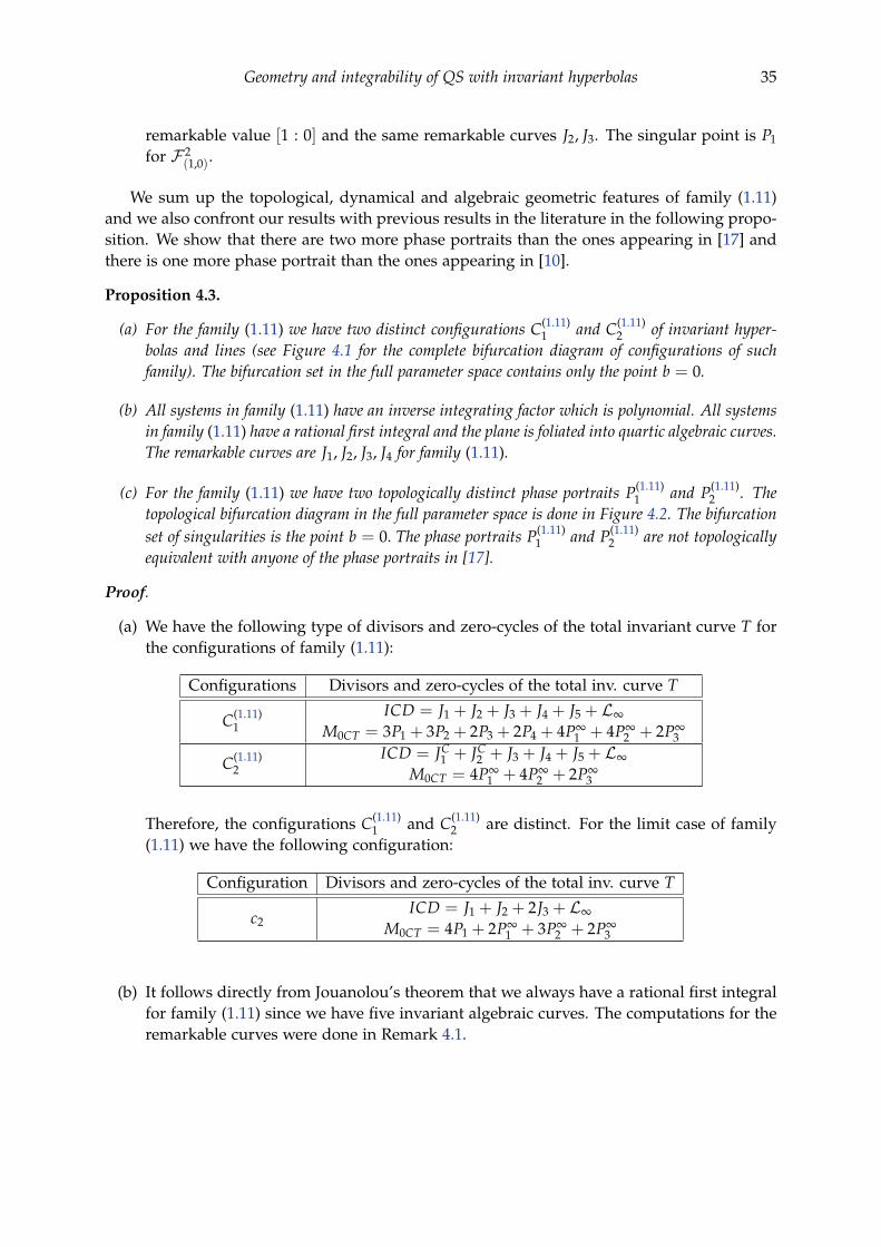
Geometry and integrability of QS with invariant hyperbolas 35
remarkable value [1 : 0] and the same remarkable curves J2, J3. The singular point is P1
for F 2(1,0).
We sum up the topological, dynamical and algebraic geometric features of family (1.11)and we also confront our results with previous results in the literature in the following propo-sition. We show that there are two more phase portraits than the ones appearing in [17] andthere is one more phase portrait than the ones appearing in [10].
Proposition 4.3.
(a) For the family (1.11) we have two distinct configurations C(1.11)1 and C(1.11)
2 of invariant hyper-bolas and lines (see Figure 4.1 for the complete bifurcation diagram of configurations of suchfamily). The bifurcation set in the full parameter space contains only the point b = 0.
(b) All systems in family (1.11) have an inverse integrating factor which is polynomial. All systemsin family (1.11) have a rational first integral and the plane is foliated into quartic algebraic curves.The remarkable curves are J1, J2, J3, J4 for family (1.11).
(c) For the family (1.11) we have two topologically distinct phase portraits P(1.11)1 and P(1.11)
2 . Thetopological bifurcation diagram in the full parameter space is done in Figure 4.2. The bifurcationset of singularities is the point b = 0. The phase portraits P(1.11)
1 and P(1.11)2 are not topologically
equivalent with anyone of the phase portraits in [17].
Proof.
(a) We have the following type of divisors and zero-cycles of the total invariant curve T forthe configurations of family (1.11):
Configurations Divisors and zero-cycles of the total inv. curve T
C(1.11)1
ICD = J1 + J2 + J3 + J4 + J5 + L∞
M0CT = 3P1 + 3P2 + 2P3 + 2P4 + 4P∞1 + 4P∞
2 + 2P∞3
C(1.11)2
ICD = JC1 + JC
2 + J3 + J4 + J5 + L∞
M0CT = 4P∞1 + 4P∞
2 + 2P∞3
Therefore, the configurations C(1.11)1 and C(1.11)
2 are distinct. For the limit case of family(1.11) we have the following configuration:
Configuration Divisors and zero-cycles of the total inv. curve T
c2ICD = J1 + J2 + 2J3 + L∞
M0CT = 4P1 + 2P∞1 + 3P∞
2 + 2P∞3
(b) It follows directly from Jouanolou’s theorem that we always have a rational first integralfor family (1.11) since we have five invariant algebraic curves. The computations for theremarkable curves were done in Remark 4.1.

36 R. Oliveira, D. Schlomiuk and A. M. Travaglini
(c) We have that:
Phase Portraits Sing. at ∞ Finite sing. Separatrix connections
P(1.11)1 (N, N, S) (n, s, s, n) 3SC f
f 6SC∞f 0SC∞
∞
P(1.11)2 (N, N, S) (©, ©, ©, ©) 0SC f
f 0SC∞f 2SC∞
∞
Therefore, we have two distinct phase portraits for systems (1.11). For the limit case offamily (1.11) we have the following phase portrait:
Phase Portrait Sing. at ∞ Finite sing. Separatrix connections
p2 (N, N, S) hpphpp(4) 0SC ff 6SC∞
f 0SC∞∞
Note that P(1.11)1
∼=top p1 and P(1.11)2
∼=top P(1.10)3 . We saw in the study of the previous
family that P(1.10)3 is not topologically equivalent with anyone if the phase portraits in
[17].
On the table below we list the phase portraits of Llibre–Yu in [17] that admit 3 singularpoints at infinity with the type (N, N, S) and with 4 real singular points in the finiteregion.
Phase Portrait Sing. at ∞ Real finite sing. Separatrix connections
R5 (N, S, N) (s, n, n, s) 4SC ff 6SC∞
f 0SC∞∞
R8, Ω1 (N, S, N) (s, n, n, s) 4SC ff 6SC∞
f 0SC∞∞
Therefore, the phase portraits P(1.11)1 is not topologically equivalent with anyone of the
phase portraits in [17]. It is however a phase portrait of systems possessing an invariantline and an invariant hyperbola.
b
(1)
(1)
(1)
(1)(1)
(1)
(1) (1)
(1)
(1)
0
(4)
2
(1)
(1)
(1)
c2C(1.11)
1 C(1.11)2
Figure 4.1: Bifurcation diagram of configurations for family (1.11). At b = 0 thetwo hyperbolas become reducible into the lines x = 0, x − y = 0 and x = 0,y = 0.

Geometry and integrability of QS with invariant hyperbolas 37
p2
b0
P(1.11)1 P(1.11)
2
Figure 4.2: Topological bifurcation diagram for family (1.11). The only bifurca-tion point is at b = 0 where all 4 singularities (real on the left or complex on theright) coalesce with (0, 0).
5 Geometric analysis of family (1.12)
Consider the family
(1.12)
x = 2a + gx2 + xy
y = a(2g− 1) + (g− 1)xy + y2, where a(g− 1) 6= 0.
This is a two parameter family depending on (a, g) ∈ R2\(0, 1). Every system in thefamily (1.12) is endowed with at least one invariant hyperbola J1 with cofactor α1 given by
J1 = a + xy, α1 = (−1 + 2g)x + 2y.
Except for a denumerable set of lines in the parameter space, i.e. except for
Lk : 2g− k = 0, k ∈N = 0, 1, 2, . . . and L : 4g− 1 = 0,
systems in (1.12) are not Liouvillian integrable (see [19]). It thus remains to be shown whathappens on these lines and we consider here the case L1 and L.
Straightforward calculations lead us to the tables listed below. The multiplicities of eachinvariant straight line and invariant hyperbola appearing in the divisor ICD of invariant al-gebraic curves were calculated by using for lines the 1st and for hyperbola the 2nd extacticpolynomial, respectively.
(i) ag(g− 1)(2g− 1)(4g− 1) 6= 0.
In [19] it is proved that except for the denumerable set of lines ∪k∈NLk ∪ L,
Lk = (a, g) ∈ R2\(0, 1) : 2g− k = 0, k ∈N,
L = (a, g) ∈ R2\(0, 1) : 4g− 1 = 0
systems (1.12) are neither Darboux nor Liouvillian integrable. We prove below thatwhen (a, g) ∈ L1 systems (1.12) are generalized Darboux integrable and when (a, g) ∈ Lsystems (1.12) are Liouvillian integrable. The cases where (a, g) ∈ ∪k∈NLk − L1 are stillopen. For these cases we were not able to prove the non-integrability and we also couldnot find other invariant algebraic curves, which we managed to search up to degree four.Although we are unable to guarantee the existence of a first integral in ∪k∈NLk − L1, itis still possible to obtain the complete topological bifurcation diagram of this family.

38 R. Oliveira, D. Schlomiuk and A. M. Travaglini
Inv. curves and cofactors Singularities Intersection points
J1 = a + xy
α1 = (−1 + 2g)x + 2y
P1 =(−2i√
a, i(2√
ag−√
a))
P2 =(2i√
a,−i(2√
ag−√
a))
P3 =(− i√
a√g ,−i
√a√
g)
P4 =(
i√
a√g , i√
a√
g)
P∞1 = [0 : 1 : 0]
P∞2 = [1 : 0 : 0]
For a < 0 we have
f , f , ©, ©; (02)SN, S if g < 0
f , f , s, s; (02)SN, N if 0 < g < 7
32n, n, s, s; (0
2)SN, N if 732 ≤ g < 1
4s, s, n, n; (0
2)SN, N if g > 14
For a > 0 we have
©, ©, n, n; (02)SN, S if g < 0
©, ©, ©, ©; (02)SN, N if g > 0
J1 ∩ L∞ =
P∞
1 simpleP∞
2 simple
Divisor and zero-cycles Degree
ICD = J1 + L∞
M0CS =
P1 + P2 + PC
3 + PC4 + 2P∞
1 + P∞2 if a < 0 and g < 0
P1 + P2 + P3 + P4 + 2P∞1 + P∞
2 if a < 0 and g > 0PC
1 + PC2 + P3 + P4 + 2P∞
1 + P∞2 if a > 0 and g < 0
PC1 + PC
2 + PC3 + PC
4 + 2P∞1 + P∞
2 if a > 0 and g > 0
T = ZJ1 = 0
M0CT =
2P∞
1 + 2P∞2 if ag > 0
P3 + P4 + 2P∞1 + 2P∞
2 if ag < 0
2
7777
3
46
(ii) ag(g− 1)(2g− 1)(4g− 1) = 0.
(ii.1) g = 0 and a 6= 0.
Under this condition, (a, g) ∈ L0 which corresponds to an open case regarding theintegrability.

Geometry and integrability of QS with invariant hyperbolas 39
Invariant curves and cofactors Singularities Intersection points
J1 = a + xy
α1 = −x + 2y
P1 =(2i√
a,−i√
a)
P2 =(2i√
a, i√
a)
P∞1 = [0 : 1 : 0]
P∞2 = [1 : 0 : 0]
f , f ; (02)SN, (1
2)S if a < 0©, ©; (0
2)SN, (12)N if a > 0
J1 ∩ L∞ =
P∞
1 simpleP∞
2 simple
Divisor and zero-cycles Degree
ICD = J1 + L∞
M0CS =
P1 + P2 + 2P∞
1 + 3P∞2 if a < 0
PC1 + PC
2 + 2P∞1 + 3P∞
2 if a > 0
T = ZJ1 = 0
M0CT =
P1 + P2 + 2P∞
1 + 2P∞2 if a < 0
2P∞1 + 2P∞
2 if a > 0
2
77
3
64
(ii.2) g = 12 and a 6= 0.
Here we have an additional invariant line which is simple and the invariant hyperbolabecomes double so we compute the exponential factor E3.
Inv.cur./exp.fac. and cofactors Singularities Intersection points
J1 = yJ2 = a + xy
E3 = e−a(g1−g0)+g1xy−2g0y2
2(a+xy)
α1 = x2 + y
α2 = 2yα3 = −g0y
P1 =(−2i√
a, 0)
P2 =(2i√
a, 0)
P3 =(−i√
2√
a,− i√
a√2
)P4 =
(i√
2√
a, i√
a√2
)P∞
1 = [0 : 1 : 0]P∞
2 = [1 : 0 : 0]
s, s, n, n; (02)SN, N if a < 0
©, ©, ©, ©; (02)SN, N if a > 0
J1 ∩ J2 = P∞2 double
J1 ∩ L∞ = simple
J2 ∩ L∞ =
P∞
1 simpleP∞
2 simple
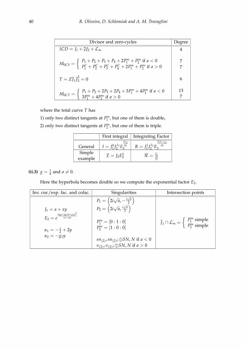
40 R. Oliveira, D. Schlomiuk and A. M. Travaglini
Divisor and zero-cycles Degree
ICD = J1 + 2J2 + L∞
M0CS =
P1 + P2 + P3 + P4 + 2P∞
1 + P∞2 if a < 0
PC1 + PC
2 + PC3 + PC
4 + 2P∞1 + P∞
2 if a > 0
T = ZJ1 J22 = 0
M0CT =
P1 + P2 + 2P3 + 2P4 + 3P∞
1 + 4P∞2 if a < 0
3P∞1 + 4P∞
2 if a > 0
4
77
6
137
where the total curve T has
1) only two distinct tangents at P∞1 , but one of them is double,
2) only two distinct tangents at P∞2 , but one of them is triple.
First integral Integrating Factor
General I = J01 Jλ2
2 E2λ2g0
3 R = J11 Jλ2
2 E2(2+λ2)
g03
Simpleexample
I = J2E23 R = J1
J22
(ii.3) g = 14 and a 6= 0.
Here the hyperbola becomes double so we compute the exponential factor E2.
Inv. cur./exp. fac. and cofac. Singularities Intersection points
J1 = a + xy
E2 = eag0+g0xy+g1y2
(a+xy)
α1 = − x2 + 2y
α2 = −g1y
P1 =(
2i√
a,− i√
a2
)P2 =
(2i√
a, i√
a2
)P∞
1 = [0 : 1 : 0]P∞
2 = [1 : 0 : 0]
sn(2), sn(2); (02)SN, N if a < 0
©(2), ©(2); (02)SN, N if a > 0
J1 ∩ L∞ =
P∞
1 simpleP∞
2 simple

Geometry and integrability of QS with invariant hyperbolas 41
Divisor and zero-cycles Degree
ICD = 2J1 + L∞
M0CS =
2P1 + 2P2 + 2P∞
1 + P∞2 if a < 0
2PC1 + 2PC
2 + 2P∞1 + P∞
2 if a > 0
T = ZJ21 = 0
M0CT =
2P1 + 2P2 + 3P∞
1 + 3P∞2 if a < 0
3P∞1 + 3P∞
2 if a > 0
3
77
5
106
where the total curve T has only two distinct tangents at P∞1 (and P∞
2 ), but one of themis double.
First integral Integrating Factor
General I = 12
(2√
2aDawsonF( √
2y√a+xy
)+x√
a+xy)(
eag0+g0xy+g1y2
a+xy
) 2g1
R = J− 1
21 E
2g12
Simpleexample
I = 12
(2√
2aDawsonF( √
2y√a+xy
)+x√
a+xy)(
ey2
a+xy
)2
R = J− 1
21 E2
2
(ii.4) g = 1 and a 6= 0.
Here we have, apart from a simple hyperbola, two additional invariant lines (real orcomplex, depending on the sign of the parameter a).
Invariant curves and cofactors Singularities Intersection points
J1 = 1− iy√a
J2 = 1 + iy√a
J3 = a + xy
α1 = y− i√
aα2 = y + i
√a
α3 = x + 2y
P1 =(−i√
a,−i√
a)
P2 =(i√
a, i√
a)
P3 =(−2i√
a, i√
a)
P4 =(2i√
a,−i√
a)
P∞1 = [0 : 1 : 0]
P∞2 = [1 : 0 : 0]
n, n, s, s; (02)SN, N if a < 0
©, ©, ©, ©; (02)SN, N if a > 0
J1 ∩ J2 = P∞2 simple
J1 ∩ J3 =
P1 simpleP∞
2 simpleJ1 ∩ L∞ = P∞
2 simple
J2 ∩ J3 =
P2 simpleP∞
2 simpleJ2 ∩ L∞ = P∞
2 simple
J3 ∩ L∞ =
P∞
1 simpleP∞
2 simple

42 R. Oliveira, D. Schlomiuk and A. M. Travaglini
Divisor and zero-cycles Degree
ICD =
J1 + J2 + J3 + L∞ if a < 0JC1 + JC
2 + J3 + L∞ if a > 0
M0CS =
P1 + P2 + P3 + P4 + 2P∞
1 + P∞2 if a < 0
PC1 + PC
2 + PC3 + PC
4 + 2P∞1 + P∞
2 if a > 0
T = ZJ1 J2 J3 = 0
M0CT =
2P1 + 2P2 + P3 + P4 + 2P∞
1 + 4P∞2 if a < 0
2P∞1 + 4P∞
2 if a > 0
44
77
5
126
where the total curve T has four distinct tangents at P∞2 .
First integral Integrating Factor
General I =(√
a + y2 + y)−√ a+y2
a√a+y2 e
√a+y2
a (x−y)a+xy R = J
121 J
122 J−2
3
Simpleexample
I =(√
a + y2 + y)−√ a+y2
a√a+y2 e
√a+y2
a (x−y)a+xy R = J
121 J
122 J−2
3
(ii.5) a = 0 and g 6= 0, 1.
Under this condition, systems (1.12) do not belong to QSH, but we study them seekinga complete understanding of the bifurcation diagram of the systems in the full family(1.12). All the affine invariant lines are y = 0 that is simple and x = 0 that is doubleso we compute the exponential factor E3. By perturbing the reducible conic xy = 0 weproduce the hyperbola a + xy = 0.
Inv. cur./exp. fac. and cofactors Singularities Intersection points
J1 = yJ2 = xE3 = e
g0x+g1yx
α1 = (−1 + g)x + yα2 = gx + yα3 = −g1y
P1 = (0, 0)
P∞1 = [0 : 1 : 0]
P∞2 = [1 : 0 : 0]
epep(4); (02)SN, S if g < 0
phph(4); (02)SN, N if g > 0
J1 ∩ J2 = P1 simpleJ1 ∩ L∞ = P∞
2 simpleJ2 ∩ L∞ = P∞
1 simple
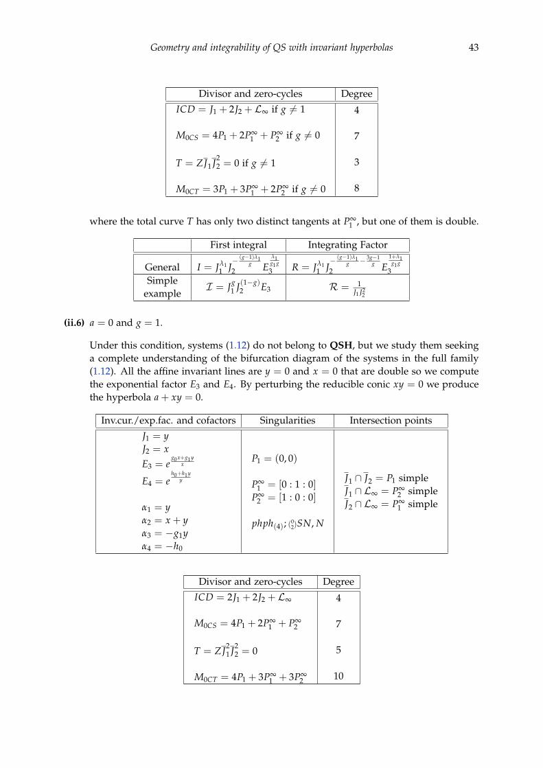
Geometry and integrability of QS with invariant hyperbolas 43
Divisor and zero-cycles Degree
ICD = J1 + 2J2 + L∞ if g 6= 1
M0CS = 4P1 + 2P∞1 + P∞
2 if g 6= 0
T = ZJ1 J22 = 0 if g 6= 1
M0CT = 3P1 + 3P∞1 + 2P∞
2 if g 6= 0
4
7
3
8
where the total curve T has only two distinct tangents at P∞1 , but one of them is double.
First integral Integrating Factor
General I = Jλ11 J− (g−1)λ1
g2 E
λ1g1g
3 R = Jλ11 J− (g−1)λ1
g − 3g−1g
2 E1+λ1g1g
3Simple
exampleI = Jg
1 J(1−g)2 E3 R = 1
J1 J22
(ii.6) a = 0 and g = 1.
Under this condition, systems (1.12) do not belong to QSH, but we study them seekinga complete understanding of the bifurcation diagram of the systems in the full family(1.12). All the affine invariant lines are y = 0 and x = 0 that are double so we computethe exponential factor E3 and E4. By perturbing the reducible conic xy = 0 we producethe hyperbola a + xy = 0.
Inv.cur./exp.fac. and cofactors Singularities Intersection points
J1 = yJ2 = xE3 = e
g0x+g1yx
E4 = eh0+h1y
y
α1 = yα2 = x + yα3 = −g1yα4 = −h0
P1 = (0, 0)
P∞1 = [0 : 1 : 0]
P∞2 = [1 : 0 : 0]
phph(4); (02)SN, N
J1 ∩ J2 = P1 simpleJ1 ∩ L∞ = P∞
2 simpleJ2 ∩ L∞ = P∞
1 simple
Divisor and zero-cycles Degree
ICD = 2J1 + 2J2 + L∞
M0CS = 4P1 + 2P∞1 + P∞
2
T = ZJ21 J2
2 = 0
M0CT = 4P1 + 3P∞1 + 3P∞
2
4
7
5
10

44 R. Oliveira, D. Schlomiuk and A. M. Travaglini
where the total curve T has only two distinct tangents at P∞1 (and P∞
2 ), but one of themis double.
First integral Integrating Factor
General I = Jλ11 J0
2 Eλ1g13 E0
4 R = Jλ11 J−2
2 E1+λ1
g13 E0
4Simple
exampleI = J1E3 R = 1
J1 J22
(ii.7) a = g = 0.
Under this condition, systems (1.12) do not belong to QSH, but we study them seekinga complete understanding of the bifurcation diagram of the systems in the full family(1.12). The line y = 0 is filled up with singularities, therefore this is a degenerate system.The following study is done with the reduced system. For this system the line x = 0 isdouble so we compute the exponential factor E2.
Inv.cur./exp.fac. and cofactors Singularities Intersection points
J1 = xE2 = e
g0x+g1yx
α1 = 1α2 = −g1
P1 = (0, 0)
P∞1 = [0 : 1 : 0]
([|]; nd); (02)SN, ([|]; ∅)
J1 ∩ L∞ = P∞1 simple
Divisor and zero-cycles Degree
ICD = 2J1 + L∞
M0CS = P1 + 2P∞1
T = ZJ21 = 0
M0CT = 2P1 + 3P∞1
3
3
3
5
where the total curve T has only two distinct tangents at P∞1 , but one of them is double.
First integral Integrating Factor
General I = Jg1λ21 Eλ2
2 R = J−2+g1λ21 Eλ2
2Simple
exampleI = J1E2 R = 1
J21
We sum up the topological, dynamical and algebraic geometric features of family (1.12)and also confront our results with previous results in literature in the following propo-sition. We show that there are two more phase portraits than the ones appearing in[17].

Geometry and integrability of QS with invariant hyperbolas 45
Proposition 5.1.
(a) For the family (1.12) we obtained seven distinct configurations C(1.12)1 −C(1.12)
7 of invariant hyper-bolas and lines (see Figure 5.1 for the complete bifurcation diagram of configurations of this fam-ily). The bifurcation set of configurations in the full parameter space is ag(g− 1)(g− 1/2)(g−1/4) = 0. On (g− 1/2)(g− 1/4) = 0 the invariant hyperbola is double. On g = 1/2 we havean additional invariant line and on g = 1 we have two additional invariant lines. On g = 0 wejust have a simple invariant hyperbola. On a = 0 the hyperbola becomes reducible into two linesand when a = g = 0 one of the lines is filled up with singularities.
(b) The family (1.12) is generalized Darboux integrable when g = 1/2 and it is Liouvillian integrablewhen g = 1/4.
(c) For the family (1.12) we have seven topologically distinct phase portraits P(1.12)1 − P(1.12)
7 . Thetopological bifurcation diagram of family (1.12) is done in Figure 5.2. The bifurcation set are thehalf lines g = 1/4 and g = 1/2 with a < 0 and the lines g = 0 and a = 0. The half lineg = 1/4 with a < 0 and the lines g = 0, a = 0 are bifurcation sets of singularities and thehalf line g = 1/2 with a < 0 is a bifurcation of saddle to saddle connection. The phase portraitsP(1.12)
4 and P(1.12)6 are not topologically equivalent with anyone of the phase portraits in [17].
Proof.
(a) We have the following type of divisors and zero-cycles of the total invariant curve T forthe configurations of family (1.12):
Configurations Divisors and zero-cycles of the total inv. curve T
C(1.12)1
ICD = J1 + L∞
M0CT = P3 + P4 + 2P∞1 + P∞
2
C(1.12)2
ICD = J1 + L∞
M0CT = 2P∞1 + P∞
2
C(1.12)3
ICD = J1 + L∞
M0CT = 2P∞1 + P∞
2
C(1.12)4
ICD = J1 + 2J2 + L∞
M0CT = P1 + P2 + 2P3 + 2P4 + 3P∞1 + 4P∞
2
C(1.12)5
ICD = J1 + 2J2 + L∞
M0CT = 3P∞1 + 4P∞
2
C(1.12)6
ICD = 2J1 + L∞
M0CT = 2P1 + 2P2 + 3P∞1 + 3P∞
2
C(1.12)7
ICD = 2J1 + L∞
M0CT = 3P∞1 + 3P∞
2
Therefore, the configurations C(1.12)1 up to C(1.12)
7 are all distinct. For the limit cases offamily (1.12) we have the following configurations:

46 R. Oliveira, D. Schlomiuk and A. M. Travaglini
Configurations Divisors and zero-cycles of the total inv. curve T
c3ICD = J1 + 2J2 + L∞
M0CT = 3P1 + 3P∞1 + 2P∞
2
c4ICD = 2J1 + 2J2 + L∞
M0CT = 4P1 + 3P∞1 + 3P∞
2
c5ICD = 2J1 + L∞
M0CT = 2P1 + 3P∞1
c6ICD = J1 + J2 + J3 + L∞
M0CT = 2P1 + 2P2 + P3 + P4 + 2P∞1 + 4P∞
2
c7ICD = JC
1 + JC2 + J3 + L∞
M0CT = 2P∞1 + 4P∞
2
(b) This is shown in the previously exhibited tables.
(c) We have that:
Phase Portraits Sing. at ∞ Finite sing. Separatrix connections
P(1.12)1 ((0
2)SN, N) (n, n, s, s) 2SC ff 6SC∞
f 0SC∞∞
P(1.12)2 ((0
2)SN, N) (s, s, n, n) 4SC ff 6SC∞
f 0SC∞∞
P(1.12)3
((02)SN, S)
((02)SN, (1
2)S)( f , f , ©, ©)
( f , f )0SC f
f 2SC∞f 2SC∞
∞
P(1.12)4
((02)SN, N)
((02)SN, N)
((02)SN, (1
2)N)
(©, ©, ©, ©)
(©(2), ©(2))
(©, ©)
0SC ff 0SC∞
f 2SC∞∞
P(1.12)5 ((0
2)SN, S) (©, ©, n, n) 0SC ff 2SC∞
f 0SC∞∞
P(1.12)6 ((0
2)SN, N) (s, s, n, n) 3SC ff 6SC∞
f 0SC∞∞
P(1.12)7 ((0
2)SN, N) (sn(2), sn(2)) 0SC ff 6SC∞
f 0SC∞∞
Therefore, we have seven distinct phase portraits for systems (1.12). For the limit casesof family (1.12) we have the following phase portraits:
Phase Portraits Sing. at ∞ Finite sing. Separatrix connections
p3 ((02)SN, N) phph(4) 0SC f
f 4SC∞f 0SC∞
∞
p4 (02)SN, ([|]; ∅) ([|]; nd) 0SC f
f 2SC∞f 0SC∞
∞
p5 ((02)SN, S) epep(4) 0SC f
f 4SC∞f 0SC∞
∞
On the table below we list all the phase portraits of Llibre-Yu in [17] that admit 2 singularpoints at infinity with the type (SN, N):

Geometry and integrability of QS with invariant hyperbolas 47
Phase Portrait Sing. at ∞ Real finite sing. Separatrix connections
L01 (SN, N) ∅ 0SC ff 0SC∞
f 3SC∞∞
L03 (SN, N) ∅ 0SC ff 0SC∞
f 3SC∞∞
ω1 (SN, N) (s, n) 1SC ff 6SC∞
f 0SC∞∞
The phase portraits P(1.12)4 and P(1.12)
6 are not topologically equivalent with anyone ofthe phase portraits in [17]. They are however phase portraits of systems possessing aninvariant line and an invariant hyperbola (when g = 1/2).
Remark 5.2. The family (1.12) does not have any case where the inverse integrating factor ispolynomial. We just have a polynomial inverse integrating factor on the limit case a = 0 offamily (1.12).
a = 0
g = 1/4
g = 1/2
g = 1
(2)
(1)(1)
(1)
(2)
(1)(4)
(2)
(2)
(1)(4)
c3
c4
c5
c6 c7
c3
c3
c3
c3
c3
(2)
(2,1)
(2)
(1)
(1)
(2)
(1)
(1)(1)
(1)2
2
2
2
2
(2)
2(2)
(2)(1)
(2)
(1)(1)
(1)
(1)
(2)
(1)
(2)2
(1)
2
(2)
g = 0
c3
(1)
(2)
(1)
(2)
(1)(1)
(1)(1)
C(1.12)1
C(1.12)1
C(1.12)1
C(1.12)1
C(1.12)3
C(1.12)2 C(1.12)
2
C(1.12)3
C(1.12)3
C(1.12)3
C(1.12)3
C(1.12)1
C(1.12)4 C(1.12)
5
C(1.12)6 C(1.12)
7
(2,1)
(2)
Figure 5.1: Bifurcation diagram of configurations for family (1.12): In this figureon the dashed line a = 0 the hyperbola becomes reducible into two lines x = 0and y = 0. When a = g = 0 the line y = 0 is filled up with singularities. For thebifurcation curves we either have an additional line or coalescing hyperbolas ora change in the multiplicity of a infinity singularity. On the dashed line g = 1we have two additional lines. The dashed lines represent complex lines.
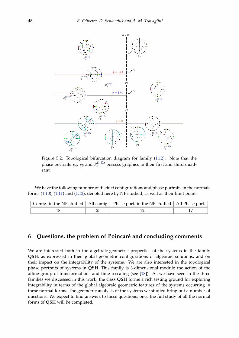
48 R. Oliveira, D. Schlomiuk and A. M. Travaglini
a = 0
g = 1/4
g = 1/2
p3
p3
p3
p4
p4p5
p4p3
p4p3P(1.12)
2
P(1.12)2
g = 0P(1.12)
1
P(1.12)3
P(1.12)3
P(1.12)4
P(1.12)4
P(1.12)5
P(1.12)6
P(1.12)7
Figure 5.2: Topological bifurcation diagram for family (1.12). Note that thephase portraits p4, p5 and P(1.12)
3 possess graphics in their first and third quad-rant.
We have the following number of distinct configurations and phase portraits in the normalsforms (1.10), (1.11) and (1.12), denoted here by NF studied, as well as their limit points:
Config. in the NF studied All config. Phase port. in the NF studied All Phase port.
18 25 12 17
6 Questions, the problem of Poincaré and concluding comments
We are interested both in the algebraic-geometric properties of the systems in the familyQSH, as expressed in their global geometric configurations of algebraic solutions, and ontheir impact on the integrability of the systems. We are also interested in the topologicalphase portraits of systems in QSH. This family is 3-dimensional modulo the action of theaffine group of transformations and time rescaling (see [18]). As we have seen in the threefamilies we discussed in this work, the class QSH forms a rich testing ground for exploringintegrability in terms of the global algebraic geometric features of the systems occurring inthese normal forms. The geometric analysis of the systems we studied bring out a number ofquestions. We expect to find answers to these questions, once the full study of all the normalforms of QSH will be completed.

Geometry and integrability of QS with invariant hyperbolas 49
6.1 The problem of Poincaré
For two out of the three families discussed in this work we have an answer to Poincaré’sproblem of algebraic integrability for each one of the systems in these families. The answer isgiven entirely in geometric terms (see Theorem 3.6 in Subsection 3.1) and all systems in thefamily (1.11) are algebraically integrable. This raises the following question: For how manyof the remaining normal forms could we solve the problem of Poincaré for all the systemsin the families defined by their respective normal forms? Could this problem be solved ingeometrical terms as it was possible for the normal form (A)?
6.2 The problem of generalizing the Christopher–Kooij Theorem 1.15
We saw that under the “generic” conditions of Christopher and Kooij (C–K), formulated al-gebraically on the algebraic invariant curves f1(x, y), . . . , fk(x, y) of a polynomial differentialsystem, we are assured to have a polynomial inverse integrating factor of the special form
f1(x, y) . . . fk(x, y).
In this article we see cases where these “generic conditions” of (C–K) are not satisfied andyet we still have an integrating factor which is polynomial. Furthermore, in some cases, thispolynomial inverse integrating factor is of the same form as the one in the (C–K) theorem.Here are some examples occurring in the families we considered.
(I) For the family (1.10).
(1) All the systems in family (1.10) have an inverse integrating factor which is polynomial, theyare Darboux integrable and have in the generic case only two invariant lines J1, J2 and twoinvariant hyperbolas J3, J4. An inverse polynomial factor is J1 J2 J3 J4 just like in C–K theorem.The condition (a) of the C–K theorem 1.15 is satisfied since our curves are lines and hyperbolasand they are, of course, non-singular and irreducible. The condition (b) is also satisfied sincethe coefficients in M0ST are all equal to 2. The condition (c) is not satisfied because both ofthe hyperbolas J3 and J4 intersect the line at infinity at P∞
1 and they are tangent at this point.The condition (d) is not satisfied because the sum of the degrees of the curves is 6 and not 3.However, the conclusion is the same as in theorem 1.15.
(2) In the non-generic cases (a− 3v2/4)(a + 3v2)(a− 8v2/9) = 0 we have a similar situationand an inverse polynomial integrating factor. We have, as in the generic case, the two invariantlines J1, J2 and we have, apart from the two invariant hyperbolas J4, J5 and additional invariantcurve J3. We again have (a) and (b) satisfied but not (c) and (d) of (C–K) theorem 1.15.However, if we restrict our attention only to the remarkable curves J1, J2, J4, J5 then we stillhave an inverse integrating factor of the form J1 J2 J4 J5 as in the (C–K) theorem.
(II) Consider now the family (1.11).
(1) The systems in the family (1.11) have in the generic case three invariant lines J1, J2, J3 andtwo invariant hyperbolas J4, J5. Let us now consider for our discussion only the remarkablecurves, the three lines J1, J2, J3 and the hyperbola J4. These of course satisfy the conditions (a)and (b). However they do not satisfy (c) because for example J1, J2, J4 intersect at P2. They alsodo not satisfy (d). If we limit our attention to the four curves J1, J2, J3, J4 we see that we haveas an inverse integrating factor the polynomial J1 J2 J3 J4 which we get by taking in the generalexpression of the integrating factor λ1 = λ2 = λ4 = −1.

50 R. Oliveira, D. Schlomiuk and A. M. Travaglini
So we can ask the following questions:
Question 1: How should the geometry of the configuration of algebraic solutions J1, . . . , Jk ofa polynomial system be so as to have an inverse integrating factor which is polynomial? Inparticular, how should this geometry be in order to have an inverse integrating factor J1 · · · Jk?How could we relax, generalize, the hypotheses in the (C–K) theorem such that the sameconclusion holds?
Question 2: If a system has a rational first integral do we always have an inverse integratingfactor involving only remarkable curves?
Consider now the non-generic case v(a− v2) = 0 of the family (1.10). We have that oneof the invariant curves becomes double. In the case v = 0 we have two simple invariant linesJ1, J2 and one double invariant hyperbola J3. A polynomial inverse integrating factor in thiscase is J1 J2 J2
3 . In the case a− v2 = 0 we have a double line J1 and two simple hyperbolas J2, J3.We have a polynomial integrating factor J2
1 J2 J3. In this case we still have a polynomial inverseintegrating factor.
Question 3: Can we generalize the (C–K) Theorem 1.15 so as to include multiplicity? In whatcases there is a relation between the multiplicity s of an algebraic solution Ji and the exponentof Ji appearing in the polynomial inverse integrating factor?
6.3 On the bifurcation diagrams
We have two kinds of bifurcation diagrams: topological and geometrical, i.e., of geometricconfigurations of algebraic solutions (lines and hyperbolas).
Question 1: What is the relation between these two kinds of bifurcation diagrams?
In all three families the topological bifurcation set of the phase portraits is a subset of thebifurcation set of configurations of algebraic solutions. This inclusion is strict for the first andlast families.
The bifurcation set BifA for topological phase portraits in the family (A) is formed by thehalf-line of v = 0, a < 0 ((BifA)
(1)); the non-zero points on the parabola a = v2 ((BifA)(2)).
On (BifA)(1) and on (BifA)
(2) 4 real finite singular points coalesce into 2 real finite doublepoints. In the first case, after crossing the half-line they split again into 4 real singular points,while in the second case they split into 4 complex finite singular points which are finitepoints of intersection of the complexifications of each one of two real hyperbolas with the twocomplex invariant lines, respectively.
It is interesting to observe that these topological bifurcation points have an impact onthe bifurcation set of geometrical configurations. Indeed, first we mention that above andbelow the half-line v = 0 and a < 0 we have two couples of real singularities, the points ineach couple are located on distinct branches of one hyperbola. When two singular points ondifferent hyperbolas coalesce this yields the coalescence of the respective branches and also ofthe two hyperbolas, producing a double hyperbola.
On the non-zero points of the parabola a = v2 the coalescence of the 4 real finite singularpoints into two couples of double real singular points yields the coalescence of the two linesinto a double real line which afterwards splits into two complex lines. In this case again wesee that the topological bifurcation points produce also bifurcations in the configurations.
We note that we have a saddle to saddle connection on the parabola a = v2 for (a, v) 6=(0, 0).
Geometry and integrability of QS with invariant hyperbolas 51
On the bifurcation points situated on the remaining three parabolas we either have theoccurrence of an additional hyperbola (on a− 8v2/9 = 0 or on a + 3v2 = 0) or the appearanceof an additional invariant line (on a− 3v2/4 = 0). The presence of these additional invariantcurves does not affect in any way the bifurcation diagram of the systems.
In conclusion we have:
(i) Impact of the topological bifurcations on the bifurcations of configurations: The bifurcationpoints of singularities of the systems located on the algebraic solutions, when real singularpoints become multiple, become also bifurcation points for the multiplicity of the algebraicsolutions, inducing coalescence of the respective curves and hence of their geometric configu-ration.
(ii) The bifurcation points of configurations due to the appearance of additional invariantcurves (three hyperbolas instead of two or three lines instead of two lines) have no conse-quence for the topological bifurcation diagram of this family.
(iii) Inside the parabola a = v2 i.e. for points (a, v) such that v2− a < 0 where we have complexsingularities, we have no bifurcation points of phase portraits but we have, on the half-linev = 0, a > 0 bifurcation points of configurations, the two hyperbolas coalescing into a doublehyperbola. Here we need to stress the fact that on this half-line we have two double complexsingularities and while this fact has no impact on the topological bifurcation it is important forthe bifurcations of the configurations. Indeed, when the four complex singularities becometwo double complex singularities on this half-line, the two hyperbolas on which they are lyingcoalesce becoming a double hyperbola.
Limit points of the bifurcation diagram for (A) Let us discuss the bifurcation phenomenawhich occur at the limiting points of our parameter space for systems in the family (A), i.e.the points on a = 0. The topological bifurcation on this line is easy to understand. Indeed,except for the the point (0, 0) where all four singularities collide, all the other points on a = 0are bifurcation points of saddle to saddle connections. All the points on the line a = 0 arealso points of bifurcation of configurations of algebraic solutions. However this bifurcationis a bit harder to understand. Indeed, at these points say on v > 0 we have a configurationwith three simple affine invariant lines, the vertical line intersecting the two parallel lines attwo points and forming a saddle-to saddle connection. It is clear that this configuration splitsinto the configuration C(1.10)
1 on the left which has two hyperbolas and two invariant lines. Soin some sense the configuration on a = 0 should be considered as a multiple configuration sinceit yields new algebraic solutions. Analyzing the bifurcation phenomenon we see that eachone of the two hyperbolas splits into two lines on a = 0 and v > 0. Indeed, the hyperbolaJ4 splits into the line x = 0 and the line J1 and the hyperbola J3 splits into J2 and x = 0. Sothat although for a = 0 each one of the lines is simple, each line contributes to the multiplicityof the configuration. Considering the composite cubic curve xJ1 J2 = 0 we may say that thisconfiguration has (geometric) multiplicity two in this family as it splits into two cubic curvesJ1 J4 and J2 J3. On the other hand we see that we have on a = 0 an exponential factor involvingin its exponent at the denominator of the rational function, the polynomial xJ1 J2 which turnsout to be of integrable multiplicity two. The notions of integrable multiplicity and geometricmultiplicity in [9] are not restricted to algebraic solutions. But the authors say there clearlythat the equivalence between integrable and geometric multiplicities occurs only for integrablesolutions. In the above family these two multiplicities coincide. So we have the following
Question: Under what condition on (finite) configurations of algebraic solutions do the twomultiplicities, integrable and geometric coincide?

52 R. Oliveira, D. Schlomiuk and A. M. Travaglini
Finally we note that the point (0, 0) produces in perturbations all nine configurationswhich we encounter in the extension of the family (A), apart from the fact that we are in-terested in producing all the phase portraits of family QSH as well as fully understanding theintegrability of this family, the questions raised above are additional motivation for complet-ing the study of this family.
7 Appendix
Considering r = m1/m2 where m1, m2 ∈ Z we can say that
I =(
J1
J2
)m2(
J3
J4
)m1
is a rational first integral of (1.10) when a = (1− (m1/m2)2)v2. Consider
F(c1,c2) = c1 Jm21 Jm1
3 − c2 Jm22 Jm1
4 = 0.
We have the following:
• Taking m1 = 2 and m2 = 4 (i.e. a = 3v2/4) we have that
F(1,1) = − 2716 v3y
(81v4 + 36v2 (−2x2 + xy + y2)+ 16x(x− y)3
).
Therefore, we have a line and a quartic as remarkable curves.
• Taking m1 = 2 and m2 = 6 (i.e. a = 8v2/9) we have that
F(1,1) =329 v3 (v2 + 3y(y− x)
) (3v4(5x− 8y)− 2v2(x− y)2(5x + 4y) + 3x(x− y)4
).
Therefore, we have a hyperbola and a quintic as remarkable curves.
• Taking m1 = 2 and m2 = 8 (i.e. a = 15v2/16) we have that
F(1,1) =27
262144 v3(36v2x− 45v2y− 80x2y + 160xy2 − 80y3)
(3645v6 + 19440v4x2 − 58320v4xy + 38880v4y2 − 11520v2x4 + 23040v2x3y
− 23040v2xy3 + 11520v2y4 + 4096x6 − 20480x5y + 40960x4y2 − 40960x3y3
+ 20480x2y4 − 4096xy5).
Therefore, we have a cubic and a polynomial of degree 6 as remarkable curves.
• Taking m1 = 3 and m2 = 6 (i.e. a = 3v2/4) we have that
F(1,1) =81512 v3y(6561v8 − 1944v6 (6x2 − 3xy− 5y2)+ 1296v4(x− y)2 (6x2 + 2xy + y2)− 1152v2x(x− y)4(2x + y) + 256x2(x− y)6).
Therefore, we have a line and a polynomial of degree 8 as remarkable curves.

Geometry and integrability of QS with invariant hyperbolas 53
• Taking m1 = 3 and m2 = 9 (i.e. a = 8v2/9) we have that
F(1,1) =1627 v3 (v2 − 3xy + 3y2) (64v10 + 675v8x2 − 2544v8xy + 2112v8y2
− 900v6x4 + 2520v6x3y− 612v6x2y2 − 2736v6xy3 + 1728v6y4
+ 570v4x6 − 2232v4x5y + 3420v4x4y2 − 2760v4x3y3 + 1530v4x2y4
− 720v4xy5 + 192v4y6 − 180v2x8 + 936v2x7y− 1836v2x6y2 + 1440v2x5y3
+ 180v2x4y4 − 1080v2x3y5 + 684v2x2y6 − 144v2xy7 + 27x10 − 216x9y
+ 756x8y2 − 1512x7y3 + 1890x6y4 − 1512x5y5 + 756x4y6 − 216x3y7 + 27x2y8).
Therefore, we have a hyperbola and a polynomial of degree 10 as remarkable curves.
• Taking m1 = 4 and m2 = 2 (i.e. a = −3v2) we have that
F(1,1) = 216v3(9v2 + xy)(405v4x− 81v4y− 45v2x3 + 63v2x2y− 18v2xy2
+ x5 − 3x4y + 3x3y2 − x2y3).
Therefore, we have a hyperbola and a quintic as remarkable curves.
• Taking m1 = 4 and m2 = 6 (i.e. a = 5v2/9) we have that
F(1,1) = − 881 v3(100v4 − 21v2x2 + 270v2xy + 75v2y2 − 45x3y + 90x2y2 − 45xy3)
(420v6x + 300v6y− 385v4x3 + 255v4x2y + 105v4xy2 + 25v4y3 + 105v2x5
+ 90x4y3 − 45x3y4 + 9x2y5).
Therefore, we have a quartic and a polynomial of degree 7 as remarkable curves.
• Taking m1 = 4 and m2 = 8 (i.e. a = 3v2/4) we have that
F(1,1) = − 272048 v3y(81v4 − 72v2x2 + 36v2xy + 36v2y2 + 16x4 − 48x3y
+ 48x2y2 − 16xy3)(6561v8 − 11664v6x2 + 5832v6xy + 17496v6y2
+ 7776v4x4 − 12960v4x3y + 3888v4x2y2 + 1296v4y4 − 2304v2x6
+ 8064v2x5y− 9216v2x4y2 + 2304v2x3y3 + 2304v2x2y4 − 1152v2xy5
+ 256x8 − 1536x7y + 3840x6y2 − 5120x5y3 + 3840x4y4 − 1536x3y5 + 256x2y6).
Therefore, we have a line, a quartic and a polynomial of degree 8 as remarkable curves.
• Taking m1 = 4 and m2 = 12 (i.e. a = 8v2/9) we have that
F(1,1) =6481 v3(v2 − 3xy + 3y2)(15v4x− 24v4y− 10v2x3 + 12v2x2y + 6v2xy2
− 8v2y3 + 3x5 − 12x4y + 18x3y2 − 12x2y3 + 3xy4)(64v10 + 225v8x2
− 1104v8xy + 960v8y2 − 300v6x4 + 840v6x3y + 180v6x2y2 − 1680v6xy3
+ 960v6y4 + 190v4x6 − 744v4x5y + 1140v4x4y2 − 920v4x3y3 + 510v4x2y4
− 240v4xy5 + 64v4y6 − 60v2x8 + 312v2x7y− 612v2x6y2 + 480v2x5y3
+ 60v2x4y4 − 360v2x3y5 + 228v2x2y6 − 48v2xy7 + 9x10 − 72x9y + 252x8y2
− 504x7y3 + 630x6y4 − 504x5y5 + 252x4y6 − 72x3y7 + 9x2y8).
Therefore, we have a hyperbola, a quintic and a polynomial of degree 10 as remarkablecurves.

54 R. Oliveira, D. Schlomiuk and A. M. Travaglini
• Taking m1 = 4 and m2 = 16 (i.e. a = 15v2/16) we have that
F(1,1) =27
2199023255552 v3(36v2x− 45v2y− 80x2y + 160xy2 − 80y3)
(3645v6 + 19440v4x2 − 58320v4xy + 38880v4y2 − 11520v2x4 + 23040v2x3y
− 23040v2xy3 + 11520v2y4 + 4096x6 − 20480x5y + 40960x4y2 − 40960x3y3
+ 20480x2y4 − 4096xy5)(13286025v12 + 383582304v10x2 − 1029814560v10xy
+ 661348800v10y2 + 293932800v8x4 − 3174474240v8x3y + 8406478080v8x2y2
− 8465264640v8xy3 + 2939328000v8y4 − 418037760v6x6 + 2090188800v6x5y
− 2090188800v6x4y2 − 4180377600v6x3y3 + 10450944000v6x2y4
− 7942717440v6xy5 + 2090188800v6y6 + 291962880v4x8 − 1804861440v4x7y
+ 4830658560v4x6y2 − 7431782400v4x5y3 + 7431782400v4x4y4
− 5202247680v4x3y5 + 2601123840v4x2y6 − 849346560v4xy7 + 132710400v4y8
− 94371840v2x10 + 660602880v2x9y− 1887436800v2x8y2 + 2642411520v2x7y3
− 1321205760v2x6y4 − 1321205760v2x5y5 + 2642411520v2x4y6
− 1887436800v2x3y7 + 660602880v2x2y8 − 94371840v2xy9 + 16777216x12
− 167772160x11y + 754974720x10y2 − 2013265920x9y3 + 3523215360x8y4
− 4227858432x7y5 + 3523215360x6y6 − 2013265920x5y7 + 754974720x4y8
− 167772160x3y9 + 16777216x2y10).
Therefore, we have a cubic, a polynomial of degree 6 and a polynomial of degree 12 asremarkable curves.
These computations suggest that the remarkable curves of algebraically integrable sys-tems in the family (A) have an unbounded degree.
Acknowledgments
The first author is partially supported by FAPESP grant number 2019/21181–0 and by CNPqgrant number 304766/2019–4. The second author is partially supported by the grant NSERCGrant RN000355. The third author was financed in part by the Coordenação de Aperfeiçoa-mento de Pessoal de Nível Superior - Brasil (CAPES) - Finance Code 001.
The authors are thankful to the referee for the corrections and comments he/she made.
References
[1] J. C. Artés, B. Grunbaum, J. Llibre, On the number of invariant straight lines for polyno-mial differential systems. Pacific J. Math. 184(1998), 317–327. https://doi.org/10.2140/pjm.1998.184.207; MR1628583
[2] J. C. Artés, J. Llibre, D. Schlomiuk, N. Vulpe, Geometric configurations of singularities ofplanar polynomial differential systems. A global classification in the quadratic case, Birkhäuser,Basel, 1st ed, 2021.

Geometry and integrability of QS with invariant hyperbolas 55
[3] J. C. Artés, J. Llibre, D. Schlomiuk, N. Vulpe, Global topological configurations ofsingularities for the whole family of quadratic differential systems, Qual. Theory Dyn. Syst.19(2020), No. 51, 1–32. https://doi.org/10.1007/s12346-020-00372-7; MR4067332
[4] J. Chavarriga, H. Giacomini, J. Giné, J. Llibre, Darboux integrability and the inverseintegrating factor, J. Differential Equations 194(2003), 116–139. https://doi.org/10.1016/S0022-0396(03)00190-6; MR2001031
[5] C. Christopher Invariant algebraic curves and conditions for a center, Proc.Roy. Soc. Edinburgh Sect. A 124(1994), No. 6, 1209–1229. https://doi.org/10.1017/S0308210500030213; MR1313199
[6] C. Christopher, R. Kooij, Algebraic invariant curves and the integrability of polyno-mial systems, Appl. Math. Lett. 6(1993), No. 4, 51–53. https://doi.org/10.1016/0893-9659(93)90123-5; MR1348232
[7] C. Christopher, J. Llibre, Algebraic aspects of integrability for polynomial sys-tems, Qual. Theory Dyn. Syst. 1(1999), 71–95. https://doi.org/10.1007/BF02969405;MR1747198
[8] C. Christopher, J. Llibre, C. Pantazi, S. Walcher, On planar polynomial vector fieldswith elementary first integrals, J. Differential Equations 267(2019), 4572–4588. https://doi.org/10.1016/j.jde.2019.05.007; MR3983046
[9] C. Christopher, J. Llibre, J. V. Pereira, Multiplicity of invariant algebraic curves inpolynomial vector fields, Pacific J. Math. 229(2007), No. 1, 1–58. https://doi.org/10.2140/pjm.2007.229.63; MR2276503
[10] B. Coll, A. Ferragut, J. Llibre, Phase portraits of the quadratic systems with a poly-nomial inverse integrating factor, Internat. J. Bifur. Chaos Appl. Sci. Engrg. 19(2008), No. 3,765–783. https://doi.org/10.1142/S0218127409023299; MR2533481
[11] G. Darboux, Mémoire sur les équations différentielles algébriques du premier ordre etdu premier degré (in French), Bull. Sci. Math. Astron. 2(1878) 60–96; 123–144; 151–200.http://www.numdam.org/item?id=BSMA_1878_2_2_1_60_1; Zbl 10.0214.01
[12] F. Dumortier, J. Llibre, J. C. Artés, Qualitative theory of planar differential systems, Univer-sitext, Springer-Verlag, New York–Berlin, 2008. https://doi.org/10.1007/978-3-540-32902-2; MR2256001
[13] F. Dumortier, R. Roussarie, C. Rousseau, Hilbert’s 16th problem for quadratic vectorfields, J. Differential Equations 110(1994), 66–133. https://doi.org/10.1006/jdeq.1994.1061; MR1275749
[14] A. Ferragut, J Llibre, On the remarkable values of the rational first integrals of polyno-mial vector fields. J. Differential Equations 241(2007), 399–417. https://doi.org/10.1016/j.jde.2007.05.002; MR2358899
[15] J. Jouanolou, Équations de Pfaff algébriques, Lectures Notes in Mathematics, Vol. 708,Springer-Verlag, 1979. https://doi.org/10.1007/BFb0063393; MR537038

56 R. Oliveira, D. Schlomiuk and A. M. Travaglini
[16] J. Llibre, X. Zhang, Darboux theory of integrability in Cn taking into account the mul-tiplicity, J. Differential Equations 246(2009), No. 2, 541–551. https://doi.org/10.1016/j.jde.2008.07.020; MR2468727
[17] J. Llibre, J. Yu, Global phase portraits for quadratic systems with a hyperbola and astraight line as invariant algebraic curves, Electron. J. Differential Equations 2018, No. 141,1–19. MR3831887
[18] R. D. S. Oliveira, A. C. Rezende, D. Schlomiuk, N. Vulpe, Geometric and algebraicclassification of quadratic differential systems with invariant hyperbolas, Electron. J. Dif-ferential Equations 2017, No. 295, 1–112. MR3748013
[19] R. D. S. Oliveira, D. Schlomiuk, A. M. Travaglini, C. Valls, Conceptual up to datesurvey of Darboux’s theory of integrability with applications of bifurcation to a family ofquadratic differential systems, preprint, 2020.
[20] J. V. Pereira Vector fields, invariant varieties and linear systems, Ann. Inst. Fourier (Greno-ble) 51(2001), No. 5, 1385–1405. https://doi.org/10.5802/aif.1858; MR1860669
[21] M. J. Prelle, M. F. Singer, Elementary first integrals of differential equations, Trans.Amer. Math. Soc. 279(1983), 215–229. https://doi.org/10.1090/S0002-9947-1983-0704611-X; MR0704611
[22] H. Poincaré, Sur l’intégration des équations différentielles du premier ordre et dupremier degré I et II, Rend. Circ. Mat. Palermo 5(1891), 161–191; Rend. Circ. Mat.Palermo 11(1897) 193–239. https://doi.org/10.1007/BF03015693 and https://doi.org/10.1007/BF03015916
[23] M. Rosenlicht, On Liouville’s theory of elementary functions, Pacific J. Math. 65(1976),485–492. https://doi.org/10.2140/pjm.1976.65.485 MR0447199
[24] D. Schlomiuk, Topological and polynomial invariants, moduli spaces, in classificationproblems of polynomial vector fields, Publ. Math. 2014, suppl., Proceedings of NewTrends in Dynamical Systems, 461–496. https://doi.org/10.5565/PUBLMAT_EXTRA14_23;MR3211846
[25] D. Schlomiuk, N. Vulpe, Integrals and phase portraits of planar quadratic differentialsystems with invariant lines of total multiplicity four, Bul. Acad. S, tiint,e Repub. Mold. Mat.56(2008) No. 1, 27–83. MR2392678
[26] D. Schlomiuk, N. Vulpe, Planar quadratic differential systems with invariant straightlines of at least five total multiplicity, Qual. Theory Dyn. Syst. 5(2004), 135–194. https://doi.org/10.1216/RMJ-2008-38-6-2015; MR2467367
[27] M. Singer, Liouvillian first integrals of differential equations, Trans. Amer.Math. Soc. 333(1992), 673–688. https://doi.org/10.1090/S0002-9947-1992-1062869-X;MR1062869
[28] X. Zhang, Integrability of dynamical systems: algebra and analysis, Developments in Mathe-matics, Vol. 47, Springer, Singapore, 2017. https://doi.org/10.1007/978-981-10-4226-3; MR3642375
![Symmetry, Integrability and Geometry: Methods and ...€¦ · geometry is to symplectic geometry. We refer to the recent book [22] for a thorough treatment of Sasakian geometry. The](https://static.fdocuments.in/doc/165x107/5f03a3e67e708231d40a0c1e/symmetry-integrability-and-geometry-methods-and-geometry-is-to-symplectic.jpg)


![Discrete difierential geometry. Integrability as consistencypage.math.tu-berlin.de/~bobenko/papers/2004_Bob_p.pdf · difierential geometry see in particular [2], [1]. 2 Origin and](https://static.fdocuments.in/doc/165x107/5f705523e68d005b6865e162/discrete-diierential-geometry-integrability-as-bobenkopapers2004bobppdf.jpg)