1 Duality Theorems in Arithmetic Geometry and Applications in Data ...
Fakultät fürMathematik
Professur TheoretischeMathematik
Geometry andArithmeticof the LLSvSVariety
Dissertationzur Erlagung des akademischen Grades
doctor rerum naturalium(Dr. rer. nat.)
eingereicht an der Fakultät für Mathematikder Technischen Universität Chemnitz von
M. Sc. Franco Giovenzana
Gutachter: Prof. Christian Lehn (Betreuer)Prof. Nicolas AddingtonProf. Paolo Stellari
Eingereicht: 15. Oktober 2020Verteidigt: 4. März 2021https://nbn-resolving.org/urn:nbn:de:bsz:ch1-qucosa2-741956
Giovenzana, FrancoGeometry and Arithmetic of the LLSvS VarietyDissertation, Fakultät für MathematikTechnische Universität Chemnitz, 2021
Introduction
This thesis concerns the hyperkähler eightfolds constructed by Lehn, Lehn, Sorgen, andvan Straten [LLSvS17]. We study its periods, its birational properties and we describesome geometric features.Hyperkähler manifolds have a rich geometry and constitute a building block of varietieswith trivial canonical bundle in light of Beauville-Bogomolov decomposition theorem.Basic examples are K3 surfaces, with which they share many properties, and punctualHilbert scheme of them. Maybe the most important common feature is the existence ofa quadratic form on the second cohomology group, named after Beauville, Bogomolovand Fujiki, which governs (almost) completely their geometry in virtue of the globalTorelli theorem ( [Ver13,Huy12]).Other sources of hyperkähler varieties are cubic fourfolds. For what concerns us twowill play a major role: The Fano variety of lines ( [BD85]) and the LLSvS eightfold. Theconstruction of the latter is involved, here is an upshot: Given a smooth cubic fourfoldY that does not contain any plane, one considers the compactification M of the twistedcubics lying on Y inside the Hilbert scheme of Y with Hilbert polynomial 3t +1. This isnot hyperkähler, but it admits a contraction u: M ! Z to the hyperkähler eightfold ofdimension 8 [LLSvS17, Theorem B]. It is deformation equivalent to the Hilbert schemeof 4 points on a K3 surface ( [AL17,LLMS18,Leh99]).Our first result is
Theorem 0.0.0.1 (see Theorem 2.0.0.2 below). Let Y be a smooth cubic fourfold notcontaining a plane. Let
u: M ! Z
be the contraction from the ten-dimensional space of generalized twisted cubics on Y to theLLSvS symplectic eightfold. Let C ⇢ Y ⇥M be the universal curve. Then the pullback
u⇤ : H2(Z ,Z)! H2(M ,Z)
is injective, and the map[C]⇤ : H4(Y,Z)! H2(M ,Z) (0.1)
restricts to a Hodge isometry
[C]⇤ : H4prim(Y,Z)
⇠�! u⇤(H2
prim(Z ,Z)), (0.2)
3

with the intersection pairing on the left-hand side and the opposite of the Beauville–Bogomolov–Fujiki pairing on the right.
We actually get this as a corollary of a more general result regarding the full cohomologyH2(Z ,Z) and the Mukai lattice [AT14, Definition 2.2] of the Kuznestov component ofthe cubic fourfold. See Theorem 2.0.0.3 for the precise statement. As an application wecharacterise for which cubic fourfolds Y the LLSvS variety is birational to the punctualHilbert scheme of some K3 surface S or a moduli space of twisted sheaves. Recall that inthe moduli spaceC of (periods of) smooth cubic fourfolds, Hassett described a family ofdivisors Cd indexed by natural numbers d, which are not empty exactly for d satisfying
d > 6 and d ⌘ 0 or 2 (mod 6). (⇤)
The cubic fourfolds lying in Cd for d fulfilling the condition
d/2 is not divisible by 9 or any odd prime p ⌘ 2 (mod 3), (⇤⇤)
have a naturally associated K3 surface. Let us consider the weaker condition
In the prime factorization of d/2,primes p ⌘ 2 (mod 3) appear with even exponents. (⇤⇤0)
and the condition
d is of the form6n2 + 6n+ 2
a2for some n, a 2 Z. (⇤⇤⇤0)
Remark 0.0.0.2. The construction of the hyperkähler manifold Z works for any smoothcubic fourfold Y not containing a plane. These are exactly smooth cubic fourfolds whoseperiods do not lie in the Hassett divisor C8.
Then we can prove
Theorem 0.0.0.3 (see Theorem 3.1.3.8). Let Y be a cubic fourfold not containing a planeand let Z be its LLSvS eightfold.
(a) Z is birational to a moduli space of sheaves on a K3 surface if and only if Y 2 Cd forsome d satisfying (⇤⇤).
(b) Z is birational to a moduli space of twisted sheaves on a K3 surface if and only ifY 2 Cd for some d satisfying (⇤⇤0).
(c) Z is birational to the Hilbert scheme of four points on a K3 surface if and only ifY 2 Cd for some d satisfying (⇤⇤⇤0).
4

This will take up Chapters 2 and 3.
In Chapter 4, we will discuss some other results regarding the geometry of the Fanovariety F of lines and of the LLSvS variety Z of a cubic fourfold Y . The geometry ofthese varieties is strictly related one to the other as Voisin showed by constructing adegree 6 rational map
' : F ⇥ F ππÀ Z .The indeterminacy locus of ' is the variety I of incidental lines ( [Mur20]) and theblow-up of F ⇥ F in I resolves the indeterminacy of ' ( [Che18]). Let ' : BlI F ⇥ F ! Zbe the extension of the Voisin map, let ⇡: BlI F ⇥ F ! F ⇥ F be the natural projectionwith exceptional divisor E. The divisor of twisted cubics lying on singular cubic surfacesforms a divisor D in Z , which has two irreducible components D↵ and D� .
Theorem 0.0.0.4 (see Theorem 4.1.3.1 below). The image '(E) ⇢ Z is D↵.
Theorem 0.0.0.5 (see Theorem 4.3.2.1 below). Let F ' � ⇢ F ⇥ F be the diagonalembedding. Then we have
'(⇡�1�) = Y ⇢ Z
where Y ⇢ Z is the lagrangian embedding described in [LLSvS17, Theorem B].
We hope that such a statement can help in giving a nice geometric description of theChow ring of Z in terms of the Chow ring of F ⇥ F and providing a new1 proof of theBeauville-Voisin conjecture [Voi08] for the variety Z .
1The conjecture has been already solved for the variety Z by Fu, Laterveer and VIal in [FLV20].
5


Acknowledgments
My sincere gratitude goes to my advisor Christian Lehn, who has led me through myproject and made this thesis real with guidance, expertise and patience.I wish to thank all the people I met in Chemnitz, professors, colleagues, staff at theuniversity and mates, who have made my stay in Chemnitz more enjoyable. I could notimagine a day without them.I wish to thank Professor Nicolas Addington and people at the departments, not onlyfor making my research stay a valuable experience and for the fruitful work, but alsofor the nice atmosphere they created.Last but not least, I thank my family and friends who have supported me at all times,encouraging me through the perilous way of the research in Mathematics and lettingme overcome all obstacles I met on the way.
Fundings I acknowledge DFG for the financial support through the research grants Le3093/2-1 and Le 3093/2-2.
7

Contents
Introduction �
Acknowledgments �
� Generalities ��1.1 Irreducible holomorphically symplectic manifold . . . . . . . . . . . . . . . 11
1.1.1 Periods . . . . . . . . . . . . . . . . . . . . . . . . . . . . . . . . . . . . 121.1.2 Some hyperkähler varieties from cubic fourfolds . . . . . . . . . . 13
1.2 Fourier-Mukai functors . . . . . . . . . . . . . . . . . . . . . . . . . . . . . . . 141.2.1 ...in K-theory . . . . . . . . . . . . . . . . . . . . . . . . . . . . . . . . 151.2.2 ...in cohomology. . . . . . . . . . . . . . . . . . . . . . . . . . . . . . . 161.2.3 Topological K-theory . . . . . . . . . . . . . . . . . . . . . . . . . . . . 171.2.4 O’Grady result revisited. . . . . . . . . . . . . . . . . . . . . . . . . . 19
1.3 Kuznetsov component and its Mukai lattice . . . . . . . . . . . . . . . . . . 201.3.1 Kuznetsov component . . . . . . . . . . . . . . . . . . . . . . . . . . . 201.3.2 Topological K–theory of the Kuznetsov component . . . . . . . . . 25
� Theperiods of the Lehn–Lehn–Sorger–van Straten variety ��2.1 A first approach to the periods of LLSvS variety . . . . . . . . . . . . . . . . 292.2 The Addington–Lehn birational model of the LLSvS variety . . . . . . . . 36
2.2.1 Some background on cones of Hyperkähler varieties . . . . . . . . 412.2.2 Proof of Proposition 2.2.0.5 . . . . . . . . . . . . . . . . . . . . . . . 42
2.3 Proof of the Theorem 2.0.0.3 for a very general Pfaffian cubic . . . . . . . 452.3.1 Reductions . . . . . . . . . . . . . . . . . . . . . . . . . . . . . . . . . . 452.3.2 Proof of Theorem 2.0.0.3 for a very general cubic . . . . . . . . . . 472.3.3 Proof of Theorem 2.0.0.2 for a very general cubic . . . . . . . . . . 49
� Birationalmodels of the LLSvS variety ��3.1 Cubic fourfolds and associated K3s . . . . . . . . . . . . . . . . . . . . . . . 51
3.1.1 The periods of K3 surfaces . . . . . . . . . . . . . . . . . . . . . . . . 513.1.2 Cubic fourfolds . . . . . . . . . . . . . . . . . . . . . . . . . . . . . . . 533.1.3 Associated K3 surfaces . . . . . . . . . . . . . . . . . . . . . . . . . . 56
3.2 Proof of Theorem 3.1.3.8 . . . . . . . . . . . . . . . . . . . . . . . . . . . . . 60
9
Contents
� The geometry of Z ��4.1 Context . . . . . . . . . . . . . . . . . . . . . . . . . . . . . . . . . . . . . . . . 63
4.1.1 The Voisin conjecture on the Chow ring of hyperkähler varieties . 634.1.2 Known results . . . . . . . . . . . . . . . . . . . . . . . . . . . . . . . . 644.1.3 Our results . . . . . . . . . . . . . . . . . . . . . . . . . . . . . . . . . . 64
4.2 The divisor of singular cubic surfaces on the LLSvS eightfold . . . . . . . 654.2.1 Basic properties of the LLSvS variety . . . . . . . . . . . . . . . . . . 654.2.2 The irreducible components of D . . . . . . . . . . . . . . . . . . . 69
4.3 Other results . . . . . . . . . . . . . . . . . . . . . . . . . . . . . . . . . . . . . 744.3.1 The singular locus of I . . . . . . . . . . . . . . . . . . . . . . . . . . 744.3.2 The image of � . . . . . . . . . . . . . . . . . . . . . . . . . . . . . . . 77
� Appendix ��5.1 Code for � . . . . . . . . . . . . . . . . . . . . . . . . . . . . . . . . . . . . . . 815.2 Cubic surfaces . . . . . . . . . . . . . . . . . . . . . . . . . . . . . . . . . . . . 82
5.2.1 Generalities on cubic surfaces . . . . . . . . . . . . . . . . . . . . . . 825.2.2 Explanation of the code . . . . . . . . . . . . . . . . . . . . . . . . . . 83
Theses ��
10

�Generalities
In this thesis, we study the geometry of the hyperkähler eightfold, which parametrisesflat families of twisted cubics on a smooth cubic fourfold. We relate their periods andwe describe the branched divisor of a resolution of the Voisin map. We start with a briefoverview of irreducible holomorphically symplectic manifolds, focusing on examplesthat are relevant to us.To deal with cubic fourfolds and models of the LLSvS we will work in different contexts.In Sections 2 and 3 we collect the basic tools and protagonists we are going to encounterlater.
�.� Irreducible holomorphically symplecticmanifoldDefinition 1.1.0.1. A compact Kähler manifold X is said to be irreducible holomorphicallysymplectic manifold if it is simply connected and H0(⌦2
X ,X ) is generated by a holomorphic2-form �X that is non-degenerate on the tangent space at every point.
In particular, the holomorphic form �X defines a symplectic form on the tangent spaceat every point, hence the name of the manifolds. It follows that such manifolds are evendimensional.
Example 1.1.0.2. Basic examples are K3 surfaces. Indeed, in dimension 2 these are all.A more elaborated example, historically the first in higher dimension, consists of punc-tual Hilbert schemes of (projective1) K3 surfaces ( [Bea83, § 6]).Other families of irreducible holomorphically symplectic manifolds come from modulispaces of Gieseker semi-stable sheaves on some K3 surface.
Remark 1.1.0.3. Actually, in this definition the condition of being simply connectedcan be replaced by the triviality of irregularity [Sch20], so that the similarity with K3surfaces appears stronger.
If X is irreducible holomorphic manifold of complex dimension n then the form �nx
trivialises the canonical bundle of X . Indeed, such varieties first appeared when peoplestarted to study varieties with trivial canonical class.1In case the K3 surface is not projective, one considers Douady spaces.
11
1 Generalities
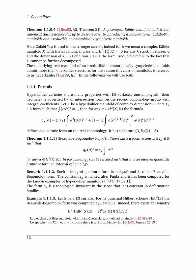
Theorem 1.1.0.4 ( [Bea83, §2, Théorèm 2]). Any compact Kähler manifold with trivialcanonical class is isomorphic up to an étale cover to a product of a complex torus, Calabi-Yaumanifolds and irreducible holomorphically symplectic manifolds.
Here Calabi-Yau is used in the stronger sense2, indeed for it we mean a complex Kählermanifold X with trivial canonical class and H0(⌦k
X ,C) = 0 for any k strictly between 0and the dimension of X . In Definition 1.1.0.1 the term irreducible refers to the fact thatX cannot be further decomposed.The underlying real manifold of an irreducible holomorphically sympelctic manifoldsadmits more than one Kähler structure, for this reason this class of manifolds is referredto as hyperkähler [Huy99, §1]. In the following we will use both.
�.�.� PeriodsHyperkähler varieties share many properties with K3 surfaces, one among all: theirgeometry is governed by an intersection form on the second cohomology group withintegral coefficients. Let X be a hyperkähler manifold of complex dimension 2n and �Xa 2-form such that
R(��)n = 1, then for any ↵ 2 H2(X ,R) the formula
qX (↵) = (n/2)Z↵2(��)n�1 + (1� n)
Z↵(�)n�1(�)nZ↵(�)n(�)n�1
defines a quadratic form on the real cohomology. It has signature (3, b2(X )� 3).
Theorem 1.1.1.1 ((Beauville-Bogomolov-Fujiki)). There exists a positive constant cX 2 Rsuch that
qX (↵)n = cX
Z↵2n
for any ↵ 2 H2(X ,R). In particular, qX can be rescaled such that it is an integral quadraticprimitive form on integral cohomology.
Remark 1.1.1.2. Such a integral quadratic form is unique3 and is called Beauville-Bogomolov form. The constant cX is named after Fujiki and it has been computed forthe known examples of hyperkähler manifolds ( [O’G, Table 1]).The form qX is a topological invariant in the sense that it is constant in deformationfamilies.
Example 1.1.1.3. Let S be a K3 surface. For its punctual Hilbert scheme Hilbn(S) theBeauville-Bogomolov form was computed by Beauville. Indeed, there exists an isometry
H2(Hilbn(S),Z) = H2(S,Z)�Z[E/2]2Rather than a Kähler manifold with trivial Chern class, as defined originally in [CHSW85].3Except when b2(X ) = 6, in which case there is a sign ambiguity (cf. [GHJ03, Remark 23.15]).
12
1.1 Irreducible holomorphically symplectic manifold
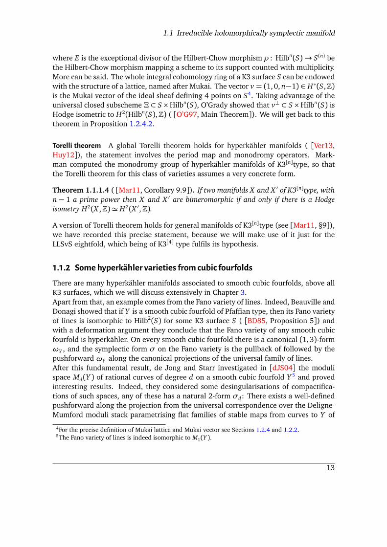
where E is the exceptional divisor of the Hilbert-Chow morphism ⇢ : Hilbn(S)! S(n) bethe Hilbert-Chow morphism mapping a scheme to its support counted with multiplicity.More can be said. The whole integral cohomology ring of a K3 surface S can be endowedwith the structure of a lattice, named after Mukai. The vector v = (1,0,n�1) 2 H⇤(S,Z)is the Mukai vector of the ideal sheaf defining 4 points on S4. Taking advantage of theuniversal closed subscheme ⌅ ⇢ S⇥Hilbn(S), O’Grady showed that v? ⇢ S⇥Hilbn(S) isHodge isometric to H2(Hilbn(S),Z) ( [O’G97, Main Theorem]). We will get back to thistheorem in Proposition 1.2.4.2.
Torelli theorem A global Torelli theorem holds for hyperkähler manifolds ( [Ver13,Huy12]), the statement involves the period map and monodromy operators. Mark-man computed the monodromy group of hyperkähler manifolds of K3[n]type, so thatthe Torelli theorem for this class of varieties assumes a very concrete form.
Theorem 1.1.1.4 ( [Mar11, Corollary 9.9]). If two manifolds X and X 0 of K3[n]type, withn � 1 a prime power then X and X 0 are bimeromorphic if and only if there is a Hodgeisometry H2(X ,Z)' H2(X 0,Z).
A version of Torelli theorem holds for general manifolds of K3[n]type (see [Mar11, §9]),we have recorded this precise statement, because we will make use of it just for theLLSvS eightfold, which being of K3[4] type fulfils its hypothesis.
�.�.� Somehyperkähler varieties from cubic fourfoldsThere are many hyperkähler manifolds associated to smooth cubic fourfolds, above allK3 surfaces, which we will discuss extensively in Chapter 3.Apart from that, an example comes from the Fano variety of lines. Indeed, Beauville andDonagi showed that if Y is a smooth cubic fourfold of Pfaffian type, then its Fano varietyof lines is isomorphic to Hilb2(S) for some K3 surface S ( [BD85, Proposition 5]) andwith a deformation argument they conclude that the Fano variety of any smooth cubicfourfold is hyperkähler. On every smooth cubic fourfold there is a canonical (1,3)-form!Y , and the symplectic form � on the Fano variety is the pullback of followed by thepushforward !Y along the canonical projections of the universal family of lines.After this fundamental result, de Jong and Starr investigated in [dJS04] the modulispace Md(Y ) of rational curves of degree d on a smooth cubic fourfold Y 5 and provedinteresting results. Indeed, they considered some desingularisations of compactifica-tions of such spaces, any of these has a natural 2-form �d: There exists a well-definedpushforward along the projection from the universal correspondence over the Deligne-Mumford moduli stack parametrising flat families of stable maps from curves to Y of
4For the precise definition of Mukai lattice and Mukai vector see Sections 1.2.4 and 1.2.2.5The Fano variety of lines is indeed isomorphic to M1(Y ).
13

1 Generalities
fixed genus and degree ( [dJS04, Corollary 4.3]). As before the pullback followed bythe pushforward along the projection of the universal family gives a 2-form on the stackthat in the end descends to the coarse moduli space ( [dJS04, § 3]). The form �d mayfail to be symplectic.In particular, �2 has generically rank 4, whereas dimM2(Y ) = 7; �3 has generically rank8 whereas dimM3(Y ) = 10. A natural problem is then understanding if there exists aMRC fibration of such spaces that admits a hyperkähler compactification.Given a general plane quadric Q on a cubic fourfold Y , the residual curve to Q in thelinear span of Q intersected with Y has degree 1, hence it is a line. This gives a rationalmap M2(Y ) ! F which is fibred in P3. So we have no new example of hyperkählervarieties.In the beautiful work [LLSvS17] the authors show that the compactfication of twistedcubics in the Hilbert scheme Hilb3t+1(Y ) admits a contraction to a hyperkähler manifoldof dimension 8 of K3[4] type. Its geometry is the subject of the present thesis.The variety of rational quartics has been studied in [Pet18]; for quintics we point therecent result in [LPZ20].
�.� Fourier-Mukai functorsFourier-Mukai functors are the most common operations intervening in the derivedworld of varieties, here we present the basics following quite closely [Huy06a] for thispresentation, which we nevertheless point to for a more thorough treatment.For a smooth projective variety X we denote by Db(X ) the bounded derived category ofcoherent sheaves. Let X and Y be smooth projective varieties, we denote the naturalprojections by
q : X ⇥ Y ! X p : X ⇥ Y ! Y.
Definition 1.2.0.1. 6 Given an object P 2 Db(X ⇥Y ), its associated Fourier-Mukai trans-form is
�P : Db(X )! Db(Y ), E 7! p⇤(P ⌦ q⇤E).The object P is called kernel of the Fourier-Mukai transform.
Fourier-Mukai functors enjoy many properties, the most important are: their composi-tion is again of Fourier-Mukai type, they admit both right and left adjoint functors. Letus see them.Let X1,X2 and X3 be smooth projective varieties andP 2 Db(X1⇥X2),Q 2 Db(X2⇥X3),then we define the convolution of the two kernels as
Q �P := ⇡12⇤�⇡⇤12P ⌦⇡
⇤23Q�.
6Fourier-Mukai functors were introduced by Mukai to prove that the derived categories of an abelianvariety and its dual are equivalent [Muk81]. The name Fourier is due to their resemblance with theconcept of Fourier transform for real vector spaces.
14
1.2 Fourier-Mukai functors
where ⇡i, j : X1 ⇥ X2 ⇥ X3! Xi ⇥ X j denote the natural projections
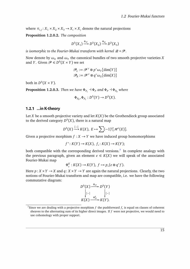
Proposition 1.2.0.2. The composition
Db(X1)�P�! Db(X2)
�Q�! Db(X3)
is isomorphic to the Fourier-Mukai transform with kernel Q �P .
Now denote by !X and !Y the canonical bundles of two smooth projective varieties Xand Y . Given P 2 Db(X ⇥ Y ) we set
PL :=P _ ⌦ p⇤!Y [dim(Y )]PR :=P _ ⌦ q⇤!X [dim(X )]
both in Db(X ⇥ Y ).
Proposition 1.2.0.3. Then we have �PL a �P and �P a �PR where
�PR ,�PL : Db(Y )! Db(X ).
�.�.� ...in K-theoryLet X be a smooth projective variety and let K(X ) be the Grothendieck group associatedto the derived category Db(X ), there is a natural map
Db(X )[�]�! K(X ), E 7!
X(�1)i[H i(E)].
Given a projective morphism f : X ! Y we have induced group homomorphisms
f ⇤ : K(Y )! K(X ), f⇤ : K(X )! K(Y );
both compatible with the corresponding derived versions.7 In complete analogy withthe previous paragraph, given an element e 2 K(X ) we will speak of the associatedFourier-Mukai map
�Ke : K(X )! K(Y ), f 7! p⇤(e⌦ q⇤ f ).
Here p : X ⇥Y ! X and q : X ⇥Y ! Y are again the natural projections. Clearly, the twonotions of Fourier-Mukai transform and map are compatible, i.e. we have the followingcommutative diagram:
Db(X )
[�]✏✏
�P// Db(Y )
[�]✏✏
K(X )�KP
// K(Y ).
7Since we are dealing with a projective morphism f the pushforward f⇤ is equal on classes of coherentsheaves to the alternating sum of its higher direct images. If f were not projective, we would need touse cohomology with proper support.
15
1 Generalities
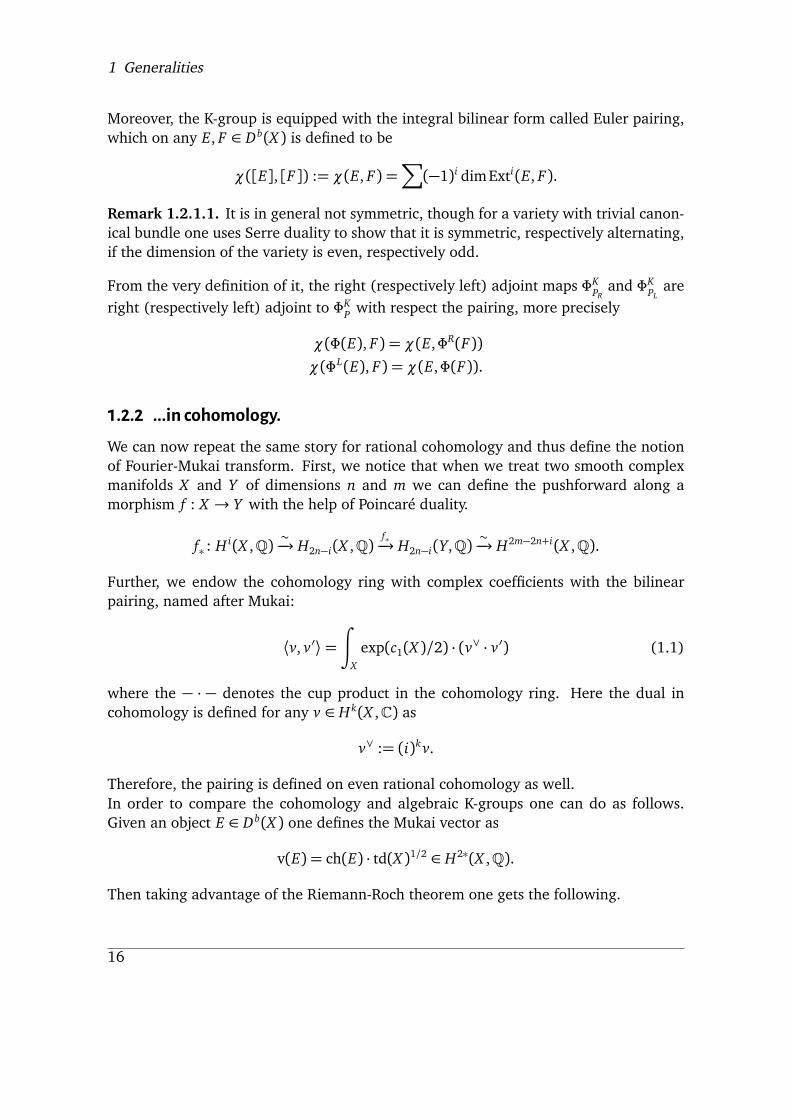
Moreover, the K-group is equipped with the integral bilinear form called Euler pairing,which on any E, F 2 Db(X ) is defined to be
�([E], [F]) := �(E, F) =X
(�1)i dimExti(E, F).
Remark 1.2.1.1. It is in general not symmetric, though for a variety with trivial canon-ical bundle one uses Serre duality to show that it is symmetric, respectively alternating,if the dimension of the variety is even, respectively odd.
From the very definition of it, the right (respectively left) adjoint maps �KPRand �K
PLare
right (respectively left) adjoint to �KP with respect the pairing, more precisely
�(�(E), F) = �(E,�R(F))�(�L(E), F) = �(E,�(F)).
�.�.� ...in cohomology.We can now repeat the same story for rational cohomology and thus define the notionof Fourier-Mukai transform. First, we notice that when we treat two smooth complexmanifolds X and Y of dimensions n and m we can define the pushforward along amorphism f : X ! Y with the help of Poincaré duality.
f⇤ : Hi(X ,Q) ⇠�! H2n�i(X ,Q)
f⇤�! H2n�i(Y,Q)⇠�! H2m�2n+i(X ,Q).
Further, we endow the cohomology ring with complex coefficients with the bilinearpairing, named after Mukai:
hv, v0i=Z
X
exp(c1(X )/2) · (v_ · v0) (1.1)
where the � · � denotes the cup product in the cohomology ring. Here the dual incohomology is defined for any v 2 Hk(X ,C) as
v_ := (i)kv.
Therefore, the pairing is defined on even rational cohomology as well.In order to compare the cohomology and algebraic K-groups one can do as follows.Given an object E 2 Db(X ) one defines the Mukai vector as
v(E) = ch(E) · td(X )1/2 2 H2⇤(X ,Q).
Then taking advantage of the Riemann-Roch theorem one gets the following.
16

1.2 Fourier-Mukai functors
Proposition 1.2.2.1 ( [Huy06a, Corollary 5.29]). The construction of Fourier-Mukaitransforms in cohomology and K–theory are compatible, that is for smooth projective vari-eties X and Y and an object P 2 Db(X ⇥ Y ) the diagram
K(X )
v✏✏
�KP// K(Y )
v✏✏
H⇤(X ,Q) �HP// H⇤(Y,Q).
(1.2)
is commutative. Moreover, the Mukai vector respects the pairing on the two groups, i.e. forany object E, F 2 Db(X ⇥ Y )
�([E], [F]) = hv(E), v(F)i.
It is good to point out that in general the integral structure of K–groups and cohomologygroups may behave very differently. Although the image of the Mukai pairing may bevery small, we have though this surprising result.
Proposition 1.2.2.2 ( [Huy06a, Proposition 5.44]). If the Fourier-Mukai functor �P :Db(X )! Db(Y ) is an equivalence, then �H
P is an isometry on the whole rational cohomol-ogy rings.
�.�.� Topological K-theoryWe now turn to topological K-theory. In the end for the spaces we are interested in(namely K3 surfaces and smooth cubic fourfolds) their topological K-group coincideswith the Grothendieck ring of topological C-vector bundles, which is isomorphic via theMukai vector to the integral cohomology ring. Here we give a brief account, referencesare [AH62], [AH59] and [AH61].For a smooth variety X we set:
Ktop(X ) = K0(X )� K1(X ).
where K1(X ) is the kernel of the homomorphism K0(X ⇥ S1)! K0(X ) induced from theembedding X ! X ⇥ S1. Making use of the Bott periodicity theorem, Ktop(X ) is turnedin a graded anti-commutative ring [AH61, Proposition page 203]. The analytificationof sheaves on X induces a natural morphism From algebraic K-theory to topologicalK-theory
K(X )! Ktop(X ).
A mapch : Ktop(X )! H⇤(X ,Q)
is constructed. It extends the usual Chern character from the Grothendieck group andit is called Chern character, too. It has the following properties:
17
1 Generalities
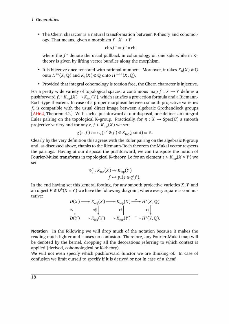
• The Chern character is a natural transformation between K-theory and cohomol-ogy. That means, given a morphism f : X ! Y
ch� f ⇤ = f ⇤ � ch
where the f ⇤ denote the usual pullback in cohomology on one side while in K–theory is given by lifting vector bundles along the morphism.
• It is bijective once tensored with rational numbers. Moreover, it takes K0(X )⌦Qonto H2⇤(X ,Q) and K1(X )⌦Q onto H2⇤+1(X ,Q).
• Provided that integral cohomology is torsion free, the Chern character is injective.
For a pretty wide variety of topological spaces, a continuous map f : X ! Y defines apushforward f⇤ : Ktop(X )! Ktop(Y ), which satisfies a projection formula and a Riemann-Roch-type theorem. In case of a proper morphism between smooth projective varietiesf⇤ is compatible with the usual direct image between algebraic Grothendieck groups[AH62, Theorem 4.2]. With such a pushforward at our disposal, one defines an integralEuler pairing on the topological K–group. Practically, for ⇡ : X ! Spec(C) a smoothprojective variety and for any e, f 2 Ktop(X ) we set:
�(e, f ) := ⇡⇤(e_ ⌦ f ) 2 Ktop(point)' Z.Clearly by the very definition this agrees with the Euler pairing on the algebraic K-groupand, as discussed above, thanks to the Riemann-Roch theorem the Mukai vector respectsthe pairings. Having at our disposal the pushforward, we can transpose the notion ofFourier-Mukai transforms in topological K–theory, i.e for an element e 2 Ktop(X ⇥ Y ) weset
�Ke : Ktop(X )! Ktop(Y )
f 7! p⇤(e⌦ q⇤ f ).
In the end having set this general footing, for any smooth projective varieties X ,Y andan object P 2 Db(X ⇥Y ) we have the following diagram, where every square is commu-tative:
D(X )
�P
✏✏
// Kalg(X )
�KP✏✏
// Ktop(X )
�KP✏✏
v// H⇤(X ,Q)�HP
✏✏
D(Y ) // Kalg(Y ) // Ktop(Y )v
// H⇤(Y,Q).
Notation In the following we will drop much of the notation because it makes thereading much lighter and causes no confusion. Therefore, any Fourier-Mukai map willbe denoted by the kernel, dropping all the decorations referring to which context isapplied (derived, cohomological or K–theory).We will not even specify which pushforward functor we are thinking of. In case ofconfusion we limit ourself to specify if it is derived or not in case of a sheaf.
18

1.2 Fourier-Mukai functors
�.�.� O’Grady result revisited.
K-theoryofK� surfaces Let S be a K3 surface, then by explicit computation one gets thatthe Mukai vector for an object E 2 Db(S) is integral. First one computes the Todd class
td(S) = (1,0,2)
and then
v(E) = ch(E) ·∆
td(S) =�rk(E), c1(E), rk(E) + c21(E)/2� c2(E)
�.
Since the intersection form on H2(S,Z) is even, it is indeed an integral vector. The sameholds for a complex vector bundle on S and we have
Proposition 1.2.4.1. Let S be a K3 surface, then the Mukai vector
v: Ktop(S)! H⇤(S,Q)
factors through an isometry on the integral cohomology.
Proof. We have seen that the Mukai vector for a K3 surface S is integral. Since theintegral cohomology of S is torsion free, it is injective by [AT14, Theorem 2.1, (1)] and,using [AT14, Theorem 2.1, (3)], one easily shows that it is surjective.
Moreover, since the canonical bundle on S is trivial, the Mukai pairing is symmetric oneven cohomology and therefore on the whole cohomology. The pairing can be explicitlyso written
h(v1, v2, v3), (w1,w2,w3)i= vow4 + v1w1 + v4w0
for any (v0, v2, v4), (w0,w2,w4) 2 H⇤(S,Z).One endows H⇤(S,Z) with a Hodge structure by retaining the one on H2(S,Z) and byimposing H0(S,Z) � H4(S,Z) to be of weight two. Via the Mukai vector one endowsKtop with an integral Hodge structure as well.
O’Grady result revisited. We rewrite [O’G97, Main Theorem] in terms of the setting wehave introduced.
Proposition 1.2.4.2. Let S be a K3 surface and S[n] be its Hilbert scheme of n points, thenthe composition
[I⇠]? ⇢ Ktop(S)I_⌅�! Ktop(S[n])
c1�! H2(S[n],Z) (1.3)
where I⇠ is the ideal sheaf of four points in S, is a Hodge isometry.
19

1 Generalities
Proof. We consider the map (1.3). By the above discussion on K3 surfaces passing tocohomology is harmless, indeed the Mukai vector takes the class of I⇠ to v = v(I⇠) =(1,0,n� 1) and takes [I⇠]? isometrically to v?. We are then left to prove that
v? ,! H⇤(S,Z)I_⌅�! H⇤(S[n],Q) c1�! H2(S[n],Z). (1.4)
is an isometry. For every k 2 v? we compute
k 7! c1�p⇤�v(I_⌅) · q
⇤k��
=
c1�p⇤�ch(I⌅)_ · p⇤ td(S[n])1/2 · q⇤ td(S)1/2 · q⇤k
��=
c1�td(S[n])1/2 · p⇤�ch(I⌅)_ · q⇤ td(S)1/2 · q⇤k
�� (1.5)
where the last equality holds because of projection formula. The Todd class of a K3surface was discussed above, its root is the sum of 1 and the fundamental class of thesurface. Since S[n] is hyperkähler, its first Chern class is trivial as well as its canonicalbundle and its Todd class does not contribute to the last quantity. Finally, S[n] being afine moduli space 8, the similitude of I⌅ is 19 (in other words its rank is one) and thus,after the computation (1.5), the map in (1.4) coincides with the O’Grady map, which isknown to be an isometry [O’G97, Main Theorem].
�.� Kuznetsov component and itsMukai latticeThe world of cubic fourfolds and K3 surfaces are deeply intertwined: Hassett inves-tigated it from a Hodge theoretic view point. More recently Kuznetsov studied theirderived categories and thanks to Addington and Thomas now we can compare the twoperspectives. In this section we want to introduce the Kuznetsov component of thederived category of cubic fourfolds (see Theorem 1.3.1.7) and its Mukai lattice in topo-logical K-theory (see Definition 1.3.2.1).
�.�.� Kuznetsov componentLet T be a triangulated category and i : B ⇢ T a subtriangulated category. For sim-plicity we will restrict to categories that are C–linear and with finite dimensional Homvector spaces.8Here, we should more correctly say that S[n] is isomorphic to the moduli space of semistable sheaveswith fixed Mukai vector (1,0,n�1), the isomorphism being given by mapping a subscheme of lengthn to its ideal sheaves. For an accurate proof of such statement we point to [KPS18, Lemma B.5.6].
9If M is a moduli space of semistable sheaves with Hilbert polynomial P on S, a quasi-universal familyof semistable sheaves F 2 Coh(S⇥M) is called quasi-universal of similitude ⇢ if for any T -flat familyE 2 Coh(S⇥ T ) of semistable sheaves with Hilbert polynomial P there exists a locally free OT -moduleV of rank ⇢ such that E ⌦ p⇤V = �⇤F , where p : S ⇥ T ! T is the projection and � : T ! M is theclassifying morphism.
20

1.3 Kuznetsov component and its Mukai lattice
Definition 1.3.1.1. The categoryB is said to be right admissible if the following equivalentconditions are satisfied:
(i) The inclusion functor i admits a right adjoint funtor i a R.
(ii) For every element T 2 T there exists an exact triangle
B! T ! C ! B[1]
where B is in an element inB and C is such that HomT (B1,C) = 0 for every objectB1 2B .
Specularly one can define the notion of left admissible for a subtriangulated category. If cBis both right and left admissible, then it is called admissible.
To see the equivalence: For the direct implication, one uses the counit morphism andcomplete it to a triangle to get the exact triangle
iR(X ) =: Bcounit���! T ! C ! B[1].
Invoking the faithfulness of Yoneda functor one checks that C satisfies the wanted con-dition. Conversely, taking advantage of the condition on the Hom sets, one shows thatthe triangle in condition (ii) is unique, the association T 7! B is well-defined and givesrise to a functor R : T ! B . Applying Hom(B1,�) to the triangle, one gets that R isright adjoint.The two notions of left and right admissible subtriangulated category are strictly boundedtogether. Indeed, if we set
B? = {T 2 T : HomT (B, T ) = 0, 8B 2B}?B = {T 2 T : HomT (T,B) = 0, 8B 2B}
Applying the same ideas above, it is easy to check that C :=B? is left admissible andthat ?(B?) =B . In the end, we have thatB andC are two subtriangulated categoriesthat generate T and each is orthogonal (with direction) to the other. We then come tothe following more general
Definition 1.3.1.2. Given a triangulated category T , a semi-orthogonal decomposition
T = hT1, ...,Tni
of T consists of a sequence of full subtriangulated categories T1, ...,Tn such that
• Hom(Ti,T j) = 0 for every i > j.
21
1 Generalities
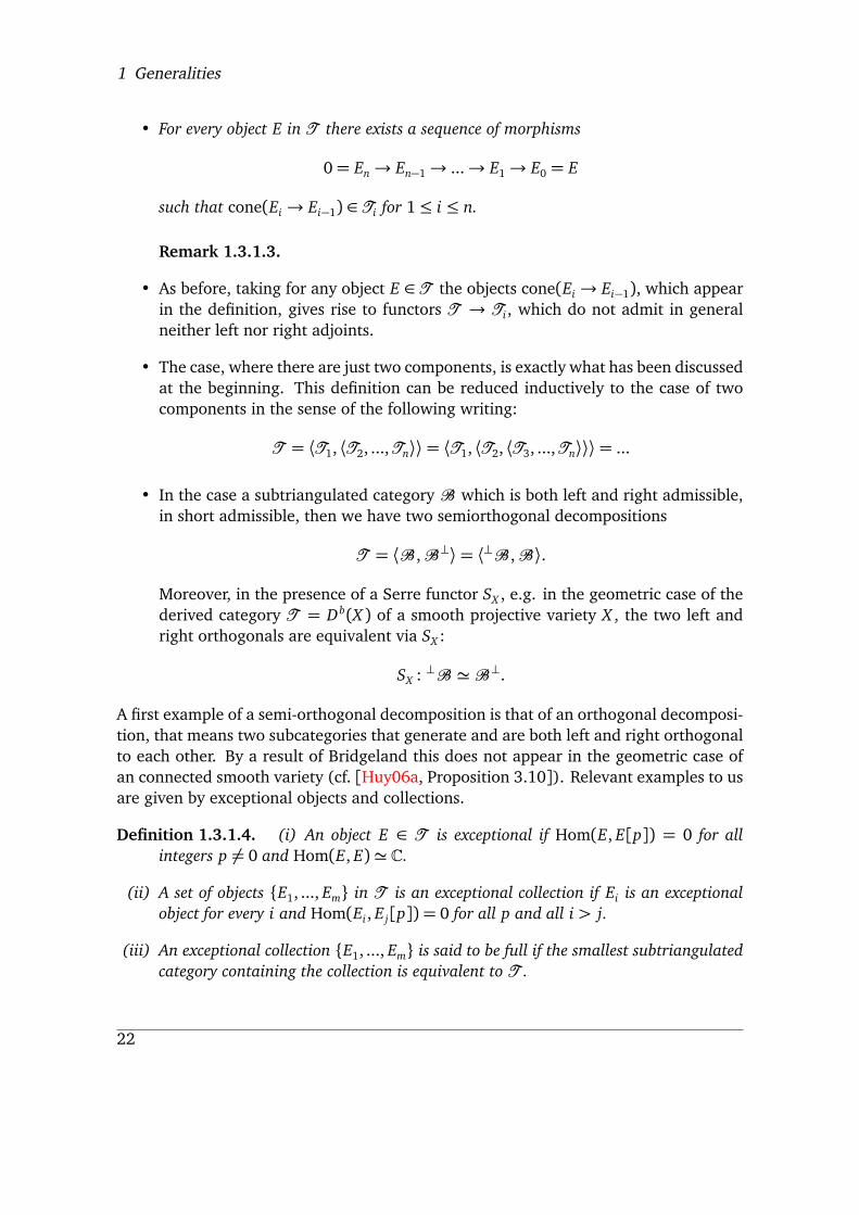
• For every object E in T there exists a sequence of morphisms
0= En! En�1! ...! E1! E0 = E
such that cone(Ei ! Ei�1) 2 Ti for 1 i n.
Remark 1.3.1.3.
• As before, taking for any object E 2 T the objects cone(Ei ! Ei�1), which appearin the definition, gives rise to functors T ! Ti, which do not admit in generalneither left nor right adjoints.
• The case, where there are just two components, is exactly what has been discussedat the beginning. This definition can be reduced inductively to the case of twocomponents in the sense of the following writing:
T = hT1, hT2, ...,Tnii= hT1, hT2, hT3, ...,Tniii= ...
• In the case a subtriangulated categoryB which is both left and right admissible,in short admissible, then we have two semiorthogonal decompositions
T = hB ,B?i= h?B ,Bi.
Moreover, in the presence of a Serre functor SX , e.g. in the geometric case of thederived category T = Db(X ) of a smooth projective variety X , the two left andright orthogonals are equivalent via SX :
SX :?B 'B?.
A first example of a semi-orthogonal decomposition is that of an orthogonal decomposi-tion, that means two subcategories that generate and are both left and right orthogonalto each other. By a result of Bridgeland this does not appear in the geometric case ofan connected smooth variety (cf. [Huy06a, Proposition 3.10]). Relevant examples to usare given by exceptional objects and collections.
Definition 1.3.1.4. (i) An object E 2 T is exceptional if Hom(E, E[p]) = 0 for allintegers p 6= 0 and Hom(E, E)' C.
(ii) A set of objects {E1, ..., Em} in T is an exceptional collection if Ei is an exceptionalobject for every i and Hom(Ei, Ej[p]) = 0 for all p and all i > j.
(iii) An exceptional collection {E1, ..., Em} is said to be full if the smallest subtriangulatedcategory containing the collection is equivalent to T .
22

1.3 Kuznetsov component and its Mukai lattice
The smallest subtriangulated category hEi containing an exceptional object E is admis-sible. Indeed, the right and left adjoints to the inclusion are given by
F 7! Hom•(E, F)⌦ EF 7! Hom•(F, E)⇤ ⌦ E
Here, it is fundamental to assume that the category has finite dimensional Hom (vectorspaces). Exceptional objects define admissible subcategories, therefore from exceptionalcollections we get semi-orthogonal decompositions
T = hA , E1, ..., Emi= hE1, ..., Em,Bi
where A = E?1 \ ... \ E?m and B = ?E1 \ ... \ ?Em. Notice that A and B are ab-stractly equivalent but differently embedded. In this case, to pass from one descriptionto another it is rather easy.
Definition 1.3.1.5. Let E be an exceptional object. The functors
LE : F 7! cone(Hom(E, F)⌦ E! F)RE : F 7! cone(F_ ! Hom(E, F)_ ⌦ E_)
are called left and right mutation past E.
These functors have this special property (e.g. [Kuz09, Theorem 2.9,2.10]): If T =hE1, ..., Emi is an orthogonal decomposition given by a collection of exceptional objects,then
T = hE1, ...Ei�1,LEi Ei+1, Ei, Ei+2, .., Emi
is a semi-orthogonal decomposition as well. Similarly, using the right mutating functor,we get the semi-orthogonal decomposition
T = hE1, ...Ei�1, Ei,REi Ei�1, Ei+2, .., Emi.
As an example to illustrate the theory introduced so far we present the classical resultfrom Beilinson: the semiorthogonal decomposition of Db(Pn).
Example 1.3.1.6 ( [Huy06a, Corollary 8.29] ). The derived category of Pn admits thesemiorthogonal decomposition
Db(Pn) = hOPn(�n), ...,OPni.
From the line
Hom•(OPn(i),OPn( j)) = H•(Pn,OPn( j � i)) =ß C i f i = j,
0 i f � n j � i < 0
23

1 Generalities
we see that it is an exceptional collection. Using the Beilinson resolution of the diagonal� in Pn ⇥ Pn
0!^n(O (�1)Ç⌦(1))!^n�1(O (�1)Ç⌦(1))! ...!OPn⇥Pn !O�! 0
one proves the fullness of the sequence, that is the sequence generates the whole cate-gory Db(Pn) (cf. [Huy06a, Corollary 8.29]).Once this decomposition is proven, one mutates OPn(�n) right past through the othersheaves and finds another decomposition
Db(Pn) = hOPn(�n+ 1), ...,OPn ,R�n+1R�n+2...R1OPn(�n+ 1)i
The object R�n+1R�n+2...R1OPn(�n+ 1) is now equal to OPn(1), because it is orthogonalto OPn(k) for every k = �n+ 1, .., 0 (cf. Remark 1.3.1.3). So we get that for i = 1
Db(Pn) = hOPn(�n+ i), ...,OPn(i)i .
is a semiorthogonal decomposition as well. Iteratingwe prove that these are semiorthog-onal decompositions for any i 2 Z. So we get the claimed decomposition for i = 1,iterating we get the others, too.
Let X be a smooth projective Fano variety of index k, that is the canonical bundle KX isanti-ample and �KX = OX (k), where OX (1) denotes the restriction of the polarisation.Relying on Beilinson’s result (cf. Example 1.3.1.6) one proves OX , ...,OX (k � 1) is anexceptional collection. Because of Serre duality we cannot go further with OX (k) (inthe sense that OX , ...,OX (k � 1) is not exceptional), nevertheless the collection may notgenerate, in contrast with the example of Pn above. It becomes therefore of interest tostudy the orthogonal complement of the exceptional collection. This has been done ingreat generality, in the case of cubic fourfolds (which are Fano of index 4) we have thefollowing result by Kuznetsov.
Theorem 1.3.1.7 ( [Kuz10]). Let Y be a smooth cubic fourfold then
A := hOY ,OY (1),OY (2)i?
is a non-commutative K3 surface, that means thatA is indecomposable, with Serre functorgiven by the shift by 2 and with Hochschild cohomology and homology of a K3 surface.
The categoryA is known as Kuznetsov component. In general, it is not knownwhen it isequivalent to the derived category of an honest K3 surface: According to the Kuznetsovconjecture ( [Kuz10, Conjecture 1.1]) it is so, when Y is rational (see [HLS19, § 3] fora more comprehensive treatise).
24

1.3 Kuznetsov component and its Mukai lattice
Remark 1.3.1.8. There is nothing special about the sequence OY ,OY (1),OY (2), indeedone could have chosen another sequence, too. Tensoring with OY (�1) give rises to anautoequivalence of Db(Y ) and we get a new semi-orthogonal decomposition
D(Y ) = hA 0,OY (�1),OY ,OY (1)i.
Applying the right mutation ROY (�1) we get
D(Y ) = hOY (�1),ROY (�1)(A 0),OY ,OY (1)i= hROY (�1)(A 0),OY ,OY (1),OY (2)i.In the end we have an autoequivalence
A⌦O (�1)����!A 0
ROY (1�)����!A .
�.�.� Topological K–theory of theKuznetsov componentAddington and Thomas introduced a Mukai lattice for the Kuznetsov component andstudied their properties taking advantage of the topological K–theory of cubic fourfolds.We introduce here the definitions and postpone to Chapter 3 the arithmetic properties.Anything herein comes from [AT14].Let Y be a smooth cubic fourfold and letA be the associated Kuznetsov component.
Definition 1.3.2.1. The Mukai lattice ofA is
Ktop(A ) = {k 2 Ktop(Y ): �(OY (i), k) = 0 for i = 0,1,2}.
It is endowed by a Hodge structure by pulling-back the one of weight zero on the totalcohomology of the cubic fourfold
H⇤(Y,Z) =M
i
H2i(Y,Z)(i)
along the Chern character.
In other words, the group underlying Ktop(A ) is the right orthogonal complement to thegroup generated by the classes of OY ,OY (1),OY (2). Thus, we have a natural projectionpr: Ktop(Y )! Ktop(A ). The Euler pairing endows Ktop(A )with the structure of a lattice( [Huy18, Proposition 1.20]). We set
�1 := pr[Oline(1)] �2 := pr[Oline(2)]
where pr: Ktop(Y ) ! Ktop(A ) is the orthogonal projection. The two elements gener-ate a primitive sublattice which is isomorphic to A2 (e.g. [Huy18, Lemma 1.18]), theorthogonal complement is the primitive cohomology.
Proposition 1.3.2.2 ( [AT14, Thm 6]). The Mukai vector v: Ktop(Y ) ! H⇤(Y,Q) takesh�1,�2i? ⇢ Ktop(A ) isometrically onto H4
prim(Y,Z).We will come back to other properties of the Mukai lattice in Chapter 4, where we willspend some words on the arithmetic properties of Ktop(A ).
25


�Theperiods of the Lehn–Lehn–Sorger–vanStraten variety
This chapter is devoted to compute the periods of the LLSvS variety, or better to relatethem to the periods of the associated cubic fourfold; this work appeared in our paper[AG20] in collaboration with Nicolas Addington.Periods are one of the most important invariants of hyperkähler manifolds, indeed theintegral Hodge structure on the second cohomology group governs most of the geometryof such manifolds as expressed in the Torelli theorem.Therefore, understanding the Hodge structure is of fundamental importance. Variousresults are known in this direction, of paramount importance for us will be the case ofthe Fano varieties of lines on a smooth cubic fourfold. Beauville and Donagi [BD85],after having proven that such a variety is hyperkähler, showed that the cubic fourfold Yand its Fano variety of lines F have the same periods, the isomorphism being given bythe correspondence of the universal family of lines.
Theorem 2.0.0.1 ( [BD85, Proposition 4]). Let Y be a smooth cubic fourfold, F be itsFano variety of lines and let L ⇢ F ⇥Y be the universal family of lines, with p : L! Y andq : L! F the natural projections. Then
q⇤p⇤ : H4
prim(Y,Z)! H2prim(F,Z) (2.1)
is an isometry.
Our result relates the cohomology of the cubic fourfold with the associated LLSvS variety.We begin with the following statement regarding the primitive cohomology.Let Y be a smooth cubic fourfold not containing a plane. We consider the contraction
u: M ! Z
from the ten-dimensional space of generalized twisted cubics on Y to the LLSvS sym-plectic eightfold (see [LLSvS17, Theorem B]). Let C ⇢ Y ⇥M be the universal curve.
Theorem 2.0.0.2 ( [AG20, Theorem 1]). The pullback
u⇤ : H2(Z ,Z)! H2(M ,Z)
27

2 The periods of the Lehn–Lehn–Sorger–van Straten variety
is injective, and the map[C]⇤ : H4(Y,Z)! H2(M ,Z) (2.2)
restricts to a Hodge isometry
[C]⇤ : H4prim(Y,Z)
⇠�! u⇤(H2
prim(Z ,Z)), (2.3)
with the intersection pairing on the left-hand side and the opposite of the Beauville–Bogomolov–Fujiki pairing on the right.
For a statement about the full H2(Z ,Z), we must recall Kuznetsov’s K3 category
A = hOY ,OY (h),OY (2h)i? ⇢ Db(Y ),
the Mukai lattice introduced in [AT14, §2],
Ktop(A ) = {[OY ], [OY (h)], [OY (2h)]}? ⇢ Ktop(Y ),
and the two special classes �1,�2 2 Ktop(A ), which we discussed in Section 1.3.2.
Theorem 2.0.0.3 ( [AG20, Theorem 1]). We retain the notation of Theorem 2.0.0.2. Let
�K : Ktop(A ) ⇢ Ktop(Y )! Ktop(M)
be the map on topological K-theory induced by the Fourier–Mukai kernel I_C (�3h) 2 Db(Y⇥M). Then the map
c1 ��K : Ktop(A )! H2(M ,Z) (2.4)
restricts to a Hodge isometry
h�2 ��1i?⇠�! u⇤(H2(Z ,Z)), (2.5)
with the Euler pairing on the left-hand side and the opposite of the Beauville–Bogomolov–Fujiki pairing on the right.
One of the main ideas of [AL17] is that Z is a moduli space of complexes inA containingthe projections of Oy for points y 2 Y ; the K-theory class of these complexes is �2 ��1,so (2.5) is natural in light of O’Grady’s description of the period of a moduli spaceof sheaves on a K3 surface [O’G97, Main Theorem]. Li, Pertusi, and Zhao developedthis idea further using Bridgeland stability conditions in [LPZ18]; note that their class2�1 + �2 is related to our �2 � �1 by an autoequivalence of A (e.g. [Huy17a, Proposi-tion 3.12]). Statements similar to Theorem 2.0.0.3 appear in [LPZ18, Proposition 5.2]and [BLM+19, Theorem 29.2(2)]. We believe nonetheless that our approach is of itsown interest as our proofs require less machinery, the statement in Theorem 2.0.0.2 isvery classical and explicit.1
1After the first version of the paper [AG20] was posted, Li, Pertusi, and Zhao informed us that thesubmitted version of [LPZ18] includes a statement analogous to our Theorem 3(c).
28
2.1 A first approach to the periods of LLSvS variety
�.� Afirst approach to the periods of LLSvS varietyHere we propose a first naive approach to relate the periods of the LLSvS variety to theones of the cubic fourfolds. This is instructive and will elaborate on this in the nextsections, where we get the main result.The first idea was to look at the correspondence given by the universal curve C ⇢ Y ⇥M ,although it looks very difficult to descend the action on Z , because there is no family ofcurves on Z that could do the work. Moreover, the family C per se is not smooth, thusit is better to look at the action by cup product of its cohomology class [C] and at thecomposition in cohomology with rational coefficients:
H4(Y,Q)pr⇤Y�! H4(Y ⇥M 0,Q) �[[C]���! H10(Y ⇥M 0,Q) prM⇤��! H2(M ,Q).
This is a natural generalisation of the correspondence used by Beauville and Donagi,because being the universal family of lines L ⇢ Y ⇥ F smooth, the morphism (2.1)equals
H4(Y,Q)pr⇤Y�! H4(Y ⇥ F,Q) �[[L]���! H8(Y ⇥ F,Q) prF⇤��! H2(F,Q).
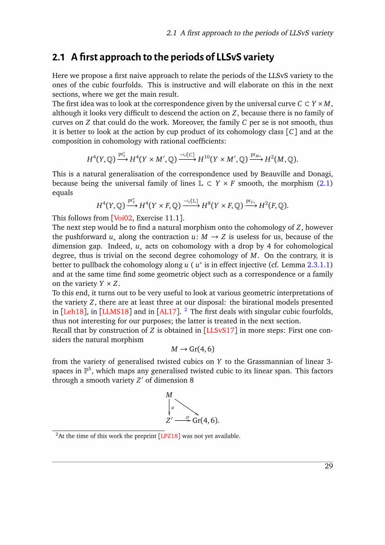
This follows from [Voi02, Exercise 11.1].The next step would be to find a natural morphism onto the cohomology of Z , howeverthe pushforward u⇤ along the contraction u: M ! Z is useless for us, because of thedimension gap. Indeed, u⇤ acts on cohomology with a drop by 4 for cohomologicaldegree, thus is trivial on the second degree cohomology of M . On the contrary, it isbetter to pullback the cohomology along u ( u⇤ is in effect injective (cf. Lemma 2.3.1.1)and at the same time find some geometric object such as a correspondence or a familyon the variety Y ⇥ Z .To this end, it turns out to be very useful to look at various geometric interpretations ofthe variety Z , there are at least three at our disposal: the birational models presentedin [Leh18], in [LLMS18] and in [AL17]. 2 The first deals with singular cubic fourfolds,thus not interesting for our purposes; the latter is treated in the next section.Recall that by construction of Z is obtained in [LLSvS17] in more steps: First one con-siders the natural morphism
M ! Gr(4,6)
from the variety of generalised twisted cubics on Y to the Grassmannian of linear 3-spaces in P5, which maps any generalised twisted cubic to its linear span. This factorsthrough a smooth variety Z 0 of dimension 8
Ma
✏✏
$$
Z 0 �// Gr(4,6).
2At the time of this work the preprint [LPZ18] was not yet available.
29
2 The periods of the Lehn–Lehn–Sorger–van Straten variety
The variety Z is obtained from a (divisorial) further contraction b : Z 0 ! Z . We denoteby u the composition M ! Z 0 ! Z .The strategy adopted in this section is based on the result of Lahoz, Lehn, Macrì and Stel-lari, who describe the variety Z 0 as a moduli space of Gieseker stable sheaves (We werenot able to take advantage of their major result about Z (cf. [LLMS18, Theorem B])!).Having this at our disposal we will cook up a correspondence � : H4(Y.Z)! H2(Z 0,Z)to get the following Theorem 2.1.0.1.Let us define �. Let U be the quasi-universal family on Y ⇥Z 0 and let ⇢ be its similitude.The Grassmaniann Gr := Gr(4,V ) parametrises a family of cubic surfaces on Y givenby intersecting each E 2 Gr with Y , we call S the pullback of this family along themorphism � : Z 0 ! Gr. We define
F := ch3(OS )�ch3(U)⇢(U)
2 H6(Y ⇥ Z 0,Q)
and call � the composition in cohomology with rational coefficients
H4(Y,Q)pr⇤Y�! H4(Y ⇥ Z 0,Q) �[F��! H10(Y ⇥ Z 0,Q) prZ0⇤��! H2(Z 0,Q).
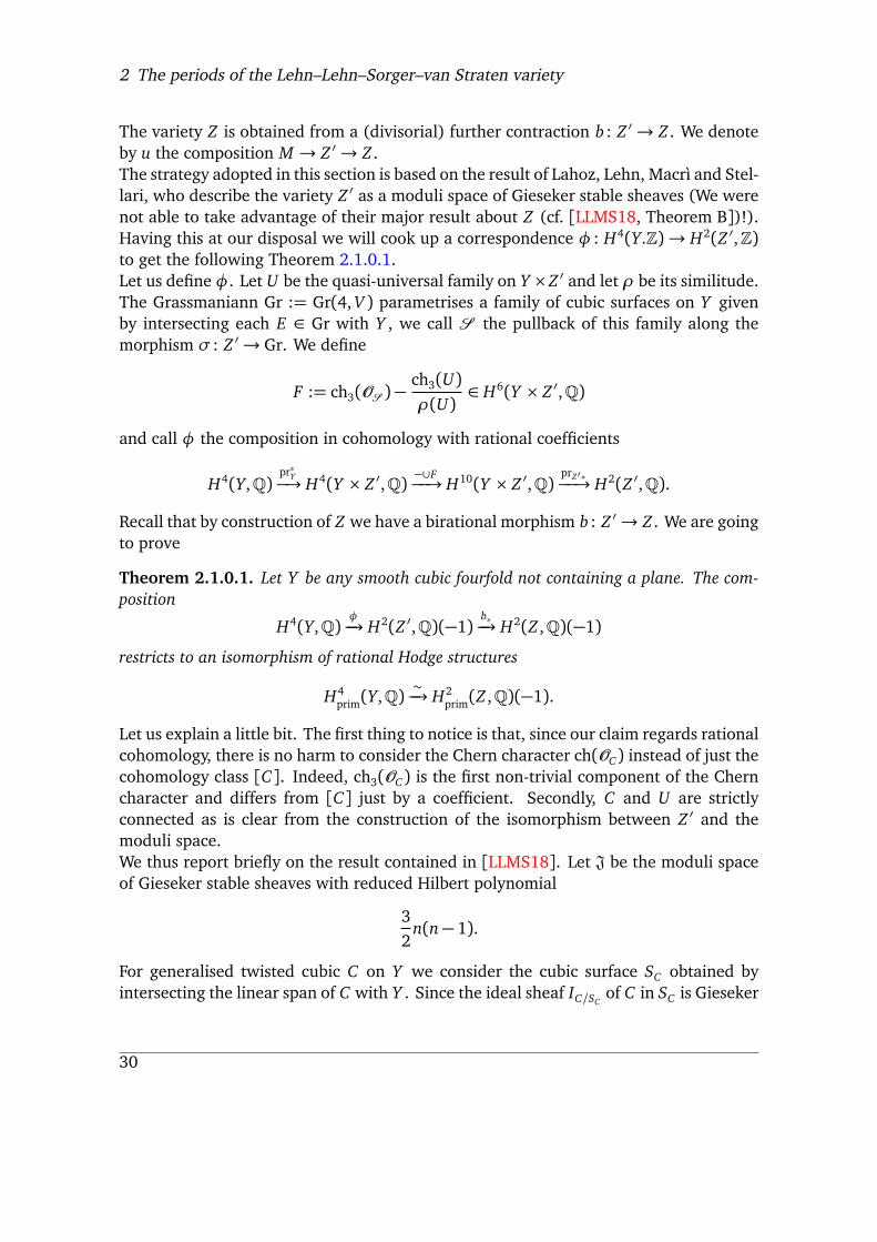
Recall that by construction of Z we have a birational morphism b : Z 0 ! Z . We are goingto prove
Theorem 2.1.0.1. Let Y be any smooth cubic fourfold not containing a plane. The com-position
H4(Y,Q) ��! H2(Z 0,Q)(�1) b⇤�! H2(Z ,Q)(�1)restricts to an isomorphism of rational Hodge structures
H4prim(Y,Q)
⇠�! H2
prim(Z ,Q)(�1).
Let us explain a little bit. The first thing to notice is that, since our claim regards rationalcohomology, there is no harm to consider the Chern character ch(OC) instead of just thecohomology class [C]. Indeed, ch3(OC) is the first non-trivial component of the Cherncharacter and differs from [C] just by a coefficient. Secondly, C and U are strictlyconnected as is clear from the construction of the isomorphism between Z 0 and themoduli space.We thus report briefly on the result contained in [LLMS18]. Let J be the moduli spaceof Gieseker stable sheaves with reduced Hilbert polynomial
32n(n� 1).
For generalised twisted cubic C on Y we consider the cubic surface SC obtained byintersecting the linear span of C with Y . Since the ideal sheaf IC/SC of C in SC is Gieseker
30
2.1 A first approach to the periods of LLSvS variety
stable for any twisted cubic C on Y ( [LLMS18, Lemma 1.1]), the idealI of the universalcurveC inside the familySM
3 of surfaces gives a morphism M ! J. This descends to anisomorphism Z 0 ! J1 on an irreducible component J1 ⇢ J ( [LLMS18, Propostion 1.2].Over the moduli space J we have a universal family of sheaves, let U be its restrictionon J. We compare the correspondence given by U on Y ⇥ Z 0 with the one given by theuniversal curve C in Y ⇥ M . By the discussion above and the universal property of Uwe have an isomorphism
a⇤U = IC/S ⌦ pr⇤M E (2.6)
for some vector bundle E on M .
Remark 2.1.0.2. By the short exact sequence
0!IC /S ! OS ! OC ! 0
and the additivity of the Chern character we have
ch(IC /S ) = ch(OS )� ch(OC ).
Moreover, by [Ful84, Example 15.3.1] we get
ch(IC /S ) = [S ] + (�6[C] + ch3(OS )) + higher-order terms. (2.7)
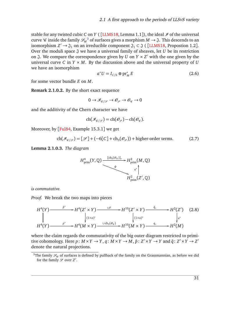
Lemma 2.1.0.3. The diagram
H4prim(Y,Q)
[ch3(OC )]⇤//
�
))
H2prim(M ,Q)
H2prim(Z
0,Q)a⇤
OO
is commutative.
Proof. We break the two maps into pieces
H4(Y )p⇤
// H4(Z 0 ⇥ Y ) [F//
(1⇥a)⇤✏✏
H10(Z 0 ⇥ Y )q⇤
//
(1⇥a)⇤✏✏
H2(Z 0)
a⇤✏✏
H4(Y )p⇤
// H4(M ⇥ Y )[ ch3(OC )
// H10(M ⇥ Y )q⇤
// H2(M)
(2.8)
where the claim regards the commutativity of the big outer diagram restricted to primi-tive cohomology. Here p : M⇥Y ! Y , q : M⇥Y ! M , p : Z 0⇥Y ! Y and q : Z 0⇥Y ! Z 0
denote the natural projections.3The family SM of surfaces is defined by pullback of the family on the Grassmannian, as before we didfor the family S over Z 0.
31
2 The periods of the Lehn–Lehn–Sorger–van Straten variety
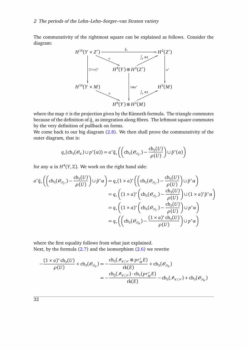
The commutativity of the rightmost square can be explained as follows. Consider thediagram:
H10(Y ⇥ Z 0)q⇤
//
(1⇥a)⇤
✏✏
⇡
((
H2(Z 0)
a⇤
✏✏
H8(Y )⌦ H2(Z 0)
1⌦a⇤
✏✏
RY ⌦1
77
H10(Y ⇥M)⇡
((
H2(M)
H8(Y )⌦ H2(M)
RY ⌦1
77
where the map⇡ is the projection given by the Künneth formula. The triangle commutesbecause of the definition of q⇤ as integration along fibres. The leftmost square commutesby the very definition of pullback on forms.We come back to our big diagram (2.8). We then shall prove the commutativity of theouter diagram, that is:
q⇤(ch3(OC )[ p⇤(↵)) = a⇤q⇤
ÅÅch3(OSZ0 )�
ch3(U)⇢(U)
ã[ p⇤(↵)ã
for any ↵ in H4(Y,Z). We work on the right hand side:
a⇤q⇤
ÅÅch3(OSZ0 )�
ch3(U)⇢(U)
ã[ p⇤↵ã= q⇤(1⇥ a)⇤ÅÅ
ch3(OSZ0 )�ch3(U)⇢(U)
ã[ p⇤↵ã
= q⇤
Å(1⇥ a)⇤Åch3(OSZ0 )�
ch3(U)⇢(U)
ã[ (1⇥ a)⇤ p⇤↵ã
= q⇤
Å(1⇥ a)⇤Åch3(OSZ0 )�
ch3(U)⇢(U)
ã[ p⇤↵ã
= q⇤
ÅÅch3(OSM )�
(1⇥ a)⇤ ch3(U)⇢(U)
ã[ p⇤↵ã
where the first equality follows from what just explained.Next, by the formula (2.7) and the isomorphism (2.6) we rewrite
�(1⇥ a)⇤ ch3(U)
⇢(U)+ ch3(OSM ) = �
ch3(IC /S ⌦ pr⇤ME)rk(E)
+ ch3(OSM )
= �ch2(IC /S ) · ch1(pr⇤ME)
rk(E)� ch3(IC /S ) + ch3(OSM )
32

2.1 A first approach to the periods of LLSvS variety
= �[S ] · ch1(q⇤E)
rk(E)+ ch3(OC ).
Thus, we have proven that:
a⇤�(↵) = q⇤
ÅÅ�[S ] · ch1(q⇤E)
rk(E)+ ch3(OC )ã[ p⇤↵ã
= q⇤
ÅÅ�[S ] · ch1(q⇤E)
rk(E)
ã[ p⇤↵ã+ q⇤ (ch3(OC )[ p⇤↵)
= q⇤
ÅÅ�[S ]) · ch1(q⇤E)
rk(E)
ã[ p⇤↵ã+ [ch3(OC )]⇤↵
We are left to prove that
q⇤
ÅÅ[S ] · ch1(q⇤E)rk(E)
ã[ p⇤↵ã= [S ]⇤↵[
ch1(E)rk(E)
= 0
for any ↵ 2 H4prim(Y,Q) and that is shown in the next lemma.
Lemma 2.1.0.4. We have:
kerÄ[S ]⇤ : H4
prim(Y,Q)! H8(M ,Q)ä= H4
prim(Y,Q).
Proof. By a standard argument one reduces to prove the statement for a very gen-eral cubic fourfold, for which the primitive cohomology has a simple Hodge structure.We sketch here the reduction argument, which will be discussed extensively in Sec-tion 2.3.1: Cupping with [S ] gives rise to a morphism of local systems over the spaceof all smooth cubic fourfolds and so the kernel of [S ] [ p⇤� is a local system, whoserank can be detected on any cubic fourfold.The class [S ] is algebraic, so that ker([S ][ p⇤�) is a Hodge substructure. Now, choos-ing a certain cubic fourfold Y for which the primitive cohomology is simple, we have justtwo options: Either the kernel is trivial or it is the all of H4
prim(Y,Q). Let ! be a (3,1)-form spanning the H3,1(Y ). Then, [S ]⇤! is an element in H1,�1(M) = 0, thereforetrivial.
Lemma 2.1.0.5. Assume Y is very general, then:
� : H4(Y,Q)! H2(Z 0,Q)
is injective.
Proof. For a cubic fourfold the Hodge numbers of the middle cohomology are (e.g. [Huy,Theorem 1.15])
0 1 21 1 0.
33
2 The periods of the Lehn–Lehn–Sorger–van Straten variety
In particular, there exists a (3,1)-form ! that spans H3,1. For the very general cubicfourfold Y , the integral Hodge classes H2,2 \H4(Y,Z) are spanned over the integers bythe square of the class of a hyperplane section h and the primitive part coincides withthe smallest Hodge substructure containing !.To prove the claim, it is then enough to show that the classes ! and h2 do not map tozero.Let us prove that �(!) 6= 0. From Section 4.4 in [LLSvS17] we know that �3 :=[ch3(OC )]⇤(!) = a⇤� 2 H2(M ,C), where � is a generically symplectic form on Z 0.Since � is generically symplectic, it is different from zero and so is a⇤�, as the pullbackmorhpism is injective ( [Voi02, Lemma 7.28])Let us prove that �(h2) 6= 0. By Lemma 2.1.0.3 it is enough to prove that [ch3(OC )]⇤h2
is not null, and since ch3(OC ) = 3c3(OC ) = 6[C ] ( [Ful84, Example 15.3.1]), it sufficesto show [C ]⇤h2 6= 0. The class h2 is represented by a smooth cubic surface S lying insideY and by construction we have that [C ]⇤(h2) is represented by the divisorial part D of
{C 2 M : C \ S 6= ;}.
The careful reader may find a complete explanation of the previous statement in thelemma below. Let us see that D is a non-trivial divisor: Every linear 3-space E ⇢ P5intersects the surface S in three points as follows from an easy computation in coho-mology4. Now, if E is general, then on the smooth cubic surface E \ Y there is a P1 oftwisted cubics through each point, as it is clear from representing E \ Y as blow-up ofP2.5 This proves that D ! Gr(4,6) is surjective with 1-dimensional generic fibre, thusan effective divisor.
Lemma 2.1.0.6. Let S be a smooth surface on Y , which is cohomologous to the square ofa hyperplane section h. Then [C ]⇤(h2) is the class of the divisorial part of
{C 2 M : C \ S 6= ;}=: K .
Proof. First, we notice that K coincides with q(p�1(S) \ C ) so that the cohomologicalclass of K is exactly [C ]⇤(h2), provided that p�1(S)\C represent the cohomological class[S ⇥M][ [C ]. For this, it suffices that the intersection has the expected codimension,that is, codim(C )+codim(S⇥M) = 5 or, equivalently, that each irreducible componentof (S ⇥M)\C has dimension 9. Thus, the lemma is equivalent to
Claim 2.1.0.7. Each irreducible component of (S ⇥M)\C has dimension at most 9.
First, we analyse the restriction of q
(S ⇥M)\C ! K .4Indeed in the cohomology of P5 we have [S] = 3h3, [E] = h2 and [S] · [E] = 3h5 is the class of threepoints.
5Indeed any twisted cubic on a cubic surface S is the pullback of a line along a blow down S! P2.
34

2.1 A first approach to the periods of LLSvS variety
Its fibres are finite except for the two-dimensional family of curves in K that lie on S, inwhich case the fibre is one-dimensional. Hence, it suffices to show that each irreduciblecomponent of K has dimension at most 9. We consider the morphism
⇡: K ! Gr(4,6).
Let E be a point in Gr(4,6). First, we observe that ⇡�1(E) is the subset of the Hilbertscheme Hilbgtc(E\Y ) parametrising generalised twisted cubics on E\Y with non-trivialintersection with S. We start with the case dim E \ S = 0:
• If E\Y is smooth, then ⇡�1(E) is one-dimensional, as discussed above. The Grass-mannian Gr(4,6) has dimension 8 and this determines a dimension 9 component.
• If E \ Y is normal with rational double points, then Hilbgtc(E \ Y ) has dimension2 ( [LLSvS17, Theorem 2.1]). The locus
X := {E 2 Gr(4,6) : E \ Y is singular}
of singular cubic surfaces has dimension 7, so that ⇡�1(X ) has dimension at most9.
• The locus of E such that E \ Y has either a simple elliptic singularity or non-normal singularities has dimension at most 4 ( [LLSvS17, Proposition 4.2, Propo-sition 4.3]). Moreover, Hilbgtc(E \ Y ) is at most four-dimensional ( [LLSvS17,Proposition 2.7, Proposition 2.8, Corollary 3.11]), so that the preimage of thislocus has dimension at most 8.
The locus{E 2 Gr(4,6) : dim E \ Y = 1}
has dimension 4. Since dimHilbgtc(Y\E) 4, the preimage of such locus has dimensionat most 8. Finally, there is one E that contains S, in this case Hilbgtc(E\Y ) has dimension2. Hence, the claim is proven.
We are now ready to finalise the proof of Theorem 2.1.0.1. Indeed, from a standardargument6 it suffices to prove the theorem for just one cubic fourfold. We may assumethat Y is very general so that assumptions of Lemma 2.1.0.5 are fulfilled. Moreover,the morphism b : Z 0 ! Z is a divisorial contraction, so the action of b⇤ is injective.Indeed, we may assume that the smooth cubic fourfold Y has a simple Hodge structurefor primitive cohomology. Hence, the statement follows from the fact that b⇤�0 is notzero, where �0 is the generically symplectic (2,0)–form spanning H2,0(Z 0) [LLSvS17,Theorem 4.10].6This will be extensively explained in Section 2.3.1 and in greater generality of what we need here,therefore we invite the interested reader to temper their patience for the moment.
35
2 The periods of the Lehn–Lehn–Sorger–van Straten variety
Hence we have proven that
b⇤ �� : H4prim(Y,Q)! H2(Z ,Q)
is injective. Since we are working on vector spaces, we are left to compare Hodgenumbers. The cohomology group H4
prim(Y,Q) has a pure Hodge structure of weight 4,its Hodge numbers are (e.g. [Huy, Theorem 1.15])
0 1 20 1 0.
On the other hand, H2prim(Z ,Q) is a pure Hodge structure of weight 2 whose Hodge
numbers are7
1 20 1.
The Tate twist takes care of the weight shift and the Theorem 2.1.0.1 is proven.
In order to get a more complete statement regarding the whole integral cohomologyand the natural quadratic forms attached to them is much more difficult. The majorobstacles arise from the impossibility to get a nice description of the cohomology classof the universal family of curves over M , the appropriate action of b⇤ in cohomology. Itwould be meaningful to use the other results in [LLMS18]. The authors prove that Z isisomorphic to a moduli space of tilt stable objects and they even realise the contractionb : Z 0 ! Z as wall crossing for tilt stability.However, in the next sections, we will succeed in that by looking at the other birationalmodel for the LLSvS eightfold, which for our purposes is easier to handle. We will lookat the problem from another perspective, taking into account not only the cohomologyof the cubic fourfold but also its K-theory.
�.� TheAddington–Lehnbirationalmodel of the LLSvS variety
In the paper [AL17] the authors describe a birational model of the LLSvS variety workingwith smooth Pfaffian cubic fourfolds. Here we briefly recall their work adding here andthere some improvements, which we will need later in the proof of our result.First we recall the construction of the Pfaffian cubic fourfold Y , the K3 surface X , andthe correspondence � ⇢ X ⇥ Y in detail. Fix a vector space V ⇠= C6 and a generic6-dimensional subspace L ⇢ ⇤2V ⇤. The cubic is
Y =¶['] 2 P5��� rank(') = 4©=¶['] 2 P(L)��� ^3' = 0©,
7Indeed, the LLSvS variety is deformation equivalent to the Hilbert scheme of four points on a K3 surface(e.g [AL17, Corollary]).
36
2.2 The Addington–Lehn birational model of the LLSvS variety
the K3 surface is
X =¶[P] 2 Gr(2,V )��� '|P = 0 for all ' 2 L
©,
and the correspondence is
� =¶([P], [']) 2 X ⇥ Y
��� P \ ker' 6= 0©.
For a generic choice of L, both X and Y are smooth, X does not contain a line, andY does not contain a plane ( [Huy, § 6, Lemma 1.28]). Let 0 ! P ! VX ! Q !0 denote the tautological bundle sequence on X , and let A: VP(L_ ) ! VP(L_ )
_ ⌦ O (1)denote the tautological skew-symmetric form parametrized by P(L_). By construction,the restriction of A' to any P, [P] 2 X , vanishes, so A induces a homomorphism A0 : P ÇO ! Q_ Ç O (1) on X ⇥ P(L_). Then � ⇢ X ⇥ P(L_) is the subscheme defined by thevanishing of the 2⇥ 2-minors of A0. There are natural morphisms X
pX � �pY�! Y .
The variety � is not the zero locus of a regular section of the A0, but the authors in [AL17,§3] prove that the Eagon-Northcott complex of A0 is indeed a locally free resolution ofthe ideal sheaf I� . This turns out to be useful to compute the first Chern class of thestructural sheaf O� as we explain in the following.
Proposition 2.2.0.1. The first Chern class of pY ⇤O� is:
c1(pY ⇤O� ) = �9h 2 H2(Y,Q).
Proof. Applying the Grothendieck–Riemann–Roch formula to the embedding i : Y ,!P5, we get
i⇤ ch(pY ⇤O� ) = ch(i⇤pY ⇤O� ) · td(OP5(3)). (2.9)
The Todd class is:
td(OP5(3)) = 1+32h+
34h2 �
980
h4 2 CH⇤(P5).
We now deal with the first factor of (2.9). By the commutativity of the following diagramwith all natural maps
�j
//
pY✏✏
X ⇥ P5prP5
✏✏
Y i// P5.
it follows thatch(i⇤pY ⇤O� ) = ch(prP5⇤ j⇤O� )
and again by Grothendieck-Riemann-Roch
ch(prP5⇤ j⇤O� ) = prP5⇤�ch ( j⇤O� ) · td(TprP5 )
�.
37

2 The periods of the Lehn–Lehn–Sorger–van Straten variety
Since pP5 is the projection of a product, the Todd class appearing in the formula equalsthe pullback of the Todd class of the K3 surface X
td(X ) = ([X ], 0, 2[Q]) 2 CH⇤(X ),
here [Q] is the class of a point Q on any rational curve on the K3 surface.We set G = P |X Ç OP5 and F = Q|X Ç OP5(�1), then the Eagon-Northcott complex forI� |X⇥P5 (e.g. [Eis95, Section A2.6]) is the long exact sequence
0! S2G⇤ Ç^4F ! S1G⇤ Ç^3F ! S0G⇤ Ç^2F ! I� |X⇥P5 ! 0.
With it at our disposal taking advantage of the additivity and multiplicativity propertyof the Chern character we get an expression of ch(I� |X⇥P5) in terms of the Chern rootsof P and Q restricted to X . In particular it admits a kind of Künneth decomposition inthe graded subring pr⇤P5 CH
⇤(P5) · pr⇤X CH⇤(X ) of the bigger graded ring CH⇤(P5 ⇥ X ).The last step is to compute the pushforward along prP5 , this corresponds to apply thelinear operator
RX � to the terms in pr⇤X CH
⇤(X ). One reduces to a computation in thecohomology ring of the Grassmaniann as follows. We consider the inclusion with struc-tural morphisms
X � � ◆//
sX
##
Gr
sGrzz
Spec(C)For any sheaf F on Gr we have by projection formulaZ
X
ch(◆⇤F) = sX⇤ (◆⇤ ch(F)\ [X ]) = sGr⇤◆⇤ (◆⇤ ch(F)\ [X ])
= sGr⇤ (ch(F)\ ◆⇤[X ]) =Z
Y
ch(F)\ ◆⇤[X ].
Since the K3 is a regular section of L⇤⌦^2P , its fundamental class [X ] in the Chow ringof the Grassmaniann equals c6(L⇤ ⌦^2P ), which again can be computed as element inthe terms of the Chern roots of P and Q.Hand computations are lengthy and are reduced just to an elementary use of linearalgebra, thus we only include the code of the computations we carried out with theSchubert2 package of Macaulay2 [GS]; the code may be found in the Appendix 5.The result is
i⇤ ch(p⇤O� ) = 12h� 27h2 +652h3 �
332h4 +
198h5 2 H⇤(P5,Q). (2.10)
To extract the first Chern class from the above equation, we observe that, Y being a cubichypersurface, we have i⇤(h) = 3h2. Hence from (2.10) we read off c1(p⇤O� ) = �9h.
38

2.2 The Addington–Lehn birational model of the LLSvS variety
Let I� be the ideal sheaf defining � in X ⇥ Y .
Proposition 2.2.0.2. The Fourier-Mukai functor
Db(X )I_� (�2h)[4]�����! Db(Y )
is fully faithful. Its image isA = hOY ,OY (1),OY (2)i?.
Proof. This is essentially [AL17, Proposition 3]8. Therein it is proved that the rightadjoint to the Fourier-Mukai functor with kernel I� defines an equivalence
: D(X )!A 0 = hOY (�1),OY ,OY (1)i.
From Proposition 1.2.0.3 we see that is isomorphic to the Fourier-Mukai functor withkernel I_� (�3h)[4]. How to pass fromA andA 0 was discussed in Remark 1.3.1.8 andthe claim is now clear.
Lemma 2.2.0.3. Let C be a generalized twisted cubic on Y , then pr[IC/Y ] = �2 � �1 2Ktop(A ). Here pr: Ktop(Y )! Ktop(A ) is the orthogonal projection.
Proof. Let y be a point of Y and L be a line through y . Consider the short exact sequence
0!OL(�1)!OL !Oy ! 0
from [AL17, Lemma 1 b)] and additivity of the projection functor we get the claim.
In virtue of this Lemma, the mysterious class appearing in Theorem 2.0.0.3 is now clear:We want to use the universal curve as correspondence to relate the cohomology of Yand Z , thus we are interested in complexes which has class �2 ��1.In [AL17, Lemma 4] it is proven that � is generically 4-to-1 over Y . We improve this asfollows:
Lemma 2.2.0.4 ( [AG20, Lemma 7]). If X does not contain a (�2)-curve then � is flatover Y .
Proof. Let �' ⇢ X be the scheme-theoretic fiber of � over a point ['] 2 Y . We will arguethat �' is zero-dimensional; then by the proof of [AL17, Lemma 4] it has length 4.Consider the Schubert cycle
⌃' =¶[P] 2 Gr(2,V )��� P \ rad' 6= 0©
of which �' is a linear section, and
⌃' =¶(l, P) 2 P(rad')⇥Gr(2,V )
��� l ⇢ P©.
8A similar statement was originally proven by Kuznetsov [Kuz06, Theorem 2].
39

2 The periods of the Lehn–Lehn–Sorger–van Straten variety
We observe that ⌃' is a P4-bundle over P(rad') = P1. First we claim that the preimageof �' in ⌃' meets each P4 fiber in at most one point, even scheme-theoretically: tosee this, note that the P4s are embedded linearly in Gr(2,V ) ⇢ P(⇤2V ), so if a linearsection contained more than one point of a P4 it would contain a line, contradicting ourhypothesis on X .Next we claim that the preimage of �' in ⌃' meets at most finitely many P4 fibers.Otherwise it would meet them all, hence would give a section of this P4-bundle over P1,hence a smooth rational curve on X , again contradicting our hypothesis.Thus the preimage of �' in ⌃' is zero-dimensional, so �' is as well.
Let C ⇢ M ⇥ Y be the universal family of generalised twisted cubics and IC be its idealsheaf. We consider the convolution
T := I� � IC(2h) 2 Db(X ⇥M).
and recall some facts proved in [AL17, §3], with a few improvements:
(a) There is a non-empty, Zariski open set M0 ⇢ M such that the restriction T[1]|X⇥M0
is quasi-isomorphic to an M0-flat family of ideal sheaves of length-4 subschemesof X . We take M0 as big as possible.
(b) There is an open set Z0 ⇢ Z such that M0 = u�1(Z0).
Proof: From [AL17, Proposition 2] we know that M0 is a union of fibers of u, soM0 = u�1(Z0) for some Z0 ⇢ Z , maybe not open a priori. But u is surjective, soZ \ Z0 = u(M \M0), and u is proper, hence closed, so Z \ Z0 is closed.
(c) The classifying map t 0 : M0! X [4] descends to an open immersion t : Z0! X [4].
Proof: From [AL17, §3] we know that t 0 descends to a map t that is injective. Butan injective holomorphic map between complex manifolds of the same dimensionis an open immersion by the proof of [GH94, Prop. on p. 19]; see also [Ros82].(So the smaller open set Z1 ⇢ Z0 of [AL17, §3] is unnecessary.)
The key to the proof of the main theorem of this chapter will be the following fact,whose proof we postpone to the Section 2.2.2
Proposition 2.2.0.5 ( [AG20, Proposition 6]). If the K3 surface X has Picard rank 1, thenthe open set Z0 contains Y , and its complement Z \ Z0 has codimension at least 2 in Z.
Thus M \ M0 has codimension at least 2 in M as well, because u is a P2-fibration overZ \ Y ; and thus the inclusions Z0 ,! Z and M0 ,! M induce isomorphisms on H2.The reader may wonder why we need Proposition 2.2.0.5, when we can say immediatelythat because Z and X [4] have nef canonical bundles, the birational map Z ππÀ X [4] isbiregular on an open set W containing Z0 whose complement has codimension at least2 [KM98, Corollary 3.54]. The reason is that we would not know anything about therestriction of T to X ⇥ u�1(W ), which we need in what follows.
40
2.2 The Addington–Lehn birational model of the LLSvS variety
�.�.� Somebackgroundon cones ofHyperkähler varietiesIn this short intermezzo we recall some known results about the movable cones of somehyperkähler varieties: Bayer and Macrì computed the movable cone of X [n] for a K3surface X with small Picard number and Boucksom, as a corollary of the Zariski decom-position, showed that for any hyperkähler the dual of the movable cone is equal to thepseudo-effective cone.Let X be a hyperkähler variety. An integral divisor in D 2 NS(X ) is called movable if itsstable base locus 9 has codimension greater or equal than 2.With help of the Bridgeland theory on stability conditions for triangulated categories,Bayer andMacrì described themovable cone of Hilbert scheme of points on a K3 surface.Let X be a K3 surface and X [n] = Hilbn X be its Hilbert scheme. Then by the Remarkfollowing [Bea83, Proposition 6]:
H2(X [n],Z)' H2(X ,Z)�? ZB
as lattices andwhere B is the half of the Hilbert-Chow exceptional divisor, whose Beauville-Bogomolov square is qX [n](B) = 2(n� 1). Similarly we have
NS(X [n])' NS(X )�? ZB.
Geometrically, the inclusion of the Nerón-Severi group can be described as follows: Thesymmetric power of every divisor D on X is a divisor D on X (n) and its strict transformalong the Hilbert-Chow morphism gives a divisor on the Hilbert scheme. If X has Picardnumber 1 with polarisation H, then H and B generate the Nerón–Severi and in this casein order to study the movable cone one has to consider the following Pell equation asexplained in [BM14a, § 13]10
(n� 1)X 2 � dY 2 = 1 (2.11)
X 2 � d(n� 1)Y 2 = 1 with X ⌘ ±1 (mod n� 1); (2.12)
where 2d = H2 is the degree of our K3 surface. Thanks to the Dirichlet Unit Theorem, ifd is not a square, the last Pell equation has always a solution. Now if (x , y) is a solutionto the Pell equation in (2.12) then (x2 + d(n� 1)y2, 2x y) is a solution to the same Pellequation, so that there always exists a solution to (2.12) (if d is not a square) satisfyingthe additional congruence condition.11
Proposition 2.2.1.1 ( [BM14a, Proposition 13.1]). Assume Pic(X )⇠= Z ·H. The movablecone of the Hilbert scheme M = Hilbn(X ) has the following form:9The stable base locus of the divisor is just the intersection of the base loci of all of its multiples.
10A minor error contained in this reference was then fixed in [Deb18, Example 3.17]. Obviously, ourexposition will take in consideration the correction.
11For a more detailed discussion on Pell equations we point to [Deb18, Appendix A]
41

2 The periods of the Lehn–Lehn–Sorger–van Straten variety
(a) If d = k2h2 (n� 1), with k,h� 1, (k,h) = 1, then
Mov(M) = h eH, eH � khBi,
where q(h eH � kB) = 0, and it induces a (rational) Lagrangian fibration on M.
(b) If d(n� 1) is not a perfect square, and (2.12) has a solution, then
Mov(M) = h eH, eH � dy1
x1(n� 1)Bi,
where (x1, y1) is the solution to (2.11) with x1, y1 > 0, and with smallest possiblex1.
(c) If d(n� 1) is not a perfect square, and (2.11) has no solution, then
Mov(M) = h eH, eH � dy 01x 01
Bi,
where (x 01, y01) is the minimal positive solution of the equation (2.12) that satisfies
x 0 ⌘ ±1 (mod n� 1).
The effective divisors span a cone in the Néron-Severi group; its closure is called thepseudo effective cone.
Theorem 2.2.1.2. Let X be a hyperkähler variety, then the pseudo-effective cone is dual tothe movable cone.
Proof. This follows from a deep result of Boucksom about the Zariski divisorial decom-position. He defines a transcendental analogue E of the algebraic pseudo-effective cone( [Bou04, § 2.3]): Indeed its intersection with the Néron-Severi group is the closure ofthe usual effective cone [Dem92, Proposition 6.1,(vi)]. By ( [Bou04, Proposition 4.4]),E is dual to the modified nef cone. This modified nef cone (introduced in [Bou04, Defi-nition 2.2]) in the case of an algebraic hyperkähler (as in our case) is nothing else thanthe closure of the birational Kähler cone, whose intersection with the Néron-Severi isthe movable cone ( [BHT15, Theorem 7] or [Mar11, Lemma 6.22]).
�.�.� Proof of Proposition �.�.�.�
We retain the notation of the previous section. Recall that for a smooth Pfaffian cubicfourfold Y , we have introduced a K3 surface X of degree 14 and the a correspondence� ⇢ Y ⇥ X .
42
2.2 The Addington–Lehn birational model of the LLSvS variety
Lemma 2.2.2.1 ( [AG20, Lemma 8]). Suppose that X has Picard rank 1, so in particularX contains no (�2)-curve and thus � induces a regular map j : Y ! X [4]. Let H and B bethe basis for Pic(X [4]), which have been discussed in the previous section. Then
j⇤B = 9h
j⇤H = 14h
where h 2 Pic(Y ) is the hyperplane class.
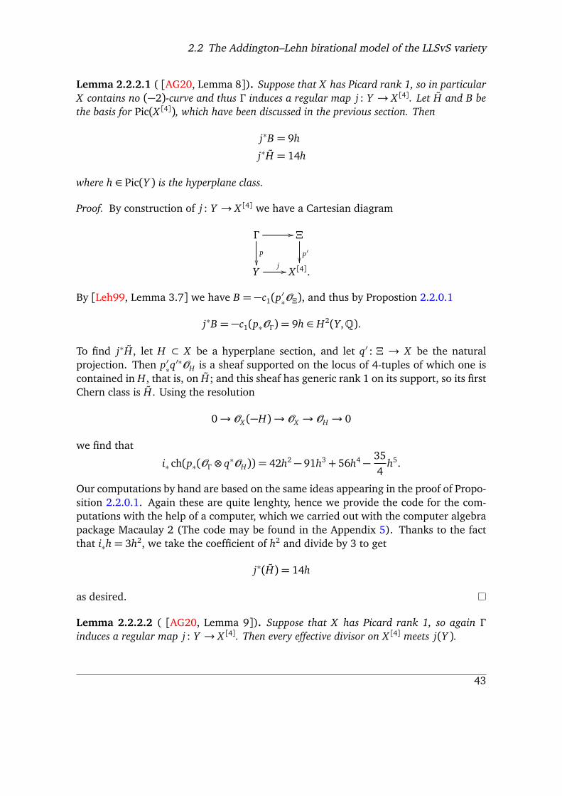
Proof. By construction of j : Y ! X [4] we have a Cartesian diagram
� //
p✏✏
⌅
p0✏✏
Yj
// X [4].
By [Leh99, Lemma 3.7] we have B = �c1(p0⇤O⌅), and thus by Propostion 2.2.0.1
j⇤B = �c1(p⇤O� ) = 9h 2 H2(Y,Q).
To find j⇤H, let H ⇢ X be a hyperplane section, and let q0 : ⌅ ! X be the naturalprojection. Then p0⇤q
0⇤OH is a sheaf supported on the locus of 4-tuples of which one iscontained in H, that is, on H; and this sheaf has generic rank 1 on its support, so its firstChern class is H. Using the resolution
0!OX (�H)!OX !OH ! 0
we find that
i⇤ ch(p⇤(O� ⌦ q⇤OH)) = 42h2 � 91h3 + 56h4 �354h5.
Our computations by hand are based on the same ideas appearing in the proof of Propo-sition 2.2.0.1. Again these are quite lenghty, hence we provide the code for the com-putations with the help of a computer, which we carried out with the computer algebrapackage Macaulay 2 (The code may be found in the Appendix 5). Thanks to the factthat i⇤h= 3h2, we take the coefficient of h2 and divide by 3 to get
j⇤(H) = 14h
as desired.
Lemma 2.2.2.2 ( [AG20, Lemma 9]). Suppose that X has Picard rank 1, so again �induces a regular map j : Y ! X [4]. Then every effective divisor on X [4] meets j(Y ).
43
2 The periods of the Lehn–Lehn–Sorger–van Straten variety
Proof. First we calculate the movable cone of X [4], applying Bayer and Macrì’s result(cf. § 2.2.1) with d = 7 and n = 4. Then d(n� 1) = 21 is not a perfect square; and thePell equation (2.11) 3X 2 � 7Y 2 = 1 has no solution, as we see by reducing mod 3; sowe are in case (c). The minimal positive solution to X 2 � 21Y 2 = 1 is X = 55, Y = 12.This satisfies X ⌘ 1 (mod 3) rather than X ⌘ �1 (mod 3). Thus the movable cone isspanned by
H and 55H � 84B.
The same information can in principle be obtained from work of Markman [Mar11],which does not use Bridgeland stability conditions, but [BM14b] was easier to under-stand for the author.Next we need to know that if D is an effective divisor on X [4] and M is movable, thenq(D,M) � 0, where q is the Beauville–Bogomolov–Fujiki pairing. This follows fromTheorem 2.2.1.2. In fact we do not need the full strength of Boucksom’s result: Indeed,since M is moving we can find representatives of D and M (or better one of its multiples)so that their intersection is of codimension 2 and the computation of q(D,M) reducesto the value of a volume form on their intersection, which is positive (more details canbe found in the proof of [BHT15, Theorem 7]12).Now if an effective divisor D on X [4] does not meet j(Y ), then j⇤(D) = 0, so from Lemma2.2.2.1 we know that D is a multiple of 9H � 14B. But we have
q(H, H) = 14 q(H,B) = 0 q(B,B) = �6,
and thus
q(9H � 14B, H) = 126 q(9H � 14B, 55H � 84B) = �126,
so nomultiple of 9H�14B pairs non-negatively with both walls of themovable cone.
We are now ready to complete the
Proof of Proposition 2.2.0.5. From [AL17, §3]we know that the open immersion t : Z0!X [4], restricted to Y0 := Y \ Z0, agrees with the map j : Y0! X [4] induced by I� . If X hasPicard rank 1, then Y0 = Y by Lemma 2.2.0.4. The open immersion t : Z0 ! X [4] givesa birational map Z ππÀ X [4]. Because Z and X [4] are minimal models, this birationalmap is biregular on an open set W containing Z0 whose complement has codimensionat least 2 in both Z and X [4]. If Z \ Z0 has any component of codimension 1, then sodoes W \ Z0, and taking its closure in X [4] we get an effective divisor that does not meetj(Y ), contradicting Lemma 2.2.2.2.
12The assumption of uniruledness for the divisor is not needed in the argument.
44
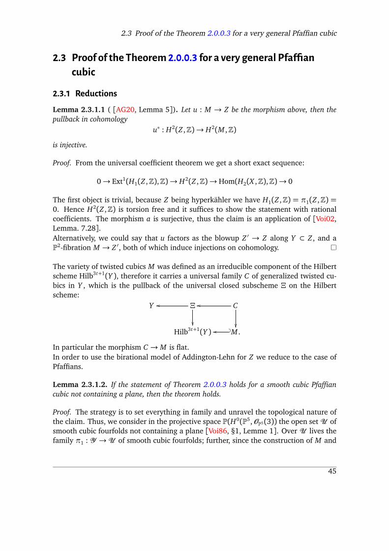
2.3 Proof of the Theorem 2.0.0.3 for a very general Pfaffian cubic
�.� Proof of the Theorem �.�.�.� for a very general Pfa�fiancubic
�.�.� Reductions
Lemma 2.3.1.1 ( [AG20, Lemma 5]). Let u : M ! Z be the morphism above, then thepullback in cohomology
u⇤ : H2(Z ,Z)! H2(M ,Z)is injective.
Proof. From the universal coefficient theorem we get a short exact sequence:
0! Ext1(H1(Z ,Z),Z)! H2(Z ,Z)! Hom(H2(X ,Z),Z)! 0
The first object is trivial, because Z being hyperkähler we have H1(Z ,Z) = ⇡1(Z ,Z) =0. Hence H2(Z ,Z) is torsion free and it suffices to show the statement with rationalcoefficients. The morphism a is surjective, thus the claim is an application of [Voi02,Lemma. 7.28].Alternatively, we could say that u factors as the blowup Z 0 ! Z along Y ⇢ Z , and aP2-fibration M ! Z 0, both of which induce injections on cohomology.
The variety of twisted cubics M was defined as an irreducible component of the Hilbertscheme Hilb3t+1(Y ), therefore it carries a universal family C of generalized twisted cu-bics in Y , which is the pullback of the universal closed subscheme ⌅ on the Hilbertscheme:
Y ⌅oo
✏✏
Coo
✏✏
Hilb3t+1(Y ) M .? _oo
In particular the morphism C ! M is flat.In order to use the birational model of Addington-Lehn for Z we reduce to the case ofPfaffians.
Lemma 2.3.1.2. If the statement of Theorem 2.0.0.3 holds for a smooth cubic Pfaffiancubic not containing a plane, then the theorem holds.
Proof. The strategy is to set everything in family and unravel the topological nature ofthe claim. Thus, we consider in the projective space P(H0(P5,OP5(3)) the open setU ofsmooth cubic fourfolds not containing a plane [Voi86, §1, Lemme 1]. Over U lives thefamily ⇡1 : Y !U of smooth cubic fourfolds; further, since the construction of M and
45

2 The periods of the Lehn–Lehn–Sorger–van Straten variety
Z works in family, we get smooth families over U :
Y
!!
M
✏✏
// Z
}}
U .
(2.13)
In addition, we get the flat family C ⇢ Y ⇥U M . Thanks to Ehresmann’s theorem wefind open sets Ui inU , over which the families Y ,M and Z are trivialised as C1-fibrebundles and we can choose Ui so that the families are simultaneously trivialised.The sheaves on U whose stalks are cohomology (respectively topological K–theory)rings of the fibres are local systems of lattices for each family.At the same time the Fourier-Mukai functor involved and the basic operations as push-forward and pullback give rise to morphisms of local systems. Let us discuss this indetail.Let f : X ! Y be a projective morphism between two smooth families of projectivevarieties over a common base B
Xf
//
p
Y
q~~
B
(2.14)
and we consider the constant sheaves ZX and ZY on the two families. We start withthe pullback in cohomology. Every constant Z-valued function from Y determines byprecomposing with f a constant function on Y , which corresponds to the natural mor-phism of sheaves
ZY ! f⇤ZX .Fibrewise it is the pullback f ⇤ on the 0-degree cohomology
H0(Yb,ZY ) = (q⇤ZY )b! (q⇤ f⇤ZX )b = (p⇤ZX )b = H0(Xb,ZX ).
In general, we consider the Leray spectral sequence relative to the Diagram (2.14)
Ep,q2 = Rpq⇤R
q f⇤ZX ) Rp+qp⇤ZY .
The morphism we are looking for is the composition by proper base change
Rpq⇤ZcY ! Rpq⇤R0 f⇤ZX = Ep,0
2 ! Rpp⇤ZXwhere the second morphism is the edge morphism from the first quadrant spectral se-quence
Ep,02
// //
ed ge map++
Ep,01
� �// Rpp⇤ZX .
46

2.3 Proof of the Theorem 2.0.0.3 for a very general Pfaffian cubic
As we already pointed it out, for projective smooth varieties the pushforward in coho-mology is just given by the action of the pullback twisted by Poincaré duality.The last thing that has to be discussed is the cup product by the class of the curves[Cb] 2 H6(Yb ⇥ Mb,Z). Since the family C ! U is flat, it gives rise to a flat sectionof the local system of H6(Yb ⇥ Mb,Z), so that the cup product is a morphism of localsystems.
�.�.� Proof of Theorem �.�.�.� for a very general cubicFor the reader’s convenience we reproduce here the statement of the theorem.
Theorem 2.0.0.3. Let
�K : Ktop(A ) ⇢ Ktop(Y )! Ktop(M)
be the map on topological K-theory induced by the Fourier–Mukai kernel I_C (�3h) 2 Db(Y⇥M). Then the map
c1 ��K : Ktop(A )! H2(M ,Z) (2.4)
restricts to a Hodge isometry
h�2 ��1i?⇠�! u⇤(H2(Z ,Z)), (2.5)
with the Euler pairing on the left-hand side and the opposite of the Beauville–Bogomolov–Fujiki pairing on the right.
The strategy is to compare the morphism (2.4) of Theorem 2.0.0.3 to the composition:
[I⇠]? ⇢ Ktop(X )I_⌅�! Ktop(X [4])
c1�! H2(X [4],Z),which is known to be a Hodge isometry; here ⇠ ⇢ X is a subscheme of length 4 and⌅ ⇢ X ⇥ X [4] is the universal subscheme.
We consider the functor Db(M)! Db(Y ) induced by IC ⌦OY (2h), the functor Db(Y )!Db(X ) induced by I� , their composition
Db(M)IC (2h)���! Db(Y )
I��! Db(X ), (2.15)
and its left adjoint
Db(X )I_� [2]��! Db(Y )
I_C (�5h)[4]�����! Db(M), (2.16)
which it will later be convenient to rewrite as
Db(X )I_� (�2h)[2]�����! Db(Y )
I_C (�3h)[4]�����! Db(M). (2.17)
47
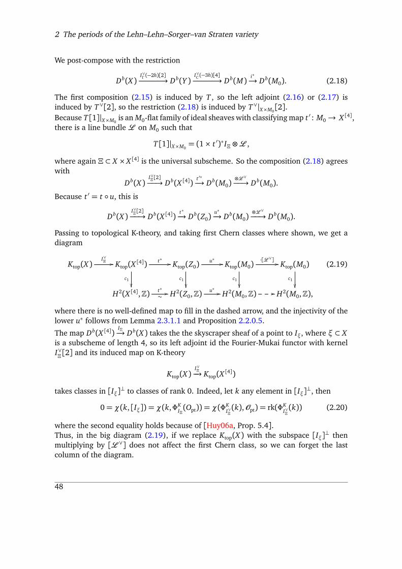
2 The periods of the Lehn–Lehn–Sorger–van Straten variety
We post-compose with the restriction
Db(X )I_� (�2h)[2]�����! Db(Y )
I_C (�3h)[4]�����! Db(M)i⇤�! Db(M0). (2.18)
The first composition (2.15) is induced by T , so the left adjoint (2.16) or (2.17) isinduced by T_[2], so the restriction (2.18) is induced by T_|X⇥M0
[2].Because T[1]|X⇥M0
is anM0-flat family of ideal sheaves with classifyingmap t 0 : M0! X [4],there is a line bundle L on M0 such that
T[1]|X⇥M0= (1⇥ t 0)⇤ I⌅ ⌦L ,
where again ⌅ ⇢ X ⇥ X [4] is the universal subscheme. So the composition (2.18) agreeswith
Db(X )I_⌅ [2]��! Db(X [4])
t 0⇤�! Db(M0)
⌦L_��! Db(M0).
Because t 0 = t � u, this is
Db(X )I_⌅ [2]��! Db(X [4])
t⇤�! Db(Z0)
u⇤�! Db(M0)
⌦L_��! Db(M0).
Passing to topological K-theory, and taking first Chern classes where shown, we get adiagram
Ktop(X )I_⌅
// Ktop(X [4]) t⇤//
c1✏✏
Ktop(Z0)u⇤
//
c1✏✏
Ktop(M0)·[L_]
//
c1✏✏
Ktop(M0)
c1✏✏
H2(X [4],Z) t⇤
⇠// H2(Z0,Z) u⇤
// H2(M0,Z) // H2(M0,Z),
(2.19)
where there is no well-defined map to fill in the dashed arrow, and the injectivity of thelower u⇤ follows from Lemma 2.3.1.1 and Proposition 2.2.0.5.
The map Db(X [4])I⌅�! Db(X ) takes the the skyscraper sheaf of a point to I⇠, where ⇠ ⇢ X
is a subscheme of length 4, so its left adjoint id the Fourier-Mukai functor with kernelI_⌅[2] and its induced map on K-theory
Ktop(X )I_⌅�! Ktop(X [4])
takes classes in [I⇠]? to classes of rank 0. Indeed, let k any element in [I⇠]?, then
0= �(k, [I⇠]) = �(k,�KI⌅(Opt)) = �(�K
I_⌅(k),Opt) = rk(�K
I_⌅(k)) (2.20)
where the second equality holds because of [Huy06a, Prop. 5.4].Thus, in the big diagram (2.19), if we replace Ktop(X ) with the subspace [I⇠]? thenmultiplying by [L_] does not affect the first Chern class, so we can forget the lastcolumn of the diagram.
48
2.3 Proof of the Theorem 2.0.0.3 for a very general Pfaffian cubic
The composition
[I⇠]? ⇢ Ktop(X )I_⌅�! Ktop(X [4])
c1�! H2(X [4],Z)is a Hodge isometry by O’Grady’s classic calculation (cf. Propostion 1.2.4.2). Moreoverthe map t 0⇤ is an isomorphism on H2, so the big diagram (2.19) gives a Hodge isometryfrom [I⇠]? ⇢ Ktop(X ) to u⇤(H2(Z0,Z)) ⇢ H2(M0,Z). Because M \ M0 and Z \ Z0 havecodimension at least 2, this is the same as u⇤(H2(Z ,Z)) ⇢ H2(M ,Z).If we take (2.18), pass to topological K-theory, and include first Chern classes, we get adiagram
Ktop(X )I_� (�2h)
// Ktop(Y )I_C (�3h)
// Ktop(M) i⇤//
c1✏✏
Ktop(M0)
c1✏✏
H2(M ,Z) i⇤
⇠// H2(M0,Z).
(2.21)
As discussed in Proposition 2.2.0.2 the Fourier-Mukai functor
Db(X )I_� (�2h)[4]�����!A
is an equivalence.We claim that the induced map on topological K-theory takes [I⇠] to our class �2��1. To
see this, first observe that the functor Db(Y )I� (�h)���! Db(X ) takes the skyscraper sheaf of a
point Oy to some I⇠, so its right adjoint Db(X )I_� (�2h)[4]�����! Db(Y ) takes I⇠ to the projection
of Oy into A . In K-theory we have [Oy] = [O`(2)]� [O`(1)], where ` is a line on Y , sothe class of the projection of Oy is �2 ��1.Thus, in our second big diagram (2.21), the first map takes [I⇠]? isometrically to (�2��1)? ⇢ Ktop(A ) ⇢ Ktop(Y ). We conclude that themap (2.4) takes (�2��1)? isometricallyto u⇤(H2(Z ,Z)), as desired.This concludes the proof of the main theorem.
�.�.� Proof of Theorem �.�.�.� for a very general cubic
For the reader’s convenience we reproduce here the statement of the theorem.
Theorem 2.0.0.2. The pullback
u⇤ : H2(Z ,Z)! H2(M ,Z)
is injective, and the map[C]⇤ : H4(Y,Z)! H2(M ,Z) (2.2)
49
2 The periods of the Lehn–Lehn–Sorger–van Straten variety
restricts to a Hodge isometry
[C]⇤ : H4prim(Y,Z)
⇠�! u⇤(H2
prim(Z ,Z)), (2.3)
with the intersection pairing on the left-hand side and the opposite of the Beauville–Bogomolov–Fujiki pairing on the right.
By our discussion in §2.3.1, to prove Theorem 2.0.0.2 it is enough to show that fora single cubic Y , the map (2.2) takes H4
prim(Y,Z) into u⇤(H2prim(Z ,Z)) and respects the
pairings. We deduce this from Theorem 2.0.0.3 when Y is not in any Noether–Lefschetzdivisor.Because Y is Noether–Lefschetz general, the transcendental lattice of h�2 � �1i? ⇢Ktop(A ) is h�1,�2i?. The transcendental lattice of H2(Z ,Z) is at least contained inH2
prim(Z ,Z), so the Hodge isometry (2.5) takes h�1,�2i? into u⇤(H2prim(Z ,Z)); but they
are primitive sublattices of the same rank, so (2.5) gives an isomorphism between them.So we need to compare the action of (2.4) on h�1,�2i? with the action of (2.2) onH4
prim(Y,Z). In the diagram (1.2), we know from [AT14, Prop. 2.3] that v takes h�1,�2i? ⇢Ktop(A ) isometrically to H4
prim(Y,Z) ⇢ H⇤(Y,Q). To finish proving Theorem 2.0.0.2, itremains to show that the maps
H4prim(Y,Z)! H2(M ,Q)
induced by v(I_C (�3h)) 2 H⇤(Y ⇥ M ,Q) and [C] 2 H6(Y ⇥ M ,Z) are the same. To seethis, observe that
ch(IC) = 1� [C] + higher-order terms,ch(I_C ) = 1+ [C] + higher-order terms.
The action of the map induced by v(I_C (�3h)) on an element ↵ 2 H4prim(Y ) can be de-
scribed as follows: First we multiply ↵ by (tdY )1/2 and ch(OY (�3h)), which are polyno-mials in the hyperplane class h 2 H2(Y,Z) and thus have no effect on ↵. Then we mapto H⇤(M ,Q) using ch(I_C ), which yields [C]⇤↵+ higher-order terms. Then we multiplyby (tdM)1/2, which does not affect the leading term [C]⇤↵. Then we take the degree-2part, leaving [C]⇤↵ as desired.
In the end we record the following corollary, that can be easily deduced from the aboveresult.
Corollary 2.3.3.1. The Beauville-Bogomolov square of the natural polarization of Z is 2.
Proof. Via the isometry (2.3) we can identify the polarization of Z with the element�1+�2, which is perpendicular to �2��1 in A2 = h�2,�1i. Its square is therefore 2.
50

�Birationalmodels of the LLSvS variety
As an application of Theorem 2.0.0.3 from the previous chapter, we characterise forwhich cubic fourfolds Y the LLSvS variety is birational to the punctual Hilbert schemeof some K3 surface or isomorphic to a moduli space of (twisted) sheaves on a K3 surface(see Theorem 3.1.3.8 below).In order to do so we have to unravel the deep and mysterious bond entangling cubicfourfolds and K3 surfaces, and more in general hyperkähler varieties, as initiated inHassett’s thesis and then developed by many other people. Both objects (cubic fourfoldsand hyperkähler varieties) have a very rich geometry, what makes this an active andwide field of research with many directions. We focus on what we think is necessary notonly to understand, but also to appreciate the topic. The author had indeed the pleasureto attend the conference “School on Birational Geometry of Hypersurfaces” in Gargnanodel Garda1 and indeed our exposition is much indebted to the lecture notes [Huy18],which we recommend for a more comprehensive treatment of the subject. Importantreferences are [Huy], [MS18], and all the original references therein, above all [Has18].
�.� Cubic fourfolds and associatedK�s
�.�.� Theperiods of K� surfaces
K3 surfaces have a very rich geometry and in the last decades were a hot topic of re-search. We report here quickly the results we will need in the following.Recall that complex K3 surfaces are defined as complex compact manifolds of dimension2 with trivial canonical bundle and trivial irregularity. A classical deep result is thatthese surfaces are always Kähler, so that their cohomology has Hodge decomposition.However, not all of them are projective.The Hodge diamond of a K3 surface looks like:
11 20 1
1
1https://sites.google.com/site/gargnano2018/
51

3 Birational models of the LLSvS variety
where we have suppressed the odd cohomology because it is trivial.The integral second cohomology group of a K3 surface S equipped with the intersectionform is an even unimodular lattice of signature (3,19) and thus it is isomorphic to
H2(S,Z)' U�3 � E�28 (�1) =: ⇤
where U is the hyperbolic plane and E8 the lattice associated to the correspondingDynkin diagram.Any primitive element ` 2 ⇤with square `2 = d 2 2Z lies in the same orbit for the actionofO(⇤) ( [Huy16, Corollary 14.1.10]), its orthogonal complement is of fixed isomorphictype
`? ' U�2 � E�28 (�1)�Z(�d)' (e+d2f )? =: ⇤d ⇢ ⇤.
where e and f are generators of a copy of U .For K3 surfaces one can reconstruct the isomorphism type of the surface just from theHodge structure on the second cohomology group, in other words a Torelli-type theoremholds in this context. More precisely:
Theorem 3.1.1.1 ( [Huy06b, Theorem 1.3]). Given two K3 surfaces S and S0.
S ' S0 , There exists a Hodge isometry H2(S,Z)' H2(S0,Z).
In order to understand if two K3 surfaces are derived equivalent, one has to look ata larger lattice. As we have seen in Chapter 1, the whole integral cohomology can beequipped with the Mukai pairing, which agrees with the intersection form on H2(S,Z).This can be computed as:
h(v0, v2, v4), (w0,w2,w4)i= v0w4 + v2w2 + v4w0
and thusH⇤(S,Z) = U�4 � E�28 =: ⇤.
We endow H⇤(S,Z) with a pure (effective) Hodge structure of weight 2 by imposing the(2,0)-part equal to H2,0(S,Z).Now we can state the following result known as derived Torelli theorem.
Theorem 3.1.1.2 ( [Huy06b, Theorem 5.13]). Let S and S0 be two K3 surfaces, then
Db(S)' Db(S0), There exists a Hodge isometry H⇤(S,Z)' H⇤(S0,Z).
TwistedK� surfaces
Definition 3.1.1.3. A twisted K3 surface (S,↵) consists of a K3 surface S and an element↵ 2 H2(S,O ⇤S )tor. An isomorphism of twisted K3 surfaces (S,↵) and (S0,↵0) is an isomor-phism f : S
⇠�! S0 such that f ⇤↵0 = ↵.
52
3.1 Cubic fourfolds and associated K3s
Remark 3.1.1.4. Note that since we are working with complex K3 surfaces, the torsionpart of the group H2(S,O ⇤S ) is isomorphic to the Brauer group of isomorphism classes ofsheaves of Azumaya algebras.
These data determine, as sketched here (for details [HS05, § 2]), a Hodge structure ofK3-type on the Mukai lattice H⇤(S,Z) and a derived category of twisted sheaves, forwhich a Torelli theorem holds.Given ↵ as in the definition, we can consider a Cech 2-cocycle {↵i jk}i jk 2 � (Ui jk,O ⇤S )and twisted sheaves (Ei,'i j) where Ei are coherent sheaves on the open sets Ui and'i j : Ei|Ui j
⇠�! Ej|Ui j
are isomorphisms that satisfy a cocycle condition twisted by ↵:
'ii = id, 'i j = '�1ji , 'i jk �' jki �'ki j = ↵i jk.
Such sheaves form an abelian category Coh(S, {↵i jk}i jk), of whichwe consider the boundedderived category Db(S, {↵i jk}i jk). The construction of the latter does not depend actuallyon the choice of the representing cocycle but just on the class ↵.The exponential sequence gives the surjection H2(S,R)ê H2(S,O ⇤S ), but since our ob-ject of interest is the torsion part, we note that rational cohomology factors through
H2(S,Q)ê H2(S,O ⇤S )tor.
We consider a lifting B 2 H2(S,Q) of ↵ along this morphism and the unique Hodgestructure H(S,↵,Z) of K3 type given by imposing H2,0(S,↵,Z) = Cexp(B)� = C(�+�^B) in H⇤(S,Z). Here � is a non-trivial holomorphic 2-form on S. The Hodge structure isnot independent of the choice of B, but to two different choices of the B-field correspondisometric Hodge structures.A Torelli theorem holds for twisted K3 surfaces as well.
Theorem 3.1.1.5 ( [Huy06b, Theorem 6.2]). Let (S,↵) and (S0,↵0) be two twisted K3surfaces, then the derived categories Db(S,↵) and Db(S0,↵0) are equivalent if and only ifthere exists a Hodge isometry H(S,↵,Z)' H(S0,↵0,Z) preserving the natural orientation.
�.�.� Cubic fourfolds
The Hodge diamond of a smooth cubic fourfold is
11
0 1 21 1 011
53
3 Birational models of the LLSvS variety
where we left out the odd cohomology, because it is trivial. The middle cohomologygroup is torsion free and, equipped with the intersection form, is a unimodular oddlattice of signature (2,21), thus
H4(Y,Z)' (1)�21 � (�1)�2 =: �
where (1)�n, respectively (�1)�n, denotes the lattice of rank n, whose quadratic form isrepresented by the identity matrix, respectively by minus the identity matrix ( [Has18,Proposition 2.1.2]). Its primitive cohomology, which is the orthogonal complement ofthe square of the hyperplane class, is
H4prim(Y,Z)' U�2 � E�28 � A2 =: � .
The square of the hyperplane class h can be realised as the element (1,1,1) 2 (1)�3 ⇢ � ,for details we refer to [Huy, page 23].For cubic fourfolds, a Torelli theorem holds [Voi86] which says that two smooth cu-bic fourfolds are isomorphic exactly when they have isometric Hodge structures on theprimitive middle cohomology. Later we will see a formulation in terms of the periodmap in Theorem 3.1.2.3.
Moduli spaces and the period map The structure of the coarse moduli space and theperiod domain for cubic fourfolds has been investigated by Hassett.
The former is constructed with standard GIT technology as the quotient of the openlocus U ⇢ |OP5(3)| of smooth cubic fourfolds modulo the action of the projective lineargroup PGL(6):
M :=U //PGL(6).
It is a smooth quasi-projective variety of dimension 20.In contrast, one can consider the classifying space of Hodge structures on the abstractlattice � of cubic fourfold type
D := {x 2 P(� ⌦C)| (x , x)2 = 0, (x , x)> 0},
the so-called period domain. Indeed for a smooth cubic fourfold we have seen that H3,1
is spanned by a unique (3,1)-form !, which satisfies ! ^! = 0 for type reasons, and! ^ ! is a volume form, therefore positive. Given H1,3(Y ) one reconstructs the wholeHodge structure using the relations
H3,1 = H1,3
H2,2 = (H3,1 � H1,3)?.
54

3.1 Cubic fourfolds and associated K3s
In virtue of the Baily-Borel theorem one can then show that the quotient of D by theaction of the orthogonal group
O(� ) := {g 2 O(� )| g((1,1,1)) = (1,1,1)}
is a smooth quasi-projective variety C ( [Has18, Proposition 2.2.1]), which is actuallyisomorphic to D/O(� ) as well. 2
Any cubic forufold Y with a so-called marking, that is an isomorphism the choice of anisomorphism � : H4(Y,Z) ⇠�! � , determines a point in D, namely �(H1,3(Y )). Thanksto Voisin Torelli theorem it descends to an injective map, which is actually is an openimmersion of analytic spaces [Voi86]. By applying results by Borel, Hassett proved thatthe period map is actually algebraic [Has18, Proposition 2.2.3] and the complement isdefined by algebraic equations [Has18, Corollary 2.2.4].The theorem has been improved and the complement has been described, as we willsee in Theorem 3.1.2.3.
Hassett divisors We introduce now some divisors on the moduli spaces of cubic four-folds. Usually they are named after Hassett, who was the first to define them and inves-tigate them systematically in his PhD thesis [Has18].A cubic fourfold Y is said to be special of discriminant d if there exists a primitive rank2 sublattice K in H2,2(Y,Z) that contains the square of the hyperplane section h2 andhas discriminant d. The choice of such a sublattice K is called a labelling. Special cubicfourfolds of discriminant d, or better their periods, determine a divisor Cd in C , whichHassett proved to be non-empty exactly when d satisfies:
d > 6 and d ⌘ 0 or 2 (mod 6). (⇤)
Example 3.1.2.1. As smooth cubic fourfolds satisfy the integral Hodge conjecture ([Voi07]), finding a labelling amounts to find a surface, that is not cohomologous to acomplete intersection. We present these classical examples:
• Cubic fourfolds containing a plane are exactly the special cubic fourfolds of dis-criminant 8 . Indeed, let Y be a smooth cubic fourfold and E a projective planesitting in Y . Then the self-intersection product of E on Y is equal to the secondChern class c2(NE|Y ) of the normal bundle. Using the normal short exact sequence
0!TE !TY |E !NE|Y ! 0
2Indeed any isometry g of � extends to an isometry of � mapping (1,1,1) 7! ±(1,1,1) according towhether the action on the discriminant group A� ' Z/3Z is ± id. Then O(� ) is the kernel of thenatural map O(� ) ! O(A� ) which has in index 2 in O(� ), but � id acts trivially on D and the twoquotients are the same.
55

3 Birational models of the LLSvS variety
we can express hE, Ei in terms of the cohomology of E and get rid of the embed-ding. More precisely:
hE, Ei= 6h2 + 3hKE + K2E ��E.
where �E denotes the topological Euler characteristic of E. The intersection prod-uct restricted to the lattice K = hH2, Ei has therefore Gram matrix
K =h2 E
h2 3 1E 1 3
.
where obviously 1 = hE,h2i is the degree of E. Hence the discriminant is 8 andwe have proven that cubic fourfolds containing a plane lie in C8. For the otherinclusion we refer to [Voi86, §3].
• Similarly one shows that the divisor C14 is the closure of smooth cubic fourfoldscontaining a smooth rational normal scroll of degree 4.
Remark 3.1.2.2. A priori, for smooth cubic fourfolds two labellings K and K 0 with samediscriminant d may differ, nonetheless Hassett exploited the action of the orthogonalgroup of � to get that, loosely speaking, there is an isometry of � fixing (1,1,1) takingK to K 0 (cf. [Huy18, Lemma 1.4].
The Torelli theorem has been further improved and in this set up we have the followingtheorem:
Theorem 3.1.2.3 ( [Laz10, Loo09]). The period map induces an algebraic open embed-ding, which is an isomorphism onto the complement of C2 and C6:
P : M⇠�!C \ (C2 [C6)
In light of this theorem it is customary, as we will do, to identify isomrphism classes ofcubic fourfolds with their periods.
�.�.� AssociatedK� surfaces
There is an important link between K3 surfaces and cubic fourfolds based on their co-homology lattices. Let Y be a smooth cubic fourfold and S be a K3 surface. As we haveseen, H2(S,Z) and H4(Y,Z)prim look similar in the sense that they have the same rank,signature and, after a Tate-twist, the same Hodge numbers. Nevertheless, they are stillvery different because the first lattice is even and the second is odd. The way out comes
56

3.1 Cubic fourfolds and associated K3s
to relate primitive cohomology for K3 surfaces with the cohomology of special cubicfourfolds. If d is an even number satisfying
d/2 is not divisible by 9 or any odd prime p ⌘ 2 (mod 3), (⇤⇤)
then and only then there exists a K3 surface S with a polarisation of degree d such that
⇤ � ⇤d ' �d ⇢ � .
This is the content of [Has00, Proposition 5.1.4] and [Huy18, Lemma 1.10], it is anapplication of Nikulin’s results on primitive embeddings of even lattices in connectionwith the Torelli theorems.
Remark 3.1.3.1. Behind this purely lattice-theoretic reasoning there is a nice geometricinterpretation for the mysterious bond between K3 surfaces and cubic fourfolds. If Yis a rational cubic fourfold so that there exists a birational map ⇢ : Y ππÀ P4, then onecan resolve ⇢ as a composition of blow-ups and blow-downs along smooth centres byan application of the Weak Factorisation Theorem ( [Wo03, AKMWo02]). In this wayone cooks up a bunch of K3 surfaces S1, ...,Sm and T1, ..., Tn such that there is a Hodgeisometry
H4(Y,Z)� H2(S1,Z)� ...� H2(Sm,Z) = H2(T1,Z)� ...� H2(Tn,Z).This idea was in effect fundamental in the milestone work of Griffiths and Clemenson the non-rationality of the cubic threefold. In this context curves, thus the Torelli-theorem for curves, were playing a major role. (For more details we point to [Has16,§ 3.1])
Example 3.1.3.2. This principle is well illustrated in the case of a cubic fourfold Y ,which contains two different projective planes P1 and P2. Such a cubic fourfold is knownto be rational, indeed there is a natural birational map:
P1 ⇥ P2 ππÀ Ywhich associates to every pair of points (P1, P2) the third point lying on the intersectionof Y and the line through P1 and P2. The indeterminacy locus of such a map is a K3surface S, the blow-up in S resolves the map.
To put everything on a general footing we need to consider larger lattices. For a K3surface we have already discussed the Mukai lattice H(S,Z). For a cubic fourfold Ywe have introduced in Chapter 1 the lattice Ktop(AY ), now we discuss its arithmeticproperties.We have already discussed the classes �1,�2 and that their orthogonal complementis Hodge isometric to the primitive cohomology of the cubic fourfold (see Proposi-tion 1.3.2.2). The Mukai lattice Ktop(A ) of a cubic fourfold is isomorphic as abstractlattice to ⇤ ( [Huy18, Lemma 1.18]).
57
3 Birational models of the LLSvS variety
In this way, Hprim(Y,Z) is naturally embedded in a lattice abstractly isomorphic to ⇤specularly as for a K3 surface S the lattice H2(S,Z) is embedded in H(S,Z).Definition 3.1.3.3 ( [Huy18, Definition 1.23]). Let Y be a smooth cubic fourfold and letS be a K3 surface
• S and Y are said to be associated if there exists a Hodge isometry
H(S,Z)' Ktop(A ).
• Let L be a polarisation on S. The polarised K3 surface (S, L) and Y are said to beassociated if there exists an embedding
H2(S,Z)prim ,! H4(Y,Z)prim ⇢ Ktop(A ).
• Let ↵ be an element in H2(S,O ⇤S )tor. The twisted K3 surface (S,↵) and Y are said tobe associated if there is a Hodge isometry
H(S,↵,Z)' Ktop(A ).
A comment is in order.
Remark 3.1.3.4. If the polarised K3 (S, L) is associated to a cubic fourfold Y , so is S.Indeed, one can extend any isometry between the primitive cohomology to the wholecohomology group H. Moreover, we point out that if a K3 surface S is associated to acubic fourfold Y , then it is projective. Indeed, we can find in H1,1(S,Z) = H1,1(Y,Z) apositive class, which in turn is a polarisation on S. Further, if a K3 surface S is associatedto a cubic fourfold, then one can find a K3 surface S0 with a polarisation L, so that thepolarised K3 surface (S0, L) is associated to Y (cf. [Huy18, Proposition 1.25]). In virtueof this observation, later we will treat just polarised K3 surfaces.
Example 3.1.3.5. It is not always obvious to find geometrically associated K3 surfaces.For a Pfaffian smooth cubic fourfold Y we have seen in Chapter 2 the construction of aK3 surface X of degree 14. X is indeed associated to Y 3. Thus, all Pfaffian cubics liein the divisor C14 and form a dense locus in it, though not open as recently discoveredin [BRS15, Theorem 3.7].Let us consider the condition:
In the prime factorization of d/2,primes p ⌘ 2 (mod 3) appear with even exponents. (⇤⇤0)
Theorem 3.1.3.6 ( [Huy18, Corollary 2.17]). Let Y be a smooth cubic fourfold.
• Y has an associated K3 surface S if and only if Y is in Cd for some d satisfying (⇤⇤).
• Y has an associated twisted K3 surface (S,↵) if and only if Y is in Cd for some dsatisfying (⇤⇤0).
3Indeed, Beauville and Donagi showed that H4(Y,Z)prim ' H2(F,Z)prim, where F ' X [2], so thatH2(X ,Z)prim ⇢ H2(F,Z)prim ' H4(Y,Z)prim.
58
3.1 Cubic fourfolds and associated K3s
Hyperkähler varieties associated to cubic fourfolds Another fine invariant associated toany cubic fourfold is given by its Fano variety of lines. Indeed, one can even provethe Voisin Torelli theorem for cubic fourfold using the Torelli theorem of hyperkählermanifolds as in [Cha12].The key point is the result from Beauville-Donagi which says that Fano variety are indeedhyperkähler. The original argument by Beauville and Donagi was to show that the Fanoof the Pfaffian is in effect the punctual Hilbert scheme of the naturally associated K3and concluded that every Fano is hyperkähler of K3[2]–type. The question was settledby Addington in [Add16], who introduced the condition
d is of the form2n2 + 2n+ 2
a2for some n, a 2 Z. (⇤⇤⇤)
and showed the following (the twisted result was proven by Huybrechts).
Theorem 3.1.3.7 ( [Add16, Theorem 2], [Huy17a, Theorem 1.3]). Let Y be a smoothcubic fourfold not containing a plane and F its Fano variety of lines.
(a) F is birational to a moduli space of sheaves on a K3 surface if and only if Y 2 Cd forsome d satisfying (⇤⇤).
(b) F is birational to a moduli space of twisted sheaves on a K3 surface if and only ifY 2 Cd for some d satisfying (⇤⇤0).
(c) F is birational to the Hilbert scheme of two points on a K3 surface if and only ifY 2 Cd for some d satisfying (⇤⇤⇤).
Let us introduce a new condition
d is of the form6n2 + 6n+ 2
a2for some n, a 2 Z. (⇤⇤⇤0)
On top of this result, we have
Theorem 3.1.3.8 ( [AG20, Theorem 3]). Let Y be a cubic fourfold not containing a plane— that is, not lying in C8 — so the symplectic eightfold Z is defined.
(a) Z is birational to a moduli space of sheaves on a K3 surface if and only if Y 2 Cd forsome d satisfying (⇤⇤).
(b) Z is birational to a moduli space of twisted sheaves on a K3 surface if and only ifY 2 Cd for some d satisfying (⇤⇤0).
(c) Z is birational to the Hilbert scheme of four points on a K3 surface if and only ifY 2 Cd for some d satisfying (⇤⇤⇤0).
59

3 Birational models of the LLSvS variety
The key ingredient for such theorems is naturally the Torelli theorem for hyperkählervarieties and in particular for K3[n]-varieties.
Remark 3.1.3.9. The number of polarisations of an associated K3 to a cubic fourfoldmay be the maximum possible, that is 20 [Awa20]. For d satisfying (⇤⇤) but not (⇤⇤⇤)the Fano variety is not isomorphic to the punctual Hilbert scheme of the associated K3s.On the other hand if a K3 surface S with Picard number one is associated to a cubicfourfold in Cd for some d divisible by 6 and satisfying (⇤⇤), then there exist exactly oneother associated K3 surface S0. However, it may happen that Hilb2(S) is not birationalto Hilb2(S0): the precise condition was found by Emma Brakkee [Bra18, Corollary 4.9].It would be useful to have similar results about the Hilbert scheme of 4 points.
Remark 3.1.3.10. It is worthwhile to mention another side of the story that we have nottouched in our presentation of cubic fourfolds. The subject expounded here has been in-vestigated from another perspective and with a different machinery and technology, theBridgeland stability conditions on the Kuznetsov componentA of the derived categoryof a cubic fourfold. For a survey we point to [MS18].The condition (⇤⇤) is very important in light of the wild open conjecture, usually at-tributed to Hassett:
Conjecture 3.1.3.11. Let Y be a smooth cubic fourfold. Then Y is rational if and only ifY lies in Cd for some d satisfying (⇤⇤).
This is equivalent to having an associated K3 surface (in sense of Definition 3.1.3.3)and at the same time to thatA is equivalent to the derived category of a cubic fourfold[MS18, Theorem 3.7].
Remark 3.1.3.12. We have the following chain of implications ( [Huy18, Remark 1.9]):
(⇤⇤⇤)) (⇤⇤)) (⇤⇤0)) (⇤).
Moreover, (⇤⇤⇤0) is strictly stronger than (⇤⇤) but incomparable to (⇤⇤⇤): the first fewds satisfying (⇤⇤⇤) are 14, 26, 38, 42, 62, and 86, whereas the first few ds satisfying(⇤⇤⇤0) are 14, 38, 62, 74, and 86.
�.� Proof of Theorem �.�.�.�We adapt an argument developed in [Add16] and [Huy17b, Proposition 4.1] and pol-ished in [Huy18, §3.2], staying especially close to the latter reference.From Verbitsky’s hyperkähler Torelli theorem [Ver13, Huy12, Loo19] and Markman’swork of the monodromy of manifolds of K3[n]-type [Mar11, §9], we know that if n� 1is a prime power, then two manifolds M and M 0 of K3[n]-type are birational (or bimero-morphic) if and only if there is a Hodge isometry H2(M ,Z) ⇠= H2(M 0,Z). If n� 1 has
60

3.2 Proof of Theorem 3.1.3.8
two or more prime factors there is a more subtle statement, but this does not concernus since the eightfold Z is of K3[4]-type.
As we have seen in Proposition 3.1.3.6, a cubic fourfold Y is in Cd for some d satisfying(⇤⇤) if and only if the Mukai lattice Ktop(A ) is Hodge-isometric to the Mukai latticeH(S,Z) of a K3 surface, and similarly with (⇤⇤0) and the Mukai lattice H(S,↵,Z) of atwisted K3 surface.
If ' : Ktop(A )! H(S,Z) is a Hodge isometry, let v = '(�2 � �1), which is a primitivevector satisfying v2 = 6. Then for a v-generic polarization h 2 Pic(S), the moduli spaceM := Mh(v) of h-stable sheaves with Mukai vector v is a smooth variety of K3[4]-type,and satisfies H2(M ,Z)⇠= v? ⇢ H(S,Z). Thus
H2(Z ,Z)⇠= h�2 ��1i? ⇠= v? ⇠= H2(M ,Z).
Conversely, any Hodge isometry h�2��1i? ⇠= v? extends to a Hodge isometry Ktop(A )!H(S,Z) taking �2 � �1 to ±v by [Nik79, Corollary 1.5.2]: the discriminant group ofthe lattice v? is Z/6 whose automorphism group is ±1. With twisted K3 surfaces theargument is similar. This proves parts (i) and (ii) of Theorem 3.1.3.8.
To prove part (iii), by [Add16, Proposition 5] or by the proof of [Huy18, Proposi-tion 3.4(i)] we see that Z is birational to S[4] for some K3 surface S if and only if thealgebraic lattice Knum(A ) ⇢ Ktop(A ) contains a copy of the hyperbolic plane U whichcontains �2��1; or equivalently, if and only if there there is a vector w 2 Knum(A ) with�(w,w) = 0 and �(w,�2 ��1) = 1.
Remark 3.2.0.1. Huybrechts [Huy18] and many other authors define the Mukai pair-ing on Ktop(A ) as having the opposite sign from the Euler pairing, in order to agreewith the Beauville–Bogomolov pairing on H2 of various hyperkähler varieties, whereasAddington and Thomas [AT14,Add16] define it having the same sign as the Euler pair-ing. In effect, the first convention regards Ktop(A ) as a Hodge structure of weight 2,the second as a Hodge structure of weight 0. In the calculation that follows, to avoidconfusion, we only use Euler pairing and do not mention the Mukai pairing.
If there is such a w, let L = h�1,�2,wi ⇢ Knum(A ), and let n = �(w,�1), so the Grammatrix of the Euler pairing on L is
0@�2 1 n1 �2 n+ 1n n+ 1 0
1A
Thus disc(L) = 6n2 + 6n + 2. Let M be the saturation of L in Knum(A ), let a be theindex of L in M , and let d = disc(M); then a2d = disc(L), so d = (6n2 + 6n + 2)/a2.By [AT14, Proposition 2.5] we have Y 2 Cd .
61
3 Birational models of the LLSvS variety
Conversely, suppose that Y 2 Cd for some d of the form (6n2+6n+2)/a2. We claim thata ⌘ 1 (mod 6): to see this, observe that 6n2+6n+2 is the norm of the primitive vector(n,�n� 1) in the A2 lattice, hence satisfies (⇤⇤) by [Huy18, Proposition 1.13(iii)], so amust be a product of primes p ⌘ 1 (mod 3). Thus d ⌘ 2 (mod 6). Write d = 6k + 2and a = 3m + 1. By [Add16, Lemma 9] there is an element ⌧ 2 Knum(A ) such thath�1,�2,⌧i is a primitive sublattice on which the Gram matrix of the Euler pairing is
0@�2 1 01 �2 10 1 2k
1A .
Then the vectorw := (m� n)�1 + (2m� n)�2 + a⌧
satisfies �(w,w) = 0 and �(w,�2 ��1) = 1, as desired.
62

�The geometry of Z
The results and discussion presented here originated from an attempt to verify a conjec-ture of Voisin regarding hyperkähler varieties in the special of the LLSvS eightfold andto understand the geometry of the Voisin rational map
F ⇥ F ππÀ Z .In the course of this project the problem was solved by Fu, Laterveer and Vial ( [FLV20,Corollary 1]) and several discoveries were made around the Voisin map. Therefore, inorder to get a better picture we will place all of it in a wider context.
�.� Context
�.�.� TheVoisin conjecture on the Chow ring of hyperkähler varietiesAmong all the invariants attached to an algebraic variety, the Chow ring is one of themost difficult to understand. Even for a surface it can be quite hard to describe as aresult by Mumford [Mum68] tells us.
Theorem 4.1.1.1. Let S be a surface. If H2,0 6= 0, then there does not exist a curve j : C ,!S such that j⇤ : CH0(C)! CH0(S) is surjective.
The converse to this statement is known as the Bloch conjecture.For K3 surfaces, Beauville and Voisin [BV04, Theorem 1] described a subring with re-markable properties. Indeed, they proved that the degree 2 part of the subring gener-ated by the Picard group of a K3 surface S is the span of the class of any point on somerational curve on S.This result can be rephrased by saying that any polynomial relation holding for thefirst Chern classes of line bundles in cohomology already holds at the level of Chowtheory. Beauville conjectured a similar statement [Bea07], which was further slightlygeneralised by Voisin in
Conjecture 4.1.1.2. [Voi08] Let X be an algebraic hyperkähler variety. Then any poly-nomial cohomological relation
P([c1(L j)], [ci(TX )]) = 0 in H2k(X ,Q), L j 2 Pic(X )
63
4 The geometry of Z
already holds at the level of Chow groups:
P([c1(L j)], [ci(TX )]) = 0 in CHk(X )⌦Q.She then verified the conjecture in various cases including some Hilbert schemes ofpoints on K3 surfaces and the Fano variety of lines on a cubic fourfold. In a furtherinvestigation of the Bloch-Beilinson conjectural filtration for hyperkähler varieties, sheproposes a way of how to get control of the Chow ring of the LLSvS variety Z by reducingto the known results about the Fano variety of lines F . Indeed, she constructs ( [Voi16,Proposition 4.8]) a rational 6-to-1 map
' : F ⇥ F ππÀ Zand she suggests to study the uniruled branch divisor of a resolution of �.
�.�.� Known resultsAs already said, the major result regarding these questions is for sure the verification ofthe Voisin conjecture for the LLSvS variety. This was achieved in a series of papers byFu, Laterveer, Shen and Vial ( [FLV20] [FLV19] [FLVS17]).
About the Voisin map these various results were achieved by different people. Muratoredetermined the indeterminacy locus of the map:
Theorem 4.1.2.1. [Mur20, Theorem 1.2] The indeterminacy locus of the Voisin rationalmap coincides with the variety I of incidental lines. It is irreducible and of dimension 6.
Chen described its resolution of the indeterminacy locus in terms of extensions of sheaves.
Theorem 4.1.2.2. [Che18, Theorem 1.2] The blow-up of F⇥F along the reduced schemestructure of I resolves the Voisin map.
�.�.� Our resultsOur main result regards the branch divisor of a resolution of the Voisin map.Twisted cubics have Hilbert polynomial 3t + 1, their flat degenerations are called gen-eralised twisted cubics. Generalised twisted cubics on a singular cubic surface of typeA1 fall in three different types, which we are going to call ↵,� , and �. They determinetwo divisors D↵,D� , on Z , see Definition 4.2.1.3.
Theorem 4.1.3.1 ( [Gio20, Theorem 1]). The divisor D ⇢ Z of generalised twisted cubicslying on singular cubic surfaces has two irreducible components
D = D↵ [ D� .
The first component coincides with the uniruled branch divisor of a resolution of the Voisinmap.
64

4.2 The divisor of singular cubic surfaces on the LLSvS eightfold
Besides this, we have some other partial results on the Voisin map. The proof of The-orem 4.1.3.1 is, roughly speaking, based on understanding the fibres of the blow-upmorphism over I \ � where � is the image of the diagonal embedding F ,! F ⇥ F .Pushing the investigation further, we study the fibres over � to get
Theorem 4.1.3.2. Let⇡: BlI(F⇥F)! F⇥F be the blow-up in I with the reduced structureand ' : BlI(F ⇥ F)! Z the resolution of indeterminacy of the Voisin map, then
'(⇡�1(�)) ⇢ Y.
Here Y ⇢ Z is the lagrangian embedding of the cubic fourfold.
We determine the singular locus of the variety of incidental lines.
Organisation of the chapter Section 2 is devoted to the proof of our result about thebranch divisor of a resolution of the Voisin map, whereas in Section 3 we discuss theresults regarding the Voisin map and some possible paths to be investigated in the future.
�.� Thedivisor of singular cubic surfaces on the LLSvS eightfold
�.�.� Basic properties of the LLSvS varietyFirst, we recall some details of the construction of the variety Z from [LLSvS17] thatwe have not yet seen. Let Y ⇢ P(V ) ' P5 be a smooth cubic fourfold not containingany plane and let M be the variety of generalised twisted cubics on Y , that is, theirreducible component of Hilb3t+1(Y ) containing smooth twisted cubics. For any curveC 2 M its linear span E := hCi is a P3 that cuts Y in the cubic surface SC := E\Y . Theseassociations give rise to the diagram
M //
�
$$
P(S3W⇤)
✏✏
Gr(V, 4)
s
TT
where W is the universal quotient bundle over the Grassmannian Gr(V, 4) and the sec-tion s is given by intersecting Y with a P3. The morphism � factors through a smoothirreducible variety Z 0 of dimension 8:
M�
$$
a✏✏
Z 0 b// Gr(V, 4)
65

4 The geometry of Z
where a is an étale locally trivial P2-fibration and b is generically finite [LLSvS17, Theo-rem B]. It is finite over the open set UADE ⇢ Z 0 of surfaces that are either smooth or haveordinary double points. For the complement we have the following estimate [LLSvS17,Corollary 3.11, Proposition 4.2, Proposition 4.3]:
dim(Z 0 \ UADE) 6. (4.1)
The irreducible holomorphically symplectic variety Z is obtained by the contraction⇡ : Z 0 ! Z of the irreducible divisor DnCM ⇢ Z 0 of families of curves that are notarithmetically Cohen-Macaulay [LLSvS17, Theorem 4.11].
Notation The points of the variety M are called generalised twisted cubics. In light ofthe construction above, points of the variety Z 0 correspond to families of flat degener-ations of twisted cubics on Y , while each point on Z determines a class of equivalenceof generalised twisted cubics, the equivalence classes being given by the fibers of themorphism u: M ! Z . In the following we will therefore speak of “families” and “classesof generalised twisted cubics” for the points of Z 0 and Z .
The divisor of singular cubic surfaces The projection P(S3W⇤)! Gr(V, 4) is equivariantfor the natural action of PGL(6). The locus Dsing ⇢ P(S3W⇤) of all singular cubic sur-faces in P(V ) surjects onto the Grassmannian, the fiber over a point W0 is the divisorDsing,W0
⇢ P(S3W ⇤0 ) of singular cubic surfaces in P(W0). Furthermore, Dsing,W0is irre-
ducible [Huy, Theorem 2.2] and locally stratified depending on the singularity typeof the parametrised surfaces, the A1 locus forming an open set in Dsing,W0
. Since Dsingcoincides with the orbit of Dsing,W0
under the action of PGL(6) we conclude that Dsingis an irreducible divisor and the A1-locus is open in it. Pulling back this divisor alongs�b : Z 0 ! P(S3W⇤) and taking advantage of both the finiteness of s�b on the ADE-locusand the estimate (4.1) we get the following
Proposition 4.2.1.1 ( [Gio20, Proposition 2]). Let D0 ⇢ Z 0 be the image under a of thelocus of curves lying on singular cubic surfaces. Then D0 is a divisor. Moreover, the preimageunder s � b of singular cubic surfaces of type A1 is a dense open set in D0.
Analogously, singular cubic surfaces determine a divisor DGr := s�1(Dsing) in Gr(V, 4) anda divisor D := ⇡(D0) in Z . In light of this proposition, when discussing the irreduciblecomponents of D0 it will suffice to treat only the A1 locus.
Twisted cubics on A1-singular cubic surfaces While twisted cubics on smooth cubic sur-faces are a classical subject of study, twisted cubics on surfaces with ordinary doublepoints are well explained in [LLSvS17, § 2.1], whose content we briefly recall here andthen make explicit in the specific case of A1 singularities. For basic facts on the root
66
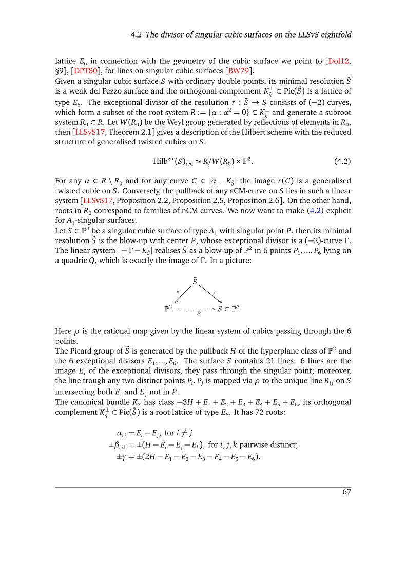
4.2 The divisor of singular cubic surfaces on the LLSvS eightfold
lattice E6 in connection with the geometry of the cubic surface we point to [Dol12,§9], [DPT80], for lines on singular cubic surfaces [BW79].Given a singular cubic surface S with ordinary double points, its minimal resolution Sis a weak del Pezzo surface and the orthogonal complement K?
S⇢ Pic(S) is a lattice of
type E6. The exceptional divisor of the resolution r : S ! S consists of (�2)-curves,which form a subset of the root system R := {↵ : ↵2 = 0} ⇢ K?
Sand generate a subroot
system R0 ⇢ R. LetW (R0) be the Weyl group generated by reflections of elements in R0,then [LLSvS17, Theorem 2.1] gives a description of the Hilbert scheme with the reducedstructure of generalised twisted cubics on S:
Hilbgtc(S)red ' R/W (R0)⇥ P2. (4.2)
For any ↵ 2 R \ R0 and for any curve C 2 |↵ � KS| the image r(C) is a generalisedtwisted cubic on S. Conversely, the pullback of any aCM-curve on S lies in such a linearsystem [LLSvS17, Proposition 2.2, Proposition 2.5, Proposition 2.6]. On the other hand,roots in R0 correspond to families of nCM curves. We now want to make (4.2) explicitfor A1-singular surfaces.Let S ⇢ P3 be a singular cubic surface of type A1 with singular point P, then its minimalresolution S is the blow-up with center P, whose exceptional divisor is a (�2)-curve � .The linear system |� � � KS| realises S as a blow-up of P2 in 6 points P1, ..., P6 lying ona quadric Q, which is exactly the image of � . In a picture:
S⇡
��
r
""
P2 ⇢// S ⇢ P3.
Here ⇢ is the rational map given by the linear system of cubics passing through the 6points.The Picard group of S is generated by the pullback H of the hyperplane class of P2 andthe 6 exceptional divisors E1, ..., E6. The surface S contains 21 lines: 6 lines are theimage Ei of the exceptional divisors, they pass through the singular point; moreover,the line trough any two distinct points Pi, Pj is mapped via ⇢ to the unique line Ri j on Sintersecting both Ei and E j not in P.The canonical bundle KS has class �3H + E1 + E2 + E3 + E4 + E5 + E6, its orthogonalcomplement K?
S⇢ Pic(S) is a root lattice of type E6. It has 72 roots:
↵i j = Ei � Ej, for i 6= j±�i jk = ±(H � Ei � Ej � Ek), for i, j, k pairwise distinct;
±�= ±(2H � E1 � E2 � E3 � E4 � E5 � E6).
67
4 The geometry of Z
We are going to call the roots ↵i, j of type ↵, the roots ±�i, j,k of type � , and the roots ±�of type �. The unique effective root is �, the reflection with center � fixes the roots oftype ↵, whereas its action on roots of type � is:
±�i jk 7! ⌥�lmn
with {i, j, k, l,m,n} = {1,2,3, 4,5, 6}. Hence according to [LLSvS17, Theorem 2.1] theHilbert scheme with the reduced structure is the disjoint union of 51 copies of P2
Hilbgtc(S)red 'G
i, ji 6= j
|↵i j � KS| tG
i, j,kpairwisedistinct
|�i jk � KS| t |� �� KS|.
The curves parametrised by |� �� KS| are not arithmetically Cohen Macaulay and willplay no role in the following. For any curve C in |↵i j�KS| or in |�i jk�KS| the schematicimage r(C) is a generalised twisted cubic on S.An ordered pair (Ei, E j) of distinct lines through the singular point determines the familyof generalised twisted cubics on S corresponding to the linear system |Ei � Ej � KS|.In contrast any triple (Ei, E j, Ek) of pairwise distinct lines through the singular pointdetermines the family of generalised twisted cubic on S corresponding to the linearsystem |H � Ei � Ej � Ek � KS|.We recapitulate what so far has been discussed in the following
Proposition/Definition 4.2.1.2 ( [Gio20, Proposition 3]). Let S be a singular cubic sur-face of type A1, let P be the singular point.
(i) The surface S has 6 distinguished lines E1, .., E6, they are the only lines throughthe singular point. For each pair (Ei, E j) there exists a unique line Ri j meeting Ei
(respectively E j) in a point different from P.
(ii) Each ordered pair (Ei, E j) determines the family of twisted cubics of type ↵ corre-sponding to the linear system |Ei � Ej � KS|. We call such a family of type ↵.
(iii) Each triple (Ei, E j, Ek) determines the family of twisted cubics of type � correspondingto the linear system |H � Ei � Ej � Ek � KS|.1 We call such a family of type � .
(iv) The linear systems |� � �KS| determines a family of generalised twisted cubics on S,which are not arithmetically Cohen-Macaulay. We call these curves of type �.
The general element of the divisor D0 is a family of generalised twisted cubics lying ona singular surface of type A1 and can be of type ↵,� or �.
1The element H is well determined, because H = �� � KS , where � is the unique (�2)-curve of theunique minimal resolution S! S.
68
4.2 The divisor of singular cubic surfaces on the LLSvS eightfold
Definition 4.2.1.3. We define D0↵, D0� , respectively D0�, as the closure of the sets in Z 0 of
families of generalised twisted cubics of type ↵, � , respectively � lying on A1-singular cubicsurfaces. We call D↵, respectively D� , the image ⇡(D0↵) in Z, respectively ⇡(D0�).
Proposition 4.2.1.4 ( [Gio20, Proposition 5]). The closed set D0� is an irreducible divisorin Z 0.
Proof. The divisor D0� parametrises families of generalised twisted cubics which are notarithmetically Cohen-Macaulay, it was already considered in [LLSvS17, Proposition 4.5],where it is shown to be irreducible.
In the next sections we show the irreducibility of D0↵, D↵ (Corollary 4.2.2.3) and of D0� ,D� (Corollary 4.2.2.5).
�.�.� The irreducible components of DThe irreducible component D↵ Let Y be a smooth cubic fourfold not containing a planeand let F be its Fano variety of lines, which is an irreducible holomorphically symplecticvariety of dimension 4. We recall that Voisin [Voi16, Proposition 4.8] constructed adegree 6 rational map
' : F ⇥ F ππÀ Z .The construction goes as follows. Let (l, l 0) be a general point in F ⇥ F . It correspondsto a pair of non-coplanar lines L, L02. After having chosen a point x on L, one takes theresidual conic Qx to L0 of the intersection Y \hx , L0i. The union of Qx and L determinesthen the class of a generalised twisted cubic on the cubic surface S := hL, L0i \ Y . Inother words, the lines L and L0 determine the family |OS(�KS + L � L0)| of generalisedtwisted cubics on S.The indeterminacy locus of ' coincides with the variety I of incident lines, which isirreducible of dimension 6, [Mur20, Theorem 1.2, Lemma 2.3]. The branch divisor ofa resolution of ' is a uniruled divisor, as remarked in [Voi16, Remark 4.10], for detailssee [Mur20, Lemma 4.4]. We denote by Gr := Gr(V, 4) parametrises 3-dimensionalprojective spaces in P5 = P(V ). We consider the rational maps
'0 := ⇡�1 �' : F ⇥ F ππÀ Z 0
:= b �⇡�1 �' : F ⇥ F ππÀ Gr
where ⇡ : Z 0 ! Z is the morphism discussed above and ⇡�1 is its rational inverse map.As natural resolution of the indeterminacy locus of , we consider the closure � of itsgraph with projections p : � ! F⇥ F , q : � ! Gr. We study its points by taking flat limitsalong curves � on F ⇥ F through points where the rational map is not defined.2Here and in the following we will use small letters, as l, to denote lines as points of F and capitalletters, as L, to the denote lines as subschemes of Y .
69
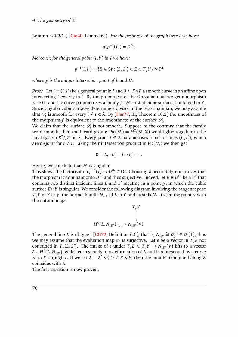
4 The geometry of Z
Lemma 4.2.2.1 ( [Gio20, Lemma 6]). For the preimage of the graph over I we have:
q(p�1(I)) = DGr.
Moreover, for the general point (l, l 0) in I we have:
p�1(l, l 0) = {E 2 Gr : hL, L0i ⇢ E ⇢ TyY }' P1
where y is the unique intersection point of L and L0.
Proof. Let i = (l, l 0) be a general point in I and� ⇢ F⇥F a smooth curve in an affine openintersecting I exactly in i. By the properness of the Grassmannian we get a morphism�! Gr and the curve parametrises a family f : S ! � of cubic surfaces contained in Y .Since singular cubic surfaces determine a divisor in the Grassmannian, we may assumethat St is smooth for every i 6= t 2 �. By [Har77, III, Theorem 10.2] the smoothness ofthe morphism f is equivalent to the smoothness of the surface Si.We claim that the surface Si is not smooth. Suppose to the contrary that the familywere smooth, then the Picard groups Pic(St) = H2(St ,Z) would glue together in thelocal system R2 f⇤Z on �. Every point t 2 � parametrises a pair of lines (lt , l 0t), whichare disjoint for t 6= i. Taking their intersection product in Pic(St) we then get
0= Lt · L0t = Li · L0i = 1.
Hence, we conclude that Si is singular.This shows the factorisation p�1(I)! DGr ⇢ Gr. Choosing � accurately, one proves thatthe morphism is dominant onto DGr and thus surjective. Indeed, let E 2 DGr be a P3 thatcontains two distinct incident lines L and L0 meeting in a point y , in which the cubicsurface E\Y is singular. We consider the following diagram involving the tangent spaceTyY of Y at y , the normal bundle NL|Y of L in Y and its stalk NL|Y (y) at the point y withthe natural maps:
TyY
✏✏
H0(L,NL|Y ) ev// NL|Y (y).
The general line L is of type I [CG72, Definition 6.6], that is, NL|Y⇠= O �2L �OL(1), thus
we may assume that the evaluation map ev is surjective. Let e be a vector in Ty E notcontained in TyhL, L0i. The image of e under Ty E ⇢ TyY ! NL|Y (y) lifts to a vectore 2 H0(L,NL|Y ), which corresponds to a deformation of L and is represented by a curve�0 in F through l. If we set � = �0 ⇥ {l 0} ⇢ F ⇥ F , then the limit P3 computed along �coincides with E.The first assertion is now proven.
70

4.2 The divisor of singular cubic surfaces on the LLSvS eightfold
The limit surface Si is in effect singular in the intersection point y of Li and L0i. Indeed,we may assume Si has one A1-singularity in the point P. In virtue of [Rie92, §2], afterrestricting to an analytic neighbourhood of i, there is a diagram
T r//
✏✏
S
✏✏
(�0, i0)f
// (�, i)
where f : (�0, i0)! (�, i) is a finite Galois cover mapping i0 to i and where T ! �0 is afamily of smooth surfaces such that Tt !S f (t) is an isomorphism for any i0 6= t 2 �0 andTi0 ! Si is the minimal resolution of Si. The surfaces Tt are isomorphic to blow-upsof P2 in 6 points, which are in general position for any t 6= i0, hence the groups Pic(Tt)form a local system over all of �0. The latter becomes trivial, after further shrinking �0
to a contractible neighbourhood of i0. The lines L f (t) ⇢ S f (t) ' Tt form a flat family over�0 \ {i0}. Taking its closure we find a curve X in Ti0 , which completes the family to aflat family over all �0 and corresponds to a section of the local system of Picard groups.The support of X can be either the strict transform L of the line L or the union of L andthe (�2)-curve � , which arises as exceptional divisor of the resolution of Si; the secondcase can happen only if the singular point P lies on L. Thus, we have
X = aL + b�
for some nonnegative integer numbers a and b. Analogously, for the flat limit X 0 of thefamily {L0t}t 6=i we get
X 0 = a0 L0 + b0� . (4.3)
where L0 is the strict transform of L0.Since X , respectively X 0, is the flat limit of the lines {Lt}t 6=i, respectively {Lt}t 6=i, wehave
X 2 = L2t = �1
X · KS = Lt · KSt= 1
(X 0)2 = (L0t)2 = �1
X 0 · KS = L0t · KSt= 1
X · X 0 = 0.
From the first 4 conditions we get
a = a0 = 1; b, b0 2 {0,1}.
71
4 The geometry of Z
The last condition excludes the case b 6= b0, so that
X = L + b� X 0 = L0 + b0� with b = b0 2 {0,1}. (4.4)
From both the remaining cases (i.e b = b0 = 1 or b = b0 = 0) we get that P 2 L \ L0, asdesired.
Let � be a curve as the one in the proof above. Since Z 0 is proper the Voisin map extendsto a well-defined morphism
�0� : �! Z 0.
We are interested in the image of i, which is represented by a family of generalisedtwisted cubics. By the previous lemma we know that any such curve lies on a singularsurface.
Lemma 4.2.2.2 ( [Gio20, Lemma 7]). For the general point i 2 I and the general curve� the limit twisted cubic �0�(i) is of type ↵.
Proof. We may assume that the limit family of twisted cubics lies on a singular surfaceSi of type A1 with one singularity at the point of intersection of L, L0. The point �0�(i) isrepresented by a family of generalised twisted cubics on Si, which in turn correspondsto a linear system A on the minimal resolution S of Si. In contrast, for any other pointt 6= i in � the image �0�(t) consists of the family of curves in |OSt (�KSt + Lt � L0t)|. Afterpassing to a Galois cover of an analytic neighbourhood of i in � as before, we see thatthe linear system A is equal to
|OS(�KS + X � X 0)|= |OS(�KS + L � L0)|
where X and X 0 are the flat limits computed in (4.4). Thus, the limit family �0�(i) is oftype ↵.
In terms of the geometry of Z we have thus proven the following.
Corollary 4.2.2.3 ( [Gio20, Corollary 8]). The closed set D0↵ is an irreducible uniruleddivisor in Z 0. Its image D↵ in Z coincides with the branch locus of a resolution of the Voisinmap.
The irreducible componentD� We consider the variety of triples of lines with non-trivialcommon intersection:
I3 := {(l1, l2, l3) 2 F ⇥ F ⇥ F : L1 \ L2 \ L3 6= ;}.
Lemma 4.2.2.4 ( [Gio20, Lemma 9]). The variety I3 is irreducible of dimension 7.
72

4.2 The divisor of singular cubic surfaces on the LLSvS eightfold
Proof. LetL ⇢ F⇥Y be the universal family of lines on Y parametrised by F , its threefoldproduct fits in the diagram
L⇥L⇥L p//
q✏✏
Y ⇥ Y ⇥ Y
F ⇥ F ⇥ F.
where p and q denote the natural projections. The variety I3 is the image via q ofJ := p�1(�), where Y '� ⇢ Y ⇥Y ⇥Y is the diagonal embedding. Since J is locally cutout by 8 equations, all its irreducible components have dimension greater than or equalto 7. The restriction of q to J is birational and just contracts the diagonal embedding ofL in J :
{(y1, l1, y2, l2, y3, l3) 2 L⇥L⇥L : y1 = y2 = y3 and l1 = l2 = l3} ⇢ J
which has dimension 5. Thus, all irreducible components of I3 have dimension at least7. Via the projection F ⇥ F ⇥ F ! F ⇥ F onto the first two factors the variety I3 is fibredover the irreducible variety I of dimension 6 ( [Mur20, Lemma 2.3]):
p12 : I3! I .
We study its fibres.
• if (l, l 0) lies on the diagonal of F⇥F , that is L = L0, then its preimage is the varietyFL of lines intersecting L.
• In contrast, if (l, l 0) 2 I is a point such that L \ L0 = {y} then the fibre p�112 (l, l0) is
the variety Cy of lines through y .
The variety Cy of lines through a general point y is a curve, which is in general irre-ducible. When it is not a curve, it must be a surface and this is the case just for a finitenumber of points [CS09, Proposition 2.4].The variety FL admits a rational map to L well-defined away from l 2 FL:
FL ππÀ L, r 7! R\ L.
The fibre over a point y 2 L is the variety Cy , thus FL is a surface. It follows that I3 isirreducible.
A general triple (l1, l2, l3) in I3 spans a P3 which intersects the cubic fourfold Y in a sin-gular cubic surface of type A1: the singular point being the unique common intersectionpoint of the three lines. According to our discussion in the previous section, this datadetermines the class of a generalised twisted cubic of type � (cf. Proposition 4.2.1.2).We have therefore constructed a rational map
⇢ : I3 ππÀ Z 0.which is dominant onto D0� . As immediate consequence we get
73

4 The geometry of Z
Corollary 4.2.2.5 ( [Gio20, Corollary 10]). The closed set D0� in Z 0 as well as its imageD� in Z is an irreducible divisor.
Questions Uniruled ample divisors on hyperkähler varieties have been studied by Charles,Mongardi and Pacienza [CMP19] to generalise the results by Beauville and Voisin andto tackle the Beauville-Voisin conjecture and more in general the conjectural existenceof the Bloch-Beilinson filtration.As we have seen, D↵ is a uniruled divisor and it is ample too, because the very generalLLSvS eightfold has Picard number one, thus D↵ needs to be linearly equivalent to amultiple of the polarisation H:
D 2 |nH| for some n.
It would be interesting to compute exactly the integer n. Notice that, knowing n,we would get the Beauville-Bogomolov square of D↵, as we know that the Beauville-Bogomolov square of H is 2 by Corollary 2.3.3.1.In contrast, it is not clear weather D� is uniruled or not as the natural morphism of I3over I is fibred in genus 5 curves.
�.� Other results
�.�.� The singular locus of ILet Y be a cubic fourfold, F its Fano variety of lines. Set I to be the variety of incidentlines:
I = {(l, l 0) 2 F ⇥ F : L \ L0 6= ;}.Here again we we use small letters, as l, to denote lines as points of F and capital letters,as L, to the denote lines as subschemes of Y . Given a line L on Y , its normal bundleNL|Y can be of two types, namely ( [CG72, Definition 6.6]):
(I) NL|Y ' O �2P1 �OP1(1)
(II) NL|Y ' OP1(�1)�O �2P1 (1).
Keeping in mind the distinction in type (I) and (II), we define the variety:
�(I I) = {(l, l 0) 2 F ⇥ F : L = L0, L of type (II)}.
Remark 4.3.1.1. The lines of type I and I I are characterised as follows. The linearspace
\P2LTPY
is a 2-dimensional (respectively 3-dimensional) vector space if L is of type I (respectivelyI I).
74

4.3 Other results
Theorem 4.3.1.2. The singular locus of I is �(I I).
To prove the theorem, we will need to deal with the auxiliary variety
W = {(y, l, l 0) 2 Y ⇥ I : y 2 L \ L0}.
Let ⇡ :W ! I be the natural projection. If we denote by L ⇢ F ⇥Y the universal familyof lines, then W is isomorphic to the fibre product L⇥Y L.A line has Hilbert polynomial t +1 and F is isomorphic to the Hilbert scheme of Y withHilbert polynomial t+1. Analogously, L is isomorphic to the Hilbert scheme Hilb1,t+1(Y )that parametrises flag of schemes in Y with Hilbert polynomials (1, t + 1)3. Thus, onesees that W is isomorphic to the fibre product
Hilb1,t+1(Y )⇥Hilb1(Y ) Hilb1,t+1(Y ).
Lemma 4.3.1.3. The singular locus of W is ⇡�1(�(I I)) =�(I I) ⇥I W .
Proof. We compute the dimension of the tangent space at every point w 2W . Thanks tothe description above, this is an easy task once we employ deformation theory. Indeed,generalising the formula for the tangent space of a flag Hilbert scheme (cf. [Ser06,Remark 4.5.4 (ii)]), one gets that the tangent space at the point w = (y, l, l 0) 2 Wequals the fibre product
TwW = H0(NL|Y )⇥NL|Y (y) TyY ⇥NL0 |Y (y) H0(NL0|Y )
taken over the diagram
H0(L0,NL0|Y )
�0
✏✏
TyY
✏✏
0// NL0|Y (y)
H0(L,NL|Y ) �// NL|Y (y) .
Here the maps �,�0 are given by evaluating global sections at the point y , while , 0
are the natural quotients maps. We observe that H0(L,NL|Y ) is always a vector space ofdimension 4 and so NL|Y (y) is of dimension 3; on the other hand, the rank of � is 3 or4, according to whether L is of type I or I I . Moreover, the kernel of coincides withthe direction spanned by the line L.We proceed with a distinction in cases:3We point to [Ser06, § 4.5] for a general reference for flag Hilbert schemes.
75

4 The geometry of Z
• w= (y, l, l 0)with L and L0 both of type I . Any element in TwW consists of a choiceof a vector v in TyY (4 degrees of freedom) and the liftings of (v) (respectively 0(v)) both 1 degree of freedom. Thus in this case dim TwW = 6.
• w= (y, l, l 0) with L of type I and L0 of type I I . Any element in TwW consists of achoice of a vector v 2 H0(NL0|Y ) (4 degrees of freedom), a choice of a lifting v1 of�0(v) along 0 (1 degree of freedom) and the choice of a lifting of (v1) along �(again 1 degree of freedom). Hence dim TwW = 6.
• w = (y, l, l 0) with L different from L0, both of type I I . A tangent vector to wconsists of a choice of a vector v 2 �1(im�)\ 0�1(im�0) =: X . A quick compu-tation tells us that X can have dimension either 3 or 2, but the former case neverhappens. Indeed �1(im�) is the tangent space of the unique E ' P3 containingL and tangent to Y at any of its point. Clearly E and E0 are different. Thereforedimension of TwW is of dimension 6.
• w = (y, l, l 0) with L = L0 of type I I . We choose an element v 2 �1(im�) \ 0�1(im�0) for which we have 3 degrees of freedom and the two liftings, for eachwe have 2 degrees of freedom. Thus dim TwW = 7.
Since W is irreducible of dimension 6, we conclude that the singular locus consists ofthe preimage of �(I I) along ⇡ as desired.
We are now ready to prove that the singular locus of the variety of incidental lines isthe surface of lines of type I I diagonally embedded in F ⇥ F .
Proof of Theorem 4.3.1.2. Since the morphism ⇡ : W ! I is an isomorphism off � ⇢ I ,from the above lemma we deduce:
I sing ⇢�. (4.5)
Thus we just need to analyse the points on the diagonal. We are going to prove:
dimC(TP I) = 6; 8P 2� \�(I I) (4.6)
dimC(TP I) = 8; 8P 2�(I I). (4.7)
Intuitively, vectors in TP I with P = (l, l 0) parametrise deformations of L and L0 that stillmeet in some point. This amounts to finding a point y 2 L \ L0 such that y admits adeformation with L and, at the same time, with L0, thus for any such vector v 2 TP Ithere exists a y 2 L \ L0 so that (y, l, l 0) 2W deforms in W along v.In other words, TP I contains the subspace in TP(F⇥ F) generated by the images of TQWalong dQ⇡ for all points lying over P
TP I �X
Q2⇡�1(P)
dQ⇡(TQW ).
76
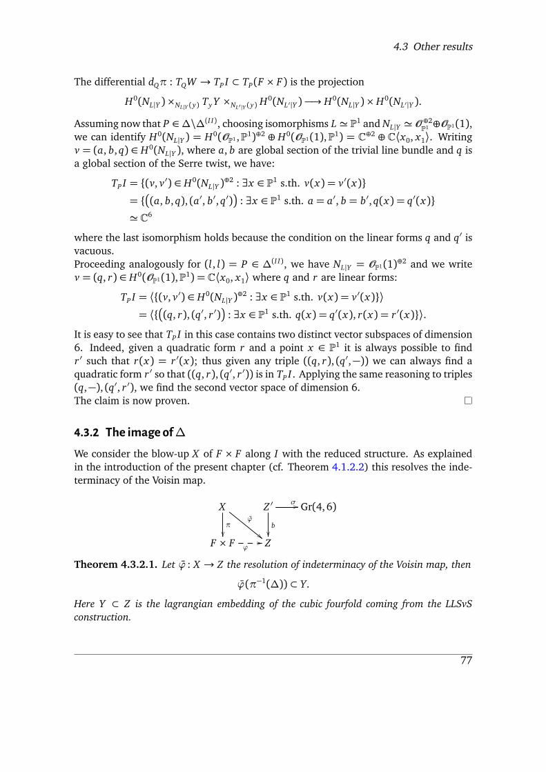
4.3 Other results
The differential dQ⇡ : TQW ! TP I ⇢ TP(F ⇥ F) is the projection
H0(NL|Y )⇥NL|Y (y) TyY ⇥NL0 |Y (y) H0(NL0|Y ) �! H0(NL|Y )⇥ H0(NL0|Y ).
Assuming now that P 2�\�(I I), choosing isomorphisms L ' P1 and NL|Y ' O �2P1 �OP1(1),we can identify H0(NL|Y ) = H0(OP1 ,P1)�2 � H0(OP1(1),P1) = C�2 � Chx0, x1i. Writingv = (a, b,q) 2 H0(NL|Y ), where a, b are global section of the trivial line bundle and q isa global section of the Serre twist, we have:
TP I = {(v, v0) 2 H0(NL|Y )�2 : 9x 2 P1 s.th. v(x) = v0(x)}= {�(a, b,q), (a0, b0,q0)
�: 9x 2 P1 s.th. a = a0, b = b0,q(x) = q0(x)}
' C6
where the last isomorphism holds because the condition on the linear forms q and q0 isvacuous.Proceeding analogously for (l, l) = P 2 �(I I), we have NL|Y = OP1(1)�2 and we writev = (q, r) 2 H0(OP1(1),P1) = Chx0, x1i where q and r are linear forms:
TP I = h{(v, v0) 2 H0(NL|Y )�2 : 9x 2 P1 s.th. v(x) = v0(x)}i= h{�(q, r), (q0, r 0)�: 9x 2 P1 s.th. q(x) = q0(x), r(x) = r 0(x)}i.
It is easy to see that TP I in this case contains two distinct vector subspaces of dimension6. Indeed, given a quadratic form r and a point x 2 P1 it is always possible to findr 0 such that r(x) = r 0(x); thus given any triple ((q, r), (q0,�)) we can always find aquadratic form r 0 so that ((q, r), (q0, r 0)) is in TP I . Applying the same reasoning to triples(q,�), (q0, r 0), we find the second vector space of dimension 6.The claim is now proven.
�.�.� The image of�We consider the blow-up X of F ⇥ F along I with the reduced structure. As explainedin the introduction of the present chapter (cf. Theorem 4.1.2.2) this resolves the inde-terminacy of the Voisin map.
X⇡
✏✏
'
""
Z 0
b✏✏
�// Gr(4,6)
F ⇥ F '// Z
Theorem 4.3.2.1. Let ' : X ! Z the resolution of indeterminacy of the Voisin map, then
'(⇡�1(�)) ⇢ Y.
Here Y ⇢ Z is the lagrangian embedding of the cubic fourfold coming from the LLSvSconstruction.
77
4 The geometry of Z
Proof. First of all, since the singular locus of I coincides with �(I I), the normal bundleNI |F⇥F is a vector bundle of rank 2 outside �(I I) and we interpret the fibres of ⇡ over� 2� \�(I I) as P(NI |F⇥F(�))' P1. Thus ⇡�1(I) is smooth away from ⇡�1(�(I I)).Secondly, ⇡�1(�) is irreducible, as follows from the description of the blow-up givenin [Che18]: its fibres over � \�(I I) are P1 and over �(I I) are P2. Thus ⇡�1(� \�(I I)) isirreducible and its closure must contain ⇡�1(�(I I)).Looking for a contradiction we assume that '(⇡�1(�)) 6⇢ Y , so that the restriction ofthe composition
⌘ : X ! Z ππÀ Z 0 ! Gr .
gives a nontrivial rational map ⇡�1(�) ππÀ Gr. We claim that such a map cannot be welldefined on ⇡�1(�). More precisely we pose
Claim 4.3.2.2. The point⌘(�) corresponds to a linear projective 3-space E⌘(�) that containsthe line L�. Further any point in L� lies in the singular locus of E⌘(�) \ Y .
This leads to the desired contradiction, because there exists no such P3 for a line of typeI (cf. Remark 4.3.1.1).In order to prove the claim, we consider a general point � 2 ⇡�1(�) and its image ⌘(�)and we deduce the properties in the claim by looking at ⌘(�) as limit of various curveslying inside ⇡�1(I), similarly as we did in the previous section. For any point t in theblow-up X , its image ⇡(t) parametrises two lines, which we denote by Lt , L0t; in case tlies in ⇡�1(�) there is actually just one line.Now for a general point � 2 ⇡�1(�) and for any point y 2 L�, we consider the varietyCy of lines through y (which is a curve for the general y 2 Y ) and the curve
�0y = {l�}⇥ Cy ⇢ F ⇥ F.
Such a curve passes through (l�, l�) and we choose a local lifting �y passing through�. By construction of �y and Lemma 4.2.2.1 the point y is singular in E⌘(t) \ Y for any� 6= t 2 �4, thus y must be contained in E⌘(�) \ Y and in its singular locus.Hence the claim is now proven and so is the theorem.
Remark 4.3.2.3. There is a natural anti-symplectic involution � on the LLSvS variety Zand there is the natural involution s on F ⇥ F given by switching the two factors. Theyfit in a commutative diagram
F ⇥ F'
//
s✏✏
Z�
✏✏
F ⇥ F'
// Z .
4Here, E⌘(t) denotes the projective 3-space corresponding to ⌘(t).
78

4.3 Other results
The involution s extends to an involution s on the blow-up X . To see this5, let ⌃ be thecyclic group of two elements, we denote by ↵: ⌃⇥F⇥F ! F⇥F the action of ⌃ on F⇥Fvia�. Notice that I is invariant under the action of⌃ and that the preimage of I under ↵is ⌃⇥ I . By the universal property of the blow-up (e.g. [Har77, § II, Corollary 7.15]) weget a morphism ⌃⇥ X ! X , by assumption this induces an action over the complementof I . Since any two morphism which are equal on a dense open subset must coincide,the action extend to the all of X .In the end, we have a commutative diagram
X'
//
s✏✏
Z�
✏✏
X'
// Z .
We have that the fixed locus of s maps to the fixed locus of �, the previous lemma showsindeed that the fixed locus of s = ⇡�1(�) lands via ' in Y , which is just one of the twocomponents of the fixed locus of �.It would be interesting to give a geometric description of the other component, maybetaking advantage of the divisor D� and its symmetries given by switching lines.
5The argument here is taken by https://mathoverflow.net/questions/122922/group-actions-on-blow-ups.
79

�Appendix
�.� Code for �This is the code used in Chapter 2 to compute the Chern character of p⇤q⇤OX .
loadPackage "Schubert2"P5 = abstractProjectiveSpace’ 5R = intersectionRing P5P5xG26 = flagBundle({2,4}, P5)P5xX = sectionZeroLocus(6*OO_P5xG26(1))P = P5xG26.Bundles_0 ** OO_P5xX -- tautological subbundleQ = P5xG26.Bundles_1 ** OO_P5xX -- quotient bundleGam = degeneracyLocus(1, dual Q ** OO_P5(1), P)p = Gam/P5 -- the projection mapch(p_* OO_Gam) * todd(OO_P5(3))
The output for the last line is:
198
h5 �332
h4 +652
h3 � 27h2 + 12h.
To compute the Chern character of p⇤q⇤OX (H).
OP5xH = OO_P5xX - OO_P5xX(-1) -- this is q^* O_H in the paperch(p_*(OO_Gam ** OP5xH)) * todd(OO_P5(3))
The output for the last line is:
�354
h5 + 56h4 � 91h3 + 42h2.
81

5 Appendix
�.� Cubic surfaces
In the present section we describe a code to find the ideal of a family of cubic surfacesand the families of lines lying on the cubic surfaces!The Voisin map ' : F ⇥ F ππÀ Z is morally of local nature in the sense that can beunderstood at the level of cubic surfaces linear sections of Y . Here we present a piece ofcode we wrote in the attempt to study the map and in particular to determine the imageof the branch divisor of a resolution of such a map. Once we understood that singularcubic surfaces were the key to solve the problem, the code turned out to be useless,because it could not take into account the monodromy of the local system of Picardgroups of the surfaces. We hope nonetheless it might turn useful for further studieswith the opportune modifications and it gave us an idea of the general picture.To study the indeterminacy of the Voisin map, our idea was to find the ideal of a familyof smooth cubic surfaces and of two families of lines such that they are disjoint exceptover the special point. (Un)luckily our idea was flawed and the code turned out uselessfor our purposes. 1
�.�.� Generalities on cubic surfaces
Cubic surfaces are a classical topic of study, for a modern reference we point to thebook [Dol12], in particular §9. Here we give a very brief presentation in order to revisethe bit of theory necessary to explain the strategy of our code.Smooth cubic surfaces S are rational and admit 72 descriptions as blow up of P2 in 6points in general position. In particular if S! P2 is such a blow up, the canonical modelS of S is a cubic surface isomorphic to S and we have a diagram
S
��
'
##
P2 ⇢// S ⇢ P3.
(5.1)
For cubic surfaces with ADE-singularities the situation is similar. Indeed, let S ⇢ P3 bea cubic surface with ordinary double points, then its minimal resolution S ! S can bedescribed in several ways2 as blow-up of P2 in 6 points lying in quasi-general position(cf. [DPT80, Surfaces de del Pezzo III, § 2, Definition 1]), i.e. no line passes through 4points of them. On the other hand, given 6 points in P2 lying in quasi-general position,
1The impossibility to find such a family lead us to upgraded this misconception to the proof of Theo-rem 4.1.3.1
2The exact number depends on the type of singularity.
82
5.2 Cubic surfaces
the canonical model of the blow-up is a cubic surface. We get a diagram
S
��
""
P2 ⇢// S ⇢ P3.
(5.2)
In both diagrams (5.1) and (5.2) the horizontal birational map ⇢ is given by the linearsystem of cubics through the 6 blown-up points. In particular the surface S is the closureof the image of ⇢.The number of lines on a smooth cubic surface is 27. These are the strict transform(along the blow-up ⇡ : S ! S) of the 15 lines through two different blown-up points,the strict transform of the 6 quadrics passing through 5 of the 6 blown-up points, and theimage of the 6 exceptional divisors. For an ADE-surface S the number of lines is smaller,as the 27 P1s with degree 1 with respect to the anti-canonical bundle that we find onS as before may get contracted along the canonical morphism S ! S. In both casesthe lines on the cubic surface are birational transforms along ⇢ of the above mentionedlines and quadrics. With some reasoning we can describe the image of the exceptionaldivisors via ⇢, too.These observations are the base of the following code.
�.�.� Explanation of the codeWe want to write a piece of code that gives (the ideal of) a family of cubic surfaces and(the ideals of) the family of lines on it. We shall present such a family as canonicalmodels of the blow-up in 6 points moving in a fixed P2, thus the family given by theclosure of the image of the map given by the linear system of cubics through the 6moving points. Let us pick 5 fixed points
P1 = (1 : 0 : 0) P1 = (0 : 1 : 0) P1 = (0 : 0 : 1) P4 = (1 : 1 : 1) P6 = (1 : 2 : 3)
The sixth point is moving and we parametrise it as P5 = (1 : a1 : a2) for (a1, a2) 2 A2.3 As generators of the space of cubics through the points we may choose 4 reduciblecubics K1,K2,K3, and K4, which are union of lines, each through 2 distinct points. If weset x1, x2, x3 for the coordinates of the P2 and y1, y2, y3, y4 for the coordinates of P3,then the ideal of the family of surfaces is given by the elimination of the ideal
(y1 � K1(x), y2 � K2(x), y3 � K3(x), y4 � K4(x))
with respect to a global ordering on C[x , y] with yi > x j for any i and j.
3Initially we wrote the code letting two points move P5 = (1 : a1 : a2) and P6 = (1 : a3 : a4), but ourcomputer could not support the complexity of the computations. Thus we adapted the code to justone moving point. This is the reason of the funny notation for the points.Indeed, having two points moving is quite useless, because flat limits exists on curves, but not onsurfaces. P5 is actually moving on a P1!
83
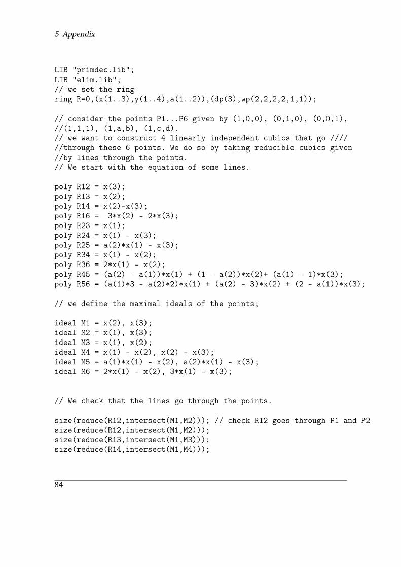
5 Appendix
LIB "primdec.lib";LIB "elim.lib";// we set the ringring R=0,(x(1..3),y(1..4),a(1..2)),(dp(3),wp(2,2,2,2,1,1));
// consider the points P1...P6 given by (1,0,0), (0,1,0), (0,0,1),//(1,1,1), (1,a,b), (1,c,d).// we want to construct 4 linearly independent cubics that go //////through these 6 points. We do so by taking reducible cubics given//by lines through the points.// We start with the equation of some lines.
poly R12 = x(3);poly R13 = x(2);poly R14 = x(2)-x(3);poly R16 = 3*x(2) - 2*x(3);poly R23 = x(1);poly R24 = x(1) - x(3);poly R25 = a(2)*x(1) - x(3);poly R34 = x(1) - x(2);poly R36 = 2*x(1) - x(2);poly R45 = (a(2) - a(1))*x(1) + (1 - a(2))*x(2)+ (a(1) - 1)*x(3);poly R56 = (a(1)*3 - a(2)*2)*x(1) + (a(2) - 3)*x(2) + (2 - a(1))*x(3);
// we define the maximal ideals of the points;
ideal M1 = x(2), x(3);ideal M2 = x(1), x(3);ideal M3 = x(1), x(2);ideal M4 = x(1) - x(2), x(2) - x(3);ideal M5 = a(1)*x(1) - x(2), a(2)*x(1) - x(3);ideal M6 = 2*x(1) - x(2), 3*x(1) - x(3);
// We check that the lines go through the points.
size(reduce(R12,intersect(M1,M2))); // check R12 goes through P1 and P2size(reduce(R12,intersect(M1,M2)));size(reduce(R13,intersect(M1,M3)));size(reduce(R14,intersect(M1,M4)));
84

5.2 Cubic surfaces
size(reduce(R16,intersect(M1,M6)));size(reduce(R23,intersect(M2,M3)));size(reduce(R24,intersect(M2,M4)));size(reduce(R25,intersect(M2,M5)));size(reduce(R34,intersect(M3,M4)));size(reduce(R36,intersect(M3,M6)));size(reduce(R45,intersect(M4,M5)));size(reduce(R56,intersect(M5,M6)));// here we get 0 everywhere, that means, e.g. in the last case that// $R56$ is in $M5\cap M6$.
// Equations of some cubics through all the 6 pointspoly K1 = R12*R34*R56;poly K2 = R13*R24*R56;poly K3 = R12*R45*R36;poly K4 = R14*R25*R36;
//check that the cubics go through the six points.// we define the ideal of the uninon of the six points;ideal MM = intersect(M1,M2,M3,M4,M5,M6);MM = std(MM);ideal KK = K1,K2,K3,K4;KK = std(KK);size(reduce(KK,MM)); // output is ZERO iff KK is in MM
// Finally we get the equations of the cubic, by the elimination trick.ideal I = y(1)-K1, y(2)-K2, y(3)-K3, y(4)-K4;// std(I); // and here I FINALLY get a homogeneous 3-degree//polynomial in y’s, with coefficient in a_iideal C = std(I)[1];
// we compute the discriminant locus of the family of conicsideal t = diff(C,y(1)), diff(C,y(2)), diff(C,y(3)), diff(C,y(4));t = t + C;ideal disc = eliminate(t+(y(1)-1),y(1)*y(2)*y(3)*y(4));disc = intersect(disc, eliminate(t+(y(2)-1),y(1)*y(2)*y(3)*y(4)));disc = intersect(disc, eliminate(t+(y(3)-1),y(1)*y(2)*y(3)*y(4)));disc = intersect(disc, eliminate(t+(y(4)-1),y(1)*y(2)*y(3)*y(4)));disc = std(disc);
85
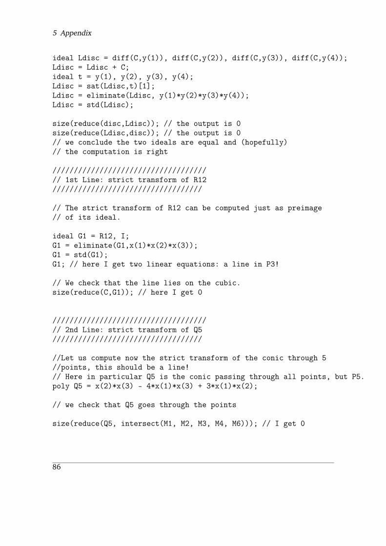
5 Appendix
ideal Ldisc = diff(C,y(1)), diff(C,y(2)), diff(C,y(3)), diff(C,y(4));Ldisc = Ldisc + C;ideal t = y(1), y(2), y(3), y(4);Ldisc = sat(Ldisc,t)[1];Ldisc = eliminate(Ldisc, y(1)*y(2)*y(3)*y(4));Ldisc = std(Ldisc);
size(reduce(disc,Ldisc)); // the output is 0size(reduce(Ldisc,disc)); // the output is 0// we conclude the two ideals are equal and (hopefully)// the computation is right
////////////////////////////////////// 1st Line: strict transform of R12///////////////////////////////////
// The strict transform of R12 can be computed just as preimage// of its ideal.
ideal G1 = R12, I;G1 = eliminate(G1,x(1)*x(2)*x(3));G1 = std(G1);G1; // here I get two linear equations: a line in P3!
// We check that the line lies on the cubic.size(reduce(C,G1)); // here I get 0
////////////////////////////////////// 2nd Line: strict transform of Q5///////////////////////////////////
//Let us compute now the strict transform of the conic through 5//points, this should be a line!// Here in particular Q5 is the conic passing through all points, but P5.poly Q5 = x(2)*x(3) - 4*x(1)*x(3) + 3*x(1)*x(2);
// we check that Q5 goes through the points
size(reduce(Q5, intersect(M1, M2, M3, M4, M6))); // I get 0
86

5.2 Cubic surfaces
//we compute the strict transform of Q5, named G2ideal G2 = Q5, I;G2 = eliminate(G2, x(1)*x(2)*x(3));G2 = std(G2);
// we check that the line G2 lies on the surfacesize(reduce(C,G2)); //here I get 0
///////////////////////////// 4th family: strict transform of a blown-up point and all the others////////////////////////////////
// The exceptional divisor is the projective space of the tangent//space of the blown-up point.// We compute it as the preimage of the square of the maximal ideal//of the point.ideal t = M1*M1;t = t + I;std(t)[1];std(t)[2];std(t)[3];
ideal E1 = std(t)[1], std(t)[2];
///////////////////////////////////////////////////////////// The other exceptional divisors//////////////////////////////////////////////////
// 2nd exceptional divisorideal t = M2*M2;t = t + I;ideal E2 = std(t)[1], std(t)[2];
// 3rd exceptional divisorideal t = M3*M3;t = t + I;ideal E3 = std(t)[1], std(t)[2];
// 4th exceptional divisorideal t = M4*M4;t = t + I;ideal E4 = std(t)[1], std(t)[2];
87

5 Appendix
// 5th exceptional divisorideal t = M5*M5;t = t + I;ideal E5 = std(t)[1], std(t)[2];
// 6th exceptional divisorideal t = M6*M6;t = t + I;ideal E6 = std(t)[1], std(t)[2];
// check that the Ei’s do not intersect, unless (possibly) over the// discriminant locus
// primdecGTZ(E1+E2);// primdecGTZ(E1+E3);// primdecGTZ(E1+E4);// primdecGTZ(E1+E5);// primdecGTZ(E1+E6); // => E1 does not intersect the others// primdecGTZ(E2+E3);// primdecGTZ(E2+E4);// primdecGTZ(E2+E5);// primdecGTZ(E2+E6);// => E2 does not intersect the others// primdecGTZ(E3+E4);// primdecGTZ(E3+E5);// primdecGTZ(E3+E6);// => E3 does not intersect the others// primdecGTZ(E4+E5);// primdecGTZ(E4+E6);//=> E4 does not intersect the others// primdecGTZ(E5+E6);//=> E5 does not intersect the others
88

Theses
• Hyperkähler varieties represent a class of varieties in the realm of algebraic geom-etry with a rich geometry. We study the example of the LLSvS variety Z which isconstructed as a contraction of the variety parametrising generalised twisted cu-bics on a smooth cubic fourfold Y . In Theorem 2.0.0.3 we show that the periodsof Z and Y are the same.
• The LLSvS variety Z of a cubic fourfold Y is deformation equivalent to the Hilbertscheme of 4 points of some K3 surface. In Theorem 3.1.3.8 we determine a con-dition for which the variety Z is birational to such a Hilbert scheme.
• Uniruled divisors drew a lot of attention in the study of Hyperkähler manifolds. InTheorem 4.1.3.1 we give a description the uniruled divisor given by the branch lo-cus of a resolution of the Voisin map: We show that it coincides with an irreduciblecomponent of the divisor determined by singular cubic surfaces on Y .
• Moreover, we show that the divisor determined by singular cubic surfaces on Yhas an other irreducible component and we give a parametrisation of the latter.
89

Bibliography
[Add16] Nicolas Addington. On two rationality conjectures for cubic fourfolds.Math. Res. Lett., 23(1):1–13, 2016. – cited on p. 59, 60, 61, 62
[AG20] Nicolas Addington and Franco Giovenzana. On the period of Lehn, Lehn,Sorger, and van Straten’s symplectic eightfold. arXiv:2003.10984, 2020.– cited on p. 27, 28, 39, 40, 43, 45, 59
[AH59] M. F. Atiyah and F. Hirzebruch. Riemann-Roch theorems for differentiablemanifolds. Bull. Amer. Math. Soc., 65:276–281, 1959. – cited on p. 17
[AH61] M. F. Atiyah and F. Hirzebruch. Vector bundles and homogeneous spaces.In Proc. Sympos. Pure Math., Vol. III, pages 7–38. American MathematicalSociety, Providence, R.I., 1961. – cited on p. 17
[AH62] M. F. Atiyah and F. Hirzebruch. The Riemann-Roch theorem for analyticembeddings. Topology, 1:151–166, 1962. – cited on p. 17, 18
[AKMWo02] Dan Abramovich, Kalle Karu, Kenji Matsuki, and Jarosł aw Wł odarczyk.Torification and factorization of birational maps. J. Amer. Math. Soc.,15(3):531–572, 2002. – cited on p. 57
[AL17] Nicolas Addington and Manfred Lehn. On the symplectic eightfold asso-ciated to a Pfaffian cubic fourfold. J. Reine Angew. Math., 731:129–137,2017. – cited on p. 3, 28, 29, 36, 37, 39, 40, 44
[AT14] Nicolas Addington and Richard Thomas. Hodge theory and derived cat-egories of cubic fourfolds. Duke Math. J., 163(10):1885–1927, 2014. –cited on p. 4, 19, 25, 28, 50, 61
[Awa20] Hanine Awada. Rational cubic fourfolds with associated singular k3 sur-faces, 2020. – cited on p. 60
[BD85] Arnaud Beauville and Ron Donagi. La variété des droites d’une hyper-surface cubique de dimension 4. C. R. Acad. Sci. Paris Sér. I Math.,301(14):703–706, 1985. – cited on p. 3, 13, 27
91

Theses
[Bea83] Arnaud Beauville. Variétés Kähleriennes dont la première classe de Chernest nulle. J. Differential Geom., 18(4):755–782 (1984), 1983. – cited onp. 11, 12, 41
[Bea07] Arnaud Beauville. On the splitting of the Bloch-Beilinson filtration. In Al-gebraic cycles and motives. Vol. 2, volume 344 of London Math. Soc. LectureNote Ser., pages 38–53. Cambridge Univ. Press, Cambridge, 2007. – citedon p. 63
[BHT15] Arend Bayer, Brendan Hassett, and Yuri Tschinkel. Mori cones of holo-morphic symplectic varieties of K3 type. Ann. Sci. Éc. Norm. Supér. (4),48(4):941–950, 2015. – cited on p. 42, 44
[BLM+19] Arend Bayer, Martí Lahoz, Emanuele Macrì, Howard Nuer, AlexanderPerry, and Paolo Stellari. Stability conditions in families, 2019. – citedon p. 28
[BM14a] Arend Bayer and Emanuele Macrì. MMP for moduli of sheaves on K3svia wall-crossing: nef and movable cones, Lagrangian fibrations. Invent.Math., 198(3):505–590, 2014. – cited on p. 41
[BM14b] Arend Bayer and Emanuele Macrì. MMP for moduli of sheaves on K3svia wall-crossing: nef and movable cones, Lagrangian fibrations. Invent.Math., 198(3):505–590, 2014. – cited on p. 44
[Bou04] Sébastien Boucksom. Divisorial Zariski decompositions on compact com-plex manifolds. Ann. Sci. École Norm. Sup. (4), 37(1):45–76, 2004. – citedon p. 42
[Bra18] Emma Brakkee. Two polarized k3 surfaces associated to the same cubicfourfold, 2018. – cited on p. 60
[BRS15] Michele Bolognesi, Francesco Russo, and Giovanni Staglianò. Some lociof rational cubic fourfolds, 2015. – cited on p. 58
[BV04] Arnaud Beauville and Claire Voisin. On the Chow ring of a K3 surface. J.Algebraic Geom., 13(3):417–426, 2004. – cited on p. 63
[BW79] J. W. Bruce and C. T. C. Wall. On the classification of cubic surfaces. J.London Math. Soc. (2), 19(2):245–256, 1979. – cited on p. 67
[CG72] C. Herbert Clemens and Phillip A. Griffiths. The intermediate Jacobianof the cubic threefold. Ann. of Math. (2), 95:281–356, 1972. – cited onp. 70, 74
92

Bibliography
[Cha12] François Charles. A remark on the torelli theorem for cubic fourfolds,2012. – cited on p. 59
[Che18] Huachen Chen. The voisin map via families of extensions, 2018. – citedon p. 5, 64, 78
[CHSW85] P. Candelas, Gary T. Horowitz, Andrew Strominger, and Edward Witten.Vacuum configurations for superstrings. Nuclear Phys. B, 258(1):46–74,1985. – cited on p. 12
[CMP19] François Charles, Giovanni Mongardi, and Gianluca Pacienza. Families ofrational curves on holomorphic symplectic varieties and applications tozero-cycles, 2019. – cited on p. 74
[CS09] Izzet Coskun and Jason Starr. Rational curves on smooth cubic hyper-surfaces. Int. Math. Res. Not. IMRN, (24):4626–4641, 2009. – cited onp. 73
[Deb18] Olivier Debarre. Hyperkähler manifolds, 2018. – cited on p. 41
[Dem92] Jean-Pierre Demailly. Regularization of closed positive currents and inter-section theory. J. Algebraic Geom., 1(3):361–409, 1992. – cited on p. 42
[dJS04] A. J. de Jong and Jason Starr. Cubic fourfolds and spaces of rational curves.Illinois J. Math., 48(2):415–450, 2004. – cited on p. 13, 14
[Dol12] Igor V. Dolgachev. Classical algebraic geometry. Cambridge UniversityPress, Cambridge, 2012. A modern view. – cited on p. 67, 82
[DPT80] Michel Demazure, Henry Charles Pinkham, and Bernard Teissier, editors.Séminaire sur les Singularités des Surfaces, volume 777 of Lecture Notes inMathematics. Springer, Berlin, 1980. Held at the Centre deMathématiquesde l’École Polytechnique, Palaiseau, 1976–1977. – cited on p. 67, 82
[Eis95] David Eisenbud. Commutative algebra, volume 150 of Graduate Texts inMathematics. Springer-Verlag, New York, 1995. With a view toward alge-braic geometry. – cited on p. 38
[FLV19] Lie Fu, Robert Laterveer, and Charles Vial. Multiplicative chow-künnethdecompositions and varieties of cohomological k3 type, 2019. – cited onp. 64
[FLV20] Lie Fu, Robert Laterveer, and Charles Vial. The generalized franchettaconjectur for some hyper-kähler varieties, ii, 2020. – cited on p. 5, 63, 64
93

Theses
[FLVS17] Lie Fu, Robert Laterveer, Charles Vial, andMingmin Shen. The generalizedfranchetta conjecture for some hyper-kähler varieties, 2017. – cited onp. 64
[Ful84] William Fulton. Intersection theory, volume 2 of Ergebnisse der Mathematikund ihrer Grenzgebiete (3) [Results in Mathematics and Related Areas (3)].Springer-Verlag, Berlin, 1984. – cited on p. 31, 34
[GH94] Phillip Griffiths and Joseph Harris. Principles of algebraic geometry. WileyClassics Library. John Wiley & Sons, Inc., New York, 1994. Reprint of the1978 original. – cited on p. 40
[GHJ03] M. Gross, D. Huybrechts, and D. Joyce. Calabi-Yau manifolds and relatedgeometries. Universitext. Springer-Verlag, Berlin, 2003. Lectures from theSummer School held in Nordfjordeid, June 2001. – cited on p. 12
[Gio20] Franco Giovenzana. On the uniruled Voisin divisor on the LLSvS variety.arXiv:2007.07570, 2020. – cited on p. 64, 66, 68, 69, 70, 72, 74
[GS] Daniel R. Grayson and Michael E. Stillman. Macaulay2, a software sys-tem for research in algebraic geometry. Available at http://www.math.uiuc.edu/Macaulay2/. – cited on p. 38
[Har77] Robin Hartshorne. Algebraic geometry. Springer-Verlag, New York-Heidelberg, 1977. Graduate Texts in Mathematics, No. 52. – cited onp. 70, 79
[Has00] Brendan Hassett. Special cubic fourfolds. Compositio Math., 120(1):1–23,2000. – cited on p. 57
[Has16] Brendan Hassett. Cubic fourfolds, K3 surfaces, and rationality questions.In Rationality problems in algebraic geometry, volume 2172 of Lecture Notesin Math., pages 29–66. Springer, Cham, 2016. – cited on p. 57
[Has18] Brendan Hassett. Special Cubic Fourfolds. PhD thesis, University ofChicago, 2018. – cited on p. 51, 54, 55
[HLS19] Andreas Hochenegger, Manfred Lehn, and Paolo Stellari, editors. Bira-tional Geometry of Hypersurfaces. Springer International Publishing, 2019.– cited on p. 24
[HS05] Daniel Huybrechts and Paolo Stellari. Equivalences of twisted K3 surfaces.Math. Ann., 332(4):901–936, 2005. – cited on p. 53
94

Bibliography
[Huy] Daniel Huybrechts. The geometry of cubic hypersurfaces. Available athttp://www.math.uni-bonn.de/people/huybrech/Notes.pdf. –cited on p. 33, 36, 37, 51, 54, 66
[Huy99] Daniel Huybrechts. Compact hyper-Kähler manifolds: basic results. In-vent. Math., 135(1):63–113, 1999. – cited on p. 12
[Huy06a] D. Huybrechts. Fourier-Mukai transforms in algebraic geometry. OxfordMathematical Monographs. The Clarendon Press, Oxford University Press,Oxford, 2006. – cited on p. 14, 17, 22, 23, 24, 48
[Huy06b] D. Huybrechts. The global torelli theorem: classical, derived, twisted,2006. – cited on p. 52, 53
[Huy12] Daniel Huybrechts. A global Torelli theorem for hyperkähler manifolds[after M. Verbitsky]. Number 348, pages Exp. No. 1040, x, 375–403.2012. Séminaire Bourbaki: Vol. 2010/2011. Exposés 1027–1042. – citedon p. 3, 13, 60
[Huy16] Daniel Huybrechts. Lectures on K3 surfaces, volume 158 of CambridgeStudies in Advanced Mathematics. Cambridge University Press, Cambridge,2016. – cited on p. 52
[Huy17a] Daniel Huybrechts. The K3 category of a cubic fourfold. Compos. Math.,153(3):586–620, 2017. – cited on p. 28, 59
[Huy17b] Daniel Huybrechts. The K3 category of a cubic fourfold. Compos. Math.,153(3):586–620, 2017. – cited on p. 60
[Huy18] Daniel Huybrechts. Hodge theory of cubic fourfolds, their fano varieties,and associated k3 categories, 2018. – cited on p. 25, 51, 56, 57, 58, 60,61, 62
[KM98] János Kollár and Shigefumi Mori. Birational geometry of algebraic varieties,volume 134 of Cambridge Tracts in Mathematics. Cambridge UniversityPress, Cambridge, 1998. With the collaboration of C. H. Clemens and A.Corti, Translated from the 1998 Japanese original. – cited on p. 40
[KPS18] Alexander G. Kuznetsov, Yuri G. Prokhorov, and Constantin A. Shramov.Hilbert schemes of lines and conics and automorphism groups of Fanothreefolds. Jpn. J. Math., 13(1):109–185, 2018. – cited on p. 20
[Kuz06] Alexander Kuznetsov. Homological projective duality for grassmanniansof lines, 2006. – cited on p. 39
95
Theses
[Kuz09] Alexander Kuznetsov. Hochschild homology and semiorthogonal decom-positions, 2009. – cited on p. 23
[Kuz10] Alexander Kuznetsov. Derived categories of cubic fourfolds. In Cohomolog-ical and geometric approaches to rationality problems, volume 282 of Progr.Math., pages 219–243. Birkhäuser Boston, Boston, MA, 2010. – cited onp. 24
[Laz10] Radu Laza. The moduli space of cubic fourfolds via the period map. Ann.of Math. (2), 172(1):673–711, 2010. – cited on p. 56
[Leh99] Manfred Lehn. Chern classes of tautological sheaves on Hilbert schemesof points on surfaces. Invent. Math., 136(1):157–207, 1999. – cited onp. 3, 43
[Leh18] Christian Lehn. Twisted cubics on singular cubic fourfolds—on Starr’sfibration. Math. Z., 290(1-2):379–388, 2018. – cited on p. 29
[LLMS18] Martí Lahoz, Manfred Lehn, Emanuele Macrì, and Paolo Stellari. General-ized twisted cubics on a cubic fourfold as a moduli space of stable objects.J. Math. Pures Appl. (9), 114:85–117, 2018. – cited on p. 3, 29, 30, 31,36
[LLSvS17] Christian Lehn, Manfred Lehn, Christoph Sorger, and Duco van Straten.Twisted cubics on cubic fourfolds. J. Reine Angew. Math., 731:87–128,2017. – cited on p. 3, 5, 14, 27, 29, 34, 35, 65, 66, 67, 68, 69
[Loo09] Eduard Looijenga. The period map for cubic fourfolds. Invent. Math.,177(1):213–233, 2009. – cited on p. 56
[Loo19] Eduard Looijenga. Teichmüller spaces and torelli theorems for hyperkäh-ler manifolds, 2019. – cited on p. 60
[LPZ18] Chunyi Li, Laura Pertusi, and Xiaolei Zhao. Twisted cubics on cubic four-folds and stability conditions, 2018. – cited on p. 28, 29
[LPZ20] Chunyi Li, Laura Pertusi, and Xiaolei Zhao. Elliptic quintics on cubic four-folds, o’grady 10, and lagrangian fibrations, 2020. – cited on p. 14
[Mar11] Eyal Markman. A survey of Torelli and monodromy results forholomorphic-symplectic varieties. In Complex and differential geometry,volume 8 of Springer Proc. Math., pages 257–322. Springer, Heidelberg,2011. – cited on p. 13, 42, 44, 60
96

Bibliography
[MS18] Emanuele Macrì and Paolo Stellari. Lectures on non-commutative k3 sur-faces, bridgeland stability, and moduli spaces, 2018. – cited on p. 51, 60
[Muk81] Shigeru Mukai. Duality between D(X ) and D(X ) with its application toPicard sheaves. Nagoya Math. J., 81:153–175, 1981. – cited on p. 14
[Mum68] D. Mumford. Rational equivalence of 0-cycles on surfaces. J. Math. KyotoUniv., 9:195–204, 1968. – cited on p. 63
[Mur20] Giosuè Emanuele Muratore. The indeterminacy locus of the Voisin map.Beitr. Algebra Geom., 61(1):73–88, 2020. – cited on p. 5, 64, 69, 73
[Nik79] V. V. Nikulin. Integer symmetric bilinear forms and some of their geometricapplications. Izv. Akad. Nauk SSSR Ser. Mat., 43(1):111–177, 238, 1979.– cited on p. 61
[O’G] Kieran O’Grady. Compact hyperkähler manifolds: an introduc-tion. Available at http://irma.math.unistra.fr/~pacienza/notes-ogrady.pdf. – cited on p. 12
[O’G97] Kieran G. O’Grady. The weight-two Hodge structure of moduli spaces ofsheaves on a K3 surface. J. Algebraic Geom., 6(4):599–644, 1997. – citedon p. 13, 19, 20, 28
[Pet18] Carolin Peternell. Birational Models for Moduli of Quartic Rational Curves.PhD thesis, Johannes Gutenberg Universitat Mainz, 2018. – cited on p. 14
[Rie92] Oswald Riemenschneider. Special surface singularities: a survey on the ge-ometry and combinatorics of their deformations. Number 807, pages 93–118. 1992. Analytic varieties and singularities (Japanese) (Kyoto, 1992).– cited on p. 71
[Ros82] Jean-Pierre Rosay. Injective holomorphic mappings. Amer. Math. Monthly,89(8):587–588, 1982. – cited on p. 40
[Sch20] Martin Schwald. On the definition of irreducible holomorphic symplecticmanifolds and their singular analogs, 2020. – cited on p. 11
[Ser06] Edoardo Sernesi. Deformations of algebraic schemes, volume 334 ofGrundlehren der Mathematischen Wissenschaften [Fundamental Principlesof Mathematical Sciences]. Springer-Verlag, Berlin, 2006. – cited on p. 75
[Ver13] Misha Verbitsky. Mapping class group and a global Torelli theorem for hy-perkähler manifolds. Duke Math. J., 162(15):2929–2986, 2013. AppendixA by Eyal Markman. – cited on p. 3, 13, 60
97
Theses
[Voi86] Claire Voisin. Théorème de Torelli pour les cubiques de I P5. Invent. Math.,86(3):577–601, 1986. – cited on p. 45, 54, 55, 56
[Voi02] Claire Voisin. Hodge theory and complex algebraic geometry. I, volume 76 ofCambridge Studies in Advanced Mathematics. Cambridge University Press,Cambridge, 2002. Translated from the French original by Leila Schneps.– cited on p. 29, 34, 45
[Voi07] Claire Voisin. Some aspects of the Hodge conjecture. Jpn. J. Math.,2(2):261–296, 2007. – cited on p. 55
[Voi08] Claire Voisin. On the Chow ring of certain algebraic hyper-Kähler man-ifolds. Pure Appl. Math. Q., 4(3, Special Issue: In honor of Fedor Bogo-molov. Part 2):613–649, 2008. – cited on p. 5, 63
[Voi16] Claire Voisin. Remarks and questions on coisotropic subvarieties and 0-cycles of hyper-Kähler varieties. In K3 surfaces and their moduli, volume315 of Progr. Math., pages 365–399. Birkhäuser/Springer, [Cham], 2016.– cited on p. 64, 69
[Wo03] Jarosł aw Wł odarczyk. Toroidal varieties and the weak factorization the-orem. Invent. Math., 154(2):223–331, 2003. – cited on p. 57
98