GEOMETRODYNAMICS OF QUANTUM FIELDS IN BLACK HOLE ANTI-DE SITTER

GEOMETRODYNAMICS OF QUANTUM FIELDS

IN BLACK HOLE ANTI-DE SITTER SPACETIMES

Andrew DeBenedictis

BSc. (Honours), University of British Columbia, 1995

M.%., University of Windsor, 1996

THESIS SUBMITTED IN PARTIAL FULFILLMENT

OF THE REQUIREMENTS FOR THE DEGREE OF

DOCTOR OF PHILOSOPHY

in the Department

of

Ph ysics

@ Andrew DeBenedictis 2000 SIMON FRASER UNIVERSITY

June 2000

All rights reserved. This work may not be reproduced in whole or in part, by photocopy

or other means, without permission of the author.

Nadiorral Likary 1+1 0fca"d.a BWiotheque nationaie du Canada

uisiüons and AcquWi et 8' iographii Senrias seMces bibliographiques 3

The author has granted a non- exclusive licence ailowing the National Li'brary of Canada to reproduce, loan, disûiiute or sell copies of this thesis in microform, paper or electronic formats.

The author retains ownership of the copyright in this thesis. Neither the thesis nor substantial extracts from it may be printed or otherwise repruduced without the author's permission.

L'auteur a accordé une licence non exclusive permettant la Bibliothèque nationale du Canada de reproduire, prêter, distribuer ou vendre des copies de cette thèse sous la forme de microfichelfilm, de reproduction sur papier ou sur format électronique.

L'auteur conserve la propriété du droit d'auteur qui protège cette thèse. Ni la thèse ni des extraits substantiels de ceiie-ci ne doivent être imprimés ou autrement reproduits sans son autorisation.

Abstract

In the context of semi-classical general relativity, an in depth study of quantum effects on

classicai singularity structure is performed. The systern studied is that of an asyniptotically

anti-de Sitter (.4dS) cylindrical black hole spacetime with conforrnally coupled scalars as the

matter field. This fact requires speciai care with boundary conditions which is discussed in

detail.

Thermodynamic properties of torroidd versions of these black holes are first studied.

The free energy and entropy are obtained using simple thermodynamic arguments and the

stability of the black holes is discussed.

The renormalized expectation value (42) = lim,,.y(#(s)~(z')) is cdcdated using

a mode sum decornposition. It is found that the field is divergence free throughout the

spacetime and attains its maximum value near the horizon.

The gravitationai back-reaction wbich this field introduces is aiso calculated. By first calculating the expectation value of the field's stress-energy tensor, (Tt), the Einstein

field equations are solved (to îïrst order in A) and the perturbation on the Kretschmann

scalar is obtained. It is found that near the horizon, the perturbation initidly strengthens

the singularity. Xear spatial infinity, however, curvature is weakened.

Finally, a rnethod of adding successive boundary counter-terms is utilized to renor-

malize the bulk gravitational action in asymptoticdy AdS solutions. It is shown that the

correct conserved quantities of the spacetime are produced and therefore this renormalized

quantity may be viewed as a "gravitationai stress-energy tensor". The resulting stress-energy

tensor yields botli the correct bIack hole energies as weii as terms interpreted as vacuum

Casimir energies of the dual field theory (including a negative energy contribution). This

calcdation is done up to d = 8 (d being the boundary dimension). In light of the anti-de

Sitterjconformai field theory (,\dS/CFT) correspondence, the trace of this quantity yields

the Weyl anomaly of the dual field theory coupled to gravity.

To the memoy o j Burton Seale

who passed away during the production o j this work

and

as a retirement gift to Dr. Anadi Dus: scholar, phdosopher, teocher, and friend.

Acknowledgment s

There are many people whom 1 would like to acknowledge in relation to this work.

1 would first like to thank my senior supervisor, Dr. K. S. Viswanathan for al1 the

help he has given me with this project. 1 feel 1 have learned much under his guidance

and he has greatly aided my understanding of a difficult topic. Dr. Viswvanathan has

been instrumental in the production of this work and our discussions over lunch will

be rnissed. 1 would also like to thank my graduate committee members: Dr. A. Das for stimulating weekly discussions on relativity and for his kindness and friendship

and Dr. H. Trottier for sharing his enthusiasm for physics and teaching. There are

many friends and acquaintances 1 would like to thank al1 of which, 1 regret, can not

be mentioned here due to lack of space. 1 would like to thank the people in P7420: E. Emberly for excellent discussions and bringing some much needed humour (and

Spanish radio) to Ph.D. life and for keeping me up to date on the state of professional

wrestling, J. Wendland and W. Mück for coffee breaks and friendship (thanks, J.W.,

for the coffee machine and spilot). 1 would also like to thank others in our research

group: P. Matlock and Y. Yang, as well as those whose expertise in Pandun were

instrumental to our mission's success: M. Rastan and J. Emerson. Also, my deepest

thanks go to Dr. S. Rangnekar, Sharon, Susan and Candida, whom 1 bothered far

too much and owe many favours to. My good friends C. Magnuson and Governor

Ambrosio should also be acknowledged and very special thanks also go to Eduardo

(continue el buen trabajo) and SVEN. Finally, and above d l , 1 would like to thank

my wife Jennifer for support and encouragement nithout which this project would

not have been possible.

Contents

Approval

Abstract

Dedicat ion

Acknowiedgment s

Contents

List of Figures

1 Introduction

ii

iii

iv

v

vi

viii

1

Brief History and Ovewiew of Black Holes and Singularity Structure

in General Relativity . . . . . . . . . . . . . . , . . . . . . . . . . . . . 3 1.1.1 Singularity Tbeorems . . . . . . . . . . . . . . . . . . . . . . . . 6 Cylindrical Systems in General Relativity . . . . . . . . . . . . . . . . . 8

Structure of Anti-de Sitter and Anti-de Sitter Black Hole Spacetimes . 13

1.3.1 .4nti-de Sitter BIack Holes . . . . . . . . . . . . . . . . . . . . . 17

Black Hole Thermodynamics in Brief . . . . . . . . . . . . . . . . . . . 22

Review of Semi-Classical Geome trodynamics . . . . . . . . . . . . . . . 25

Boundary Counter-Terms and Gravitational Stress-Energy Tensors . . . 38 1.6.1 The boundary counter-tenn method . . . . . . . . . . . . . . . . 40

1.6.2 The AdS/CFT Correspondence . . . . . . . . . . . . . . . . . . 42

List of Figures

. . . . . . . . . . . . . . 1.1 Singularity forming from gravitational collapse 5 . . . . . . . . . . . . . . . . . . . . . . . 1.2 Conjugate point to a surface S 7

. . . . . . . . . . 1.3 hlexican hat potential associated with cosmic strings 12 . . . . . . . . . . . . . . . . . . . 1.4 Penrose diagrams for AdS spacetirne 15

. . . . . . . . . . . . . . . . . . . . . . 1.5 ESU with AdS mapped on to it 16 . . . . . . . . . . . . . . . 1.6 Penrose diagrarns of black string spacetimes 21

. . . . . . . . . . . . . . . . . . 3.1 (42) in cylindrical black hole spacetime 65 . . . . . . . . . . . . . 3.2 (@) in Reissner-Nordstrorn black hole spacetime 65

4.1 Energy density of quantum scalar field . . . . . . . . . . . . . . . . . . 73 . . . . . . . . . . . . . . . . 4.2 Energy density in Schwarzschild spacetime 73

Chapter 1

Introduction

In this thesis studies of quantum effects in black hole spacetimes with negative

cosmological constant are carried out. The work is conducted within the scope of

semi-classical general relativity as ive11 as higher derivative gravity and the anti-de

Sitter/conformal field theory (AdSICFT) correspondence. This work is essentially

divided into two parts. The first part consists of an in depth study of how quantum

effects affect the singularity structure of a classical singular spacetime. The cylindrical

black hole developed by Lemos and Zancbin 111 is chosen as the starting point for the

calculations and this solution will be discussed in some detail later in this chapter.

Some thermodynamic quantities are calculated and cornparisons are made to spheri-

cally symmetric black holes with and without cosmological constant. -4 confornially

coupled quantum field is then introduced via a calculation of the renormalized values

of the field expectation value, (42) = lim,,d(~(x)~(x*)) and the expectation value

of the stress-energy tensor, (T,,). This latter value is then used as a source in the

perturbed Einstein field equations and back-reaction effects are considered.

The motivation is the hope that the studies here will shed some light on

how quantum effects affect the singularity which is predicted by classical general

relativity. Do the semi-classical effects depend on the particular geometry chosen and the presence of a cosrnological constant or are the effects universal? If semi-classical

effects weaken the singularity of al1 black holes then one c m say with some confidence

that quantum effects may remove the singularity.

In the second part of the thesis calculations are done in the conte* of higher

CHAPTER 1. INTRODUCTION 2

derivative gravity and the .MS/CFT correspondence. By adding counter-terms de-

pending on the boundary geometry to the gravitationai action, the mass of higher

dimensional btack holes is calculateci. It is shown that this method generates cor-

rect conserveci quantities for black hole spacetimes of bIack holes up to 9 spacetime

dimensions. The trace of the resultant stress-energy tensor is then expanded about

the boundary coordinate to yield the trace anomaly of the dual field theory. These

methods are useful especially when considering solutions to the field equations with

non-trivial topology (such as Taub-NUT spacetime). These calculations shed some

light on the validity of this scheme to higher dimensions as well as yield some infor-

mation on SUSY Yang-Mills theory and (0,2) tensor multiplet theory.

The conventions here closely follow those of Misner, Thorne and Wheeler's

book Gravitation (21. Briefly, the Riemann tensor in terrns of the connexion is given

by :

where partial derivatives are denoted by commas (covariant derivatives by semi-

colons) and

Greek indices may take on the values O, 1,. . . , D - 1 where D is the total dimension

of the spacetime manifold. Latin indices denote a subspace of the total manifold

(however, unlike 121, the subspace need not necessarily be strictly spacelike). The

metric tensor has signature +2 and units are such that G = c = h = kB = 1. With

these conventions, the Einstein field equations take the form:

with 11 being the cosmological constant. The absolute value of the metric's determi-

nant is denoted by g.

1.1 Brief History and Overview of Black Holes and

Singularity Structure in General Relat ivity

Given the nature of the work in this study, a briefovewiew of the history of black

holes is presented here as well as a review of some of the properties of sinplarities.

For a more detailed exposition on these subjects the reader is referred to 131 and 141.

The study of singularity formation in black hole physics bas an interesting

history. In fact, Einstein himself rejected the idea of a black hole asserting that they

must be unphysical and actually violated the taws of relativity 151.

The thought that such an object may be created within the framework of

general relativity goes back to the original solution of Schwarzschild 161 whicti, in its

most farniliar form is written as:

the coordinates being the standard spherical chart so that r defioes the area of two

spheres. It is irnmediatety obvious that there are two 'trouble spots" in this nietric:

T = O and r = 2 M (or r = 2GM/$ if c and G are not set to unity), and it is this

second position (the "Schwarzschild singularity'') which originally troublcd physicists

niost up until the 1960's.

What Einstein and others ignored in their analysis of gravitational collapse

ivas the possibility of implosion. That is, it !vas thought that matter must ultimately

form a static configuration a t some point during the cotlapse even if the collapse

proceeds wi thin the Schwvarzschild singulari ty.

The first study to seriously consider the possibility of implosion was the clas-

sic study by Oppenheimer and Snyder 171. This study, though greatly idealized, holds

al1 the qualitative features of generic , non-rotational, gravitational colfapse. Oppen-

heimer and Snyder used a pressureless, constant density fluid (dust) as their matter

mode1 and followed the collape from a number of reference frames. They found that,

in a frarne CO-moving Mth the surface of the dust ball, the star Ml1 in fact implode

and (although they did not comment on it at the time) the star will reach a state

of infinite density and zero volume in finite proper time. Purely radial motion of a

CH.4PTER 1 . INTRODUCTION 4

particle on the matter surface may be described by the following geodesic equations:

+ 2 ~ l ( r o / ~ . ~ l - 1 1 ) ' ' ~ [q + (~~/dh!f) (q + sin q)l (1 -5 b)

e =go (1.5~)

d =do, ( l a )

where r, is the radial position of the surface at Schwarzschild time t,. Bo and do are

constant and q parameterizes the collapse from its initial position, r, = TO at q = O

to its termination at the singularity at q = n. Proper time at the surface is given by

the expression:

r = p(q + sin q), 8111

from which it can be seen that the surface reaches T = O in proper time

It is interesting to note that this is the sanie time lapse dernarlded by Newtonian

theoy for free-faIl collapse to infinite density.

Wartime and cold war pressures halted further serious study of singularities

untiL the 1950's. By this time cornputers developed to simulate the complex physics

of hydrogen bomb systerns allowed gravitational collapse to be modeled taking into

account pressure, nuclear reactions, shock waves (which are necessarily absent in pres-

sureless fluids), heating, radiation and m a s ejection. The first such study, conducted

by May and White [SI, showed that, if a star had a m a s much greater than two solar

masses, implosion into a black hole was imminent just as predicted by Oppenheimer

and Snyder. These results were independently obtained in the U.S.S.R. 191.

It is most instructive to study the formation of a black hole utilizing ingoing

Eddington-Finklestein coordinates. In this scheme one replaces the SchwarzschiId

time coordinate in (1.4) with a nul1 coordinate, V , which is constant along radially

CH.4PTER 1. INTRODUCTION

ingoing nul1 geodesics.

v = t + r',

where

The metric (1.4) now takes the form

From this Ive can construct the collapse spacetime diagram shown in figure 1.1 which

demonstrates the qualitative features of collapse forming a singularity.

C' V = const.

Figure 1.1: Gravitationai collapse to form a singularity in ingoing Eddington-Finklestein co-

ordinates. The coordinate V is constant dong ingoing radial n d geodesics. A characteristic

timelike geodesic is shown as a dotted line.

CKAPTER 1. INTRODUCTION

1.1.1 Singularity Theorems

The singularity theorems are a powverful set of theorems regarding the existence

of singularities in general relativity I101. The difficult task of precisely defining a

spacetime singularity is required and much effort has been granted to this task (for

example seeIll1). The definition used here will be a variant of Schmidt's (121:

Definition: 1.1 Let s be an afine parameter describing space-like, null and time-like

geodesics. Suppose that, after finite lapse of afine parameter, one O! these curves

terminates. Further suppose that it is impossible to &end the manifold beyond the

termination point due to infinite curvature. Then that tennination point, dong Iuoth

adjacent tennination points, constitutes a singularity.

Further, the definition of a trapped surface is required:

Definition: 1.2 Let T be a compact, smooth, space-like submanifold. Then, if the

expansion of both sets of future null geodesics orthogonal to T is eueqwhere negatiue,

the region T is a trapped surface.

Qualitatively, the singularity theorems state that the presence of trapped

surfaces necessarily imply the existence of a singularity somewhere in the spacetime

manifold. -4 more technical version of the singularity theorems may be established by

considering the following propositions which are a variant of Wald's [131.

Proposition: 1.1 Let k be a null vector. If Ra8kaka 3 O euerywhere (i-e. satisIy

the weak or strong energy condition) and there is a closed trapped surface T in the

manifold M then there exists a point conjugate to T dong evey future directed null

geodesic orthogonal to T . This conjugate point will be within an afine dàstance 2/c

of T .

The actual definition of the affine distance parameter c is unimportant here and its

non-zero existence is al1 that is required. Conjugate points are defined as points where

neighbouring geodesics converge. A conjugate point to a surface S is the point where

neighbouring geodesics normal to S intersect.

CH.4PTEIZ 1. INTRODUCTION

Figure 1.2: Diagram illustrating key concepts required for the singularity theoreni. An

arbitrary surface is denoteù by S along with a conjugate point q (the neighbouring geodesics,

y, are infinitesimally close on S). In definition 1.2 y represent future nul1 geodesics. The

surface is a trapped surface if q decreases for increasing affine parameter of y. Proposition

1.2 States that for nul1 conjugate geodesics, y may be deformed smoothly into a cime-like

curve. Finally, the singularity theorems state that for S a trapped surface, at least one cuve

(7) possesses finite a f h e length.

Proposition: 1.2 Let S be a space-like two surface and p a point in spacetime. Fur-

ther, let y be a null geodesic cuwe orthogonal to S from S to p. If there is a point

in (S,p) conjvgate (null) to S along p, then there exists a smooth defornation of y

which gives a time-like curue jmm S to p.

One of the singularity theorems may now be stated and proved (this is a variant of

the original theoreni of Penrose (101) (also refer to figure (1.2 for clarity)).

Theorem: 1.1 Let M be a connected, globally hyperbolic spacetime vith non-compact

Cauchy surface C. Suppose RagkakS 2 O for al1 null ka. Suppose also that M contains a trapped surface T. Then, there is a limit on the length of at least one

future directed orthogonal null geodesic jrom T .

CiiA PTER 1. INTRODUCTION 8

Proof: The spacetime is causally simple due to the globally hyperbolic postulate.

Therefore, the boundary of the causal future of 7 (j+(7)) will be E+ (that is, the

causal future minus the chronological future) and will have nul1 geodesic segments

as its generator. These generators will have past endpoints on 7 and which are

orthogonal to 7. If the manifold, M were geodesically (null) complete then, by the

condition ROskokB 2 0, the existence of a trapped surface, and proposition 1.1, there

would be a point conjugate to 7 within an affine distance 2/c at the point where

the nul1 geodesic intersects 7. By proposition 1.2 the point on the geodesic beyond

the conjugate point to 7 would lie in the chronological future of 7 and therefore

each generating segment of j+(7) would have a future endpoint at or before the

point conjugate to 7. In a continuous manner, one could assign an affine parameter

on each nul1 geodesic orthogonal to 7. Consider the mapping B defined by taking

the point p E 7 an affine distance v E [O, b] along one of the future directed nuIl

geodesics orthogonal to 7 and through p. There will be some minimum value of c

(CO, say) since 7 is compact. Then, if bo = 2/co, the mapping B would contain the

j+(T) which tvould be compact as it is a closed subset of a compact set. Consider

now a Cauchy surface C which is not compact and utilize the fact that M admits

a past directed time-like vector field whose integral curves intersect C and intersect

the j+ (7) no more than once. These integral curves define a continuous one-to-one

mapping u : j+ (T) -t C. If j+(7) were compact, its image ol(j+(7)) wvould also

be compact and would be homeomorphic to j+ (7). Now, since C is non-compact,

a( ~ + ( 7 ) ) could not contain the whole of C and must possess a boundary in C. This

is an irnpossibility since ?(7) and therefore u ( j+(T) ) would be a three dimensional

manifold without boundary. The assumption that M is nul1 geodesically complete

(used in the proof that j + ( 7 ) is compact) is incorrect. I .A proof of a similar, more general, theorem which abandons the restriction of

global hyperbolicity may be found in 141.

Cylindrical Systems in General Relativity

Cylindrical symmetry has proved to be a valuable tool for studying and discussing

the internai structure and consistency of general relativity (for example see 11.11, 1151

CH,.IPTER 1. INTRODUCTION

[l61, 1171, 118)). It has also been shown how black string solutions a ise in low energy

string theory as well as how these solutions may be interpreted as black cosmic strings

(191 in the theory of topological defects. In the context of gravitational coliapse, it

bas been shown how cylindrical collapse simulates the astrophysical collapse of a Gnite spindle (201 as tell as how a cylindrical distribution of matter may collapse to

form cylindrical black holes 1301. Since cylindrical systems in gravitation and particle

physics find rnuch relevance in the theory of cosmic strings, a brief review is presented

here for completeness.

Cosmic strings are topotogical defects which arise in quantum field theory

within the context of spontaneously broken symmetries. It is generally believed that

the observed symmetries in particle physics resulted from a much larger syrnmetry

group. Schematically:

where each arrow indicates that a symmetry breaking phase transition has taken

place. At each phase transition there is the potential for the formation of some sort

of defect. This is analogous to the formation of defects in condensed matter systems

such as the rnagnetic flux lines of type II superconductors, the quantized vortex lines

of superfluid 4He and the domain structure of ferromagnetic materials.

In a cosmologicai context, a succession of phase transitions occur as the uni-

verse expands and cools. The tirne at which the strong nuckar force became differ-

entiated from the other forces is an exampte of such a transition. The topological

defects (such as cosmic strings) consist of regions where the vacuum is in its origi-

nal, more symmetric, "old" phase. The occurrence of topological defects is essentially

guaranteed if the universe at some point undergoes a period of rapid cooling such as

is present in the inflationary scenariosI211. -4lthough inflation is not strictly required

for the formation of topological defects, it will briefly be shown below how defect

production rnay be augmenteci by an inflationary period. The importance of such

defects in cosmology has been stuclied in detail 1221 The inflationary scenario arose as a modification to the standard hot big bang

mode1 to help resolve difficulties with the old theou such as the horizon and flatness

problems '. Briefly, the horizon problem arises from the observeci isotropy of the

cosmic microwave background radiation (CMB) which is isotropie within 1 part in

10'. Now, causally connected sections of the horizon of 1 s t photon scattering should

subtend an angle in the sky of approximately

0 IS - - R ' / ~ Z ~ " ~ radians, (1.12)

where Zl is the dimensionless density parameter defined as the density of the universe

divided by the critical density. 21, is the redshift at 1 s t scattering which is approxi-

mately q u a i to 1000 1231. This yields a value of el, x 2" which clearly demonstrates

that the CMB must be arriving from causally disconnected regions. -4 period of infla-

tion when regions which are initiaily causally connected become disconnected would

explain such isotropy. -4 new scenario has also recently been proposed to explain the

horizon problem which involves an effective variable speed of light 1241. This scenario,

in the spirit of a Brane World scenario, possesses sonie desirable features not present

in the standard inflationary scheme.

The flatness problem originates from the observation that the matter density

in the universe is within an order of magnitude of the critical density, that is, S I A. 1.

Howwer, from the Einstein equations with conservation law:

(a(r) being the conformal time scale factor in the Friedmann-Robertson-Walker (FRW) geometry), the Zl = 1 point is an unstable equilibnum point. In order to have R - 1

today it must have been tuned to 11 - 111 5 IO-= a t the Planck time. As will be seen,

inflation rnay offer a solution to this problem as well.

Inflation may be invoked by introducing a scalar inflaton field, a , with appro-

priate potential. The Einstein equations with FRW geometry yield:

lThe idationary mode1 has the potential of solvïng other problems in cosmology as weii.

CHAPTER 1 . INTRODUCTION 11

where dots denote time derivatives. If there is a region where the potential dominates

then the inflaton "fiuid" bas equation of state p = -p. Further, if p is approximately

constant the field will behave as a cosmological constant and, by the Friedmann

equation:

a(r) will increase exponentially. The process eventually terminates due to the slow

evolution of the a field beyond the inflation point.

The flatness problem is naturally resolved in inflation by noting that the

temperature at the onsct of inflation and the temperature near its termination (the

reheating phase) are approximately equai. Now, in the critical case (1.15) becomes

so that

Since during the inflationary process the scale factor grows exponentially, the density

today must be very close to the critical density. An excellent review of the model's

success and shortconiings may be found in 1251

The simplest niodel in which cosmic strings arise is that of the complex scalar

field, t$(x), whose Lagrangian density is given by:

with X and q positive constants. This "blexican hat" potential is shown in figure 1.3.

Although 1.18 is manifestly U(1) (global) invariant, the ground state is not

as the field acquires a vacuum expectation value (VEV) of

The symrnetric vacuum ((01910) = O) is given by the local maximum of the potential

1.18. During a period of rapid cooling, the universe will undergo a phase transi-

tion (V(t$) = V- in the diagram) and cosmic strings will result in regions where the

potential maintains its unstable equilibrium value.

Figure 1.3: Pvle'acan hat potential associateci with cosmic strings. The (true) vacuum

manifold is not simpiy connected. The false vacuum (local maximum) corresponds to a

cosmic string.

At first sight it rnay seem that inflation would act to dilute al1 structure

including topological defects such a s strings. However, there exist scenarios where

defects rnay be formed in abundance duriiig sonie phase of the inflationary stage. It is

possible to introduce couplings between the scalar field rnaking up the cosmic string,

4 and the inflxton field, a, of the forrn

with a and X constant. For small O, energetics dictate that q5 - O. AS u increases, the

point u » fiq is reached and it will then be energetically favourable for 4 to acquire

a non-zero expectation value. This scheme is sirnilar to that described in 1261 and

demonstrates how cosmic string abundance and density may be enhanced through

inflation.

The line element of a standard (non black hole solution) cosmic string is given, in

a cylindrical coordinate chart, by:

where p is the mass per unit length of the string. By noting that (1 - 4p) is just a

constant, it may be seen that the spacetime is flat evqwhere except at r = O. The


only difference between (1.21) and Minkowski spacetime is the presence of an "angular

deficit". That is, although the angular coordinate, 4 runs from O to 2x , the proper

angle in the spacetime manifold possesses range from O to 27~ - 87rp. Cosmic string theory and the theory of cosmological phase transitions is a very

cornplex and rich theory. The cosmic string mode1 presented here is the simplest, and

therefore least realistic, model. For a more in deptli study of these topics the reader

is referred to [271 and (281.

1.3 Structure of Anti-de Sitter and Anti-de Sitter

Black Hole Spacetimes

Anti-de Sitter spacetime (AdS) is the spacetime of constant negative curvature

defined by :

where the coordinates <, reside in a N-dimensional ernbedding spacetime and rrqL is

the radius of curvature of the D = N - 1 climensional XdS spacetime. Generaljy,

there is no global covering of AdS spacetime and at least tivo coordinate charts are

required. Because of this, al1 future references to AdS spacetime will refer to one

half plane of the full AdS structure. This limitation will not affect the results as the

two planes are disconnected. The embedding spacetime has a flat Lorentzian rnetric

structure with line element:

Where n$) is an iV dimensional Minkowski metric with two time-like coordinates.

The surface defined by (1.22) and (1.23) possesses D(D + 1)/2 Killing vectors and is therefore a spacetime of maximai symmetry with symmetry group SO(2, D - 1). That is, the rotationai symmetry of the embedding space. Since much of the work

in this thesis involves a four dimensional spacetime, the rest of this section will be

limited to the case D = 4.


It is useful to study AdS spacetime using the following common parametriza-

t ion:

<O = a-' cos 7 sec

tL = a-'tanpcosB

c2 = a-' tan p i n Bcos 4

t3 = û-l tanpsinBsin4

t4 = a-' sin 7 sec p,

which leads to the following AdS metric:

ds2 = sec2 (p) [-dr2 + dp2 + sin2 p(dB2 + sin2 0 dqb2)] ,

Since the points T = -R and T = A are identified, AdS has the topology S1 x R3 and

therefore possesses the undesirable property of closed tirne-like curves. The standard

procedure for eliminating this problem is to unravel the S1 yielding what is known

as the %niversal covering space" of .4dS where -cm < T < W. These properties are

easily seen in figure 1.4 (see caption). -411 future references to .4dS spacetime will

actually refer to this covering space.

It is also evident from figure 1.4 that AdS spacetirne is not globally hyperbolic

since nul1 infinity ( p = 7r/2 surface) is time-like. To see this consider an initial data

surface in figure 1.4 at r = -T. If the initiai data consists of rnassless matter, there

will be a tirne at T = - ~ / 2 where the data essentially 'Ylows out of the manifold".

Therefore, if one bas complete knowledge of events at a point p in the spacetime then

the infinite Future (or past) of this event cannot be predicted. This problem is further

augrnented by the fact that data or 'hews" may always flow into the manifold at this

boundary. It is this non-global hyperbolicity tvhich requires the implementation of

CHPTER 1. INTRODUCTION

Figure 1.4: Penrose compactification diagrams for (a) anti-de Sitter spacetime (top and

bottom identifiecl) and (b) the universai covering spacetime. The dotted line represents a

characteristic time-like geodesic.

special boundary conditions at nul1 infinity as any qiiantization scheme heavily relies

on the spacetime being globdly hyperbolic. It was shown in [291 that three natural

boundary conditions arise in AdS spacetime when considering quantum fields. The

condition used in most of this work will be the %transparentn boundary condition.

The transparent boundary condition may be realized by noting that AdS spacetime is confomally related to one half of the Einstein static universe (ESU) which is globdly hyperbolic (see figure 1.5). By treating AdS spacetime as half the

ESU ive rnay establish a well defined Cauchy problem. Utilizing this mapping, it can

be seen that any nul1 information which leaves AdS at a time T gets 'f ecycled" by

re-entering at a time r + K. This way one can predict to the infinite future and past

as required for a Cauchy problern. This scheme is only valid for nul1 fields since, as

ma? be seen in figure 1.3, time-like geodesics never reach the p = 7r/2 surface. These

CH.4PTER 1. INTRODUCTION 16

considerations will become important later ivhen quantum field expectation values are

dealt with.

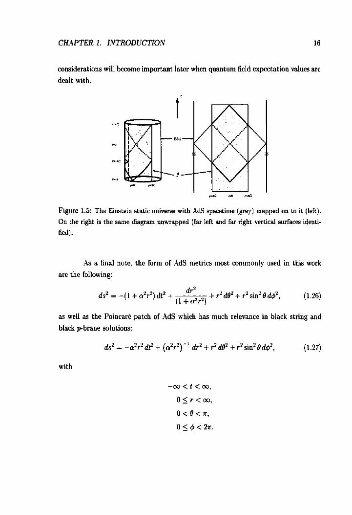
Figure 1.5: The Einstein static universe with AdS spacetime (grey) tnappeci on to it (left).

On the right is the same diagrani unwrapped (far left and fa t right vertical surfaces identi-

fied) .

As a final note, the form of AdS metrics most cornmonly used

are the following:

in this work

(1.26)

as well as the Poincaré patch of AdS which has much relevaace in black string and

black pbrane solutions:


The method of obtaining the Poincaré patch from (1.26) is not difficult although it

will not be presented here as the techaical details detract from the main text. These metrics represent the covering space of AdS spacetime and are of importance as the

coordinates passes simple physical interpretation, T defining the m a of twespheres,

for example.

1.3.1 Anti-de Sitter Black Holes

The coupling of gravity to a negative cosmological constant allows for a much

richer theory of black hales than that of their asymptotically flat counterparts. Some

of these exotic properties will be discussed here with special ernphasis put on black

holes of cylindrical or toroidal symmetry. These objects are not naked singularities

and therefore, although violating the hoop conjecture (which States that no black

hole may form until material has collpasecl within a radius equal to its Schwarzschild

radius), do not violate cosmic censorship. It has also been shown how matter can

coiiapse to form such black holes 1301, 1321. There is much interest in studying the .US class of black holes duc to a nuniber

of properties asymptotically -4dS solutions possess, Asymptotically AdS solutions

are stable even though the energy is unbounded from below (321. .Aho, extended

supergravity theories with O ( N ) symmetry have AdS spacetime as their groiind state.

More recently, .ldS spacetime has appeared in the context of the ?daIdacena conjecture

and -4dS holography 1331, 1341, more of which will be discussed later. Finally, there is

the now famous 2+1 dimensiond MS black hole of Baiiados, Teitelboim and Zanelli

(BTZ black hole) 1351. The four dimensionai Einstein-Hilbert action in the presence of electromag-

netic field is given by:

where A is the cosmological constant, assumeci to be negative in this case. The solution

studied here solves the Einstein-Mauwe!I equations with cylindncal s y m m e t l i.e.

there exists a commuting h o dimensional Lie group of isometries Ga which generates

a space O€ topology R x S1. Toroidal solutions dso exkt and will be studied hi

CiL4PTER 1. INTRODUCTION 18

a thermodynamic context later. A coordinate system is chosen (t, p, <p, 2 ) with the

following ranges:

Solving the Einstein-Mauwell equations utilizing the assurnption that the so-

lution be stationary yields [II

Where AI, Q, and J are the mas, charge, and angular momentum per unit length

of the string respectively. These charges may be deterrnined utilizing a background

subtraction technique of Brown and York 1361. The quantity Q is given by:

The above solution does not dirnensionally reduce to the 3D-BTZ black hole due

to the unavoidable presence of a non-constant dilaton field in the corresponding 3- dimensional reduced action.

In the spacetime considered here, both charge and angular mornentum

are zero yielding the following for (1.31)

An event horizon exists a t p = p~ f - ('"'1'3 Cl and the cosmological constant (which

is negative and necessary for cylindrical black hote solutions), A = -3u2, dorninates

in the limit p + oo giving the spacetime its asymptotically anti-deSitter behaviour.

This metric is exactly of the form which arises naturaily in the study of topologicai

black holes [371 and is similar to a solution derived by Witten when studying -4dS

correspondence and black holes [38). ,inalflical extensions to p < O are possible but

will not be discussed here.


The apparently singular behaviour of the spacetime at p = p~ is a coordinate

effect and not a true singularity, On calculating the Kretschmann scalar one obtains

from which it can be seen that the only true singularity is a curvature scalar singularity

at p = 0.

Since later calculations involve analytic extensions within the horizon, it is

instructive to show that there is a coordinate patch which is regular at p = p H .

Consider a set of Kruskal-Synge-Szekeres type nul1 coordinates

u = ( P H - P ) * ( 4 1 ~ ) 113 ~ ( p ) exp ( - 3 a p H 2: : ) -

for O < p 5 P H and

for P H 5 p < m. F ( p ) is given by:

where the Arctan refers to the principal value. With this, the metric may be cast as

with

It may now be seen tbat the metric (1.38) is regular everywhere except at p = O as

expected from (1.34) aithough at the horizon one is left Mth a two dimensional metric

as d l i and 61/' vanish there.

The Penrose diagram for solution (1.31) is stiown in figure 1.6. The static

spacetime under study here corresponds to diagram (b) in this figure. Diagram (a)

depicts the non-extreme charged rotating black string and is included to display some

general properties of such black holes. This case possesses event and Cauchy horizons,

time-like singularities and ctosed time-like curves for regions where gv, < O. The

singularity in this case is a ring singularity as in Kerr-Newman black holes. Unlike

the Kerr-Newman case however, one cannot penetrate to the inside of the singularity.

The Penrose diagrarn for the zero angular mornentum case is similar to figure 1.6(a)

althougb there are no closed time-like curves and the singularity no longer has a ring

structure. Finally, it is noted that there exist naked singularity solutions for the case

when

2 - - 3

holds with a defined via

This singularity is tirne-like.

The closed black string solution (studied later iii a thermodynamic context)

is given by compactifying the z coordinate, O 5 crz 5 2 ~ . This is a Hat torus mode1

with SI x SI topology.

Finally, no discussion of black holes woiild be complete without at least men-

tioning the astrophysically interesting Kerr solution which will be studied in Chapter

5. In four dimensions, the uncharged spinning black hole may be characterised by

its mass and angular momentum. -4lthough this is true in higher dimensions as well,

in generai higher (D > 4) dimensional rotating black holes depend on a number

of rotation parameters characterised by independent projections of the angular m e

mentum vector. Consider the Poincaré group in D-dimensional Bat spacetime. The

Casimir invariants in such case will be the mas and the invariants associated with the

SO(D - 1) group, i.e. the angular mornentum invariants. In D dimension there e'iist

int(D - 1)/2 such parameters where int denotes the integer part of the espression.

Here interest will be focussed on the one parameter D-dimensional Kerr-AdS solution

CHAPTER 1. INTRODUCTION

Figure 1.6: (a) The Penrose diagram depicting the rotating black string with non-~xtreme

charge. There is a scaiar polynomial singularity (double line) at r = O. (b) The static

unchargeci black string with space-like singularity (double line).

whose metric (in Boyer-Lindquist coordinates) is given by 1391:

& a p2 P' - ds2 = - - (dt - = sin2 O d4) + -d i2 + -de2

d - Ar 3 9

where da;-, is the metric on D - 4 spheres. Other quantities are defined as:

a being the rotation constant characterising the angular momentum. In the a + O

limit , t his solution produces the D-dimensional Schwarzschild- 4dS black hole. (1 .$2)

possesses an event horizon at r = r+ which is located at the largest root of the

polynomial A, and the condition for a horizon to exkt is that r+ must be real.

CH.4PTER 1. INTROD UCTlON

1 - a2a2 > O must hold for the solution to be valid since in the case when this

condition is replaced with an equality the solution becomes singular.

4s a final comment, it should be noted that this black hole asymptotes to the

Einstein rotating universe and in three dimensions may be put into BTZ form via a

simple coordinate transformation.

Black Hole Thermodynamics in Brief

There is a strong relation between certain laws which govern black hole dynamics

and the laws of thermodynamics. In the black hole sector the quantities of interest are

K , the surface gravity at the horizon, ibf, the black hole mas , -4, the area of the black

hole's horizon as well as Q and J the coordinate angular velocity and momentum

respect ive1 y.

The thermodynamic laws are as follows:

Zeroth Law of Thermodynamics: The temperature is constant throughout a body

in thermal equilibrium.

Zeroth Law of Black Holes: K is constant throughout the horizon of a black hole

if the hole is s t a t iona l

First Law of Thermodynamics: d E = T dS + dW. First Law of Black Holes: dM = &IC 2.4 + RH d J .

Second Law of Thermodynamics: bS > O in any process.

Second Law of Black Holes: 6.4 3 O in any process.

Third Law of Thermodynamics: It is impossible to achieve T = O by any physical

process.

Third Law of Black Holes: It is impossible to achieve tc = O by any physical

process.

Here S is the entropy, IV the work terms and E the energy of the thermodynamic

system.

It can be seen from the above that in black hole physics it is the m a s which

plays the role of the energy. This is not a surprising result as m a s and energy are

simply different manifestations of the sarne quantity. The role of the entropy, S, is


played by the black bole's area. -4s wiH be shown later this result also holds for

torroidal black holes.

The angular momentum is the analogue of tbermodynamic work terms in black bole physics. This relation is intimately tied ta the fact that, as shown by

Penrose 1401, one may extract energy €rom a black hole by exploiting the inertid

frame dragging present around rotating black holes.

The surface gravity, rl , plays the role of the temperature. Essentially, tc may

be defineci as 27rT with T being the black hole temperature. This temperature may be

most efficiently calculated by demanding that the Euclidean time coordinate, T G -it

have a periodicity which gives the T -r subspace of the lirie element a polar coordinate

type singularity a t the event horizon.

Finite temperature theory via Euclidean extension is also possible for rotating

black holes. In the one parameter case 4 - t coupling dictates that both t and 4 must

be andytically continued to make the solution smooth in the Euclidean sector. This

is because a rotating black hole horizon is a bolt of the cerotating Kiliing vector

defined by

with R being the angular velocity at the horizon. Now, it may be seen by noticing

that, to "untwist" the nul1 generator of the outer horizon of a one parameter black

hole, a new angular coordiriate must be ctiosen as

where the subscript denotes which rotation parameter is under consideration. Utilising

some basic rnechanics ($ = 40 + &) yields, for the one parameter class of black holes,

the angular velocity on the horizon in any dimension

As is usual, the period of Euclidean time is identified with the inverse temperature,

p. The fact t hat T - T + B also enforces an identification # - r$ + i@fl dong with the

usual identification # - 9 + 2a. This is a direct consequence of (1 -44).

CHIIPTER 1 . INTRODUCTION 24

Before embarking on calculations of thermodynamic properties in asymptoti-

cally -4dS spacetime (chapter 2) , it is useful to discuss thermodynamics in asymptoti-

cally flat spacetime so that cornparisons may be made. .4s discussed above, spacetimes

which are asymptotically Bat may be assigned a non-zero temperature via introducing

a finite period, P = T-', Euclidean time. When gravitational effects are considered,

problems a i se frorn the fact that the spacetime volume is infinite and therefore a non-

zero thermal state would have infinite gravitational mas . Such a state is prone to

gravitational collapse and an ad-hoc resolution must be implemented such as confining

the state to an unphysical "box". In asymptotically AdS spacetimes, the gravitational

effects grow with increasing spatial distance. The locally measured temperature there-

fore decreascs via the Tolman relation and the total energy of thermal radiation is

finite. AdS spacetime, therefore, acts as a natural perfect box yielding a more natural

thermodynamic study.

There also exists a black hole stability problern in asymptotically flat space-

time. For example, the Schwarzschild black hole's temperature may be calculated as

described above and this temperature is equal to

It may irnmediately be seen that, if the black hole is initially not in thermal equilibrium

with its surroundings, i t will never achieve thermal equilibrium. The Schwarzschild

black hole is therefore completely unstable and no arnount of cooling will bring it in

thermal equilibrium with its surroundings. To make this point clear consider the fol-

lowing argument. .-\ black hole exists whose temperature is l e s ~ than the temperature

of the surroundings. To raise the its temperature, the black hole must lose energy

(decrease its m a s ) from (1.47). In doing so the temperature of the surroundings will

also rise and thermal equilibrium is not achieved. Mternately, one can consider the

case where the black hole is initially a t a higher temperature than the surroundings.

To attempt to reach thermal equilibrium the hole must gain energy or mas, again

via (1.47). This energy is gained by absorption from the surroundings which in turn

results in a cooling of the surrounding region and again the black hole cannot at-

tain thermal equilibrium. -4s d l be seen in chapter 2, the situation is much more

cornplicated for cases where a negative cosmological constant is present.


1.5 Review of Semi-Classical Geometrodynamics

In this section the topics in semi-classical general relativity which are relevant to

work carried out in this thesis are briefly reviewed. Emphasis is placed on renormaliza-

tion techniques including the DeWitt-Schwinger proper time method and the method

of point splitting. Specific analytic approximations to stress-energy tenson are also reviewed as they will be of centrai importance to the caiculations on back-reaction

effects. For a more in-depth coverage of these and related topics the interested reader

is referred to 1411, [421, 1431 and 1441.

The fundamental equations governing semi-classical general relativity are the

modified Einstein field equations:

1 Rw - + hg, = 8n (T? + ($ITpul$)) . (1.48)

The usual stressenergy tensor is replaced, at least in part, by a quantum expectation

value of the tensor operator (QITp,,Iq!$ in some quantum state 14). This is similar to

the case of semi-classical electrodynamics where the electromagnetic field is considered

a classical field interacting with the expectation value of a quantized source current

vector.

The calculations in this work are carried out in vacua and therefore T ~ ' i c a l =

O. What will be needed therefore is the VEV (OIT,,IO). In essence, if the curvature radius is much greater than the Planck length, the calculation of (Tp) may be expanded

in a dimensionless parameter proportionai to the Planck length (cal1 this parameter E )

and the expansion terminated at first order. This is the one loop approrimation and

represents the main quantum correction to the classical matter dominated spacetime.

Since the Planck lengt h is so small, it may be possible that semi-classical theory yields

valid results over many orders of magnitude in energy.

There are some problems with the prescription given by (1.48) not the least

of which involves isolating the contribution from the graviton field. That is, since

al1 stress-energy couples equally to gravity, it may be argued that any semi-classical

calculation must include a contribution from the graviton field as well. As the quanta

in this work are to be considered perturbations (h,,) on the classical background ( b d ( g ), it may be argued that the graviton field, which may generdy be separated


from the background as:

may be incorporated with al1 the other matter fields. Therefore it is not unreasonable

to neglect the graviton contribution as long as the number of other fields is large.

Xnother problem involves the definition of an appropriate vacuum state in

the presence of gravity. Generally, there are three relevant vacua for semi-classical

black hole physics: the Hartle-Hawking vacuum, the Unruh vacuum and the Boulware

vacuum. The Hartle-Hawking vacuum will be the state studied here and is the vacuum

corresponding to a black hole in thermal equilibrium with fields at the black hole

temperature. Although choosing the Hartle-Hawking vacuum is usually a simplifying

assurnption as in the case of Schwarzschild black holes, in the case studied here it

can actually be a physically acceptable state as will be discussed in the next chapter.

The Unruh vacuum corresponds to a situation where particles are being produced and

the Boulware vacuum is the vacuum relevant when radiation does not propagate to

infinity.

To quantize the scalar field coupled to gravity, consider the generalized La-

grangian density for the complex scalar field, t $ ( ~ ) ,

The 1 s t term in (1.50) is added as the only coupling betteen gravity and the field

which may be added with the correct dimensionality. { = O for minimal coupling

("comma goes to semi-colon") and, in the massless case, ( = i [(D - ?)/(D - l)] for

conformal coupling. This Lagrangian leads to the well known equation of motion

The flat space scalar product generalizes to

aith E denoting a space-like hypersurface with future pointing unit normal îsp. If the

spacetime is non globally hyperbolic, appropriate boundary conditions rnust supple-

ment (1.52). It may be shown that (1.52) is independent of the choice of hypersurface


An attempt is made to 6nd mode solutions, ui to (1.51) similar to the flat

space solutions, ui a ei(k.x-wt), and satisfying orthonormality:

(ui7 u j ) = Jij

(u;, u;) = -sij (u. u' ) = O " J

from which the field may be expanded as

Quantization in curved spacetirne proceeds as in flat space via implementation of the

standard covariant commutation relations of the creation and annihilation operators:

from which a vacuum and Fock space may be constructed. There are, however, sonie

problems . . . Defining a vacuum state in fiat spacetime is relatively straight fonvard. Pon-

caré symmetl is used to pick out a preferred representation of the canoniciil commu-

tation relations. A vacuum state is then chosen as the state satisfying

where a is the annihilation operator. In the presence of gravitation one is not so

fortunate. One immediate problem in extending the definition of (1.56) is that the

concept of particles is ambiguous in curved spacetimes. The source of this ambiguity

arises from the fact that there are generally no natural set of modes in which to

expand a field. For example, a scalar field #(x) may be e-xpanded in a set of modes

uj as in (1.54) with vacuum state IO,) defined by

CHAPTER 1. INTRODUCTlON

as well as in a set uj

with vacuum

Both modes form complete sets and therefore one set may be expandeci in terms of

the other via:

wliere the matrices aij and pi, are the first and second Bogolubov coefficients yielding

the Bogolubov transformation:

(a

From (1.61a) and (1.61b) it can be seen that unless the second coefficient ( P ) vanishes,

the creation and annihilation operators are mixed. Because of this, the vacuum state

(1 37) contains a particle spectrum

~0ulbp~Plou>

in terms of the second mode expansion. In Minkowski spacetime the Poincaré group

filters out a natural set of modes, those associated with with the natural Cartesian

coordinate system (t, x, y, z ) so that the frequency and wave numbers are eigenvalues

of the principal Killing vectors with the mode functions as their eigenfunctions. In

other words, there is no arnbiguity. In curved spacetimes, however, there generally

is les (and sometimes no) symmetry and it is the field properties which are most

important as they may be described by covariant quantities. Two such quantities

studied here are the quantities (d2) and (Tw).

CH-WTER 1. INTRODUCTION 29

The motivation for calculating quantities such as (&) and (T,,) are com-

pelling. Briefly, quantum fields will be "produced" via Hawking evaporation 1451.

That is, the gravitational field will have a non-trivial efFect on the virtual vacuum

quanta and can, with some probability, provide enough energy to a vacuum region to

produce real quanta. Some of these quanta will reach the asymptotic region and forms

the particle spectrum of the black hole. Particles which do not become 'keai" are a h

dfected by the gravitational field and this leads to a non-zero VEV (non-trivial (&2)

for scalars). This effect takes place even in the presence of weak gravitational fields,

Such quantities will back-react on the original geornetry affecting the curvature and

such effects are suspecteci to be especially important in regions with strong curvature

such as in the vicinity of spacetime singularities. Essentially, the semi-classical theory

should be valid between the scales relevant to the prcsent standard mode1 (2 10-'~cni)

and the Planck scale (10-33crn).

The quantity (t$2} is to be calculated utilizing the definitioii:

where GE(z, 5') in the Euclidean Green function satisfying the Euclidean i w e qua-

tion:

d4 (x! x') [Cf - rn' - R] GE(x: x') = -

f i ' mhcrc 0: is the curved spacetime D'.Uarnbertian operator constructed at the point

x r i t h the Euclideanized metric. C is the curvature coupling which is equal to ! for

conformally coupled scaiars in four dimensions. The Euclidean formulation is used since, in the path integral formulation, one must analytically continue to the Euclidean

sector for a well defined theory.

The Green function will diverge as the points x and x' are brought to coin-

cidence and therefore a regularization scheme must be utilized. The point-splitting

technique 1461 is chosen for this purpose. Briefly, the point splitting technique in-

volves using the DetVitt-Schwinger approximate expansion to compute the divergent

quantity GDs(z , z'), Le. the divergent counter-term. The points x and x' are kept separated by a geodesic distance of where g(x,x') is the ' h r l d hinction"


of Synge 1471 and is equal to one half of the geodesic distance, s, squared between the

points x and x', i.e.

(here geodesic refers to the shortest geodesic betwveen the points).

The DeWitt-Schwinger term is then subtracted from the calculateci Green

function and the limit x + x' is taken. Schematically:

(42) = lim [GE(x, XI) - GDS(X, XI)] . t+z'

(1.66)

Essentially, this is equivalent to performing a L'vacuum subtraction".

The counter term is found by utilising DeWitt's curved space generalization

of Schwinger's proper tirne method for calculating Feynman Green functions. The

state is constructed by noting the curved space Hadamard elementary forrn 1481 of

(4(x)r#(x')) has the following singularity structure for scalar fields:

where A(x, 2 ) is the Van Vleck-Morette determinant (491 defined by (scalarized)

This quantity is essentially a rneasure of the tidal focusing or defocusing of geodesic

Bow in the spacetime. Throughout this work it will be assumed that the points x and

x' are close enough that there is a unique geodesic connecting them.

It has been shown in (461 that the approximate Van Vlack determinant may

be represented as an expansion in the geodesic distance u(x, x'):

Therefore, howledge of the world function is of central importance to the calculation

of (#*)- An example of an explicit calculation needed for the work here is provided in appendiv A.


Utilising the above, one may now construct an effective singular correlator for

the massless theory

To calculate (T,,), one usually notes that, from the classical expression for a

scalar field, this quantity should be constructed by taking various derivatives of ($2). For the situation where the field is a four dimensional conformally coupled scalar the

operator, D,,, takes the form [50l:

The qiiaritity gt is a bi-vector of parallet transport which transports quantities

from x' to x. As dl be seen later, utilizing this definition on the calculated (42) is impractical and t herefore ariot her technique is needed to calculate (T,,) .

.An approximation for the stress-energy tensor may be obtained by studying

conformal transformations of the h m [5l]

Xow, in semi-classical ttieol, the firiite expectation value of the stress-energy tensor

is given by the variational derivative of a renormalized effective action at one-loop

level,

Enploiting the properties of the variational derivative along wit h (1 . i2 ) gives

which yields, for (1.73),

Now the commutativity property of this structure may be exploited:

which gives,

and therefore (1.75) may be written as

It can be seen that the trace of the stress-energy tensor completely determines its re- sponse to a conformal scale variation in the metric. For conformally coupled quantized

fields, the trace is given solely by the trace or Weyl anomaly:

in four dimensions. cr , /3 and y are spin dependent coefficients which are properties of

the rnatter fields. it is now just a matter of integrating (1.78) between twvo conformally

rclated metrics ' in terms of a functional integral of the trace anomaly and boundary

values.

In the approximation of Page (521, one considers static Einstein metrics which

are conformally transformed to ultrastatic spacetimes. An ultrastatic spacetime is one

whose metric rnay be written in the form

wvith gij independent of t. That is, one studies static spacetimes which are solutions

to the vacuum Einstein field equations and which may be written as

Here g,@, is the physical metric and g,, is the ultrastatic metric.

*There are other methods which may be used to solve (1.78), for example see [511 and 1521.

CiX4PTER 1. INTRODUCTION 33

The reason such rnetrics are particularly suited to this method is the following.

For general conformally related metrics,

gpu = fi-2gpu(p) I

a general solution which approximately satisfies (1.78) is given by:

[ 1

= n - ~ : - s w 4 (capBv in O>;" +:nca5, in n] ta 2

-4 4 ~ 8 + s [(.IRB,(,)c~%~(,) - q,)) - Q ( a a. - 2 4 11 1 - ~7 [ I ; ( ~ , - n-41 y ] .

Tensors with subscript (p) denote quantities in the physical metric while al1 other

tensors (including T t ) are evaluated in the conformally related metric. The tensors

IV and Hi: are constructed from curvature terms and will be disciissed in chapter 4. The logarithmic terms in (1.83) indicate that, in general, the stress-energy

tensor is not scale invariant even under constant conforma1 rescalings. Also, the

"boundary" value, TE is often difficult to determine and is only known exactly in a

limited number of cases. These two problems may both be circumvented in the case

when one considers static metrics conformaily related by (1.81). In these cases it can

be shown (521 that the logarithmic terms vanish and (1.83) simplifies to:

The second difficulty is resolved by borrowing the known result that in an ultrastatic

metric conformaily related to an Einstein metric the stress-energy tensor takes on the same forrn as thermal radiation in flat spacetime:

at temperature T. Approximation (1.84) is known to produce the exact stress-energy

tensor in de Sitter and the Narai analytically continued S2 x S2 metric. For the

physically interesting Schwarzschild spacetime, at the horizon, this yields a stress-

energy tensor which is in very close agreement with the numerical value obtained

CHAPTER 1- INTRODUCTION 34

by Howard and Candelas 1531. At large distances it possesses the form of flat space

thermal radiation at a local temperature of T(1 - 2M/r)-'/*. This fact poses a

pmblem for back reaction calculations which will be discussed in greater detail later.

Essentially, if a spacetime is asyrnptoticdly aat, the idea of a small perturbation

breaks down at large distances from the black hole and therefore boundary conditions

which are not necessarily physical need be introduced (a "box"). AS shatl be seen

tater, this problem does not exist in asymptotically AdS spacetirnes.

The renomalized value of (T,,) is of central importance in semiclassical rel-

ativity and there has been much effort put tawards the task of deriving one-loop

approximations for it. It rnay be surprising that, given a set of reasonable axioms, the

final resiilt is essentially unique and independent of the method used. These x4oms

were introduced by Wald 1541 and are the following:

(1) The matrix element of T,, between any two orthogonal states agrees with the

formal expression.

(2) Tpu reduces to normal ordering in Minkowski spacetime.

(3) Expectation values are conserved, (T,);p = 0.

(9) Causatity must hold. For a point p, (Tou) must depend only on the causal past of

P. (5) The expression contains no local curvature terms depending on derivatives of the

metric higher than second order.

The first condition stems from the observation that (t)' 1TPYI $) is finite for orthogonal

states, (t,b'I@) = O. The third condition is an obvious consequence of serni-classical

theory. The left hand side of the Einstein equations are divergence free and therefore

so must any candidate source term. The second and fourth axioms are based strictly

on the demand that any result will make physical sense. That is, in the limit that

curvature vanishes the Minkowski result should be achieved and that changes in the

metric structure outside the past lightcone through p should not affect (T,,). -4s mentioued before, an expression for (T,,) which satisfis the above axioms

is essentially unique. An expression which satisfies the first four axioms is ambiguous

by at most a conserved local curvature term. It is this Iast "axiom" which is generally

the most difficult to satisfy and may potentially lead to some inconsistencies in the

semi-classical t heory.

CH44PTER 1. INTRODUCTION 35

The trace or Weyl anomaly mentioned above plays an important role in quan-

tum field theories coupled to gravity and will be studied in some detail later. Clas-

sically, it is interesting to study field theories which are invariant under a conformal

transformation, (1.72), and an excellent review of scale invariance may be found in

1551. The corresponding (classical) action, S [gpU(x)], under such a transformation is

given by combining (1.74) and (1.77)

and therefore it can be seen that if the classical action is invariaut under conforma1

transformations, the stress-energy tensor will possess vanishing trace. When one looks

a t the quantum case (in even dimension) however this conformal structure is usually

broken and the corresponding field theory will have non-vanishing trace or anomaly.

Consider the effective (even dimension) Lagrangian given by the DeWitt - Schwinger representation of the Feynman Green function, GFS

The D dimensional asyrnptotic adiabatic expansion yields:

where A(x, x') is the Van Vleck determinant of (1.68), o(x, x') is Synge's world func-

tion given by (1.65) and the aj's are the DeWitt coefficients which arise in the heat

kernel expansion of the Green function. In the limit x + x' this expression becomes:

from which it may be seen that for j 5 D / 2 the poles of the gamma function render

t his expression infinite.

To study the anomaly, the m + O limit must be taken in (1.89). For j < D/2 the contribution is finite and therefore these terms pose no cause for concem.

CH4PTER 1, INTRODUCTION 36

Although for j > Dl2 the terms are infrared divergent, this expansion may still be

utilizeà to yield ultraviolet divergences which may occur for j = D/2.

Since the DeWitt coefficients become very complicated for large values of j, it

is useful to study the four dimensional case which requires coefficients only up to a2 to

make the above discussion more concrete. In this case the potentially U-V divergent

portion of the effective action is given by

where n will be set to four at the end of the calculation and p is an arbitrary mass scale

added for dimensional purposes. Now, for four dimensions the DeWitt coefficients are

well known, the first few being (in the x = x' limit):

This yields, for (1.90):

where the UR term has been dropped as it is a total divergence and the R2 term

vanishes for conforma1 coupling (< = 116). It is useful to rewrite this espression in

terms of the square of the Weyl tensor, F, and the four dimensional Euler number G:

These quantities, coupled with the identities of Duff [361,


dong with (1.77) yield

(where the subscript dzu refers to the fact that this term arises as a trace of a divergent

matrix and is not meant to imply that (1.96) is itself divergent). It can now be seen

that as n i 4, the (n - 4)-l behaviour of the gamma function is cancelted by the

similar factor contributed by (1.94) and (1.95) giving

The mass may now be set to zero without afïecting this finite term. Since the divergent

(T,,) has acquired a trace and this term must be subtractecl from the "total" term

arising from (1.89), the renormalized stress energy tensor will also have a trace, namely

the negative of (1.97). The origin of this anomaly stems from the fact that away from

n = 4 IV is conformally invariant while thiv is not. The espression (1.97) agrees with

(1.79) when the appropriate coefficients are substituted in (1.79) for the scalar field.

Finite renormalizations will not rectify the situation as they will spoil the behaviour

of (T,,) in the massive case as well as be incorlipatible with both conservation and

causality (541. A field theory's stress-energy tensor will therefore be traceless only

if the divergent part that is split off and continued to arbitrary dimension remains

conformally invariant.

Although the above scheme may seem somewhat arbitrary, with a large num-

ber of renormalization schemes available. It is now well established that divergences

of (T,,) are universal and therefore al1 renormalization schemes which respect the

minimal conditions of Wald (541 will produce the same result.

Finally, no discussion of serni-classical gravitation wvould be complete without

at least mentioning some shortcomings of the theory 3. There is, of course, the

'An excellent discussion may be lound in [Jï], 1581.

CH.1PTER 1. INTRODUCTION 38

philosophical question regarding the validity of setting a quantum expectation value

qua1 to a classical object. This aside, it may be seen, (1.79), that the one loop terms

wilI contain higher derivative terms such as R;;. These terms possess higher order

tinie derivatives than the Einstein tensor. Terms higher than one loop involve even

higher derivatives. There may be situations where these higher derivative terms make

contributions as large as the f i = O solution. If the spacetime curvature has large

variation, the smallness of R will not save the situation. The obvious resolution, at

least when perturbi~ig about a classical manifold, is to study effects in a region where

the spacetime variation is not large. Black hole interiors are certainly allowed but one

should not extend the analysis al[ the way tu the singularity. In the general theory,

it has been pointed out [581 that neglectiog terms beyond one loop is not necessarily

inconsistent. The tensor operator constructed byl for example, point-splitting is not

an expansion about h. The expansion only cornes from the regularizatiori in which one

subtracts an infinite term which is an expansion in a, DeWitt - Schwinger for example.

Viewing (T,,,),, as the leading term in an expansion is therefore questionable and it

is not clear that higher order derivative terms have been neglected.

With the lack of a full theory of quantum gravity, the semi-classical theory

(if used with caution) should yield valuable results when quantum matter effects are

to be taken into account yet far away from the Planck scale.

1.6 Boundary Counter-Terms and Gravitational Stress-

Energy Tensors

There has been much debate in general relativity as to how to assign the stress

energy contribution due to the gravitationat field. Early ivorks in this Beld include Einstein's introduction of the pseudetensor 1591 however, this lacks invariance which

should be present in a covariant theory such as relativity. Levi-Civita's argument

1601 that the stress-energy tensor, as defined by the Einstein tensor, plays the role

of "balancing out" spacetime's stress energv is a more natural interpretation. More

recent npork on the subject rnay be found in 1611.

The motimtion for the counter-term subtraction method as found in 1621,[631

and [641 is not so much to define a stress-energy tensor for gravity but to regularize

the gravitational action for spacetimes with constant density contribution due to a

cosrnological term:

Here d = D - 1 is the dimension of the boundary (aB) of the D-dimensional bulk

spacetime (B). y is the determinant of the boundary metric, yab and I\' is the trace

of the extrinsic curvature, Kab of the boundary. The first term is the usual Einstein

Hilbert term, the second the Gibbons-Hawking surface term and the third is the

counter-term action which removes the stress-energy tensor divergences which result

from the previous terms.

These divergences arise from considering the gravitational action as a function

of the boundary metric, Varying the first two terms in (1.98) with respect to the

boundary rnetric yields the unrenormalized stress-energy tensor [361:

and it is this stress-energy tensor which diverges as one takes the boundary to infinity.

The final term in (1.98) may be constructed in two ways. There is the back-

ground subtraction method of Brown and York 1361 where one chooses for S(,tl the

action of a spacetime witb the same intrinsic geometry as the spacetime of inter-

est. For black holes of mass 1CI for example, a natural choice would be the !CI = O

limit of the original spacetime (for example see (651). Another method, which will be

employed here, involves constructing S(,t) from curvature invariants of yab [621 and

therefore bulk equations of motion will not be affected. This method allows definitions

of conserved quantities without the introduction of a spacetime which is external to

the one under study. Also, this method is useful when considering spacetimes which

do not have a natural reference background to which a cornparison may be made or

when non-trivial topologies are present.

Now, there is the conjecture by Maldacena [33) (to be describeci below) which

claims that there exists a duality between the bulk gravitational action, when vieweà

as a functional of the boundary data, and the quantum effective action on the .4dS

CH.4PTER 1. INTRODUCTION

boundary of a conformal field theory. That is, one calculates the expectation value

of a conformal field theory's stress-energy tensor, viewed as a function of boundary

data alone, via:

Comparing (1.100) with (1.99) it may be seen that the divergences which appear as

the boundary is moved to infinity in the bulk gravity theory may be interpreted as

the divergences of the boundary field theory. These divergences may be removed

by adding local counter-terms to the action on the boundary. This is the motivation

behind the work here. Local boundary counter-terms are added to the action to study

both conserved quantities in the bulk as well as quantities associated with the dual

field theory. In this thesis conserved quantities are calculated for the d = 6 and d = 8

spacetimes yielding the conserved quantities for D = i and D = 9 black holes as well

as the vacuum Casimir energies of the dual field theories. Although it wvould also be

of great interest to study the next order case, namely the d = 10 field theory, the size

of the resulting calculations makes this type of calculation intractable.

1.6.1 The boundary counter-term method

In tbis section the method of successive boiindary counter-terms which w u in-

troduced in (621 and 1641 will briefly be reviewed. Schematically, the counter-terrns

may be written as an expansion in inverse powers of a:

The resulting total stress-energy tensor is then just

where Tc!), the stress-energy counter-term, arises from the variation of S(ct, with

respect to the boundary metric y,b.

The appropriate counter-terms are uniquely deterrnined by demanding that the

resulting stress-energy tensor be finite. This b i t e tensor must then reproduce the

correct conserved quantities for known solutions. This algorithm is presented here.

CMPTER 1. INTRODUCTION 4 1

The Gauss - Codazzi equations express the Einstein tensor of the whole man-

ifold, Gabt in terms of the induced boundary metric , y , b and extrinsic curvature of a surface.

with Rhhe outward pointing normal of the boundary surface and ilab = 8.rrTab refecs

to the unrenormalized stress-energy tensor as defined by (1.99). The vacuum Einstein

equations (for sirnplicity it will be assumed that the bulk spacetime is an Einstein

spacetime) reduce (1.103a- 1.103~) to

In the coordinate systern of 1661, it has been shown that these terrns may be written in

terms of intrinsic b o u n d q quantities and rnay be solved perturbatively. Specifically,

(1 .lO3c) and (1.104~) yield:

Xlso, the counter stress-energy tensor is derivable from a counter-term action

which also serves to insure conservation. To determine the first order counter-term,

it is noted that to leading order in a the curvature scalar in (1.105) rnay be neglected

and the stress-tensor at this order rnay depend solely on the metric. Therefore, from

t his equation it is easy to see that the 'keroth" order correction may be given by:

CH.4PTER 1 . INTRODUCTION 42

where the negative sign is chosen in order to yield a positive total energy for the low

dimensional case as this is the only counter-term required.

The order of the counter term is defined as follows: Recall that the scenario

involves an expansion in inverse powers of a. The nth order term are defined as

those which scale as To determine the nth order counter-term insert the

n - 1 expression for T& in (1.105) and solve for T::; this will yield the couoter-term

Lagrangian via

Functionally differentiating this quantity with respect to y,* will yield the nth order

stress-energy counter-term, T,$!..). This scheme is to be truncated at the lowest order

which produces finite conserved quantities and this order is dependent only on the

boundary dimension d.

This method will be covered in greater detail chapter 5 where specific corn-

putations are performed and an explicit definition of what finite conserved quantities

are considered will be made clear.

1.6.2 The AdS/CFT Correspondence

Since the introduction of a "boundary?' for asymptotically AdS spacetirnes is re-

quired for the above techniques quantities calculated by this method have relevance

in the context of the AdS/CFT correspondence as mentioned earlier. The AdS/CFT correspondence may be summarized as follows 1671[341: There is a one-teone relation-

ship between the operators of a conformal field theory and the fields of a supergravity

theory when the supergravity theory resides on a D = d + 1 dimensional manifold

with the structure of anti-de Sitter spacetime and the conformal field theory resides

on its time-like boundary at spatial infinity.

This correspondence arises from the fact that AdS is not globally hyperbolic

and therefore the gravity dynarnics must depend on the boundary data. This results

in a partition function which depends on the boundary value of the fields:


where 9 , fields present in the bulk, p e s s boundary data Strictly speaking,

the boundary value of the field is weighted by some appropriate power of the radial

coordinate which keeps finite. The functional integral is to be carried out over

field configurations which satisfy the boundary data as given by The correlation

function of the conforma1 field theory on the boundiuy rnay be written as

Here, O represents operators of the conformal field theory. The correspondence arises

€rom the conjecture of the equality of (1.109) to (1.110).

One rnay trace the origin of the relation from low energy string theory by studying the specific case of AdS5 x S5 and N = 4 SUSY Yang-SIills theory. In

this lirnit string theory may be described by the theory of supergravity which admit

DSbrane solutions of the fom:

with

Here a and b are indices along the world volume of the brane while i and j indicate directions transverse to the brane. The "radial" direction is defined by r = and

K is a constant involving the string coupling:

where a' is the Regge slope and N and g, represent the generators and string coupling

respectively. It is now interesting to study the solution in the near horizon limit when

r + O while keeping U = kxed:

NOW, Dpbranes may also be described by a gauge field theory residing in

their world volume via the fact that open strings may terminate on the branes.


The gauge theory on DSbranes is exactly N = 4 four dimensional SUSY Yang-

Mills theory. The relation to the AdS spacetime as given in (1.26) is attained by

a-2 = o<'Jm = a',/= where &-&, is the Yang-Mills coupling. Notice

that the large coupling limit corresponds to the bulk possessing srnall cosmological

constant. Now, when the Yang-Mills coupling becomes large, one cannot use per-

turbative techniques reliably in the Yang-Mills theory. However, due to t his duali ty,

the calculations on the supergravity sector (in this specific case .4dS5 x S5) may be

performed perturbatively. This is at the heart of the .IdS/CFT correspondence which

gives a powerful tool for studying the strong field dynamics of conformal field theories

on the boundary by studying weak coupling in the supergravity bulk and vice-versa.

Of particular importance here is the gravitational field whose bulk field is

given by the metric, g, and whose corresponding boundary conforma1 field theory

operator is the stress-energy tensor. Tij. Al1 other bulk fields in this work will be set to

zero. The stress-energy tensor at some fixed point (fixed "radius") rnay be calculated

and this yields the expectation value of the stress-energy operator of a field tlieory at

that point. From the AdSjCFT correspondence this field quantity should be that of a

gauge field residing at that point. Therefore, the "gravitational stress-energy tensor"

which is calculated using the boundary counter-term technique not only produces the

stress-energy of the spacetime but, via the AdS/CFT correspondence, also produces

the stress-energy tensor for the dual field theory. The trace of this quantity mlry

therefore be interpreted as the trace or Weyl anomaly of this theory. These anomalies

rnay usually be written using the following decoinposition:

where Ed is the Euler number in d dimension, Id a topological invariant and the last

term may be ignored as it is a total derivative which may be cancelled by adding an

appropriate term to the action.

-4s will later be shown, the stress-energy tensors calculated via a counter-

term subtraction technique may yield a ground state energy or Casimir energy of the

field theory. This Casimir energy arises from topological effects. In this topological

effect the periodicity of certain spacetime dimensions constrains the momentum wave

vector in a similar way as metal plates in flat space place constraints on the quantum

electrodynamic vacuum. The Casimir energy contains information on how tightly

bound the vacuum is compared to the corresponding unidentified state.

Chapter 2

Thermodynamics of Black Strings

The interesting field of black hole thermodynamics originated with the discovery

by Hawking 1451 that black holes actually radiate energy as if they were hot bodies,

the temperature being governed by a multiple of the surface gravity, K , of the black

hole. It is now also well known that the area of the event horizon is a direct measure

of the entropy, S, of the black hole 1681 by the relation1 S = G-lil/4, -4 being the

area of the event horizon. Most results from this chapter rnay also be found in 1691.

The above properties wvere originally derived in spacetirnes which are asymp

totically space-like Rat. It is usefiil, however, to study such phenomena in spacetimes

which are not necessarily asymptotically flat since it is unknowvn how good the as-

sumption of asymptotic flatness may be. Black hole solutions also exist which tend

either to de Sitter spacetime (if the cosmological constant is positive) or anti-de Sitter

(AdS) (if the cosmological constant is negative).

These studies have been extended to the Schwarzschild-de Sitter [701 as well as

the Schwvarzschild-AdS case 1711 (the latter being of particular relevance to the study

here). It was found that an identical area-entropy law holds in the asymptotically

-4dS case as does in the case of asymptotic flatness.

-4nother solution which tends to AdS is the 2+1 dimensional black hole for-

mulated by Baiiados, Teitelboim and Zanelli [721 (hereafter referred to as the BTZ

black hoie). This must be the case in lowver dimensional gravity since for D < 4, D b i t s are used in this chapter are such that c = ke = h = 1. This gives the Planck mass a value

1 of mp = G-2-

CHAPTER 2. THERn,lODYN-4R/lICS OF BLACK STRINGS 47

being the number of spacetime dimensions, the Riemann curvature tensor must vanish

if the Ricci tensor is zero. Thermodynamic studies of the BTZ system have also been

pecformed [721, 1731, 1741, 1751. The entropy in this case turns out to be measured by

the circumference of the event horizon.

The nietric of the spacetime considered here will be the flat torus model with

SL x SL topology. This model is constructed by identifying the z direction of (1.33)

with period O 5 a z 5 27r. Black cosmic strings have also been studied by Kaloper

1761. The metric is given by (without charge or angular momentum)

where M is the total m a s of the string and a2 = - L A 3 (A being the cosmological

constant). The coordinate ranges are as follows: -00 < t < +m, O < p < +m, O 5 cp < 27r and O 5 6 < 27r. By the redefinition 19 + at with -a 5 z < +w the above metric describes an infinitely long black cosmic string with a m a s per unit

length of aM/27r . The Kretschmann scalar is given by

from which it can be seen that a true scalar singularity exists at p = O and an event

horizon is located at p" = (5);. Since the background reference spacetime is AdS, special boundary conditions

must be irnposed at the time-like surface p = w so that a well defined Cauchy

problem will exist 1291 (see figure 1.4). The standard "reflective" boundary condition

will be used here for massless particles rioting that massive particles do not reach

spatial infinity. As pointed out in 1731, this has some interesting effects on black hole

evaporation as will be discussed below.

Both the canonical and microcanonicai ensembles will be used in this study.

The free energy, partition function, entropy and number of States of the string will

be calculated and comments made regarding evaporative stability. Since reflection is

imposed at infini ty and the metric is static, energy is conserved. The total amount of

energy is also bounded due to the presence of the cosrnological constant which causes

large (infinite) redshift effects away from the origin [77J.

CH-APTER 2. THE&LIODWABIICS OF BLACK STRINGS

2.1 Canonical Ensemble

In finite temperature field theory, one normally extends the Minkowski metric

to its Euclidean sector ("Euclideanizes") and the imaginary time coordinate is made

periodic. The inverse period is then identified as the temperature. For fields propa-

gating in black hole spacetimes, there is a natural periodicity (the inverse of the black

hole temperature) which makeç the Euclidean metric smooth at the event horizon.

In pure Euclidean AdS spacetime, there is no natural time periodicity and therefore

.4dS spacetime has no naturai temperature. Thermal states can be defined, how-

ever, by imyosing a periodicity of 8 = T-' in imaginary time where T is the desired

temperature. The resulting states will have a local temperature

P-' Tm01 = ,- (2.3)

900

Unlike the asymptotically Bat case, the canonicd ensemble can be perfectly defined

in a spacetime which is AdS '. The stress-energy tensor for a conformally coupled

thermal field is given by 1711 1771

where g is the number of spin states. -4 mass integral can be formed by contraction

with a properly normaiised time-like killing vector. Integrating over al1 space gives

the total energy of the thermal state,

The integral of this quantity with respect to inverse temperature, 8, yields the parti-

tion function 2.

from wiiich the free energy may be cdculated as

?for a review of the problems assaciated with deiining a canonical ensemble in asymptoticaiiy fiat spacetimes see [71]

CHH4PTER 2. THERhlODWA1\,IICS OF BLACK STRINGS 49

It should be noteà that gravitational back reaction effects of the thermal radiation

have been ignoreà. There is also a temperature above which the radiation will be

unstable to collapse forming a black hole. This temperature is given by (711

and can be derived from the following argument. If the radiation is spherically sym-

metric, the Einstein field equations give

where A is a constant and E is given by

A horizon will form unless the condition T < Tcdlap,, holds.

Attention is now turned to the black string spacetime. The Eucli<lean ex-

tension is obtained by making the transformation T = t t in (2.1) and the Hawking

temperature may be calciilated by demanding that the Euclidean metric be regular

on the horizon. This gives a periodicity in imaginacy time

The expectation value of the energy is given by the total mass, M, of the black string

so that the heat capacity aM/ûT is always positive and black hole states may be in

thermal equilibrium with radiation. Note that unlike the Schwarzschild case (whoûe

temperature is inversely proportional to the black hole mas) the temperature here is

proportional to 1C['I3. For the BTZ black hole temperature is proportional to 1C1'I2.

From the above properties one easily obtains the partition function

%nce the straight cosmic string is infinite, some quantities such as totd energy are unbounded. This leads to infinite quantities when cdculating certain thermodynamic functions. Intensive qum-

tities, however, are stiii weU defined.

CH-M'TER 2. THEïUIOD~-4LïICS OF BLACK STRINGS

and the free energy

By comparing free encrgies (2.7) and (2.13) it is noted that br T > 160/(3agG)

the radiation free energy is less than the black string frec energy. h black string

configuration with a temperature higher than this will therefore evaporate radiation.

This crossover occurs at a m a s of

However, it can be seen from the above argument that as mas-loss occurs, the tem-

perature of the black string decreases and will tberefore reach a point beyond which

it is no longer energetically favourable to radiate more energy. .Mm, since above teni-

perature (2.8) the radiation self gravitation will cause it to collapse, again only black

hole solutions are stable, This transition occurs when

The entropy of the black string is given by

where -4 is the area of the ewnt horizon. Therefore (2.16) is the analog of the en-

tropy/area relation for spherically symnietric systerns. This result shows that the

canonical ensemble is well defined in the black string spacetirne. The defining integral

for the partition function is

z = / N ( M M,

where N(M) is the density of states given by

so that (2.17) is weH defined. In asymptotically flat spacetimes the density of states

goes a exp(iC12) 1711 so that (2.17) does not converge.

CHAPTER 2. THERn/IODYiVA&IICS OF BLACK STRINGS

2.2 Microcanonical Ensemble

AdS, unlike asymptotically flat, spacetime does not require one to introduce an

artificial "box" to bound the system. This is duc to the fact that geodesics in -4dS

automatically reflect massive particles. Particles of zero m a s , which do propagate to

spatial infinity, will be reflected by the appropriate boundary conditions (see figure

1.4).

The density of states is given by the inverse Laplace transform

For .4dS the quantities of interest have been computed in 171) and are quoted here.

For stable thermal radiation

Z = exp ( $ ( n ~ ) - ' ) .

-4 saddle point to (2.19) exists at

so that in the stationary phase approximation the number of states is given by

For the black string spacetime recall that Z(P) is given by (2.12) so that a saddle

point exists a t

yielding

The energy dependence, eE2", is similar to the Schwarzschild-MS black hole 1711

for large mas . The Baiiados, Teitelboirn, Zanelli (BTZ) black hole has an eE"'

CH-4PTER 2. THERR/IODYNAkIlCS OF BLACK STRJNGS 52

dependence (731. From this relation it is determined that Nradiation > N M ~ ~ L ~ ~ ~ ~ ~ when

It should be noted that as the mass of the black string dirninishes, the density of

states of the string becomes sniall at a slowver rate that the density of states of thermal

radiation. Therefore, just as in the canonical analysis ive have stable black holes as

the more favourable state.

At the stationary phase point the temperaturelenergy relation of the systern

is given by

Therefore, when the radiation contribution is significant and there exists a state in

which the black string is in thermal equilibrium with thermal radiation, the number

of states is given by

2.3 Evaporation in Black Hole AdS spacetimes

Xlthough the black string states are stable it is interesting to speculate about

the effects of evaporation in a spacetime which is asymptotically AdS. An excellent

discussion of the e f k t s for the BTZ black hole can be found in 1731. The central

question is whether or not mass loss from evaporating systems can occur since, unlike

the asymptotically flat case, massive particles automatically return to their original

position on a time scale governed by the cosmological constant. Massless particles are

reflected back at spatial infinity by the boundary condition on a similar time scale.

Complete evaporation is therefore not possible in al1 situations.

For situations tvhere total evaporation is possible there are several possibil-

ities. There is the situation where evaporation is complete and the remnant d l be

pure radiation with no black hole. The other possibility is the case where the re-

sulting radiation is unstable to collapse and will therefore form a black hale. In the

CHAPTER 2. THERhfODYNIlnifICS OF BLACK STRINGS

case studied here the previous case is not applicable and therefore a possible alternate

energy l o s mechanisms will briefly be explored.

It is well know from the theory of cosmic strings in flat spacetime 1271 that

oscillating string loops wvill lose energy%ia gravitational wave emission. This occurs

at a rate approximately given by

where K is a geometric factor and p is the string tension. The lifetime of a loop losing

energy via this niechanism is approximately

L being the length of the loop. Although only static black strings have been studied

it is not inconceivable that black string loops may decay via this mechanism.

2.4 Summary

In this section thermodynamic properties of torroidal black strings were studied.

An entropy law similar to the Bekenstein area entropy law for Schwarzschild black

holes 168) was found to hold. In general, it appears that stable torroidal black holes are

possible unlike their asymptotically flat counterparts. From studies of cosmic strings,

howvever, it is possible that other mechanisms, such as gravitational wave enlission,

may eventually eliminate the black hole.

NOTE: Shortly after the first version of this work was released, Peca and

Lemos [781 released a study utilizing the grand canonical ensemble. Results here are

in general agreement with their findings.

'It is assumeci that the casmic s t ~ g is not a superconducting or global string in which case there rnay be other significant methods of energy lm.

Chapter 3

Scalar Field Expect at ion Value

In this chapter an in depth calculation of the renormalized value of (#*) will

be presented. Some material covered in the introduction will be briefly repeated for

convenience and continuity of the text. Results here may also be found in 1791.

-4 useful question to ask when one studies quantum fields in General Rela-

tivity is the following: Given that al1 matter is inherently quantum in nature, will

quantum effects remove the singularity at the centre of a black hole spacetime'? To

answver this question using a scalar field and semi-classical perturbation theory, one

must, as mentioned in the earlier chapter, first calculate the expectation value (T,) where T,, is the stress-energy tensor operator of the scalar field 4. Another quantity

of interest is (#) which gives vacuum polarization information as wvell as information

regarding particle production. It has also been show that, in theories with spon-

taneous symmetry breaking, (@) may give information on the extent of symmetry

restoration near black holes [801 . (@) can also be used in the computation of (Tp) as discussed in the introduction which is used as the source term for the Einstein field

equations (1.48).

(&') for massless fields has been computed for both the interior and exterior of

a Schwarzschild black hole [811 (821. These calculations have also been extended by

Anderson to accommodate massive fields in general spherically symmetric, asymptot-

ically flat spacetimes [831. .A method has also been developed by Anderson, Hiscock

and Samuel 1841 [851 to caiculate the expectation value of the stress-energy operator,

(T,,) in spherically symmetric, static spacetimes. They use this method to caiculate

(T,,) in Schwanscbild and Reissner-Nordst rom geomet ries. (T,,) bas also previously

been computed by Howard and Candelas 1531 in Schwarzschild spacetime.

The Kerr spacetime has also been studied with fields propagating in this

geornetry. Frolov [861 has calculated ($) for massless fields on the event horizon

pole of a Kerr-Newmann black hole as well as deriving an approximate expression for

(T,,) near the horizon with Thorne 1871. Massive fields in the exterior geometry have

been studied by Frolov and Zel'nikov 1881.

Various works on back reaction efkcts of quantum fields on black hole geome tries have been produced. For Schwarzschild aud Reissner-Nordstrom spacetimes this

includes the work of Hiscock and Weems [891, Bardeen and Balbinot (901 1911, and

York 1921 who used Page's andytic appravimation 1521 for (T,,) in Einstein space-

times for conforrnally invariant fields. More recently Hiscock et ai 1931 have extended

their analysis to the Schwarzschild interior and calculated back reaction effects on

curvature invariants.

Most work in this field has becn done in the context of sphcrical or oblate

symmetl CVe wish to e'ctend the analysis to other symmetries and ultiniately ask if

the above results are general or are specific to the particular symmetl chosen. For

example, does the presence of the quantum field have the same effect on the curvature

growth and on the anisotropy of a black hole interior for all symmetries? If cuwature

invariants are weakened for al1 systerns studied then one can Say with sonie confidence

that quantum effects may remove the singularity.

Present calculations in a general (non-spherically synmetric) spacetime with

non-zero cosmological constant would be a very difficult task and therefore a specific

metric, that of (1.33) will be used. The systern studied here will be that of a massless

Klein-Gordon field with conformal curvature coupling propagating in the spacetime

geornetry generated by a straight black string.

This background is chosen for several reasons: it possesses cylindrical (as

opposed to spherical) symmetry, a cosmological constant is present in the solution

and, in the conteuts mentioued earlier in it represents a system which may physicaily

exist in the universe. It couid also be argued that sufficiently close to a black string

loop the spacetime mil1 possess this type of geometry. There has aiso been a recently

revived interest in anti-de Sitter (-SdS) spacetimes in the context of conformal field

CH-WTER 3. SCALAR FIELD EXPECT4TION VALUE 56

theories (the AdS/CFT correspondence). The spacetime has a well defined time-like

Killing vector field with respect to which modes c m be defined and, as shown in

(1.34), a true curvature singularity e'rists at p = 0.

Some interesting work has been done regarding effects of quantum fields in

the 3D BTZ [351 black hole [94), 1951, 1961, 1971. The system here however does not

dimensionally reduce to the 3D BTZ black hole due to the fact that the dilaton field

is non zero and non constant in the corresponding three dimensional action.

At this point it is worthwhile to remind that the boundary condition used

here is that of a "transparent" boundary condition.

3.1 Green Function and (@)

In this section a Euclidean space approach is used to calculate the Green function.

-4 calculation of the scalar Green function and (#*) in a Reissner-Nordstrorn spacetime

has been performed by Anderson 1831. The rnethod, however, is extended here and

this section demonstrates how techniques to calculate (@) rnay be modified to include

a system which is neither sphericaily symmetric nor asymptotically Bat.

The Euclidean space method arnounts to making the transformation t + 17 in metric (1.33).

The quantity (@) is then defined as

(42) = lim GE(x, XI), z+l! (3.2)

where GE (x, XI) is the Euclidean space Green function satistjhg the equation

-b4 (x, x') [O: - m2 - { ~ ( x ) ] Gs(x, x') = m -

Here 0; is the curved space D7Alambertian operator constructed at the point x and

rn, ( and R(x) are the field mas, cunature coupling and Ricci scalar respectively.

The rnass terni in the Klein-Gordon operator will be set to zero in order to comply

wvith the transparent boundary conditions mentioned earlier.

CH4PTER 3. SCALAR FIELD EXPECTATION iL4LUE 57

The presence of three Killing fields allows the right-hand-side of the above

equation to be expanded in terms of cylindrical furictions as follows:

with

6 ( t - z') =

where T is the temperature of the field.

giving

The Green function can similarly be expanded

The function ~ ( p , p') must then satisfy the following equation

From the symmetry of the Green function, a seperable solution is assumed of the form

where p, and p, represent the lesser and greater of p and p' respectively and C is a constantand to be determined by the discontinuity in the slope at the coincidence

point. Integrating across the 6 function gives the Wonskian normalisation condition:

CH.4PTER 3. SC4 L.4R FIELD EXPECT.4TION Y4 L UE 58

Solving the mode equation (3.7) for a large number of modes is a very time

intensive process and therefore approximations for some of the modes will be useful

l . The asyrnptotic behaviour of the solution can be found by studying the sotutions

to (3.7) in the appropriate regimes. For large p the solution has the form:

Whereas near the horizon ( p = -L;- (4")1/3) solutions are found to behave as:

where n- = 3rT. It can easily be seen that @l(nlk) diverges at infinity. .Mso, $2(nlh) is divergent at the horizon since the integrai in the exponential has an ln(p - p H ) type

behaviour near the horizon (pH being the horizon value of p). The general solution

with the correct asymptotic behaviour cm be found by ansatz. Such a solution takes

the form

-Y is a function of p which evolves according to the equation:

'The apprairimation used here is similar to a \WB approximation.

CH4PTER 3- SCAL-AR FIELD EXPECTATION VALUE 59

which can be obtained by substituting (3.12) into (3.7). Substituting (3.12) into (3.9) gives C = for al1 mode functions. Next a renormalization scheme must be employed

to eliminate divergent sums which appear when the full coincidence limit is taken.

-4 point splitting algorithm developed by Christensen 1161 will be used to

renormalize the field. In this technique, one chooses the points x and xi to be nearby

points in the spacetime before the full coincidence limit is taken. It is convenient to

have the points take on equal values of p, <p and z so that the coordinate separation

is given by e = T - ri. The unrenormalized Green function now takes on the form:

It should be mentioned at this point that there exist superficial ultra-violet divergences

over 1 and k in the above expression when the k integral and the 1 sum are perfornied.

These divergences can rnost easily be eliminated using a similar technique as Candelas

and Howard 1811 and Anderson (831. It is noted that as long as T # ri any multiple

of S(r - r') can be added to (3.14). Substituting S from approximation (3.13) in the

large 1 and k limit and subtracting this terni from (3.11) the logarithmic divergences

are eliminated giving the following expression:

3.1.1 Renormalizat ion

To calculate the renormalized value of (42) a point splitting technique will be

used. The DeWitt generalisation to Schwinger's expansion is used as an approxima-

tion for the Green function. This term will then be subtracted from (3.15) and the

z + 2 limit will be taken dong the shortest geodesic separating the points. The

DeWitt-Schwinger counter-term is given by:

C M PTER 3. SC.4LAR FIELD EXPECT4TION K4L fJE 60

where o is the "world function" of Synge (47) which is equal to half of the square of

the geodesic distance between two points. The points in this case will be T and 7'.

It can be shown, by geodesic expansion (see appendk A), that the world

function in the spacetime considered here takes on the forrn

Using these expressions the DeWitt-Schwinger counter term is equal to

The first term in (3.18) can be rewritten in a more convenient way by use of

the Plana sum Formula 11001. The formula is

and is utilised here on the function f (n) = nn:cos(nrlc) with rc = 2nT giving: w 1

r ~ e o s ( n m ) nK = - +irJl dt

$nt , 1 [(1 + i t ) ~ - (1 - i t ) ~ ] . n= l

€2

This expression may be algebraically manipulated to yield

which gives, for the entire counter-term in the É + O limit:

LM- 4r2 ($/? - %) n=l 48r2 (a2d - $)

It can be seen that the second and third terms in (3.22), which normally diverge at

the horizon, niIl cancel each other out on the horizon when T is equal to the black

hole temperature2. That is, when

Therefore, the renormalized expression for (8) in the Hartle-Hawking vacuum state

is

where, for convenience, the following notation has been used

It is interesting to check this mildly compiicated expression with the expres-

sion for (d2) in pure anti-de Sitter spacetime. Men et. al. 1771 have calculated this quantity to be:

fi(aB) and So(aS, a) represent series functions wbich are unimportant for the present analysis. The constant A takes the values +l, O or -1 depending on which boundary condition one uses. For the transparent boundary condition A = O and therefore the

second term may be ignoreci. In the coordinate system of (3.26) the p = w limit is given by iP = s/2. This produces a spatial inflliity d u e of

ÛL lim (t$2} = -

e = r ~ 2 4 ~

*The black hole temperature here is f f i e d by the periodicity of Euciidean Killing time such that T = &. Other (perbaps more complete) defiDitioas of bleck hole temperature sre possible in AdS spacetime. For example see [101].

CHAPTER 3. SCALAR FIELD EXPECTATïON VALUE 62

which ~xactly agrees with the last two terms of (3.24) (which are the only non-

vanishing terms in the p = au limit) as it should since, in this limit, one would

expect that contributions due to the presence of the black hole should vanish.

In this section the value of (&) will be calculated using (3.24). The procedure

may be summarizeù as foilows. Equation (3.7) is used to numerically calculate the

exact modes. However, this procedure is computationally intense and therefore the

approximation introduced in the previous section will be eniployd for large values of

the mode numbers. This procedure may be written as follows:

- counter terms, (3.28)

where - d n , l , k ( ~ ) represents the approximate modes and no, lo and ko are the largest

values of the mode numbers for which exact modes, * l c n i k i ( p ) and \ k 2 ( n l k ) ( ~ ) , are

calculated.

To minimize mors in the numerical integration of the exact modes, one inte-

r a tes solutions in the direction of increase. Therefore, the calculation for @ l ( n l k ) ( p )

is integrated from smail to large p whereas *2(nlk)(~) is integrated from large to small

p. The resulting product is then normalized using (3.9). The solution to the approximate modes is found by iteratively solving for the

function ,Y using (3.13) in the mode functions with the loivest order term defined as:

and h given by

CH.4PTER 3. SCALAR FIELD EXPECTATION Y4L UE 63

With this choice, the lowest order tenn (defined here as "zeroth order) will be valid at

both the horizon and as p approaches infinity. This can also be verified by comparison

with (3.10) and (3.11). One now simply takes (3.29) and substitutes it back into (3.13).

This iterative procedure may be repeated as many times as feasable to achieve an

approximation for S2. This result is then substituted into qI(nlk)(~)@2(nlt)(p) and

the result expanded about small ,Y/So. In the approximate mode calculation it is most convenient to do the integra-

tion over k first followvd by the sum over 1 and finally, the sum over n. This scheme

leads to analytic solutions to the resulting k integrals and 1 sums as will be discussed

below. The final n sum is then performed numerically.

In the approximation, sums and integrals appear with the following form:

where Vo(p) is a function of p only. Such integrals are known and are given by

where y is a fractional constant which depends on the particular value of the integer

p. .4rialytic expressions are dso obtainable for the integrals of similar form but with

finite upper limit. The resulting sums over 1 can now be done analytically by the

standard contour integration:

This is valid as the denominator never becomes singular at integer values of 1.

The final surn over n can now numerically be shown to converge by computing

the values of (b2) for large n. It can also be shown that the n = O niode makes no

contribution to the sum.

The boundary values of the modes must be evaluated before numerical inte-

gration of the mode equatiou c m be done. The value of the mode functions at infinity

can easily be seen by studying the mode equation in the asymptotic region and there-

fore only the value a t the horizon is leit to be determined. The WKB approximation

CHAPTER 3. SCALAR FIELD EdWECT.4TION VALUE 64

to the modes is used to determine a starting value a t the horizon although a power

series expansion may also be obtained as the horizon is a regular singular point of

(3.7).

At the horizon, there are many quantities in the expansion of ($2) which

are inversely proportional to some power of the metric function f . By performing

an expansion of ($2) in the quantity 6 = p - p ~ , where p~ is the horizon value of

p, one can show (although the procedure is lengthy) that al1 terms with 6 raised

to sorne power in the denominator cancel at the horizon. In appendix B it is also

demonstrated how terms which normally make a dominant contribution to (42} cancel

here. The surviving terms give a value very close to that obtained by using Page's

approximation 1521 in the limit p + p ~ . It should be noted that the horizon value

is directly proportional to the value of the cosmologicai constant. This is due to the

fact that in the spacetime considered here the mass parameter is unitless and it is the

cosmoiogical constant which sets the fundamental length scale.

Summary

(4') was computed for the conformally coupled, rnassless case and the result is

shown in fig. 3.1. It can be seen the the maximum value of (4') occurs near, but not

at, the horizon. This behaviour is analogous to the extreme Reissner-Nordstrom case

1831 which corresponds to the lowest curve in fig. 3.2. This is because, as shown in the

appendis and earlier, most contributions to ($*) at the horizon vanish. Hoivever, near

(but not on) the horizon terms with a l/ f behaviour make a large contribution. For

large p most terms in the field expansion vanish and therefore (q5*) approaches a value

which is dominated by the last two terms in (3.24). The calculation also demonstrates

how modifications allow calculations to be performed in geometries which are non-

spherically symmetric and non-asymptoticaily flat.

CH.4PTER 3. SC.4LAR FIELD EXPECTATION VALUE:

Figure 3.1: (4') for the cylindricai black hole spacetinie as a function of z = p - p ~ . The

value of (4') lias a nonzero value at the horizon and attains a niaximum away from the

horizon.

Figure 3.2: (4') for the Reissner-Nordstrom black hole spacetirne as a function of S = r-TH.

The c w e s show (4') for various charge to m a s ratios. The bottorn curve corresponds to the

extremai charge. Figure reproduced from [831 with kind permission from Dr. P. Anderson

and The Physicai Review.

Chapter 4

Gravitational Back-Reaction

In this chapter the expectation value of the stress-energy tensor operator for

a conformally coupled quantum scalar field is calculated. This quantity is used to

determine the primary quantum correction to the black string geornetry (both outsicie

and inside the black hole). As with the previous chapter certain concepts €rom the

introduction are reiterated for continuity and clarity. The results here niay also be

found in [1021.

The gravitational effects of quantum fields in black hole spacetimes has long

been studied. Since Hawking's discovery that black holes radiate 1451 much interesting

work has been done in this area. Quantities of interest inciude the expectation value

(#), which describe vacuum polarization effects, and (T,,), the expectation value

of the stressenergy tensor of the field. This latter quantity may theii be used in

the Einstein Field equations (1.48) to determine the back-reaction of the field on the

original spacetime. The effects of the back-reaction may dso include the removal of

singularities ( s e [931, [1031, [lWl, [1051, f1061, [IO71 for examples). This is the main

motivation for the work presented here and the answer would have consequences to

many fundamental questions including the information l o s problem.

Hiscock et.ai.1931 have done an extensive study of these effects on the Schwarz-

schild interior with various curvature couplings, { in (1.64), and have found cases

where curvature is initially slowd in the interior as ml1 as cases where the curvature

is initially strengthened (such as the case of the massless conformally coupled scalar

fieId). They have also studied the effects on black hole anisotropy. It is interesting to

ask whether or not the results are a product of the symmetry chosen or are general. It

is also interesting to ask whether the presence of a casmological constant will alter the

situation. The study here attempts to address both issues by studying a black cosmic

string which is asymptotically antidesitter. -4s in the previous chapter, the field is in

the Hartle-Hawking vacuum state ' llO81 and the stress-energy tensor is found using

the approximation of Page 1521 which is particularly useful here since the spacetime

is an Einstein spacetime (recall that in a four dimensional Einstein spacetime the

relation R p = Agp, holds).

It may be thought that, since no external observer can view the interior

of a black hole without falling into the black hole, that a study of the interior is

not physicdly meaningful. However, as pointed out in 1931, black hole evaporation

reveals more and more of the black hole interior as time progresses and therefore the

interior has relevance to exterior observers in this way. Also, the issue of whether or

not spacetime singularities actually exist has been one of intense interest ever since

Oppenheimer and Snyder's 171 original collapse calculation. There has also been some

interesting progress made in the field of cosrnology utilizing a modified Einstein theory

with higher derivative terms [log] as well as in dilaton cosmology [1101.

Before proceeding further, it is worthwhile to recall that an event horizon

exists in (1.33) at p = p~ = - -c;- ' AS mentioned earlier, the apparently singular

behaviour of the spacetime at p = p~ is a coordinate effect and not a true curvature

singularity as can be readily seen by calculating the Kretschrnann scalar (1.34).

-4s calculations will be extended to the interior, it is convenient to re-write

the metric (1.33) using the following coordinate redefinitions:

Where T is tirne-like in the interior and R is space-like. The L'interior" metric now

'Due to the fact that the black string has pasitive specific heat, the Hartle-Hawking vacuum state is particularly applicable here. For a discussion of black string thermodynamic properties see

Chapter 2.

has the form

where the interior region corresponds to O 5 T 5 p ~ .

4.1 Stress-Energy Tensor

In this section the stress energy tensor is calculated which will eventually be used

in (1.48) to calculate back-reaction effects. The expectation value of stress-energy ten-

sors have been calculated in exterior Schwarzschild spacetime by Howard and Candelas

[531 and Page (521 as tell as by .hierson et.al.[llll who studied the stability in the

extreme Reissner-Nordstrorn black hole. Anderson, Hiscock and Samuel 11121 have

cieveloped an approximation for both massive anci massless fields in arbitrary spherically symmetric spacetimes and have used this approximation to calculate (Tpu) in

the exterior Reissner-Nordstrom geometry. The Kerr and Kerr-Newman spacetimes

have also been studied in 11131, [871 and 11141. Quantum effects in lotver dimensional

black hole exteriors may be found in 1941, 1961, 11151, [1161, 1951, I1011, 1731, [llïl and

17.11. Various works on back-reaction effects of quantum fields have also been pro-

ditced. Hiscock and Weems 1891, Bardeen 1901, Balbinot 191) and York 1921 have studied

effects in Schwazschild and Reissner-Nordstrom exteriors. Few calculations, hoivever,

have been performed on the interiors of black holes. One such study has been done

by Hiscock, Larson and Anderson 1931 where they have extended their anaiysis to the

Schwarzschild interior and calculated back-reaction effects on curvature invariants.

4.1.1 Stress-Energy Tensor for the Conformally Coupled Scalar

Field

The caiculation of the stress energy tensor will be performed using the Eu-

clideanized exterior metric. This is obtained as in the previous chapter by making

the transformation (t + 47) in (1.33) and is rewritten here for convenience:

The resulting stress tensor ivill then be analytically continued back to the Lorentzian

sector and, as this will turn out to be well behaved at the event horizon, will be con-

tinued into the interior of the black Iiole. To calculate (Tpu) exactly is an extremely

difficult task which normally involves acting on (d2) with a complicated differential

operator. It is useful therefore to use an approximation which will give an analytic

result from which information on back-reaction effects niay be calculated. The a p

proximation used here is the approximation of Page for thermal stress-energy tensors

in static spacetimes[52). This approximation is especially good if the spacetime under

consideration is an Einstein spacetime such as the one considered here and contains

no ambiguities in the case of scalar fields. The Bekenstein-Parker 1118) Gaussian path

integral approximation is utilized from which the thermal propagator is constructed.

This construction is done in an (Euclideanized) ultrastatic spacetime (goo = k, k is a

constant chosen to be 1 in this work) which is related to the physical spacetime by

As before, the subscript p will be used to indicate quantities calculated using the phys-

ical metric (al1 other tensors in this section are obtained using the ultrastatic metric).

This approximation gives, for the stress-energy tensor in the physical spacetime:

ivhere Ca!, is the Weyl tensor and the coefficients A, P and y are as folloivs:

The number of helicity States, h(O), simply counts the number of scalar fields present.

T! is the stress-energy tensor in the ultrastatic metric,

were T is the temperature of the black string which can be found by demanding that

the Euclidean extension of (1.33) be regular on the horizon;

The quantities H i and II are given by:

The calculation of (T,,) is carried out on the exterior of the black hole. How-

ever, since the result is finite at the horizon, it is easily extended to the interior where

the field equations will be solved. The metric (4.2) is transformed to the ultraqtatic

metric via (4.3) and used to calculate the quantities in (4.4) using the above pre-

scription. For the spacetime considered here, the stress-energy tensor in the physical

spacetime is calculated to be

where c = ha2. This function remains unchanged when analytically continued to the

Lorentzian sector by the transformation T + it and has trace consistent with anornaly

calciilations. Far from the black string, (4.9) takes on its pure anti-deSitter value of

--&y ~OS' l119l rhereas at the horizon (4.9) is also well defined and given by

At this point it is useful to define the four main energy conditions which are

expected to hdd for %el1 behaved" classical matter. These conditions are:

CHAPTER 4. GRSVITATlONAL BACK-REACTION 71

Definition: 4.1 For any time-like uector field Va, the weak energy condition is de-

fined by the condition:

This condition inaplies (in tenns of energy density E and principal pressures pi)

E 2 0, and that V i, E + pi > 0.

Definition: 4.2 For any tirne-like uector field Va, the strong energy condition is

defined by the condition:

vhere T is the trace o j the stress-energy tensor. This condition implies

V i , ~ + p i > O sndthat €+Cpi>O. I

Definition: 4.3 For any null uector field ka, the null energy condition is defined by

the condition:

This condition implies

Definition: 4.4 For any time-like uector field V a the dominant energy condition is

defined by the condition:

T,,YpVv > 0, and that T ~ ~ V T T ~ V ~ < 0.

This condition implies

E > O and that V i, pi E [-E, +E] .

Inspection of (4.10) immediately shows that the weak energy condition (WEC) is violated. Further analysis also reveals that strong and nul1 conditions are violated

as well. The qualitative behaviour of the energy density ( E = -T:) is shown in fig. 4.1

where it can be seen that the WEC is violated throughout the interior of the black hole

(p <- 1.6). However, it is unknown how relevant the classical energy conditions are

in the case of quantum matter where violations are comrnon (for example in the case

of the Casimir effect) and are in fact required for a self consistent picture of Hawking

evaporation. The energy density for the conforrnally coupled scalar field in Schwarz-

schild spacetime in the vicinity of the horizon is shown in fig.4.2 for comparison.

4.2 Gravitational Back-Reaction

In this section the gravitational effects of the quantum field on the background

spacetime will be calculated using the perturbed (Lorentzian) metric

The functions q(T) and a(T) are to be solved for and the coupling constant, E is

assumed to be small. The Einstein field equations (1.48), to first order in 6 may be

written as

where G%(lo refers to the background spacetime and G$(') is the one loop correction

term arising €rom the quantum matter field. These equations, when written in terms

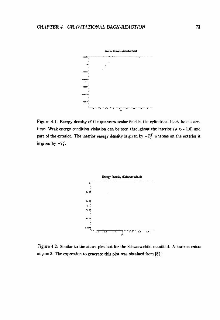
Figure 4.1: Energy density of the quantum scalar 6eld in the cylindrical black hole space-

time. CVeak energy condition violation can be seen throughout the interior ( p <- 1.6) and

part of the exterior. The interior energy density is given by -TT whereas on the exterior it

is giwn by -T;.

Figure 4.2: Similar to the above plot but for the Schwarzschild manifold. A horizon exists

at p = 2. The expression to generate this plot was obtained from [52].

of u and 17 yield:

where primes denote ordinary differentiation with respect to T. For the rest of this

chapter the dimensionless constant E will be set equal to one. It is also wvorth repeating

that the m a s term, hl is dimensionless as it is a m a s per unit length.

The metric components gn and 933 are not perturbed as it can be shown by

ut ilizing the Bianchi identities and the conservation law (covariant derivat ives taken

with respect to the background rnetric (1.33) ) that if (4.13a) and (4.13b) are solveri

then both equalities in (4.13~) must also be satisfied. -41~0, the eqiiality G$ = G\ via

(4.9) sets strict restrictions on the form of these perturbations and the only solutions

that may be found for the entire systern of equations are those where g ~ l and g3:~

remain unperturbed.

L'tilizing the above, the following solutions are obtained for the perturbations:

whereas the equation for a(T) yields:

& + - @ i 3 a ~ atan - - 3û3T3

480n [ 3 ( 2 1 l 3 + l)] + L6On ( 4 l l - û3T3) (AI + 3)

K(T) is a function whose derivative is known from (4.13a) and cancels al1 diver-

gences in a(T) (It can be shown, by solving the field equations near the horizon,

that o(T) is finite there). The actual form of this function is not important as only

derivatives of u(T) will be needed. The integration constant ko may be left arbitrary

as it does not enter subsequent caiculations. Both solutions are well behaved in the

domain of validity as ( p H ) = -& and o(ps) = 153-72 ln(3)-96 In(2)+-18 ln(bl)+l6\/3x 2 L6Or

Attention is now turned to the effects of the quantum perturbation on the

black hole spacetime. It has long been tbught that quantum effects may remove the

singular behaviour of physical spacetimes. Although the perturbative scheme can not

determine whether or not the actual singularity is removed, it can give information

on the growth of ciirvature scalars on the interior spacetime. Using the perturbed

metric, the Kretschrnann scalar can now be written as:

where Gi, is the unperturbed value given by (1.34) and SK is the first order cor-

rection term. CVhether or not cuntature is strengthened depends on the sign of 6K. If it is positive, the initial curvature growth is strengthened. If it is negatiw, it is

weakened.

The correction term is calculated to be

Although this result is extremely complicated when the solutions are substitu ted in,

a few relevant properties may be obtained. The value of BK near the horizon behaves

as

so that the limiting value at T = p~ is given by 6 K ( p H ) = &$. €rom which

it can be seen that cuwature groivth is strengthened at the horizon. The function

(4.18) increases as one passes through the horizon towards the singularity. Near the

singularity the curvature diverges as 1/TL6 although in this regime the approximation

breaks down and the expression has no physical meaning. At spatial infinity the

perturbation does not vanish due to the non vanishing nature of (T:) in anti-deSitter

spacetime so that 6K z and curvature is initially weakened.

For the case of Schwarzschild geometry the curvature perturbation diverges

as 1/P near the singularity for massless conformally coupled scalars 193) and in the

regirne where the perturbation is valid, curvature invariants are always strengthened.

At the event horizon of a Schwarzschild black hole, for example, the perturbation is

4.3 Summary

The stress energy tensor for a conformally coupled quantum scalar field has been cd-

culated in the black string spacetime and it is found that, as is cornmon with quantum

fields in curved spacetime, there exist regions where the weak energy condition is vio-

lated. The violation occurs on the interior and near the horizon on the exterior of the

black hole. From the stress energy tensor, the back-reaction has been calculated in the

form of the perturbed metric and Kretschmann scalar. Similar to the case of spherical

symmetry wit horit cosmological constant, it is found that curvature is strengthened

on the interior indicating that quantum effects in black holes may be geometry and

cosmological constant independent. Far away from the horizon fp » pH) , curvature

wvas found to be wveakened.

Chapter 5

Higher Derivat ive S tress-Energy

Tensors

The method of successive boundary counter-terms discussed in the introduction

is utilized here to render the asymptotically anti-de Sitter action finite. The equation

of motion derived from this action is then utilized to calculate conserved quantities

of various spacetimes of interest and both static and stationary cases are considered.

Results here may also be found in 11211. Recall from the discussion in the introduction,

this method was inspired from the Brown and York background subtraction technique

1361 where a quasilocal stress-energy tensor to be identified with the spacetime is

defined by:

with y,, being the rnetric of the r =fixeci surface for some large value of r . Although

(5.1) diverges as the boundary is taken to infinity, the stress-energy tensor is made

finite by subtracting a similar tensor defined on a reference or "background" spacetime.

Both the background subtraction and the boundary counter-term techniques are useful

as there elcists no asymptotically flat limit from which to define certain constants in an

asymptotcally AdS metric. The latter technique, studied here, has the advantage that,

via the .4dS/CFT correspondence, the resulting tensor should possess the properties

of the expectation value of a stress-energy tensor of a conformal quantum field theory.

At this point it is useful to recall From the introduction that in both schemes, the

CH4PTER 5. HlGHER DERNATIVE STRESS-ENERGY TENSORS 79

unrenormalised stress-energy tensor is given by

The motivation here is that such studies will shed light both in the gravitational sector

as well as the QFT sector of the theory. With this in mind the trace or Weyl anomaly

of the duai field theory is calculated at the end of the chapter.

To calculate the conserved charges, it is useful to write the line element of the

asymptotic AdS boundary in ADM form where the hypersurfaces (C) are spacelike

surfaces of constant t:

then the energy of the spacetime is obtained from the energy density as

where .ua is the unit normal to C and defines the local flow of time at the boundary.

In the =\DM formalism, a general conserved charge may be deterrnined via:

with < being the Killing vector generating the conserved current at the boundary.

To clarify the goal of this scheme and solidify what is meant by %nite con-

served quantities" consider the simple esample of Poincaré patch of .US3. This may

be written as:

The estrinsic curvature may be calculated via:

Nith unit normal to the T =Ld boundary

Applying (1.99) yields the following %nrenormalized" stress-energy tensor:

The mass may now be calculated using (5.4) yielding

which diverges as T" as the boundary is taken to infinity The finite, renormaiized,

energy must be independent of r and the counter-term technique is used here to make

such conserved quantities finite.

Although the pcimary interest here is in energies, other conserved quantities

may be similarly calculated by exploiting other Killing symmetries. The integral in

(5.4) d l diverge due to the asymptotic behaviour of the metric determinant unless

Tob(linitc) tends to zero for large r in such a way as to remove divergences. It is this requirement for the conserved quantities to be finite which uniquely determines the

form of the counter-terrns.

5.1 Calculat ions

Setting S(ct) = Ja, J i y i ~ ( ~ ~ ) the following Lagrangian is required to remove di-

vergences up to d=8 (631:

Note that this Lagrangian is similar to those considered in higher derivative gravity.

In fact, although the bu& theory is Einstein gravity, the boundary tbeory possesses

a higher derivative structure.

CHAPTER 5. HlGHER DERiV.4TM3 STRESSENERGY TENSORS 81

The action given by (5.11) is to be varieci with respect to the boundary metric, - 6S(ct', and this yields the following for the stress-eoeigy munter-term: 6706

b a .c 1 - (R' ' ):;] + (R@R*) , - - ( I P ~ R ~ ) ; , + (lr&yb 2 1

with Cab being the Einstein tensor fomed from the boundary metric This,

albeit rather large, expression will allow us to compute the conserved charges of the

spacetime '. Higher dimensional Schwarzschild-anti-deSitter black holes are chosen

'For calculations of conserved charges and Casimir energies of d = 4 Kerr-AdS spacetimes see

P221

as the systems of study whose geometry in Schwarzschild coordinates is given by:

where dQ; is the metric on unit d - 1-spheres which, for arbitrary p, is given by:

It should be noted that in the prescription employed here d l divergences are removed

by utilizing boundary terms. That is, only quantities intrinsic to the boundary are

subtracted. Therefore, quantities which are extrinsic to the boundary should only

appear at a finite level as nny extrinsic divergences can not be subtracted off. The

mass parameter, rg in (5.13) is an example of such a quantity and therefore this

appears only at the finite order and not in the counter-term.

Using (0.4) the masses of 7 and 9 dimensional black holes are calculated as

Follows (the mass of the five dimensional black hole has beeii previously calculated

in [621): First, the stress-energy tensor is calculated for the particular dimension of

interest by calculating both the unrenormalised stress tensor (5.2) and the counter-

term tensor given by (5.12). It is irnperative that the calculation of the counter-term

be tnincated at the correct order in a. That is, the first term in (5.12) is the only

term necessary for the case d = '2, the first two terms are required for d = 4 and so

on. Second, the renormalisation procedure is carried out by sirnply adding (5.2) to

(5.12). The rnass may now be calculated using (5.4) will be explicitly shown next for

the five dimensional Schwarzschild-AdS black hole.

Consider the metric for the 7 dimensional Schwarzschild-.4dS black hole,

This metric possesses lapse function

CH.4PTER 5. HIGHER DERNATIVE STRESSEWRGY TENSORS 83

as well as subspace volume element of

with

being the volume of pspheres. The local flow, um, is given by the normaliseci time-like

killing vector:

Utilising the above dong with (5.4) gives the expression for the m a s of the 7- dimensional black hole in the large r limit:

The procedure just described yields the following stress-eiiergy tensors and

masses for 7 and 9 dimensional black holes:

leading to (the five dimensional mass is given here as weI1)

In the limit of vanishing black hole mass, ro = O, there exists a pure vacuum state

which has non-zero energy. It was noted in 1621 and 11201 that, in light of the AdSJCFT correspondence 1331, the second term in 12[5 may be interpreted as the Casimir energy

of the dual field theory which k d = 4, N = 4, SUSY Yang Mills theory. It is

interesting to note that in seven dimensions the dual field theory has negative energy

whereas the other cases yield positive energy, The dual field theory to AdS7 x S4 supergravity is the large N limit of the d = 6 (2,O) tenmr multiplet theory 1331 of

which little is known. The field spectrum of this theory includes five scalars, two

Majorana-Weyl spinors and a 2-form potential, B, with self-dual three form field

strength, dB and is the intrinsic theory on iV parallel hi5 branes in the zero coupling

limit. The calculation here seems to imply that the Casimir energy of such a theory

on S5 x R is negative. The above expression may be converted to gauge theoretic

quantities via

with I, being the Planck length. This yields a Casimir m a s of

Examples of negative energy solutions in general relativity arc known such as

the analytically continued Reissner-Nordstrom solution (continued to both iniaginary

time and charge) although it is debatable how physical this construction is. Also,

it has been noted that if one considers the Euclidean time extension of D = d + 1

dimensional Schwarzschild-anti-deSitter black holes, the energy corresponding to the

dual gauge theory on Sd-l x SL is given by 1651:

where is the period of S' required to make the solution smooth at the (Euclidean)

horizon. The negative sign arises from the supersymmetry breaking boundary condi-

tions imposed dong S L . Since no such condition is imposed here in the D = 7 case

where the boundary topotogy is S5 x R it is curious that a negative energy is pro-

duced. This negative sign has the implication that the compact "boundary" spacetime

is more stable that the non-compact case for six dimensions.

It is also instructive to study spacetimes possessing non-zero angular momen-

turn.. Aside--Frorn the astrophysicalIy interesting applications to such spacetirnes it

CHAPTER 5. HIGHER DERNATIVE STRESSENERGY TENSORS 85

will extend the current calculations to other conserved quantities, specifically angular

momentum. The Kerr-AdS class of black hotes will be studied with the attention here

restricted to the one parameter class:

P2 d d i 2 = - - ( d t - sin2 B d 4 ) + -dr2 + -dB2 d - - A, Ae

with

The general properties of such solutions have been discussed in the introduction.

The counter-term technique is applied here to the d = 6 solution and is used

to calculate both the mass and angular momentum of the system. The latter quantity

is given by (in the =\DM formalism)

P. = J ~ o ~ ~ u , T ~ , (5.28)

with the subscript a representing an angular direction characterizing the angular

momentum. This calculation will aiso serve to shed light on whether or not the

negative Casimir energy survives when the dual field theory is defined on a rotating

universe which is the case for the boundary of rotating black holes. The d = 8 case

is intractable and therefore will not be considered. For d = 4 the calculation was

carried out utilising the background subtraction technique [391. The 11.1 = O iimit was

chosen as the reference spacetime for thuse caiculations. This corresponds to 4dS5 in a non-standard gauge. The background subtraction method does not, however,

produce vacuum contributions in the M + O IMit which are of some interest here.

For the conserved quantities of (5.26) both the Ttt and Tt4 components of the

stress-energv tensor will be needed. After a lengthy calculation, the following was

C W T E R 5. HIGHER D E W A T N E STRESS-ENERGY TENSORS 86

found for lowest order contribution to the m a s and angular momentum:

Hete, to avoid confusion in notation and make connection with the previous compu-

tations, the mass in (5.26) has been rewritten as ri/2. In the a + O limit, the mass is

identically that of (5.22b). The Casimir energy for the dual field theory to Kerr-AdS

should be defined as any contribution which is independent of the mass (1221. This

yields the following vacuum energy for the field theory defined on the boundary:

The presence of angular momentiim now gives the ground state a positive energy

contribution as can be seen in the third tetm of (0.30). However, there is no reat

value of a such that this yields a positive energy for (5.30).

5.1.1 Anomaly calculat ion

Recent interestitig work tegarding lower dimensional anornalies may be found in

Il231 and 11241 as well as Il251 where diffeomorphism techniques are utilized. Taking

the trace of the full stressenergy tensor yields:

The Weyl anomaly nust now be extracted from (5.31). To do this the metric

rnust be expanded in a power series in l l r ,

CHAPTER 5. HIGHER DEW.4TIVE STRESS-ENERGY TENSORS 87

(The Einstein equations, given below, dictate that no even power appears in the

expansion). This expansion allows the anomaly to be written in terrns of intrisic

curvature terms of the boundary by noting that the Einstein equations may be solved

order by order. This yields expressions for the Y[~)~~'s in terms of quantities intrinsic

to the boundary. The lowest order term in the e~pression (5.31) is then identified

with the anomaly.

Consider the Ad& metric

with extrinsic curvature of the boundary

This yiekls, for the three dimensional stress energy tensor's trace

Now the expansion (5.32) is utilisai which leads tu

By perturbatively solving the Einstein equations one finds

whcre R(o) is the Ricci scalar as a function of the boundary metric, g(0) only. Finally,

takiug the large T limit one finds:

which agrees with the trace anomaly of a 1 + 1 dimensional CFT [621. This scheme

has been shom to produce results in agreement with the work of Henningson and

Skenderis il261 for d 5 6. The d = 8 case is very labour intensive and will be addressed

utilizing a different rnethod to calculate the anomaly which is known to be consistent

mith the counter-term technique in lower dimensions.

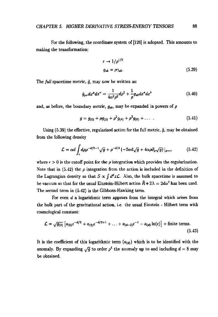
CHAPTER 5. HIGHER DEW4TIVE STRESS-ENERGY TENSORS 88

For the following, the coordinate systern of 11261 is adopted. This arnounts to

making the transformation:

The full spacetime metric, j , may now be written as:

and, as before, the boundary metric, gab, rnay be expanded in powers of p

üsing (5.39) the effective, regularized action for the full metric, ij, may be obtained

from the following density

wiiere é > O is the cutoff point for the p integration which provides the regularization.

Note tliat in (5.42) the p integration from the action is included in the definition of

the Lagrangian density so that S a d d x f . Also, the bulk spacetime is assumed to

be vacuum so that for the usiial Einstein-Hilbert action R + ~ A = 2da2 has been used. The second term in (5.42) is the GibbonsHarvking term.

For even d a logarithmic term appears from the integral which arises from

the bulk part of the gravitationai action, i.e. the usual Einstein - Hilbert term with

cosmological constant:

It is the coefficient of this logarithmic term (qd)) which is to be identified with the

anomaly. By expanding ,fi to order p" the anomaly up to and including d = 8 may

be obtained.

CHAPTER 5. HIGHER DERNATIVE STRESS-ENERGY TENSORS 89

The Einstein equations are given by 11261

where primes denote partial differentiation with respect to p and Tr is the trace

operator. Al1 quantities are constructed with respect to g.

The following relations between the g's may be determined by using equations (5.44c):

g(2)ab and g(41ab may be found in (1261 and are given here for reference.

CHAPTER 5. HIGHER DEW.4TZVE STRESS-ENERGY TENSORS 90

and gtj hm been calculated here by equating powers of p in (5.44a) and found to be:

where al1 covariant derivatives are now calcuiated with respect to g(o). 4s rnentioned

above, these expressions may be obtained €rom the Einstein equations and calculating

the Ricci tensor via (1.1) and (1.2). A11 partial derivatives are eliminated by rewriting

them as covariant derivatives minus the connexion and it is interesting to note that

al1 connexions cancel in the end leaving covariant derivatives only.

The expansion of g to order is needed to calculate the anomaly for d = 8. To this order:

where

2 - 1 3 -1 4 -1 -4 ~9&(2) + P g(qg(r) + P g(o~$(q + P g(o)~(s). (5.49)

The anomaly is now given by studying terms of O (p4) and using (5.45). In the process of calculating the d = 8 anomaly, the d = 2,4 and 6 were also calculated and

presented for completenm:

a(6) = a-5 [[f ( T ~ [g&(2i])3 - [g&(2)] Tr [(g6jg(2))*]

(5.52)

In general, up to constant coefficients, the anomaly to d dimension is given by al1 combinations of Tr.4 up to .id/?.

Curvature invariant terms, & which appear in the anomaiy are defined in

appendix 3. Since 96 may be replaced via (5.47) it is possible to calculate the anomaly

by utilizing (5.46a) and (5.46b) in (5.53). The resulting calculation is enormous. The

eight dimensional anornaly, as, is given by:

CH.4PTER 5. HIGHER DERNATIVE STRESS- ENERGY TENSORS 92

Note that, as with the lower dimensional cases, the anomaiy vanishes for Ricci flat

backgrounds.

5.2 Summary

-4 counter-term subtraction technique to study stress-energy tensors in higher

dimensional gravity was considered here. It is found that the counter-term method

consistently produces correct black hole masses for d 5 8 and therefore this is a

most useful technique even when there is no reference background with which to

renormalize the energy. The calculations also produce non-zero vacuum energies in

the ro = O limit. These may be interpreted as Casimir energies of the boundary

field theory (621 via the AdS/CFT correspondence which includes a negatiue energy

contribution for the (0,2) tensor multiplet theory dual to .4dSs. The Weyl anomaly

ntas also found by identifying logarithmic divergences in the gravitationai action.

Chapter 6

Conclusions

This thesis has utilized serni-classical techniques to study the back-reaction of

quantum fields on the singularity structure of a cylindrical black hole or black stririg

with cosmological constant. By studying the quantity (r$2), it was found that near

the horizon, vacuum polarization produces a maximum but finite value expectation

value. This study was then extended by calculating, in the one loop approximation,

the stress-energy tensor of the conformally coupled scalar field. Some exotic properties

were noticed such as energy condition violation near the horizon. The back-reaction

calculation revealed that although the curvature is weakened at spatial infinity (iinlike

the spherically syrnmetric, asymptoticaily fiat counterpart) the curvature near the

horizon was strengthened. This seerns to indicate that semi-classical effects near

black hole horizons (and perhaps the singularity although great care rnust be taken

when extrapolating to the singularity) are universal and independent of the spacetime.

It would be interesting to perform the same study in the Schwarzschild-de Sitter

or Schwarzschild-XdS spacetime. This would greatly aid the understanding of how

geornetry and cosmologicai constant affect the qualitative picture. In fact, future

work should most likely be directed towvards studying a generai class of black holes.

It should be possible to estend such studies to black holes of the form:

CHAPTER 6. CONCL USIONS

where

With this parameterization one may study a wide variety of black holes:

k = 1 corresponds to the spherical boundary (Reissner - Nordstrom black hole with

cosmological constant).

k = O corresponds to two cases: the torus (provided 19 and p are identified with certain

periods) and the cylinder.

k = -1 corresponds to the hyperbolic event horizon.

A slight modification to the above woulcl allow one to also study 'plana?' (domain

wall) black holes. It is also unclear at the moment how higher spin fields alter the

situation and an extension to spinors and vectors could be investigated. It should

be possible to study al1 these cases simultaneously and draw conclusions about how

quantum effects are afïected by geometry and field structure.

The gravitational stress-energy tensors in asymptotically AdS spacetimes were

also studied. These produced the correct mass for black hole spacetimes up to space-

time dimension D = 9. This tensor rnay also be used to study other properties of the

higher dimensional spacetimes such as angular momentum. This technique is iiseful

when exact solutions to the Einstein field equations are found that have unknown

constants which must be identified. These constants may unambiguously be associ-

ated with some conserved quantity by utilizing such boundary stress-energy tensors.

Another interesting property, via the AdS/CFT correspondence, is the ground state

or Casimir energy of the corresponding field theory. It is interesting that in the d = 6

case the minimal counter-term technique yields a negative Casimir energy for the dual

(0,2) tensor multiplet theory on Rx S5 boundary as well as the rotating 6 dimensional

Einstein universe. Although finite renormalizations can be utilized to set this energy

to zero, this addition of finite renormaiizations can be used in the other dimensions as

well and therefore does not expiain the discrepancy for this particular dimension. The

addition of angular momentum to the spacetime does not seem to alter the qualitative

picture.

CH.4PTER 6. CONCLUSIONS

Finally, the eight dimensional Weyl anomaly was calculated in terms of curva-

ture invariants. This quantity is not only useful for shedding some light on boundary

conformal field theories in this dimension but is also another step towards calculating

the anomaly in ten dimensions. This was one of the motivations in 1127) (who ana-

lyzed up to d = 6) as it would provide analysis of the quantum conforma1 structure of

ten dimensional field theories which are of central importance in theoretical physics

today. At the moment, extending calculations to higher dimension is intractable as

even in the d = 8 case the amount of algebraic manipulation is enormous, It is possi-

ble to deduce the types of terms which will appear in higher dimensional anomalies by

studying the progression (essentially how the Ki's evolve) as the riumber of dimensions

increases.

.As for the final fate of this work; 1 say to the binder "Bind this work quickly,

for the fire pit is ready and the cold weather conieth!"

Appendix A

World Function

In this appendix it will be demonstrated how to calculate the wvorld function,

O, using the method of geodesic expansion, Equations here involve quantities which

are defined at different spacetime points. For a brief review of handling bitensors the

reader is referred to Christensen 1461 and Synge 1471.

Let PL(x) that they are

and P?(x') be twvo points in the spacetime close enough together such

connected by a unique geodesic. The geodesic equation

yields the powr series 1

x p t; x"' + CJpl d s - - I ' $ c ~ a ~ a d s Z + 1 (2r$ , ï$ , ( i"(rU6) ds3 2 6

1 - G r ~ : d , , , ~ K ~ ~ d s 3 + ... (-4.2)

w here

and

The last term in equation (A.2) is zero since the spacetime is static. (A.2) can be

inverteci and used in the definition 1471

2o(x, x') = ds2 gP~,,d~J (A.5)

APPENDLY A. WORLD FUNCTlON

giving

Calculating the Christoffel symbols using (1.33) and noting (A.4) it can be shown that

this expression reduces to the one in (3.17). This expression has the same functional

form as that of the world function for a static, spherically symmetric spacetime 1831

if the coordinate separation there is also chmen as (A.4). This is due to the fact that

the <p vectors eliminate any dependence of a(z, x') on g22 and 933.

Appendix B

Horizon Value of ($2)

In this appendix the dominant terms of (#*) at the horizon will be calculated

from the WKB approximation. This is useful since the value at the horizon ne&

to be evaluated as a starting point for the calculation of the mode functions. This

calculation is also useful as it provides insight as to how the n counter-term acts to

regdarise the field.

At the horizon, the dominant tenns in the field expansion are given by

where h was defined in (3.30). For the moment, Ive choose to ignore the 1 = O term

and concentrate on the first expression in (B.1) which can trivially be re-written as

APPENDIX B. HORIZON VALUE OF (42) 99

The product in the above expression is well known yielding the following for (B.2)

For very large n or (as in the case here) very small h this becomes

If we define the 1 = O term to cancel out the second term in (B.3) the resultant

expression gives

which is cancelled by the n sum in the counter-term. This leaves a small constant

contribution to (q5*) at the horizon.

Appendix C

Linearly Independent Ki

The linearly independerit curvature invariants which appear in the calculaticin of

the eight dimensional Weyl anomaly are tabulated here for convenience. The notation here follows that of 11-71.

K L = Rk' Rlm Rms RSk,

h3 = R~ RrnnR,,,,,,

h'j = ( R ~ " & , ) ~ ,

Ki = Rn' Rlm Dp Dn R"",

K~ = R ~ ~ R ~ , D"D,R,

Kll = RRmnDm DnR,

KL3 = i i20R,

Icl.5 = (DmDnR) (ORmn) 7

K1i = ( D p D n E ) (DmDnR) ,

h*19 = Rmn Rm Dp Dn R,

= R ~ J D ~ D ~ D " DkR7

= RkiDbDj (OR)

b.5 = RDnDmORnm,

K27 = R ~ ~ D , D ~ D , D ~ R ,

K2 = RRkm RmS R:

K4 = RJ 4 = R~~ R~~~~ R ~ R , , ~ ~

& = RRmn DP

=

K12 = R R m n O k n

KL4 = (DmDnR) (DnDmR)

KL6 = ( 0 ~ ) ~

Kl8 = ( O h m ) (ORmn)

K20 = Rmn&nOR

K22 = Rk'DnDjO~;

= R D ~ D ~ D ~ D ~ R

K% = RO (OR)

K2* = Rmno

K29 = (DpDnR;) (ORmn) 9

K3, = RmnRpqDmDnRpql

Km = Rrn" RD, Dn R,

K35 = RmnRPqm,DpDnF,

K31= Rmn ( D p p ) ( & R h r ) K 3 g = Rmn ( P , RP9) (DpRgm) ,

fii = RmnRWDpDmRq,

K3 = Rmn (Dp R) (Dn RP,) ,

&S = R (DmRnp) (Dqflnmp) , h;7 = R (DmRnP) (Dn&)

&g = Rmn (DcRW) (DCR,,,,,)

= RmnRPnDR,,,p,

K ~ J = Rmn (DcR) ( D E R , , ) ,

h'js = RmnO (Dm Dn R) ,

Bibliography

fll Lemos, J. P. S. and Zanchin, V. T. Phys. Reu. D. 54 (1996), 3840.

121 Misner, C. W., Thorne, K. S. and FVheeler, J. A. Cmvitation. New York: Freernan,

1973.

131 Thorne, K. S. Black Holes & Time Warps: Einstein's Outrageous Legacy. Xew York:

Norton, 1994.

[4f Hawking, S. W. and Ellis, G. F. R. The Large Scale Structure of Spce-time. Cambridge:

Cambridge, 1973.

1.51 Einstein, A. Ann. Math. 40 (1939), 922.

[6] Schwarzschild, K. Sitz. Deutsch. Akad. Wis. (1916), 189.

[7] Oppenheimer, J. R. and Snyder, H. Phys. Reu. 56 (1939), 455.

[8] May, M. M. and White, R. H. Bul. Am. Phys. Soc. 10 (1965), 15 and Phys. Reu. 141

(l965), 1232.

19) Podurets, M. A. Dok. Akad. Nuuk. 154 (1964), 300 or English translation Sou. Phys.

-Dok. 9 (1964), 1.

[101 Penrose, R. Phys. Rev. Let. 14 (1965), 57.

[Ill Geroch, R. P. Ann. Phys. 48 (19681, 526.

[121 Schmidt, B. G. Cen. Rel. Gmv. 1 (1971), 269.

1131 Wdd, R. Cenenil Relativz'ty, Chicago: University of Chicago, 1984.

[14] Levi-Civita, T. Rend. Acc. Lincei. 26 (1917), 317

[15] Curzon, B. E. J. Proc. R. Soc. Lmdon. 23 (1924), 477.

[16] Chazy, J. Bull. Soc. Math. h n c e 52 (19241, 17.

[171 Weyl, H. Annalen Phys. 54 (1917), 117.

[181 Lewis, T. Proc. R. Soc. London A136 (1932), 176.

[191 Kaloper, N. Phys. Reu. D 48 (1993), 4658.

1201 Shapiro, S. L. and Teukolsky, S. A. Phys. Reu. Lett. 66 (1991), 944.

[21I Kibble, T. W. B. J. Phys. 9 (1976), 1387.

[221 Magueijo, J. and Brandenberger, R. Invited Lectures at the International School on Cos-

rnology, Kish Islaiid, Iran. astro-ph/Oûû2030. To be published in Large Scale Structure

Formution, Kluwer, Dordrecht, 2000.

[231 Peebles, P. J. E. Princtples of Physical Cosmology, Priiiceton: Princeton University

Press, 1993.

[21j .Alexander, S. Ph.D. thesis and hep-th/9912037.

1251 Brandenberger, R. Invited Lectures ut the Intemolional School on Cosmology, Kish

Islaud, Iran. hep-ph/99104 10.

[26] Vishniac, E. T., Olive, K. A. and Seckel, D. Nucl. Phys. B289 (1987), 717

[27] Vilenkin, A., and Sheiiard: E. P. S. Cornac Strings and Other Topological Defecls. New

York: Cambridge, 1994.

[28] Hindmarsh, M. B. and KibbIe, T. W. B. Rept. Pmg. Phys. 58 (19951, 477.

f29j Avis, S. J., Isham, C. J. and Storey, D. Phys. Reu. D. 18 (1978), 3565.

f301 Lemos, J . P. S. Phys. Reu. D. 57 (1998), 4600.

1311 Smith, F i . L. and Mann, R. B. Phys. Reu. D. 56 (1997), 4942.

1321 Witten, E. Commun. Math. Phys. 80 (1981), 381.

[331 Maldacena, J. Adu. Thwr. Phys. 2 (1998), 231.

(341 Witten, E. Adu. Theor. Math. Phys. 2 (1998), 253.

[351 Baiiados, M., Teitelboim, C., and Zanelli, J. Phys. Rev. Let. 69 (1992), 1849.

[361 Brown, J. D., and York, J. W. Jr. Phys. Rev. D. 47 (1993), 1107.

[37l Vanzo, L. Phys. Rev. D. 56 (1997), 6475.

[381 Witten, E. Adu. Theor. Math. Phys. 2 (1998), 505.

[391 Hawking, S. W., Huater, C. J., and Taylor-Robinson, M. M. hep-th/9811056.

[401 Penrose, R. Rev. del Nuouo Cimento. 1 (1969), 252.

1411 DeWitt, B. S. Phys. Rpb. 6 (1975), 296.

[421 Birrell, N. D., and Davies, P. C. W. Quantum Fields in Curved Space. New York:

Cambridge, 1982.

[431 Wald, R. M. Quantum Field Theoy in Curved Spacetime and Black Hole Thermody-

namics. Chicago: University O€ Chicago Press, 1994.

1441 Wipf, -4. Quantum fields near black holes. hep-th 9801025 (1998).

[45l Hawking, S. W. Commun. Math. Phys. 43 (1975), 199.

[46j Christensen, S. M. Phys. Reu. D. 14 (1976), 2490.

[471 Synge, J. L. Relatiuity: The Generul Thwry. Amsterdam: North-Holland, 1964.

[481 Hadamard, J. Lectures on Cauchy's problem in Linear Partial Diffemntial Equations.

New Haven: Yale University Press, 1923.

[491 Van Vleck, J. H. P m . Nat. Acad. Sci. US. 14 (1928), 178.

(501 Uinkhammer, G . Phys. Rev. D. 43 (1991), 2542.

[51j Brown, L. S. and Cassidy, J. P- Phys. Rev. D. 16 (1977), 1712.

[521 Page, D. X. Phys. Reu. D. 25 (1982), 1499.

[531 Howard, K. and Candelas, P. Phys. Reu. Lett. 53 (1984), 403.

[541 Wald, R. M. Commun. Math Phys. 54 (1977), 1.

[551 Pilkey, D. Big Dog and Little D g Cetling into ïkouble. San Diego: Harcourt Brace and

Co., 1997.

[56l Duff, M. J. Nucl. Phys. B125 (1977), 334.

[571 Simon, J. 2. Phys. Rev. D. 45 (1992), 1953.

[591 Einstein, A. Sitz. Preuss. Akad. Wiss. (1916), 696.

[601 Levi-Civita, T. Rendiconti della Reale Accademia dei Lincei. 26 (1917), 381.

Or see translation: Antoci, S. and Loinger, A. physics/9906004.

[611 Babak, S. V. and Grishchuck, L. P. gr-qc/9907027,

[621 Balasubrarnanian, V. and Kraus, P. hep-th/9902121.

[631 Kraus, P., Larsen, F. and Siebelink, R. hep-th/9906127.

[64 Emparan, R., Johnson, C. V. and Myers, R. C. Phys. Rev. D. 60 (1999), lM001.

[65l Horowitz, G. T. and Myers, R. C. Phys. Rev. il. 59 (1999), 026005.

1661 Fefferman, C., and Graham, C. R. Elie Cartan et les Mathematiques d'aujourdhui.

Asterisque, 1985, p95.

(671 Gubser, S. S., Klebanov, 1. R. and Polyakov, A. 51. Phys. Lett. B 428 (1998), 105.

[681 Bekenstein, J. D. Phys. Reu. D. 7 (1973), 2333.

[701 Gibbons, G . W. and Hawking, S. W. Phys. Rev. D. 15 (1977), 2738.

1711 Hawking, S. W. and Page, D. N. Commun. Math. Phys. 87 (1983), 577.

1721 Baïiados, M., Teitelboim, C. and Zaneiii, J. Phys. Rev. Lett. 69 (1992), 1849.

BlBLIOGR4 PHY

[73) Reznik, B. Phys. Rev. D. 51 (1995), 1728.

[741 Oda, 1. Phys. Lett. 409 (1997), 88.

[751 Brown, J . D., Creighton, J. and Mann, R. B. Phys. Rev. D. 50 (1994), 6394.

[76] Kaioper, BI. Phys. Rev. D. 48 (1993), 4658.

[771 Allen, B., Folacci, A. and Gibbons, G. W. Phys. Lett. B. 189 (1987), 304.

[78j Peca, C. S. and Lemos, J. P. S. gr-qc/9809029.

1791 DeBenedictis, .A. Gen. Ref. Cmv. 31 (1999), 1549.

1801 Hawking, S. W. Commun. Math. Phys. 80 (1981), 421.

1811 Candelas, P. and Howard, K. W. Phys. Rev. D. 29(1984), 1618.

1821 CandeIas, P. and Jensen, B. P. Phys. Rev. D. 33 (1986), 1596.

1831 Anderson. P. R. Phys. Rev. D. 41 (1990), 1152.

1841 .Anderson, P. R., Hiscock. W. .A. and Larson, D. .A. Phys. Rev. Lett. 70 (1993), 1739.

1851 ..\ntlerson, P. R., Hiscock, W. .A. and Larson, D. -4. Php. Rev. D. 51 (1995), -1337.

[861 Frolov, V. P. Quantum Cmvity, pmeedings of the second seminar on Quantum Gmvity,

Singapore: World Scientific, 1984, p 303.

[87j Frolov, V. P. and Thorne, K. S. Phys. Rev. D. 39 (1989), 2125.

[88] Frolov, V. P. and Zel'nikov, .A. 1. Phys. Rev. D. 29 (1984), 1057.

1891 Hiscock, IV. -4. and CVeems, L. Phys. Rev. D. 4 1 (1990), 1142.

[901 Bardeen, J. 51. Phys. Rev. Lett. 46 (1981), 382.

[911 Balbinot, R. Class. Quantum Gmv. 1 (1984), 573.

[921 York, J. W. Phys. Rev. D. 31 (1985), 775.

[931 Hiscock, W. A., Larson, S. L. and Anderson, P. R. Phys. Rev. D. 56 (1997), 3571.

BIBLIOG R4PHY

1941 Lifschytz, G. and Oritz, M. Phys. Reu. D. 49 (1994), 1929.

1951 Steif, .4. R. Phys. Reu. D. 49 (1994), 585.

[96j Shiraishi, K. and Maki, T . Class, Quantum Gmu. 11 (1994), 695.

[971 Mann, R. B. and Solodukhin, S. N. Phys. Reu. D. 55 (1997), 3622.

[981 Lemos, J . P. S. and Zanchin. V. T. Phys. Rev. D. 53 (19961, 4686.

1991 Witten, E. Adv. Thwr. Math. Phys. 2 (1998), 505.

(1001 Plana, .Y. Mem. della R. Accad. di Tomho. XXV (1820), 343.

[IO11 Brown, J. D., Creighton, J. and Mann, R. B. Phys. Rev. D. 50 (1994), 6394.

[IO21 DeBenedictis, A. Class. Quant. Grau. 16 (1999), 1955.

[IO31 Parker, L, and Fulling, S. Phys. Reu. D. 7 (1973), 2357.

[IO41 Starobinsky, A. A. Phys. Lett. 91B (1980), 99.

[IO51 Fischetti, 31. V., Hartle, J. B. and Hu, B. L. Phys. Reu. D. 20 (1979), 1737.

[IO61 Anderson, P. Phys. Reu. D. 28 (1983), 271.

[ loi] .huma, T. and Wada, S. Prog, Theor. Phys. 75 (1986), 845.

[IO81 Hartle, J. B. and Hawking, S. W. Phys. Reu. D. 13 (1976), 2188.

[IO91 Brandenberger, R., Mukhanov, V. and Sornborger, A. Phys. Reu. D. 48 (1993), 1629.

[Il01 Easson, D. A. and Brandenberger, R. H. JHEP. 09 (1999), 003.

[Il11 Anderson, P. R., Hiscock, W. A. and Loranz, D. 3. Phys. Rev. Lett. 74 (1995), 1365.

[Il21 Anderson, P. R., Hiscock, W. A. and Samuel, D. A. Phys. Reu. D. 51 (1995), 4337

[Il31 Frolov, V. P. Phys. Reu. D. 21 (1982), 2185.

[Il41 Zellnikov -4 I and Froiov V P 1987 Pmeedings of the Lekdev Physics Iwtitute of the

Academy of Sciences of the USSR. 169 New York: Nova Science, 1987, p171.

[Il51 Shiraishi, K. and Maki, T. Phys. Reu. D. 49 (1994), 5286.

[Il61 Shiraishi, K. and Maki, T. Class. QUanf. Gmv. 11 (1994), 1687.

[Il71 Mann, R. B. and Solodukhin, S. N. Phys. Rev. D. 55 (1997), 3622.

[Il81 Bekenstein, J. D. and Parker, L. Phys. Rev. D. 23 (1981), 2850.

[Il91 Brown, M. R.? Ottewill, A. C. and Page, D. N. Phys. Reu. D. 33 (1986), 28-LO.

[1201 M yen, R. C . hep-th/9903203.

[1211 DeBenedictis A. and Viswanathan K. S. hep-th/9911060.

(1221 Awad, A. M. and Jobnson, C. V. hep-th/9910040.

[1231 Nojiri, S . and Odintsov, S. D. hep-th/991 Ull3.

[1241 Ho, 3. hep-th/9910124.

il251 Imbimbo, C. , Schwimmer, A., Theisen, S. and Yankielowicz, S. hep-th/9910267.

[1261 Henningson, M. and Skenderis, K. hep-th/9812032 and Henningson, M. and Sk- enderis, K. J . High Energy Phys. 07 (1998), 023.

[1271 Bonora, L., Pasti, P. and Bregola, M. Chs. Quant. Gmv. 3 (1986), 635.

GEOMETRODYNAMICS OF QUANTUM FIELDS IN BLACK HOLE ANTI-DE SITTER

Documents

Transcript of GEOMETRODYNAMICS OF QUANTUM FIELDS IN BLACK HOLE ANTI-DE SITTER