
GEOMETRICALLY DECOUPLED PHASED ARRAY COILS FOR...
88
GEOMETRICALLY DECOUPLED PHASED ARRAY COILS FOR MOUSE IMAGING A Thesis by SAHIL BHATIA Submitted to the Office of Graduate Studies of Texas A&M University in partial fulfillment of the requirements for the degree of MASTER OF SCIENCE May 2009 Major Subject: Biomedical Engineering
Transcript of GEOMETRICALLY DECOUPLED PHASED ARRAY COILS FOR...

GEOMETRICALLY DECOUPLED PHASED ARRAY COILS FOR MOUSE
IMAGING
A Thesis
by
SAHIL BHATIA
Submitted to the Office of Graduate Studies of Texas A&M University
in partial fulfillment of the requirements for the degree of
MASTER OF SCIENCE
May 2009
Major Subject: Biomedical Engineering

GEOMETRICALLY DECOUPLED PHASED ARRAY COILS FOR MOUSE
IMAGING
A Thesis
by
SAHIL BHATIA
Submitted to the Office of Graduate Studies of Texas A&M University
in partial fulfillment of the requirements for the degree of
MASTER OF SCIENCE
Approved by:
Chair of Committee, Mary P. McDougall Committee Members, Steven M. Wright Jim X. Ji Head of Department, Gerard L. Cote’
May 2009
Major Subject: Biomedical Engineering

iii
ABSTRACT
Geometrically Decoupled Phased Array Coils For Mouse Imaging. (May 2009)
Sahil Bhatia, B.E., Thadomal Shahni Engineering College, Mumbai
Chair of Advisory Committee: Dr. Mary P. McDougall
Phased array surface coils offer high SNR over a large field of view. Phased array
volume coils have high SNR at the surface and centre of the volume. Most array coil
designs typically employ a combination of geometrical and additional techniques, such
as isolating preamplifiers for element-to-element decoupling. The development of array
coils for small animal MRI is of increasing interest. However isolation preamplifiers are
expensive and not ubiquitous at the field strengths typically employed for small animal
work (4.7T, 9.4T, etc). In addition, isolating preamps complicates the designs of coils for
transmit SENSE since they do not decouple during transmitting. Therefore, this thesis
reexamines a “tried and true” method for decoupling coil elements. In this work five
different coils for mouse imaging at 200MHz are presented: a 16 leg trombone design
quadrature birdcage coil and four geometrically decoupled volume phased array coils.
The first mouse array coil is a two saddle quadrature coil with a circularly polarized
field. The second coil is a four channel transmit/receive volume array coil that is
decoupled purely geometrically, without the need for other forms of decoupling. The
third array coil is a modified ‘open’ configuration to facilitate the loading of animals.
The fourth coil presented is a ‘tunable’ decoupling coil, where the geometric decoupling

iv
between elements is ‘tunable’, in order to compensate for different loading conditions of
the coil.
Tunable decoupling between elements was achieved using two mechanisms, a
decoupling paddle for isolation of top to bottom elements, with a variable overlap
mechanism for decoupling diagonal elements. Bench measurements demonstrate good
decoupling (better than -20dB) of the coil elements and ‘tunability’ of both mechanisms.
Phantom images from all coils are presented.

v
DEDICATION
I would like to dedicate this thesis to my “Daadu” (grandmother), Mrs. Krishna Bhatia.
At age 85, no wait.. . At age 25 she is as fit as people half her age and a source of
inspiration for me. A mother of six, grandmother of twelve and a great grandmother of
two children and many more to come, she has taken care of each one of us with lots of
love and affection. It is her support that has taken me through many tough times in life.
This is just a small way for me to say Thank You “Daadu”. I hope I keep making you
proud!
म यह थसस अनी दाद मत ा भातया को अपत कना चाहगा. ८५ साल क उमर, मरा म%लब ह
२५ साल क उमर मई इ*ी द,-त ह वोह क उस आधी उमर क लोग शमा जाय. उहोन अन ६ ब4चो,
१२ पोत/पोतयोन को, और २ नातयो को बहत सारा यार और आशवाद 7दया ह. ऊक 9ो%साहन क:
वजह स ह; म अनी िजदगी मइ आग ब= पाया हन. म आशा करता हन क म ऐस ह; आग जाक काम
क? िज-स आको म@पर गव हो. थक योउ दाद!

vi
ACKNOWLEDGEMENTS
I would like to thank my committee chair, Dr. McDougall, and my committee members,
Dr. Wright and Dr. Ji, for their guidance and support throughout the course of this
research.
Big thanks to my friends at MRSL John Bosshard ,Cheih Wei Chang, James Chen,
Arash Dabirzadeh, Neal Hollingsworth, Ke Feng, Vishal Kampani, Katie Ramirez, Bijay
Shah and Naresh Yallapragada. Thanks guys for sharing your know-how and
knowledge. I appreciate the patience that you all showed to answer all my stupid
questions.
I am grateful to Dr. Fraser Robb for giving me an opportunity to work at G.E. Healthcare
with some of the brightest minds and nicest people I’ve met. Thanks Yiping Guan, for
the ideas and guiding me during this research. It was a pleasure working with a person
with your knowledge and experience.
Finally, thanks to my father, mother, sister and grandmother for their constant
encouragement, love and support.

vii
NOMENCLATURE
RF Radio Frequency
GE General Electric
C1 Coil 1 – Trombone design quadrature birdcage coil
C2 Coil 2 – Two saddle quadrature coil
C3 Coil 3 – Four channel array coil
C4 Coil 4 – Four channel ‘open’ array coil
C5 Coil 5 – Four channel ‘tunable’ decoupling array coil

viii
TABLE OF CONTENTS
Page
ABSTRACT .............................................................................................................. iii
DEDICATION ........................................................................................................... v
ACKNOWLEDGEMENTS ....................................................................................... vi
NOMENCLATURE .................................................................................................. vii
TABLE OF CONTENTS .......................................................................................... viii
LIST OF FIGURES ................................................................................................... x
LIST OF TABLES ..................................................................................................... xiii
1. INTRODUCTION ............................................................................................... 1
2. THEORY ............................................................................................................. 4
2.1 Magnetic Resonance Imaging .............................................................. 4 2.2 Birdcage coils ....................................................................................... 7 2.2 Circularly polarized field ...................................................................... 10 2.3 Surface coils ......................................................................................... 13 2.4 Phased array coils ................................................................................. 14 3. MATERIALS AND METHODS ........................................................................ 18
3.1 Circularly polarized trombone design birdcage coil (C1) .................... 18 3.2 Two saddle quadrature coil (C2) .......................................................... 21 3.3 Four channel array coil (C3) ................................................................. 22 3.4 Four channel ‘open’ array coil (C4) ..................................................... 23 3.5 Four channel ‘tunable’ decoupling array coil (C5)............................... 24 3.6 Supplementary apparatus ..................................................................... 28 4. RESULTS ............................................................................................................ 32
5. DISCUSSION ....................................................................................................... 46
6. CONCLUSION .................................................................................................... 56

ix
Page
REFERENCES .......................................................................................................... 58
APPENDIX ............................................................................................................... 62
VITA .......................................................................................................................... 75

x
LIST OF FIGURES
FIGURE Page
1 A nucleus precessing about an applied magnetic field of strength B0 ........ 5
2 Schematic of 8 leg birdcage coils ............................................................... 8 3 Segment of equivalent circuit of a high pass birdcage coil ........................ 9 4 A circular surface coil. ................................................................................ 14 5 Single square coil resonating at frequency f0 ............................................. 15 6 Mutually coupled coils .............................................................................. 16 7 Mutually decoupled coils ............................................................................ 16 8 Phased array coil of four elements. ............................................................. 17
9 Circular endring of birdcage coil ................................................................ 19 10 Trombone design quadrature birdcage coil. ............................................... 20 11 Two saddle quadrature coil ......................................................................... 21 12 Four channel array coil ............................................................................... 22
13 CAD drawing of four channel ‘open’ array coil ......................................... 24 14 Four channel ‘open’ array coil ................................................................... 24 15 Showing the region of overlap .................................................................... 25
16 Old element shape and modified new element shape…………………….. 25
17 Four channel “tunable” decoupling array coil ........................................... 26
18 Electrical circuit of a single coil element and feedboard. ........................... 28
19 Centering mechanism attached to the birdcage coil ................................... 29

xi
FIGURE Page
20 Mechanism centering the array coils inside the detunable birdcage coil ... 30
21 Resolution structure .................................................................................... 31 22 T/R images of CuSO4 phantom ................................................................. 34 23 Images of CuSO4 phantom ........................................................................ 35 24 Coronal image of CuSO4 phantom ............................................................ 35 25 Coronal image of CuSO4 phantom ............................................................ 36 26 Processed axial images of CuSO4 phantom ............................................... 37 27 Processed transverse images of CuSO4 phantom ...................................... 37 28 Decoupling paddle at different overlap positions ....................................... 38 29 Graph of S21 vs. paddle position ................................................................. 39
30 Graph of S34 vs. paddle position ................................................................. 40
31 Showing different positions of overlap ...................................................... 41
32 Graph of S32 vs. overlap length ................................................................. 42
33 Graph of S31 vs. overlap length. ................................................................. 43 34 Graph of S41 vs. overlap length ................................................................. 44
35 Graph of S42 vs. overlap length .................................................................. 45
36 Axial images of a mouse passing through its heart………………………. 45 37 Images with other loops terminated to 50Ω……………………………… 47 38 Images with other loops open circuited………………………………….. 48 39 Images with coil closed…………………………………………………... 48 40 Images with coil open……………………………………………………... 49

xii
FIGURE Page
41 Coronal Images………………………………………………………….... 49 42 Magnitude and phase plots of full FOV images…………………………... 50 43 Full FOV g factor map..…………………………………………………... 51 44 Magnitude and phase plots of reduced FOV images…….……………….... 52 45 Reduced FOV g factor maps……………………………………………… 52 46 Showing S21 [dB] measurements with flux probe…………...……….. ..... 54 47 Circuit showing position of the tuning and matching capacitors .............. 70
48 Central core and shield of the semi rigid cable…………………………. 72
49 Stepwise construction of a balun………...……….. ................................... 72
50 Showing the two ends of a fabricated balun…………...……….. .............. 73

xiii
LIST OF TABLES
TABLE Page 1 Five RF coils designed and fabricated for mouse MRI…………………… 18 2 S Matrix [dB] for trombone design quadrature birdcage coil C1 ............... 31 3 S Matrix [dB] for two saddle coil C2…………………………………………... 32
4 Matrix showing coupling [dB] for coil C3……………………………………. 32 5 Matrix showing coupling [dB] for coil C4 ................................................. 32
6 S21 values at different positions of the paddle for two loads…………………. 37 7 S34 values at different positions of the paddle for two loads……………… 38 8 S32 values at different positions of the paddle for two loads……………. 40 9 S31 values at different positions of the paddle for two loads……………. 41 10 S41 values at different positions of the paddle for two loads……………… 42 11 S42 values at different positions of the paddle for two loads……………. 43

1
____________ This thesis follows the style of Concepts in Magnetic Resonance Part B (Magnetic Resonance Engineering).
1. INTRODUCTION
In 1990 Roemer et al [1] introduced phased array surface coils. Localized surface coils
provide high SNR from a region that is limited to the dimensions of the surface coil.
Roemer’s phased array, then, comprised of multiple surface coils, offered high SNR in
an MR image over a large field of view. Nearest neighbors in an array can be decoupled
by overlapping adjacent elements while low input impedance preamplifiers are often
used, and are in fact depended upon to decouple next nearest neighboring elements.
When using phased array coils, it has become common to connect each of these coils to
a separate preamplifier and receive channel. Phased array volume coils were introduced
soon after by Hayes et al [2]. These had high SNR at the surface of the volume and also
high SNR at the centre. Since then, phased array coils have become standard in clinical
MR imaging.
Phased array coils are gradually moving into the field of small animal research. Recently
specialized phased array coils with as many as 20 channels have been developed for
mouse imaging at 3 T [4]. At 4.7 T four-channel receive-only phased-array coils show
images of cats and mice [5, 6], while there is ongoing development of building a
superconducting 2 element array [7]. An important factor in designing of phased array
coils is the decoupling of coil elements. Commonly, geometrical decoupling is used to
decouple nearest neighbors while preamp decoupling to decouple next nearest neighbors

2
as shown in the 4 element array built by Gareis et al [8]. When using preamplifier
decoupling, a deactivation circuit is formed by a parallel capacitor and a series inductor.
At the desired frequency this circuit provides high impedance which open circuits the
receive coil. There is no flow of current in the coil hence coupling is reduced to
minimum whereas the coil still faithfully transfers the NMR signal to the preamps.
Techniques such as transformers decoupling [9] and capacitive decoupling have also
been shown in mouse coils [10]. Simulation studies [11] and specialized transmit-receive
coils of up to 4 channels have been shown at 9.4T and ultra high field strengths of 17.6T.
Most array coil designs typically employ a combination of techniques such as geometric,
capacitive, transformer and preamplifier decoupling techniques for element-to-element
decoupling. However isolation preamplifiers are expensive and not ubiquitous at the
field strengths typically employed for small animal work (4.7T, 9.4T, etc). In addition,
isolating preamps complicate the designs of coils for transmit SENSE since they do not
decouple during transmit. Therefore, we have re-examined a “tried and true” method for
decoupling.
In this work we have examined volume coils for mouse imaging. This includes phased
array coils that are decoupled purely geometrically, with modifications to create an
‘open’ configuration coil to facilitate the loading of animals and a configuration with
‘tunable’ decoupling of elements. We describe here the design and construction of these
coils for imaging at 4.7T (200MHz). Tunable decoupling between elements was

3
achieved using two different mechanisms: a decoupling paddle for isolation of top to
bottom elements, while a variable overlap mechanism for decoupling diagonal elements.
Bench measurements show good ‘tunability’ of both mechanisms – i.e. the mechanisms
can optimize decoupling of the overlapping elements over a range of loading conditions,
avoiding the tedious soldering and desoldering processes involved with optimizing the
decoupling between overlapping elements.

4
2. THEORY
2.1 Magnetic Resonance Imaging
Magnetic Resonance Imaging (MRI) is a powerful imaging technique. Nuclei that have
an odd number of protons, neutrons or both can be used in MRI imaging. The most
common nucleus studied is the hydrogen proton, due to its high abundance in the human
body. In Magnetic Resonance Imaging (MRI) the sample to be imaged is placed in a
uniform magnetic field, the equilibrium magnetization vector is displaced with a pulse at
Larmor frequency, and the signal that is obtained as the magnetization vector returns to
equilibrium is observed.
The motion of the hydrogen proton around the centre of the nucleus is known as orbital
motion. The proton also rotates (spins) about its own axis, the motion about its axis is
also known as spinning. Both these motions have an associated angular momentum. In a
stable state the angular momentum of paired neutrons or protons are in the opposite
direction i.e., the protons arrange themselves in a ‘spin pairing’ state (spin up and spin
down). The hydrogen proton also has an associated Magnetic Dipole Moment (MDM).
MDM is associated with the motions of the charged proton. The MDM is a characteristic
of an element which indicates how fast the protons align themselves along an external
magnetic field.

The axes of the protons are initiall
magnetic field they try to align their
protons can only align themselves at an angle with respect to the magnetic field. Protons
align themselves in either of two orientations along the field. The up orientation or spin
up state has lower energy and makes an angle θ with the field. The down orientation or
spin down state has higher energy and makes an angle 180
protons are not perfectly aligned with the magnetic field they still have some resultant
torque. This results in the protons spinning about the magnetic field as shown in Figure
1. This spinning motion is called precession.
Figure 1: A nucleus precessing about an applied magnetic field of strength B
The frequency at which the nucleus precesses is called Larmor frequency. The Larmor
frequency is given by,
where is Larmor frequency, γ=gyromagnetic ratio, B
The ratio of MDM and the spin angular momentum is called Gyromagnetic Ratio and it
is given by,
The axes of the protons are initially randomly oriented, but when placed in an
y try to align their axes along the field. Due to quantum rules, the
protons can only align themselves at an angle with respect to the magnetic field. Protons
of two orientations along the field. The up orientation or spin
up state has lower energy and makes an angle θ with the field. The down orientation or
spin down state has higher energy and makes an angle 180- θ with the field
ctly aligned with the magnetic field they still have some resultant
torque. This results in the protons spinning about the magnetic field as shown in Figure
1. This spinning motion is called precession.
nucleus precessing about an applied magnetic field of strength B
The frequency at which the nucleus precesses is called Larmor frequency. The Larmor
VL = γ·B0 / 2·π
where is Larmor frequency, γ=gyromagnetic ratio, B0=Magnetic field.
The ratio of MDM and the spin angular momentum is called Gyromagnetic Ratio and it
5
y randomly oriented, but when placed in an external
axes along the field. Due to quantum rules, the
protons can only align themselves at an angle with respect to the magnetic field. Protons
of two orientations along the field. The up orientation or spin
up state has lower energy and makes an angle θ with the field. The down orientation or
the field. As the
ctly aligned with the magnetic field they still have some resultant
torque. This results in the protons spinning about the magnetic field as shown in Figure
nucleus precessing about an applied magnetic field of strength B0.
The frequency at which the nucleus precesses is called Larmor frequency. The Larmor
The ratio of MDM and the spin angular momentum is called Gyromagnetic Ratio and it

6
γ = ц / I
where γ is the gyromagnetic ratio, ц is MDM, I·ħ is spin angular momentum, I is nuclear
spin, ħ is Planks constant times 2π.
When placed in an external magnetic field, a little more than half the nuclei in a sample
align themselves in the spin up state while a little less than half the nuclei align
themselves in the spin down state. For all nuclei in the spin up and spin down state, the
net MDM perpendicular to the field adds up to zero as the spins precess randomly. Due
to the excess nuclei in the spin up state, there is a net MDM and a net angular
momentum component along the field.
The net magnetization vector M is displaced from its direction along B0 using a Radio
Frequency (RF) signal produced by a RF coil. This RF signal at the Larmor frequency of
precession, causes transitions between the lower and higher energy states of the protons.
The spins in the lower energy state are provided with the energy at the right frequency to
undergo a transition to the higher energy state.
As the net magnetization vector relaxes back to equilibrium, it induces a signal in the RF
coil which is the Free Induction Decay. This relaxation has associated time constants T1
and T2 which provide contrast in MRI images.

7
2.2 Birdcage coils RF coils serve two purposes in the MR system. Firstly, they transmit signals at the
Larmor frequency to excite the nuclei of the sample to be imaged. When a coil is used
for this purpose, it is called a transmit coil. When the RF pulse is switched off, the nuclei
emit signals at the same Larmor frequency. This signal is received by the RF receive
coil. When a coil is used for this purpose, it is called a receive coil. In many cases, the
same RF coil is used to transmit and receive RF signals.
RF coils can also be classified as volume coils and surface coils. Volume coils are quite
often used as transmit and receive coils. Traditional volume coil designs include
Helmholtz coils, saddle coils and birdcage coils. The first birdcage coil was designed
and presented by Hayes et al [3]. The coil produces a large region of homogeneous B1
field within the area it encompasses. The nuclei in this region can be uniformly excited.
The birdcage coil is made of parallel conductive segments called rungs. These are
parallel to the z axis. These rungs interconnect a pair of conductive loop segments
called endrings. The positioning of the capacitors determines the type of birdcage.

8
Figure 2: Schematic of 8 leg birdcage coils. (a) Highpass (b) Lowpass (c) Hybrid design.
Figure 2 shows a schematic of a highpass, lowpass and hybrid birdcage coils. In a high
pass birdcage coil, the capacitors are placed on the segments of the endrings. It is so
called as the high frequency signals will tend to pass through capacitive elements in the
endrings which offer low impedance to high frequency signals. In a low pass birdcage
coil, capacitors are placed on the rungs. Low frequency signals are offered low
impedance by the inductance of the conducting segments of the endrings while high
frequency signals are offered high impedance. A hybrid birdcage coil has capacitors on
the rungs as well as on the conductive segments of the endrings.

9
Figure 3: Segment of equivalent circuit of a highpass birdcage coil.
Figure 3 shows a segment of the equivalent circuit of a birdcage coil with N rungs where
the denotations are as follows:
Mj,j = self inductance of the jth leg
Cj = value of capacitor connected between the jth and j+1th leg
Lj,j = self inductance of the conductors used to connect the capacitors.
To simplify the analysis we assume all the capacitors C1 …Cn = C, inductance of the
endring segments L1 …Ln = L and mutual inductances M1 …Mn = M.
This analysis is detailed in [26] and summarized below:
Applying Kirchhoff’s voltage law to loop j we get
02
2)()( 11 =+−−−−− +− jjjjjj IwC
iiwLIIIiwMIIiwM (j=1,2,…N) [2.1]
The equation can also be written as
0)1
(2)(211 =−−++ −+ jjj IMLCw
IIM (j=1,2,…N) [2.2]

10
Because of cylindrical symmetry, the current Ij must satisfy the periodic condition Ij +N
=I j. Therefore, the N linearly independent solutions have the form
mjI mj
π2cos)( =
2,...,2,1,0
m = [2.3]
mjπ2sin= 1
2,...,2,1,0 −=
m
where (Ij)m denotes the value of I j in the mth solution.
The current in the jth leg is given by
(I j) m – (I j-1) m=
12
,...,2,1,0;)
2
1(2
cossin2
2,...,2,1,0;
)2
1(2
sinsin2
−=
−
=
−
−
m
jm
m
m
jm
m
ππ
ππ
[2.4]
To find the resonant frequencies or modes substitute equations into equation
2/12 )]sin2([ −+=
mMLCwm
π
2,...2,1,0
m = [2.5]
Mode m=0 is the endring mode. This has the highest frequency. It produces no
current in the rungs, maximum current in the endrings. Mode m=1 has the second
highest frequency. This produces a sinusoidal current in the rungs which produces a
uniform magnetic field inside the birdcage and is used as the image mode.
2.2 Circularly polarized field Converting from a fixed frame of reference to a rotating frame of reference is detailed in

11
[27] and summarized below. To convert from a fixed frame of reference to a rotating
frame of reference we use the transformation matrix
| cos wt -sin wt 0 | [J] = | sin wt cos wt 0 | | 0 0 1 | Consider linearly polarized field given by B1(t) = - ây B1cos wt [2.6] Expressing this linearly polarized field in the rotating frame we get B’1(t) = [J] B1(t)
| B’x | = | cos wt -sin wt 0 | | Bx | | B’y | = | sin wt cos wt 0 | | By | | B’z | = | 0 0 1 | | Bz | | B’x | = | cos wt -sin wt 0 | | 0 | | B’y | = | sin wt cos wt 0 | | - B1 cos wt | | B’z | = | 0 0 1 | | 0 | | B’x | = | B1 sin wt cos wt | | B’y | = | - B1 cos wt cos wt | | B’z | = | 0 | Using the results
1. sin wt cos wt = ½ sin (2wt) 2. cos wt cos wt = ½ (1 + cos(2wt))
We get
| B’x | = | B1/2 sin (2wt) | | B’y | = | - B1/2 – B1/2 cos(2wt) | | B’z | = | 0 |

12
The components that are rotating at twice the Larmor frequency do not excite the spins.
These can be ignored. Thus the effective B1 field in the rotating frame of reference can
be written as
B’1(t) = - ây B1/2 [2.7]
Thus we can see that a linearly polarized field in the fixed frame of reference gives only
half the field in the rotating frame of reference.
Consider a circularly polarized field expressed in the fixed frame of reference as B1(t) = = âx B1cos wt - ây B1sin wt
Expressing the circularly polarized field in the rotating frame of reference as
B’1(t) = [J] B1(t)
| B’x | = | cos wt -sin wt 0 | | Bx | | B’y | = | sin wt cos wt 0 | | By | | B’z | = | 0 0 1 | | Bz | | B’x | = | cos wt -sin wt 0 | | B1 cos wt | | B’y | = | sin wt cos wt 0 | | - B1 sin wt | | B’z | = | 0 0 1 | | 0 | | B’x | = | B1 cos wt cos wt + B1 sin wt sin wt | | B’y | = | B1 cos wt sin wt - B1 cos wt sin wt | | B’z | = | 0 | | B’x | = | B1 | | B’y | = | 0 | | B’z | = | 0 |
Thus we can see that a circularly polarized field in the fixed frame of reference gives the
entire field in the rotating frame of reference. Unlike a linearly polarized field that
produces two fields, one that rotates in the same sense as that of the spins and the other

13
that rotates in the opposite direction as that of the spins, a circularly polarized field
produces a field that rotates in the same direction as the spins at the same frequency,
hence increasing the RF power efficiency. During reception, the RF signal emitted by
the spins is a circularly polarized signal. A linear coil when used for reception will only
detect one component of this signal. A circularly polarized coil when used as a receive
coil will detect both components. Hence, for a circularly polarized coil, the signal
increases by a factor of two, while the noise increases by a factor of 2 . Hence the SNR
increases by a factor of 2 .
2.3 Surface coils
While doing NMR experiments, during the transmit phase, one requires a coil that is
large enough to produce a uniform field to excite the entire sample. During receive if the
same large coil is used, it will receive signal from the slice that is being imaged while
the noise will be received from the entire sample. Thus the SNR of the entire image will
reduce. The solution to this problem is that two separate coils are used during transmit
and receive. The coil that is used for transmit is a large volume coil such as a birdcage
coil that produces a uniform B1 field to excite the entire sample. During receive surface
coils are used which provide better SNR over a small field of view. A circular surface
coil of diameter d gives the highest possible SNR at depth d (Figure 4). Hence it is
effective in imaging only a limited region, comparable to its diameter.
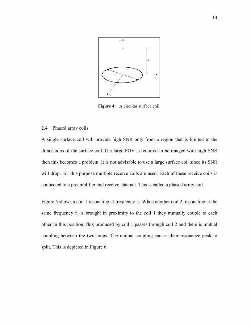
14
Figure 4: A circular surface coil.
2.4 Phased array coils
A single surface coil will provide high SNR only from a region that is limited to the
dimensions of the surface coil. If a large FOV is required to be imaged with high SNR
then this becomes a problem. It is not advisable to use a large surface coil since its SNR
will drop. For this purpose multiple receive coils are used. Each of these receive coils is
connected to a preamplifier and receive channel. This is called a phased array coil.
Figure 5 shows a coil 1 resonating at frequency f0. When another coil 2, resonating at the
same frequency f0 is brought in proximity to the coil 1 they mutually couple to each
other In this position, flux produced by coil 1 passes through coil 2 and there is mutual
coupling between the two loops. The mutual coupling causes their resonance peak to
split. This is depicted in Figure 6.

15
Figure 5: Single square coil resonating at frequency f0. Side dimension = x
This split in their resonant frequency causes a loss in sensitivity at frequency f0 for both
the coils. Hence during the building of a phased array coil, where a number of loops are
in close proximity to each other, it is important that mutual coupling between the loops
be kept as low as possible. This can be done by placing the two coils over each other
(overlapping the coils) at a position such that mutual inductance between them is zero. In
this position the net flux produced by coil 1 that passes through coil 2 is zero and the
loops are decoupled by geometric decoupling. This condition is shown in Figure 7.

16
Figure 6: Mutually coupled coils. (a) Splitting of resonant mode of coil 1 and coil 2 when they
are brought in proximity (b) B1 field of coil 1 passing through coil 2. The net flux through coil 2
not equal to zero Image (b) courtesy [28]
Figure 7: Mutually decoupled coils. (a) Dimensions of coils and overlap. Both coils resonate at
f0. (b) B1 field of coil 1 passing through coil 2, overlap position where net flux through coil 2
equals zero. Image (b) courtesy [28]
For two coils in the shape of a square loop of length x, overlapping two coils such that
the distance between their centers is approximately 0.9x would cause them to be nearly
perfectly isolated [1]. This distance could vary slightly depending upon factors such as
material of the loops, thickness of the loops, conductivity of the surrounding

17
environment in which the loops are placed. In fact, this work partially addresses this
issue by creating a ‘tunable’ geometrically decoupled coil.
The method mentioned above to eliminate mutual coupling between two coils can be
used when coils are placed adjacent to each other. Split in resonance peak of coils by
mutual coupling can also be caused by the next nearest neighboring coil, i.e. a coil
placed in proximity but which does not overlap with the coil. In Figure 8, coil 1 and coil
3 are next nearest neighbors. Also, coil 2 and coil 4 are next nearest neighbors.
Preamplifier decoupling is generally used to eliminate coupling between next nearest
neighboring elements.
Figure 8: Phased array coil of four elements. Each element is connected to an independent
preamplifier and receiver chain.
Phased array coils for this research are designed such that all the elements are decoupled
geometrically without the need of other forms of decoupling. A circularly polarized
trombone design birdcage is built to be used as a reference coil for comparison of
performance of the array coils.

18
3 MATERIALS AND METHODS
Five mouse-sized volume coils were constructed: a trombone design quadrature
birdcage coil, a two saddle quadrature coil, a four-channel array coil, a four channel
‘open’ array coil and a four channel ‘tunable’ decoupling array coil. All of these coils
operate at 200MHz. The coils were constructed on the outer surface of acrylic tubing
(Inner Diameter = 1.5 inches, Wall thickness = 0.125 inches). The sizes and types of
coils are given in Table 1.
Table 1: Five RF coils designed and fabricated for mouse MRI.
Coil
Type
Width
X-axis
(cm)
Height
Y-axis
(cm)
Length
Z-axis
(cm)
C1 Trombone Design Quadrature Birdcage 3.8 3.8 6.6
C2 Two saddle Quadrature coil 3.8 3.8 3.9
C3 Four Channel Array Coil 3.8 3.8 7.1
C4 Four Channel ‘Open’ Array Coil 3.8 3.8 6.0
C5 Four Channel ‘Tunable’ Decoupling Array Coil 3.8 3.8 8.0
Mouse coils C1 and C5 were built at the Magnetic Resonance Systems Laboratory
(MRSL) at Texas A & M University, College Station, Texas. Mouse coils C2, C3 and
C4 were built during a summer internship at G.E. Healthcare, Aurora,OH.
3.1 Circularly polarized trombone design birdcage coil (C1) A 16-leg high pass circularly polarized birdcage coil (ID = 3.8cms) was constructed
using the ‘trombone’ design [21,22]. A high pass design is chosen as it is more suitable
for high field strengths like 4.7T. The trombone design birdcage was fabricated using

19
copper tubes of two sizes. The smaller copper rods (K & S Engineering, Chicago, IL,
Ordered from Tower Hobbies, Part Number = LXBLV5) had an OD = 1/16”, Wall
thickness = 014”. The larger copper rods (K & S Engineering, Chicago, IL, Ordered
from Tower Hobbies, Part Number = LXBLV6) had an OD = 3/32”; Wall thickness =
.014”. The smaller copper rods slide into the larger ones such that the total rung length
and hence its inductance can be varied. The smaller copper rods were cut to 7cms length.
The larger copper rods were cut to 5 cms in length. Endrings were attached 2cms from
either ends of the rods. Hence the coil rung length can be varied from 5.5 cms, when the
smaller copper rods slide completely into the larger ones, to 9.5 cms. Both ports of the
coil resonate when the total length of the rungs is 6.6cms. Circular endrings were
machined using C30 PC board prototype from FR-4 sheets (thickness =0.16cms) (Figure
9(a)). The protel file for the endrings with 2 sizes of apertures is saved on the
d:/Sahil/endringsmall.pcb and d:/Users/Sahil/endringlarge.pcb (Figure 9(b)). Two of
these structures were stuck together using plastic epoxy. This was done to increase the
mechanical stability of the coil.
Figure 9: Circular endring of birdcage coil. (a) Photograph. (b) Screenshot of Protel file
endringsmall.pcb.

20
Figure 10 shows the birdcage coil C1 placed on a holder that centers the birdcage in the
X-Y plane in the 4.7T/40cm scanner. The holder was built in by a former student of the
lab.
Initial estimates of the required endring capacitor values was made using birdcage
builder [23]. On the settings tab of birdcage builder, the following values were entered:
Configuration = High pass; Number of legs = 16; Resonant Frequency = 200.03 MHz;
Type of endring = Rectangular; Type of leg = Tubular; Dimensions: Coil radius =
3.8cm; Leg Length = 7 cms; RF shield radius = 0cm (since no RF shield was used, 0
needs to be entered for this setting); ER Seg Width = 1cm. The birdcage builder gave an
initial estimate of 41.11pF as the endring capacitor values. No RF shield was used since
the coil size was small and it was anticipated that there would be negligible interactions
between the birdcage and the gradient and shim coils. The endring caps soldered were
47pF each (ATC 100 B series with tolerance +5%; American Technical Ceramics, New
York). Tunable (0-15pF) capacitors from Voltronics Corporation (Denville, NJ) were
used to tune one of the ports and match both ports of the birdcage coil.
Figure 10: Trombone design quadrature birdcage coil. (C1).

21
3.2 Two saddle quadrature coil (C2) Two saddles were constructed and wrapped around the acrylic cylinder. The loops of the
first saddle are placed at 0 and 180 degrees. The second saddle was identical to the first
saddle. It is wrapped around the acrylic cylinder such that its loops are placed at 90 and
270 degrees. Its position is adjusted such that the isolation between the two saddles is
optimized. Each saddle has 2 breakpoints. One breakpoint has a 15pF fixed and the other
breakpoint had a 0-15pF tunable capacitor. Figure 11(a) shows the CAD drawing of the
two saddle coil C2 while its photograph is shown in Figure 11(b).
Figure 11: Two saddle quadrature coil. (C2) (a) CAD drawing of coil. (b) Photograph of
coil.

22
3.3 Four channel array coil (C3)
Figure 12: Four channel array coil. (C3). (a) CAD drawing of coil (b) Photograph of
coil.
Figure 12(a) shows the CAD drawing of the four channel array coil C3 while its
photograph is shown in Figure 12(b). It consists of 4 rectangular loops which are
wrapped around an acrylic tube. The 1st loop wraps around half the circumference of the
acrylic tube (0°). A second identical loop wraps around the other half of the
circumference of the cylinder, 180 degrees opposite to the first (180°). The two loops
overlap from either side. This overlap is symmetrically adjusted to achieve maximum
isolation between the two loops. A 3rd loop is placed at a distance from the first two
loops along the length of the cylinder such that it overlaps slightly with the 1st and 2nd
loop. It is placed at 90 °, hence it symmetrically overlaps with both the loops. An
adjustable mechanism is provided such that its overlap with the 1st and 2nd loop can be

23
individually adjusted to achieve maximum isolation. The 4th loop is placed 180 degrees
opposite to the 3rd loop (270°). Isolation between the 4th and the 3rd loop is achieved in a
manner that is similar to the 1st and 2nd loops. The adjustable mechanism provided in the
3rd loop is also provided to achieve isolation with the 1st and 2nd loops. Hence it was
possible to geometrically decouple all four elements from one another by overlap.
3.4 Four channel ‘open’ array coil (C4) The four channel ‘open’ array coil consists of four loops. Two posterior loops wrap
around the half circumference of the acrylic tube (Loop 1 & 2). Overlap between these
loops was adjusted to give maximum isolation. Anterior loops (3&4) are similar in
shape to the posterior loops (1&2) but have extended regions to the right and left. The
extended regions on the left (of loop 1 & 2) wrap around the acrylic cylinder to overlap
with diagonal loops 3 and 4 respectively. Extensions on the right are provided, so as to
decrease coupling between diagonal loops. In the absence of these extensions, the
decoupling tabs would have to be much larger to compensate for coupling between
diagonal elements. This coil is designed to ‘open’ to provide easy access to the mouse.
Since the design lent itself to the modification, the acrylic tubing was cut in half and
hinged to facilitate the loading of animals. Figure 13 shows the CAD drawing of the coil
while its photograph is shown in Figure 14.

24
Figure 13: CAD drawing of four channel ‘open’ array coil. (C4).
Figure 14: Four channel ‘open’ array coil.
3.5 Four channel ‘tunable’ decoupling array coil (C5)
The four channel ‘tunable’ coupling coil C5 was fabricated by improving upon the
design of coil C3. Two areas were observed where the design of coil C3 could be
improved.

25
i) Firstly, the element geometry of coil C3 was such that in the area of overlap, a large
portion of one element was placed directly above the conductor of the other element.
This caused the element below to act as a shield to the one above, slightly reducing the
image quality. This is represented in Figure 15 where in the areas marked in red, the
conductor in blue (above) is shielded by a segment of the conductor in green (below).
Hence the element shape was modified such that at the overlap points the copper met at
right angles as shown in Figure 16.
Figure 15: Showing the region of overlap. The top coil (blue) is shielded by the bottom
coil (green).
Figure 16: Old element shape and modified new element shape.

ii) The overlap between the elements was
loading the coil with different loads, the decoupling
some loads dropped to well
the overlapping area (hence decoupling) could be adjusted for different loa
Coil C5, the ‘tunable’ decoupling coil
fabricated. While the overall footprint of the coil essentially remained ide
C3, the modified coil contained conductors at right angles and the
decoupling mechanisms. Figure 1
photograph is shown in Figure 1
Figure 17: Four channel
tween the elements was optimized and fixed for a particu
different loads, the decoupling between elements changed and for
to well below -20dB. Hence, mechanisms were designed
the overlapping area (hence decoupling) could be adjusted for different loa
Coil C5, the ‘tunable’ decoupling coil incorporated these modifications while being
he overall footprint of the coil essentially remained ide
the modified coil contained conductors at right angles and the
Figure 17(a) shows the CAD drawing of the coil
photograph is shown in Figure 17(b).
hannel “tunable” decoupling array coil. (C5) (a) CAD d
coil (b) Photograph of coil
26
for a particular load. On
changed and for
were designed by which
the overlapping area (hence decoupling) could be adjusted for different load conditions.
incorporated these modifications while being
he overall footprint of the coil essentially remained identical to coil
two ‘tunable’
(a) shows the CAD drawing of the coil C5 while its
(a) CAD drawing of

27
Each loop of the array coils C3, C4 and C5 has a single breakpoint with a 0-15pF
tunable capacitor. The coils were constructed using strips cuts from 0.125 inches wide
annealed copper (thickness= 0.25mm). G.E., HNS Rev 2 feedboards were used for
transmitting/receiving RF signals from the coils. The feedboards, originally designed to
operate at 1.5T were modified for imaging at 4.7 T. All unwanted components were
removed from the feedboards for IP protection. Inductor L2 and trimmer capacitor C3
form a balun at 200MHz. The average impedance provided by this LC circuit was 2.4kΩ
for the two saddle coil C2, 2.5kΩ for the four loops of C3 and 3.6kΩ for the four loops
of C4. Air core inductor L1, capacitor C4, and diodes D1 and D2 formed a passive
detuning circuit. During transmit, current introduced in the coil causes either D1 or D2 to
be forward biased. The LC circuit formed by L1 and C4 resonates at 200MHz, gives high
impedance between points a and b and detunes the loops. Capacitor C1 is the tuning
capacitor. Capacitor C2 is adjusted for matching the loop to 50 ohms. The equivalent
electrical circuit of a single coil element and feedboard are shown in Figure 18. A
cylindrical phantom with loading equivalent to a mouse was placed in the coil while
building and taking bench measurements of the coil. The cylinder (Diameter = 35mm;
Height = 75mm) was filled with 0.1M NaCl. Coil parameter measurements were
measured on RF network analyzer 8712ES (Agilent Technologies, Paulo Alto,CA).

28
Figure 18: Electrical circuit of a single coil element and feedboard. The coil element is tuned
by C1 and matched by C2. L1, C4, D1 and D2 form the passive detuning circuit. L2 and C3 form a
balun at 200MHz.
3.6 Supplementary apparatus
Mouse coils C2, C4 and C5 were receive only coils. For transmission, a detunable
birdcage coil built by a former student was used. The outer diameter of this coil was
15.5cms. Imaging was performed on the Varian Inova 4.7T/40cm system. The diameter
of the bore inside the gradients of the magnet was 26cms. This meant that the transmit
coil would not be centered when placed by itself in the magnet. It is important to place
the sample to be imaged in the homogeneous B0 field of the magnet. For the Varian
Inova 4.7T/40cm system, this region is the size of a 13 cm sphere. Hence it is required to
center the coil in the X, Y and Z directions. For this purpose, 2 acrylic half disks were
fabricated. Each had an inner diameter of 15.7 cms, equal to the outer diameter of the
birdcage coil, and a thickness of 0.5 inches. The first half disc has an outer diameter of
10 inches. This is attached to the end of the transmit birdcage coil that would be inserted

29
inside the gradients. The other half disc has an outer diameter of 12 inches and is
attached to the other end of the birdcage coil, which rests outside the gradient of the
magnet. These discs support the birdcage coil such that it is centered inside the magnet.
Both the disks are detachable by means of Velcro. Figure 19 shows the centering
mechanism attached to the birdcage coil.
Figure 19: Centering mechanism attached to the birdcage coil.
It is important to centre the receive coils inside the transmit coil since so that the sample
to be imaged lies in the homogenous region of the birdcage coil for uniform excitation of
its nuclei. The mechanism that centers the array coils is shown in Figure 20. This
mechanism can be used for centering the array coils C2, C4 and C5 inside the transmit
birdcage coil as the distance between the supporting structures is adjustable.

30
Figure 20: Mechanism centering the array coils inside the detunable birdcage coil.
To test the performance of the coils, a resolution structure that would fit inside the
cylindrical phantom was built (Figure 21). This was a 4cms x 1.5cms structure,
fabricated on a C30 PC board prototype from FR-4 sheets (thickness =0.16cms). It
consists of 7 rows of apertures. The first row has 3 apertures that have a diameter of
3mm. The number of apertures increases by 1, while the aperture diameter decreases in
each subsequent row. The last row had 10 apertures with diameter of 0.5mm. After every
row of apertures, an additional structure, which has the same number of holes of the
same diameter, is fixed perpendicular to the structure. This would show up in an axial
MR image in the XY plane whereas the original structure would show up in a coronal
image in the XZ plane. Thus the whole structure can be used to measure coil
performance in the XYZ planes.

31
Figure 21: Resolution structure. Dimensions = 4cms x 1.5cms, designed to fit inside the
cylindrical phantom.

32
4. RESULTS
S-parameter bench measurements were made on an RF network analyzer 8712ES
(Agilent Technologies, Paulo Alto, CA). Coil bench isolation measurements were made
using two different loads. Load 1 was a cylindrical phantom (Diameter = 35mm; Height
= 75mm) filled with 0.1M NaCl and 1g/l CuSO4. This represents the condition when the
coil is heavily loaded. Load 2 was a cylindrical phantom (Diameter = 25mm; Height =
97.5mm) filled with 1g/l CuSO4. This represents the condition when the coil is lightly
loaded.
Bench measurements for trombone design birdcage coil C1 indicate loaded coil isolation
between the two ports of -17.69dB. Both ports were matched to well under -20dB. The
data is shown in Table 2. Q measurements of the coil showed an unloaded Q of 105.86.
When the birdcage coil was loaded with Load 1, the Q of the coil measured was 20.80.
Hence the ratio of loaded to unloaded Q was 5.089.
Table 2: S Matrix [dB] for trombone design birdcage coil C1.
Port 1 Port 2
Port 1 S11 = -29.31dB S12 = -17.69dB
Port 2 S22 = -36.72dB
For the two saddle coil C2, the isolation between the two saddles was –21.06dB as
shown in Table 3. For these measurements, Load 1 with 0.1M NaCl and 1g/L CuSO4
was used. Saddle 1 was matched to -21.32 dB while saddle 2 was matched to -26.7 dB.

33
Table 3: S Matrix [dB] for two saddle coil C2.
Saddle 1 Saddle 2
Saddle 1 S11 = -21.32dB S12 = -21.60dB
Saddle 2 S22 = -26.7dB
S-parameter bench measurements, (Table 4), indicate average loaded (Load 1) coil
isolation between the elements of the four channel array coil C3 of - 19.63dB. All
elements were matched to well under -20dB. For the ‘open’ configuration, array coil C4,
the average isolation achieved was –18.06dB (data in Table 5).
Table 4: Matrix showing coupling [dB] for coil C3.
Table 5: Matrix showing coupling [dB] for coil C4.
The working of the detunable birdcage coil that was used for transmit with its PIN diode
driver used to detune the coil during receive was tested. The PIN diode driver had two
switches.
Element 1-Top 2-Bottom 3-Left 4-Right
1-Top - 27.6 -16.8 -25.2 -21.2
2-Bottom -29.7 -16.8 -18.3
3-Left -34.4 -19.5
4-Right -25.6
Element 1-Top 2-Top 3-Bottom 3-Bottom
1-Top -22.2 -19.6 -19.8 -16.8
2-Top -21.5 -16.0 -14.3
3-Bottom -37.0 -21.9
3-Bottom -16.2

34
Switch 1:
Position 1: Coil off for low input
Position 2: Coil off for high input
Switch 2:
Position 1: System control
Position 2: Manual override. Coil always “ON”
For the purpose of this test, images were acquired from this coil in T/R mode and in
transmit only mode for different positions of the two switches on the PIN diode driver. A
cylindrical phantom (O.D = 6.7cm, Height = 9.7cm) filled with 1g/L CuSO4 was used.
Images were acquired with under following cases:
Case I: Birdcage in T/R mode. PIN diode driver not connected. Images were acquired
from the detunable birdcage coil and are shown in Figure 22.
Figure 22: T/R images of CuSO4 phantom. (a) Axial Image (b) Coronal Image.
Case II: Switch 1: Coil off for low input. Switch 2: System Control. Images acquired
from the birdcage for this case are shown in Figure 23.

35
Figure 23: Images of CuSO4 phantom. (a) Axial Image (b) Coronal Image.
Case III: Switch 1: Coil off for low input. Switch 2: Manual override. Coil always “ON”.
Images acquired from the birdcage for this case are shown in Figure 24.
Figure 24: Coronal image of CuSO4 phantom.
Case IV: Switch 1: Coil off for high input. Switch 2: Manual override. Coil always
“ON”. Images acquired from the birdcage for this case are shown in Figure 25.

36
Figure 25: Coronal image of CuSO4 phantom.
Looking at the images from different positions of the switches, it was concluded that
when Switch 2 is in Position 2: Manual override. Coil always “ON”, the coil’s detuning
circuit is deactivated. The coil operates in T/R mode in this position. For operating the
coil in Transmit only mode, Switch 2 needs to be in Position 1: System Control. The
images from Case I (Coil in T/R mode) and Case II (Coil in transmit only mode) were
analyzed for SNR calculations using an in house code. Figure 26 & 27 show images
from the analysis of the phantom. In the code, images have an intensity range of [1 256].
All pixels above 80 (red pixels) are considered image pixels while below 80 (blue
pixels) are considered noise pixels. For axial images of the phantom the SNR in T/R
mode was 206.4384 while in transmit only mode it was 35.0303. For coronal images of
the phantom the SNR in T/R mode was 114.4919 while in transmit only mode it was
11.1378. Thus, there is an 83.03% and 90.02% reduction in SNR in the two cases
respectively which shows good detunability of the birdcage coil.

37
Figure 26: Processed axial images of CuSO4 phantom. (a) T/R mode; SNR=206.4384 (b)
Transmit only mode; SNR=35.0303.
Figure 27: Processed transverse images of CuSO4 phantom. (a) T/R mode; SNR=114.4919 (b)
Transmit only mode; SNR=11.1378.
For adjusting the amount of decoupling between the top and bottom elements, a flux
blocking paddle, was used to control the surface area of the overlap, and thus the amount
of mutual inductance. The rectangular flux blocking paddles (50mm X 13mm) were
machined using C30 PC board prototype from FR-4 sheets (thickness = 0.16cms). To
verify the ability to control the decoupling by changing the area of overlap covered by
the paddle, the elements were matched and tuned to 50 ohms and the decoupling
measurements were collected at different positions of the paddle at intervals of 2mm.
Figure 28 shows the decoupling paddle at different overlapping positions. Figures 30 –

38
31 show the graphs for variations in decoupling values between elements for different
positions of the decoupling paddles. With the NaCl load, S21 showed a minimum value
of – 23.9 dB at 1.6 cm while with the CuSO4 load the minimum value was – 27.9 dB at
3.2 cm, a difference of about 1.6cms in the position of the paddle. With the NaCl load,
S34 showed a minimum value of – 21.0 dB at 2.2 cm while with the CuSO4 load the
minimum value was – 28.6 dB at 3.0 cm, a difference of about 0.8cms in the paddle
position.
Figure 28: Decoupling paddle at different overlap positions. (a) 1cm overlap (b) 2cm overlap
(c) 3cm overlap (d) 4cm overlap.
Table 6: S21 values at different positions of the paddle for two loads Paddle position
[cm]
S21 with Load 1 [dB]
S21 with Load 2 [dB]
Paddle position [cm]
S21 with Load 1 [dB]
S21 with Load 2 [dB]
0 -18.5 -9.3 1.6 -23.9 -11.1
0.2 -18.6 -9.4 1.8 -23.2 -11.7
0.4 -18.6 -9.4 2 -22.3 -12.4
0.6 -18.9 -9.5 2.2 -21.2 -13.1
0.8 -19.4 -9.7 2.4 -19.8 -14.2
1 -20.4 -9.7 2.6 -18.6 -15.5
1.2 -21.9 -9.9 2.8 -17.5 -17.5
1.4 -23.4 -10.5 3 -16 -20.5

39
Paddle position (cm)
S21 [dB]
Figure 29: Graph of S21 vs. paddle position.
Table 7: S34 values at different positions of the paddle for two loads. Paddle position
[cm]
S34 with Load 1 [dB]
S34 with Load 2 [dB]
Paddle position [cm]
S34 with Load 1 [dB]
S34 with Load 2 [dB]
0 -15.9 -9.1 2.2 -21 -17.1
0.2 -16.1 -9.1 2.4 -20.7 -18.6
0.4 -16.1 -9.1 2.6 -20 -21.1
0.6 -16.1 -9.1 2.8 -19.5 -25.2
0.8 -16.5 -9.4 3 -18.9 -28.6
1 -17.1 -10.1 3.2 -18 -26.5
1.2 -18.2 -10.9 3.4 -17.1 -22.4
1.4 -19.1 -11.6 3.6 -15.9 -18.9
1.6 -20.2 -12.5 3.8 -15.5 -17
1.8 -21 -13.9 4 -14.4 -15.3
2 -21.3 -14.9
-30
-25
-20
-15
-10
-5
0
0 1 2 3 4
NaCl
CuSO4

40
Paddle position (cm)
S34 [dB]
Figure 30: Graph of S34 vs. paddle position.
For adjusting the amount of decoupling between the diagonal elements surface area of
the overlap was controlled by changing the length of elements 3 and 4. The mechanism
developed was such that the overlap area with the other individual elements could be
adjusted. Two sizes of copper rods were used. 4mm length of the larger copper rods (OD
= 3/32”; Wall thickness = .014”) were cut. These were fixed to the acrylic cylinder.
Smaller copper rods of OD = 1/16”, Wall thickness = 014” were attached to the element
copper and slide into the larger copper rods. With this mechanism, the overlap area
between any 2 diagonal elements can be individually adjusted. Figure 31 shows this
mechanism. To verify the ability to control the decoupling by changing the area of
overlap, diagonal elements were matched and tuned to 50 ohms and the decoupling
measurements were collected at different positions of overlap at intervals of 0.5mm.
-35
-30
-25
-20
-15
-10
-5
0
0 2 4 6
NaCl
CuSO4

41
Figure 31: Showing different positions of overlap. (a) 0 mm overlap (b) 5mm overlap.
Figures 32-34 show graphs of variations in decoupling values at different positions of
overlapping between elements for two different loading conditions. Tables 8 – 11 show
the corresponding numerical values.
Table 8: S32 values at different overlap positions for two loads.
Position (mm)
S34 with Load 2 [dB]
S34 with Load 2 [dB]
0 -14 -9.3
0.05 -15.9 -9.9
0.1 -17.5 -11.2
0.15 -18.6 -12.8
0.2 -21.3 -14.2
0.25 -22.7 -16.1
0.3 -24.8 -19.4
0.35 -31.3 -20.5
0.4 -41.2 -25
0.45 -36.2 -29.2
0.5 -30 -26.5

42
Overlap length (mm)
S32[dB]
Figure 32: Graph of S32 vs. overlap length.
Table 9: S31 values at different overlap positions for two loads.
Position (mm)
S31 with Load 1 [dB]
S31 with Load 2 [dB]
0 -25.3 -36
0.05 -29.9 -33
0.1 -34.9 -26
0.15 -31.2 -21.3
0.2 -24.1 -18.4
0.25 -21.7 -16.2
0.3 -18.5 -14
0.35 -17.3 -13.6
0.4 -15.3 -12.2
0.45 -14.7 -11.6
0.5 -13.9 -11.3
-50
-40
-30
-20
-10
0
0 0.2 0.4 0.6
NaCl
CuSO4

43
Overlap length (mm) S31[dB]
Figure 33: Graph of S31 vs. overlap length.
Table 10: S41 values at different overlap positions for two loads.
Position (mm)
S41 with Load 1 [dB]
S41 with Load 2 [dB]
0 -23.2 -16.8
0.05 -19.2 -11.8
0.1 -17.3 -9.8
0.15 -15.9 -8.7
0.2 -14.4 -8.4
0.25 -13.2
0.3 -12.4
0.35 -11.8
0.4 -11.3
0.45 -11.1
0.5 -10.6
-40
-35
-30
-25
-20
-15
-10
-5
0
0 0.2 0.4 0.6
NaCl
CuSO4

44
Overlap length (mm)
S41[dB]
Figure 34: Graph of S41 vs. overlap length.
Table 11: S42 values at different overlap positions for two loads.
Position (mm)
S42 with Load 1 [dB]
S42 with Load 2 [dB]
0 -16.7 -17.2
0.05 -20 -23.5
0.1 -22.3 -28.4
0.15 -25.5 -22.1
0.2 -29.5 -17.6
0.25 -40.1 -15
0.3 -34.5 -13.5
0.35 -26.8 -12.2
0.4 -22.1 -11.4
0.45 -20.5 -10.9
0.5 -18.8 -10.4
-25
-20
-15
-10
-5
0
0 0.5 1
NaCl
CuSO4

45
Overlap length (mm) S42[dB]
Figure 35: Graph of S42 vs. overlap length.
-45
-40
-35
-30
-25
-20
-15
-10
-5
0
0 0.2 0.4 0.6
NaCl
CuSO4
46
5. DISCUSSION
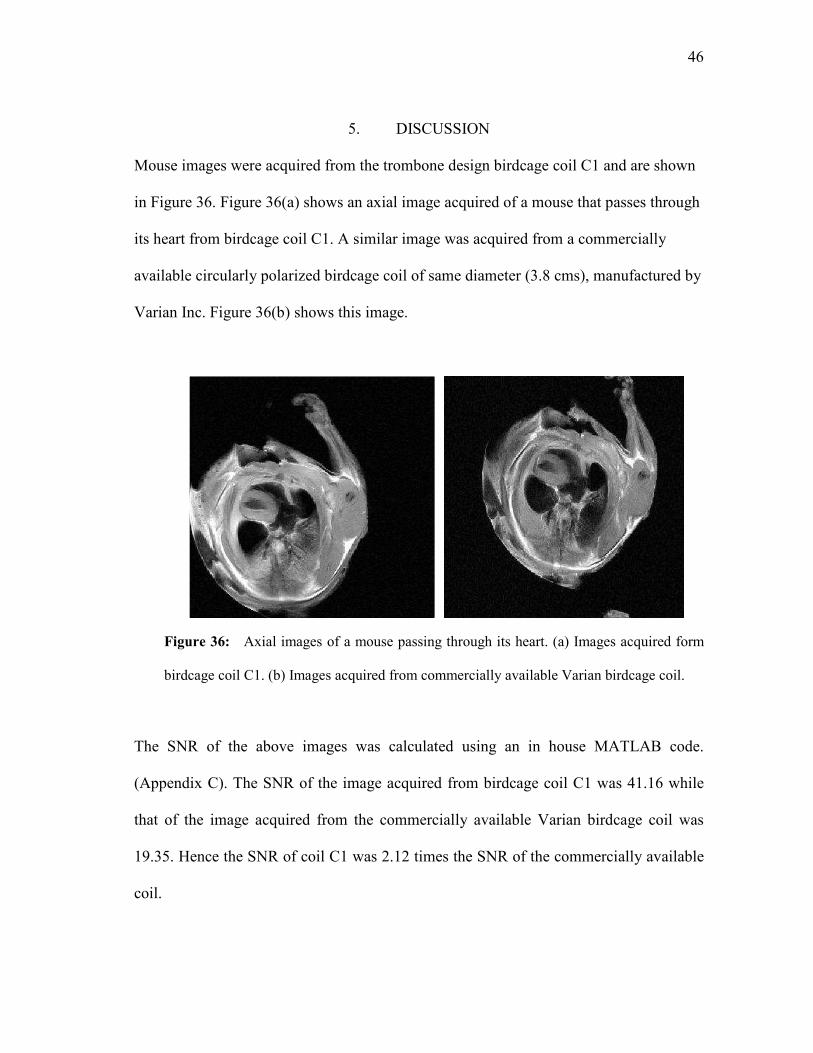
Mouse images were acquired from the trombone design birdcage coil C1 and are shown
in Figure 36. Figure 36(a) shows an axial image acquired of a mouse that passes through
its heart from birdcage coil C1. A similar image was acquired from a commercially
available circularly polarized birdcage coil of same diameter (3.8 cms), manufactured by
Varian Inc. Figure 36(b) shows this image.
Figure 36: Axial images of a mouse passing through its heart. (a) Images acquired form
birdcage coil C1. (b) Images acquired from commercially available Varian birdcage coil.
The SNR of the above images was calculated using an in house MATLAB code.
(Appendix C). The SNR of the image acquired from birdcage coil C1 was 41.16 while
that of the image acquired from the commercially available Varian birdcage coil was
19.35. Hence the SNR of coil C1 was 2.12 times the SNR of the commercially available
coil.

47
T/R images from four channel array coil C3 were acquired on a 4.7T/33cm scanner
supported by a Varian Unity Inova console. The imaging parameters were: Spin Echo
Images; TR/TE=300/30msec; Matrix Size =128x128; Field Of View = 100mm; Slice
Thickness = 3mm; Number of averages = 2. One set of images from each individual
elements were acquired when the other elements were terminated to 50Ω. These images
are shown in Figure 37. Another set of images was acquired with the other elements
open circuited (Figure 38). Images obtained under these two conditions showed very
slight differences, confirming the elements were well isolated and offering promise for
future work based on geometric decoupling techniques alone. These images were
included in the accepted ISMRM abstract “Geometrically Decoupled Phased Array Coils
for Mouse Imaging” and are shown below.
Figure 37: Images with other loops terminated to 50Ω. (a) Sagittal image; top element (b)
Sagittal image; bottom element (c) Coronal image; left element (d) Coronal image; right
element.

48
Figure 38: Images with other loops open circuited. (a)Sagittal image; top element (b)Sagittal
image; bottom element (c)Coronal image; left element (d)Coronal image; right element.
Receive only images were acquired from the four channel ‘open’ array coil C4 were on
the 4.7T/40cm scanner. An existing detunable birdcage was used as the transmit coil.
Sagittal images were obtained to observe the sensitive regions from the two top and the
two bottom elements; plane is shown in Figure 39(e). The images from all four elements
are shown in Figure 39(a-d). Images were acquired from all four elements when the coil
was closed (Figure 39(a) and 39(b)). Another set of images was acquired from the
bottom two elements when the coil was opened (Figure 40(c) and 40(d)).
(e)
Figure 39: Images with coil closed. (a) Top element 1 (b) Top element 2 (c) Bottom element 1
(d) Bottom element 2 (e) Coronal imaging plane.

49
Figure 40: Images with coil open. (a) Bottom element 1 (b) Bottom element 2.
Receive only coronal images were acquired from mouse coil C5 to observe the sensitive
regions of the left and the right elements. Images are shown in Figure 41(a-b). The
coronal imaging plane is shown in Figure 41(c). Imaging parameters were: TR/TE =
300/30; Matrix Size = 128x128; FOV = 100mm; Slice Thickness = 3mm; Nav = 2. On
observing the images closely, we saw that the each of the sensitive regions of the two
elements covered almost the entire phantom. Hence, to verify if this coil could be used
for parallel imaging, the images were analyzed for the coil g-factors.
(c)
Figure 41: Coronal Images. (a) Left Element (b) Right element (c) Coronal imaging plane.

50
The analysis of the images was done by Dr. Jim Ji, a professor at the Department of
Electrical and Computer Engineering. Following were results of his analysis:
Case I - Full FOV: In the original acquisition, the FOV is set to be roughly 4 times of the
size of the phantom along the horizontal. Figure 42 shows the magnitude and phase
images of the coils in this full FOV. Phase images show that the phase along the
horizontal direction is quite constant. This does not help the coil g-factor. As seen in
Figure 43, the g-factor is not bad in this case of the full FOV. But it doesn’t make
practical sense to apply parallel imaging in the full FOV, because we can simply reduced
the FOV to half without create any real aliasing.
Figure 42: Magnitude and phase plots of full FOV images. (a) Coil 1 magnitude image (b) Coil
1 phase image (c) Coil 2 magnitude image (d) Coil 2 phase image.
1
2
3
4
5
6
7
-3
-2
-1
0
1
2
3
(C)
1
2
3
4
5
(D)
-3
-2
-1
0
1
2
3
(A) (B)

51
Figure 43: Full FOV g factor map.
Case II – Reduced FOV – Figure 44 shows the coil magnitude and phase images with
the FOV truncated to the phantom region, which is the actual FOV of 256x64 pixels
which covers the phantom area only. Now, the g-factors become worse as shown in
Figure 45. In this case, the parallel imaging performance (reduction along horizontal)
will not be optimal, as the noise will be amplified by 100 times in lots of pixels.
50 100 150 200 250
50
100
150
200
250
20
40
60
80
100
120

52
Figure 44: Magnitude and phase plots of reduced FOV images. (a) Coil 1 magnitude image (b)
Coil 1 phase image (c) Coil 2 magnitude image (d) Coil 2 phase image.
Figure 45: Reduced FOV g factor maps. (a) Scale 0 - 600 (b) Scale truncated to 100.
20 40 60
50
100
150
200
250
100
200
300
400
500
600
(B)
20 40 60
50
100
150
200
250
10
20
30
40
50
60
70
80
90
1
2
3
4
5
6
7
-3
-2
-1
0
1
2
3
(C)
1
2
3
4
5
(D)
-3
-2
-1
0
1
2
3
(B)(A)
(A)

53
Obviously it does not make sense then to accelerate in the “left-right” direction using
these coils. Accelerating in the top-bottom direction might be possible, although the
optimal imaging plane is not obvious as the coils are rotated 90 degrees from one
another (one’s pattern is better used in coronal imaging and one’s pattern is better used
in sagittal imaging). In addition, the phase encoding direction (direction of acceleration)
in an image is typically not set to be the longest dimension so this would be a very non-
standard configuration for several reasons.
Before the apparatus was inserted into the magnet for imaging, conditions during
transmit and receive were simulated on the bench to test the active detuning circuit of the
birdcage and the passive detuning circuit of the array coils. During the transmit phase of
imaging, the birdcage coil needs to be tuned to 200MHz. It then generates a
homogeneous B1 field inside its volume. The array coils need to be detuned from
200MHz so that they do not resonate and couple to the transmitting birdcage coil,
distorting its homogeneous B1 field. Inside the magnet, the B1 field generated by the
birdcage coil would induce current in the coil which would turn on the diodes D1 and D2
(refer Figure 18) thus detuning the array coils. To simulate this condition on the bench,
the diodes D1 and D2 on the feedboards were shorted. The simulating conditions showed
that the arrays detuned perfectly during transmission and the S21 between each element
of the array coil and the birdcage was > - 25dB. During the receive phase of imaging, the
array coils are tuned to 200MHz and acquire RF signal generated by the sample. The
birdcage coil that is used to transmit needs to be detuned from 200MHz so it does not

54
induced current in the array coils thereby distorting the reception of the RF signal
generated by the sample. To simulate these conditions on the bench, the PIN diode
driver circuit was switched on. It provided DC current to all the PIN diodes on the
birdcage, thereby detuning it. The isolation between the elements of the array coil and
the birdcage was > -25dB, showing good detunability of the birdcage coil.
Figure 46: Showing S21 [dB] measurements with flux probe.
After examining the axial images from coil, two half moon structures were seen. It was
assumed that this was coil coupling between elements. Hence bench measurements were
made for getting accurate measurements of coil coupling. Two elements of the coil were
connected to the port 1 and port 2 of the network analyzer respectively. S21 measurement
on the network analyzer showed an isolation of -16.01dB. Then, coil 2 was disconnected
and terminated to 50Ω. A flux probe was connected to port 3 of the network analyzer.
The flux probe was used to make current measurements on the copper of the elements

55
themselves. S32 and S31 measurements were made on various points on the elements
themselves. Figure 46 shows the measurements at different positions on the coil copper.
The differences in the measurements were approximately -15dB. This matched the S21
measurements when the two elements were connected to the network analyzer. Hence it
was concluded that the measurement seen on the network analyzer was indeed an
accurate indication of the decoupling between the elements.

56
6. CONCLUSION
A well performing circularly polarized birdcage coil for mouse imaging was fabricated.
The dimensions of this coil were Diameter = 3.8cms, Length = 6cms. Hence it can
efficiently image a 68 cm³ cylindrical volume. Phantom or mouse images can be
acquired with this birdcage. Mouse images were acquired from this birdcage showed an
SNR of ≈ 40; while the SNR of similar images acquired from a commercially available
circularly polarized Varian birdcage coil was ≈19. Hence the fabricated birdcage had
almost twice the SNR of the Varian birdcage coil over a larger FOV (in the Z direction).
High resolution mouse images can be taken from this birdcage coil. Mouse imaging is of
increasing interest within the Biomedical Engineering Department and also at the Vet
school at Texas A & M University. Hence this coil can be useful in collaborations within
the department and the university.
Bench and imaging results from four channel array coil C3 (the geometrically decoupled
array coil built as a prototype during the summer internship) and bench results from the
four channel ‘open’ array coil, C4, showed that the coils were indeed decoupled
geometrically, offering promise for future work based on geometric decoupling
techniques alone. These results were included in the accepted ISMRM abstract: S. P.
Bhatia, Y. Guan, F. J. Robb, M. P. McDougall. “Geometrically decoupled phased array
coil for mouse imaging.” Proceedings of the International Society of Magnetic
Resonance in Medicine (2009).

57
Two mechanisms for ‘tunable’ decoupling between overlapping elements of an array
coil were presented: tunable paddle decoupling and variable overlap decoupling. Both
these mechanisms showed good “tunability” of decoupling. Both mechanisms were able
to optimize decoupling of the elements over a wide range of loading conditions. Wide
ranges of loading conditions are encountered during the usage of a coil. Loading
conditions change with change in the phantom to be imaged. They changed when the
coil is switched between phantom imaging and mouse or other animal imaging. They
change when bench measurements of the coil need to be performed, such as measuring
unloaded Q of the coil. Imaging different animals with the coil also provide different
loading conditions. Under different loading conditions, different overlap is required for
isolating overlapping elements. These mechanisms help optimizing decoupling between
overlapping coils for different loading conditions. This also prevents adjusting the
overlap by resoldering the overlapping conductors of the elements, which can be tedious
and iterative.

58
REFERENCES
1. Roemer PB, Edelstein WA, Hayes CE, Souza SP, Mueller OM. 1990. The NMR
phased array. Magnetic Resonance in Medicine 16:192–225.
2. Hayes CE, Hattes N, Roemer PB. 1990. Volume imaging with MR phased arrays.
Magnetic Resonance in Medicine. 18:309-319.
3. Edelstein WA, Schenck JF, Mueller OM, Hayes CE. 1987. Radio frequency field
coil for NMR. U.S. patent 4 680 548.
4. B. Keil, Wald LL, Wiggins GC , Triantafyllou C, Meise FM, Klose KJ, Heverhagen
JT. 2008. 20-Channel mouse phased-array coil for clinical 3 tesla MRI scanner. In:
Proceedings of the International Society of Magnetic Resonance in Medicine.
16:1105 p.
5. Beck BL, Blackband SJ. 2001. Phased array imaging on a 4.7T/33cm animal
research system. Review of Scientific Instruments. 72:11:4292-4294
6. Ullmann P, J. S., Hennel F, Nauerth A, Panagiotelis I, Ruhm W, Hennig J. 2004.
High field parallel imaging in small rodents. In: Proceedings of the 11th ISMRM,
Kyoto. 11:1610 p.
7. Wosik J, Nesteruk K, Xie LM, Kamel M, Xue L, Bankson JA. 2004.
Superconducting 200 MHz "phased" array for parallel imaging. In: Proceedings of
the International Society of Magnetic Resonance in Medicine 4.
8. Gareis D, Wichmann T, Lanz T, Melkus G, Horn M, Jakob PM. 2007. Mouse MRI
using phased-array coils. NMR in Biomedicine. 20:326-334

59
9. Beck BL, Plant DH, Grant SC, Thelwall PE, Silver X, Mareci TH, Benveniste H,
Smith M, Collins C, Crozier S, Blackband SJ. 2002. Progress in high field MRI at
the University of Florida. Magnetic Resonance Materials in Physics, Biology and
Medicine. 13:152-157
10. Oduneye SO, Menon RS. 2008. A 4-channel transceive surface coil array for small
animal imaging at 9.4T. In: Proceedings of the International Society of Magnetic
Resonance in Medicine. 16:1100 p.
11. Wang Z, Tabbert M , Junge S, Gordon RE, Yang QX, Smith MB, Collins CM.
2008. Optimization of phased array coils for small-animal MRI at 9.4T. In:
Proceedings of the International Society of Magnetic Resonance in Medicine.
16:1103 p.
12. Nascimento GC, Paiva FF, Silva AC. 2008. An inductively decoupled coil array for
parallel imaging of small animals at 7T. In: Proceedings of the International Society
of Magnetic Resonance in Medicine. 16:1099 p.
13. Zhang X, Webb AG. 2004. Design of a coil array for mouse imaging at 14.1 T. In:
Proceedings of the International Society of Magnetic Resonance in Medicine. 11:39
p.
14. Bock NA, Konyer NB, Henkelman RM. 2003. Multiple-mouse MRI. Magnetic
Resonance in Medicine. 49:158-167.
15. Zhang X, Webb A. 2005. Design of a four-coil surface array for in vivo magnetic
resonance microscopy at 600 MHz. Concepts in Magnetic Resonance Part B
(Magnetic Resonance Engineering). 24B(1):9.

60
16. Fan X, Mickiewicz EJ, Zamora M, Karczmar GS, Roman BB. 2006. Comparison
and evaluation of mouse cardiac MRI acquired with open birdcage, single loop
surface and volume birdcage coils. Physics in Medicine and Biology. 51 9.
17. Doty FD, Entzminger G, Kulkarni J, Pamarthy K, Staab JP. 2007. RF coil
technology for small-animal MRI. NMR in Biomedicine. 20:304-325
18. Wargo CJ, Gore JC, Avison MJ. 2008. Four Channel Array for 9.4T Animal Studies.
In: Proceedings of the International Society of Magnetic Resonance in Medicine.
16:1102 p.
19. Ramirez MS, Bankson JA. 2008. Multiple-mouse MRI with multiple arrays of
receive coils (MARCs). In: Proceedings of the International Society of Magnetic
Resonance in Medicine. 16 :1106 p.
20. Fischer S, Meise FM, Kronfeld A, Alessandri B, Schreiber WG. 2008. Modular 4-
element coil array constructed of simple coil loops without extra shielding for the
simultaneous MRI of multiple small animals. In: Proceedings of the International
Society of Magnetic Resonance in Medicine. 16:1101 p.
21. McDougall MP, Brown DG, Spence D, Wright SM. 2001. A Low-pass trombone
birdcage coil with broad tuning range. In: Proceedings of the International Society of
Magnetic Resonance in Medicine. 9: 1092 p.
22. Xu Y, Tang P. 1997. Easy fabrication of a tunable high-pass birdcage resonator.
Magnetic Resonance in Medicine. 38: 168-172

61
23. Chin CL, Collins CM, Li S, Dardzinski BJ, Smith MB. 1998. Birdcagebuilder. 1.0:
Copyright Center for NMR Research, Department of Radiology, Penn State University
College of Medicine.
24. Pruessmann P, Weiger M, Scheidegger MB, Boesiger P. 1999. SENSE: Sensitivity
encoding for fast MRI. Magnetic Resonance Medicine. 42:952–962
25. Wiesinger F, Boesiger P, Pruessmann KP. 2004. Electrodynamics and ultimate SNR
in parallel MR imaging. Magnetic Resonance in Medicine. 52(2):376-90
26. Jin J. 1999. Electromagnetic Analysis and Design in Magnetic Resonance
Imaging. CRC Press, Boca Raton, FL. 146 – 149
27. Wright, S. M. 2007. Principles of Magnetic Resonance Imaging. 37.
28. Ke, F. 2005. SNR as a function of preamp impedance, coil to coil
distance, coil to phantom distance (loading), frequency.
29. Kelton JR, Magin RL, Wright SM. 1989. An algorithm for rapid image acquisition
using multiple receiver coils. In: Proceedings of the 8th Annual Meeting SMRM,
Amsterdam. 1172 p

62
APPENDIX
(A) Design considerations for array coils
In an MRI experiment, we can localize the signal that is acquired by the RF coil. But
noise is collected from the entire region of sensitivity of the coil. Tailoring the coils such
that their sensitive region covers only the volume to be imaged so that the noise is
gathered from the smallest possible volume increases the SNR of an MR image. Initially,
this was the motivation for the development of phased array coils: increased SNR over a
large FOV. To obtain the maximum SNR from an array coil, however, the signals from
each coil need to be combined in an appropriate manner. If separate coils images are
simply added, i.e. equal weights are given to coils near and far away from a particular
pixel of interest, then coils that are far away from the pixel of interest will not have
significant sensitivity near that pixel and hence will add only noise to that pixel. The
technique to combine signals for maximum SNR was presented by Roemer et al [1].
They also suggested different techniques of combining signals from an array coil. It was
observed that to combine the signals from an array coil for maximum SNR, detailed
knowledge of the spatial sensitivities of each of the coils was to be known. But in
general we do not know the spatial sensitivity of the coils. Hence another technique was
suggested, the sum of squares technique. In this technique, each pixel value is the square
root of the sum of the squares of the pixel values corresponding to individual coils in the
array. For this method, no knowledge of the spatial sensitivity of each coil in the array is
required. For most images, the sum of squares combination method provides an SNR of
within ten percent of the maximum SNR image.

63
Acceleration in MRI images.
Only one position in k space can be sampled at one time, hence to decrease scan time it
was important to travel faster through k space. Increasing gradient performance was one
way of reducing minimum scan time. In 1999, it was observed by Kelton et al [29], that
the receiver coils sensitivity has a spatial encoding effect that is complimentary to
gradient encoding. Thus, if multiple receiver coils were used in parallel, like a phased
array coil, the time required to scan the Fourier k space can be reduced, providing
acceleration in acquiring MRI images. The technique suggested reducing the number
Fourier encoded steps, i.e. k space readouts and was called Sensitivity Encoding
(SENSE).; .
SR in acceleration
Excessive noise in the reconstructed image is considered as the main limit to parallel
imaging [25]. The equation for SNR for parallel imaging as given by Pruessmann et al
[24]
SNRR = SNR0 / g √R [A.1]
SNR0 = Baseline SNR which depends on the performance of the system, detector
efficiency, pulse sequence design and various other factors.
R = Reduction factor i.e. factor by which k space samples is reduced
g = geometry factor

64
Reduction factor R
Each point in the k space contains both signal and noise. From the property of the
Fourier transform, each point in the image domain is formed by the weighted sum of all
points in the Fourier domain (k space). Thus, just as increasing the number of averages
increases the SNR by a factor of square root of the number of averages, reducing the
number of readouts in k space decreases the SNR by a factor of the square root of the
reduction factor, R.
g factor of array coils
As seen from Eqn. A.1, the SNR for parallel imaging is inversely proportional to a term
called the g factor. Hence the SNR degrades as the g factor value increases. G factor
values are always greater than or equal to 1. Hence g factor values should be as close to
1 as possible. What the g factor is and what degrades the g factor will be discussed
below.
Receiver coil sensitivity has a spatial encoding effect that adds to the encoding effect of
the gradients. This encoding ability arises from the fact that each coil has different
sensitivities for each pixel in the FOV. The sensitivity is a complex function, so both
spatially varying magnitude and/or phase help encoding ability. The g factor or the
geometry factor describes this encoding ability of the array coils. It describes the ability
of the array coil configuration to separate pixels superimposed by aliasing in the reduced
FOV. G factor noise arises when the coil sensitivities are too similar. When the

65
sensitivities of the coils are too similar, the sensitivity matrix S as defined by
Pruessmann et al [24] becomes ill conditioned. This happens if the coils lack spatial
relative variations in patterns and can occur when are too close to each other, or if the
FOV considered is very small. When an ill conditioned matrix is inverted and multiplied
to another vector then solutions are produced that are extremely sensitive to small
changes in the vector i.e. noise in the vector are heavily amplified. The unfolding matrix
for SENSE reconstruction U [24] includes the inversion of the sensitivity matrix S. In
this case, when an ill conditioned S is inverted and multiplied to, a [24], the aliased data
matrix, the noise in vector a is heavily amplified. Hence it is important that the
sensitivity matrix is not ill conditioned. Or in simpler terms, the g factor values are kept
as close to 1 as possible. It should be noted that the g factor noise originates from the
matrix a, the aliased input data, not in the sensitivity matrix S. However the sensitivity
matrix amplifies this noise.
G factor varies from pixel to pixel across the image domain, as the coil sensitivities vary
in this way; hence g factor maps are required for description of the performance of the
array coil with respect to g factors. It is critical that the array is designed such that g
factor achieved is as close to 1 as possible. G factors of ≈ 1.2 are tolerable depending
upon the application.
Decoupling arrays.
It is important that one must decouple the elements of an array. When two coils
resonating at frequency f0 are in proximity of each other they mutually (inductively)

66
couple to each other. The mutually coupling causes their resonances to split. This split in
their resonant frequency causes a loss in sensitivity at frequency f0 for both the coils.
Hence during the building of a phased array coil, it is important that mutual coupling
between the loops be kept low. The splitting of resonances can be prevented when the
coils are decoupled to about – 10dB. Further beyond, it is important that we decouple the
coils to about – 15dB so that each individual element can be independently be tuned and
matched to Z = R + j X = 50 + j 0 ohms. If the coils are not independently tuned and
matched to 50Ω, then there would be SNR loss due to signal return loss. By preventing
resonance split and being able to tune/match to 50Ω, we are trying to improve the
baseline SNR, SNR0. Ideally – 20 dB decoupling between elements is considered as a
good decoupling value. If we try to further reduce coupling no significant improvement
in baseline SNR occurs but reduces signal and noise correlation between the elements.
Conclusion for design of array coils
In order for one to design array coils, both decoupling the elements of an array and
considering the g factors are important. The ideal condition would be when g factors of
around 1 are achieved and the decoupling values of – 20 dB are achieved. However if a
situation arises where coupling needs to be compromised for better g factor values, one
can compromise on decoupling such that coils do not have resonance split and can be
tuned and matched separately, so that the baseline SNR0 does not significantly
deteriorate. This value should be ≈ – 15 dB. Increase in G factors up to 1.2 can be
tolerated. If geometric decoupling is used, then adjacent coils need to be overlapped.

67
Overlapped coils have high g factors close to the coils, while underlapped coils have
lower g factors close to the coils. Underlapped coils are no longer geometrically
decoupled, so other methods have to be employed to minimize coupling that reduces
baseline SNR.
(B) How to build a birdcage coil.
STEP 1: Know the dimensions of volume to be imaged.
For mouse coils, 3.8 cm diameter coils is the standard used in literature. Length of mice
is around 4 cms, hence the length of birdcage chosen was so that it resonates at a length
between 5 to 7 cms. Since the homogenous region of the birdcage in the z direction is
slightly smaller than its rung length, choose the total rung length such that it is slightly
longer than the length of volume to be imaged.
STEP 2: Determine the resonant frequency from field strength of the magnet.
For a 4.7T magnet, the resonant frequency for 1H imaging is 200MHz.
STEP 3: Decide on the design of the birdcage
Choose from having a low pass/ high pass or band pass design of birdcages. At high
field strengths of 4.T, high pass design is preferred over the low pass design since
capacitor values for resonance in low pass birdcage coils tend to be very low (<5pF) at
high field strengths. The tolerance at these low values of capacitors cause large changes
in the actual values. Choose between a linearly polarized or circularly polarized design.

68
The circularly polarized design provides a √2 improvement in SNR and should be
preferred.
STEP 4: Choose the number of rungs in the birdcage
Higher the number of rungs, the larger the homogenous region of the birdcage. It is
advisable to have 16, 20, 24, 28 or 32 rungs as birdcage builder will give initial guesses
of endring capacitor values for birdcages with the above mentioned number of rungs.
STEP 4: Choose the diameter of diameter of copper rods for the rungs
Choose two sets of copper rods with different diameters such that the tube with the
smaller diameter perfectly slide into the tubes with the larger diameter making good
electrical contact. These are sold online by many vendors. K&S Engineering and Tower
Hobbies are 2 such vendors.
STEP 5: Fabricate circular endrings using the LPKF and the structure of the birdcage
Fabricate the two circular endrings of the birdcage using LPKF. Cut the copper tubes of
both diameters to the required size. Fabricate the birdcage structure by fixing the copper
rods into the circular spaces in the endring structures. Solder each rung to the copper
present on the endring for proper electrical contact.
STEP 6: Initial estimates of the endring capacitors using birdcage builder.

69
Initial estimates of the endring capacitors are made using birdcage builder. This software
can be found on Enter the following details on the settings tab of the birdcage builder:
i. Configuration
ii. Number of legs
iii. Resonant Frequency
iv. Type of endring
v. Type of leg
vi. Coil radius
vii. Leg Length
viii. RF shield radius
Click on the “Calculate” tab to obtain an initial estimate of the endring capacitor values
required to resonate the birdcage at the desired frequency. Solder the required ATC non
magnetic capacitors on the endrings.
STEP 7: Initial test
Test the initial resonant frequency and frequency range of the birdcage coil. Take two
probes. Connect the first probe to channel 1 and the second probe to channel 2 of the
network analyzer. Excite the birdcage coil by keeping one probe near one end of the
birdcage coil. Check the resonant frequency of the image and other modes by looking at
the resonant peak while measuring S21. Check the tuning range of the trombone design
birdcage coil.

70
STEP 7: Variable capacitors for tuning and matching
Figure 47: Circuit showing position of the tuning and matching capacitors.
Attach variable non-magnetic trimmer capacitors CTUNE and CMATCH. CTUNE is attached
parallel to C0, the capacitor on the endring of the birdcage coil, while CMATCH is in series
with CTUNE. These are available from Voltronics Corp. (http://www.voltronicscorp.com/).
If the birdcage is linearly polarized (1 port), only CMATCH is required. The birdcage can
be tuned by changing the rung length. For a circularly polarized birdcage (2 port); one
port can be tuned by changing the rung length. Hence for this port only CMATCH will be
needed. For the second port, both CTUNE and CMATCH will be needed since both ports will
not always be tuned to the same frequency, due to asymmetries induced during building
of the structure of the birdcage.
STEP 8: Prepare and attach balun
Prepare a balun at the resonant frequency and attach it to the birdcage before making
bench measurements. Refer Appendix C for how to make a balun.
STEP 10: Bench measurements

71
Measure the S11, S22 and S21 of the circularly polarized birdcage coil. These values
should ideally be below -20dB. To improve the S11 (and S22 of a 2 port birdcage) the port
needs to be matched to Z = R + j X = 50 + j0 ohms. For this, view the S11 measurement
in the smith chart mode and adjust the values of the tuning (CTUNE) and matching
(CMATCH) capacitors. (CTUNE) changes the R part of Z, while (CMATCH) would change the
X part of Z. Measure the unloaded Q of the coil. Excite the birdcage coil using one
probe. Receive with another probe. Make sure that these are kept as far away from each
other as possible so that they do no interact. Measure unloaded Q using S21 with Q
measurement on the network analyzer. Insert a phantom inside the coil. Measure loaded
Q using the same method. Calculate ratio of Unloaded Q to Loaded Q. A good ratio of
unloaded Q to loaded Q is approximately 5.
(C) How to build a balun.
STEP 1: Choose the frequency at which the balun needs to be designed. For a 4.7T, 1H
imaging, the balun is designed to operate at 200MHz. The balun is designed to prevent
200 MHz currents flowing on the outer side of the shield (ground line) of the co-axial
cable. If currents flowed on the outer side of the shield, then they would be susceptible
to EM fields on the outside. The balun consists of a capacitor C in parallel with and
inductor L. (parallel LC resonant circuit). At the resonant frequency, XL = XC and the
circuit provides high impedance between points A & B (Figure 48). It has been observed
that in the absence of a balun, or if the balun does not operate at the correct frequency,

72
the Q values of an array coil decreases severely. Also, it becomes very difficult to
decouple the elements of an array in the absence of a balun.
Figure 48: Central core and shield of the semi rigid cable.
STEP 2: The L part of the balun (parallel LC circuit) is formed by bending the semi
rigid cable into 2 – 3 loops. The loops should not be in contact with each other since they
would short and no L would be present. This inductor L is inserted into a hollow tube
(Figure 49(a&b)). The outer surface of the tube is covered by copper sheet (Figure 49
(c&d)). At the bottom end, the sheet is soldered to the metallic shield (Figure 50(a)). At
the top end, the sheet is connected to one lead of a capacitor. The other lead of the
capacitor is soldered to the metallic shield (Figure 50(b)).
Figure 49: Stepwise construction of a balun. (a) Hollow tube top view (b) Hollow tube side
view (c) Hollow tube placed in copper sheet (d) Copper sheet wrapped around the hollow tube.

73
Figure 50: Showing the two ends of a fabricated balun. (a) Bottom end of balun (b) Top end of
balun (c) BNC connector across capacitor.
STEP 3: Add a capacitor of appropriate value between the shield and the copper sheet.
For 2 – 3 turns of the semi rigid cable, the capacitor values required to resonate this LC
circuit to 200MHz should be in the range of 20pF – 80pF.
STEP 4: Attached a BNC connector across the capacitor C, as shown in Figure 50(c).
Connect a cable from the network analyzer to the BNC connector. Check the impedance
provided by the LC circuit at 200MHz. Set the marker to 200MHz. Measure the S11 in
the smith chart mode. A good impedance value should be above 1kΩ. If not, change the
capacitor value accordingly.
(D) Matlab code for SR calculation
%%%must input mat2gray (normalized) image only %function [snr] = snrcalc_hist(I) figure; I1=imread('axial_ref_varian_0612_1.jpg'); %im=mat2gray(im); I1=rgb2gray(I1); I1=I1(:,:,1)

74
I=double(I1); %I=rgb2gray(I1); imagesc(I); %note: if the answer is no, then it is assumed that this routine has already been run %and the noise region is defined and is staying the same I=I+1; answ='n'; disp('box noise region'); coords1=ginput(2); r11=coords1(3);r12=coords1(4);c11=coords1(1);c12=coords1(2); noise1=mean(mean(I(r11:r12,c11:c12))); sigmask=I>80; %signal greater than .5 in NORMALIZED image count for signal calc numsig=sum(sum(sigmask)); %number of signal points counting for calc sigmat=sigmask.*I; figure;imagesc(sigmask); figure;imagesc(sigmat); sigtot=sum(sum(sigmat)); signal=sigtot/numsig; snr=signal/noise1;

75
VITA
Name: Sahil Bhatia
Address: Biomedical Engineering, 337 Zachry Engineering Center, 3120 TAMU, College Station, TX-77843-3120 Email Address: [email protected] Education: B.E., Biomedical Engineering, Thadomal Shahni Engineering College, Mumbai, 2006 M.S., Biomedical Engineering, Texas A&M University, 2009