Geometrical interpretation of acoustic holography: Adaptation of the propagator and minimum quality...

Contents lists available at SciVerse ScienceDirect

Journal of Sound and Vibration

Journal of Sound and Vibration 331 (2012) 3493–3508

0022-46

http://d

n Corr

E-m

journal homepage: www.elsevier.com/locate/jsvi

Geometrical interpretation of acoustic holography: Adaptationof the propagator and minimum quality guaranteedin the presence of errors

Vincent Martin a,b,n, Thibault Le Bourdon b,a, Jose Roberto Arruda c

a CNRS, UMR 7190, Institut Jean Le Rond d’Alembert, Paris 75005, Franceb UPMC Universite Paris 06, UMR 7190, Institut Jean Le Rond d’Alembert, Paris 75005, Francec UNICAMP University of Campinas, Faculty of Mechanical Engineering, Campinas 13083-970, Brazil

a r t i c l e i n f o

Article history:

Received 11 March 2011

Received in revised form

8 November 2011

Accepted 14 March 2012

Handling Editor: Y. Aureganpressure measurements and, finally, on the inverse problem conditioning. How to quantify

Available online 13 April 2012

0X/$ - see front matter & 2012 Elsevier Ltd.

x.doi.org/10.1016/j.jsv.2012.03.013

esponding author at: CNRS, UMR 7190, Insti

ail address: [email protected] (V. Mart

a b s t r a c t

A large number of inverse problems in acoustics consist of a reverse propagation of the

acoustic pressure measured with an array of microphones. The goal is usually to identify the

acoustic source location and strength or the surface velocity of a vibrating structure. The

quality of the results obtained depends on the propagation model, on the accuracy of the

this quality is the issue addressed in this paper. For this purpose, a geometrical interpretation

of the inverse acoustic problem is proposed. The main application will, eventually, be near-

field acoustic holography (NAH), but it is expected that the proposed approach will also

apply to other types of inverse acoustic problems. First, the geometrical representation of the

inverse problem is proposed. The inverse problem is stated from a direct linear problem in

the frequency domain. For each frequency, an overdetermined system of linear complex

algebraic equations must be inverted. The concept of quality is discussed and a quality index

is proposed based upon the residue of the inverse problem, solved in a mean square sense.

Then, a simple one-dimensional (plane wave) acoustic example consisting of a source and

two pressure measurements is used to illustrate the proposed geometrical representation of

the inverse problem and the quality criterion inspired by it. In the simple example, the

propagation model can be improved by searching for a reflection coefficient at the origin of

the simulated hologram. This reflection coefficient is used to simulate the presence of a

hidden source placed behind the source. An artificial attenuation is introduced to simulate

the effect of geometrical attenuation present in real NAH problems. Again, using the

geometrical representation, it is shown how, from an improved propagation model together

with a given measurement noise level in the hologram, one can guarantee a certain quality

level of the inverse procedure. Finally, numerical results show, in a preliminary way, how the

identified source strength converges towards the exact velocity when the estimated

propagation model tends to the exact propagation model.

& 2012 Elsevier Ltd. All rights reserved.

1. Introduction

Near-field Acoustic Holography (NAH) generally consists of measuring the radiated acoustic pressure in the vicinity of avibrating surface in order to deduce its normal vibration velocity field and, thus, to fully characterize the acoustical field

All rights reserved.

tut Jean Le Rond d’Alembert, Paris 75005, France.

in).

www.elsevier.com/locate/jsvi

www.elsevier.com/locate/jsvi

dx.doi.org/10.1016/j.jsv.2012.03.013

mailto:[email protected]

dx.doi.org/10.1016/j.jsv.2012.03.013

Nomenclature

dminmin and dmax

min respectively minimal and maximal valueof dmin for a set of fields ~p0n located in avicinity of pn defined by y or emin

e relative difference between ~pn and pn

emin relative difference between ~pn and ~p0nE(b) matrix obtained from the model, also called

transfer matrix or propagator; b is thereduced acoustic admittance at a boundaryand its exact value is b0

F efficiency of the holographic processg model matrix of dimensions (M,1) where M is

the number of microphones on the hologramJ functional or cost function representing a

measure between the objective to be reachedand what can be generated by the model, i.e.,E(b)v(Gs)

J0 value of J when v(Gs)¼0, i.e., norm of theobjective

Jatt greatest part of J that has been generated bythe optimal value of v(Gs)

Jres or d2min minimal or residual value of J in thepresence of the optimal value of v(Gs)

pH or p(GH) vector of acoustic pressures on the holo-gram; it is the objective to be reached in the

inverse problem; from the 3rd section on, it isthe exact objective

p0H projection of pn on pH

pn vector of the reference or nominal pressuregiven or measured on the hologram

~pn vector pn perturbed by the variation dpn;unknown true objective;

~p 0n projection of pn on ~pn;q1 and q2 respectively source strength of the source to

be identified and of the hidden sourceQg worst or guaranteed quality of the holo-

graphic process for the set of fields locatedin a vicinity of pn defined by y or emin

Qn quality of the holographic process associatedwith the reference field

R reflection coefficient attached to bv(Gs) vector of vibratory velocities on the source

surfacem ratio of the source strengths q2/q1

y measure of the difference between ~pn and ~p 0n,therefore related to emin ¼ siny

c measure of the distance between the hyper-plane generated by the model and the objec-tive vector

V. Martin et al. / Journal of Sound and Vibration 331 (2012) 3493–35083494

and derive, among other acoustic quantities, the radiated pressure everywhere. Only periodic linear acoustic fields, whichcan be treated separately for each frequency, are discussed here.

NAH is usually based upon the use of the Fourier transform to move to and from the spatial and wavenumber domains [1,2].It is particularly well suited for vibrating surfaces with simple geometry, such as planar, cylindrical and spherical sources.This method or, more specifically, the reverse propagation of the acoustic pressure measured over a planar array ofmicrophones (hologram) towards the vibrating surface, is based upon the analysis of the measured radiated field. Themeasured field is broken down into plane wave components or ‘‘modes’’ in a very general sense, after having chosen aprivileged direction of propagation, namely the normal to the source surface (for a hologram parallel to the planar source).The important role played by evanescent waves in resolving spatially the identified source velocity is at the origin of thenear-field measurements. With spherical sources, the holographic method involves breaking down their radiations intoharmonic spherical waves, other modes which suit the source geometry [3]. More recently, a work on the identification ofthe velocity distribution of a source in a finite cylindrical duct has shown that the evanescent modes associated withthe axial direction, essential for accurate source identification, are closely linked to the conditioning of the matrix to beinverted [4].

These methods, which can be classified as analytical, require a privileged direction of propagation and its associatedmodes. They cannot identify the distributed vibrating velocity of the sources of arbitrary shape, in which case a numericalmethod is a better tool to describe the wave propagation. Given the interest in the surface velocity of the source, it isnatural that numerical holography should use the discretized form of the boundary integral representation of the acousticfield [5–7]. However, to determine the vibrating velocity at the mesh nodes of the source surface, at least as manyequations as nodes are required, which implies at least as many pressure measurements as there are nodes. This is usuallyan insurmountable constraint leading to what is called hybrid holography [8]. On a sphere containing the source, harmonicspherical modes constitute interpolation functions between measurement points. The modes are not numerous and thenumber of pressure measurements needed to calculate them becomes reasonable. From these amplitudes, the necessarynumber of pressures on the sphere is calculated and the source velocity can be obtained at the nodes of the boundaryintegral mesh. This procedure with its double inversion also, inevitably, depends on how well conditioned are the matricesto be inverted, and regularization methods are necessary [9].

Nevertheless, in practice, it is noted that the hologram must not only include the vibrating object, but also follow itsshape closely in order to precisely identify the velocity. When the microphone array cannot be built to enclose the sourceor when only a planar antenna is available to deal with a plane object in an environment which is not one of the specialsituations in analytical holography mentioned previously, the issues of how can one proceed, how valid is the holographicprocedure, and what confidence one can have in the identified source velocities remain open.

V. Martin et al. / Journal of Sound and Vibration 331 (2012) 3493–3508 3495

This paper is an attempt to start to answer some of these questions. It is first noted that the object ‘seen’ by the planarantenna from one side only is not seen with a solid angle of 4p steradians but rather with a solid angle of 2p steradiansand, with such a ‘view’ by the antenna, the object is surrounded by boundary conditions which can no longer be idealizedusing Neumann or Dirichlet forms, as can be done in the particular cases mentioned before [1–3]. It has been shown thatthe influence of these boundary conditions on the results is far from negligible [10].

These boundary conditions, presently described by local impedance relations, must reveal the acoustic load on thesource’s ‘‘hidden’’ face (unseen by the antenna). Boundary conditions are usually passive, as no energy is input to thesystem through them. In the present case, however, when vibrations occur on the hidden face of the source, they also haveto be represented by the boundary conditions ‘‘seen’’ by the antenna, and thus these boundary conditions can be said to beactive, in the sense that they originate from ‘‘hidden’’ sources and can input energy to the system.

The question arises if it is possible to predict by NAH not only the normal velocity of the visible surface of the sourcebut also the boundary conditions that describe the surroundings of the source as seen by the antenna. In the affirmativecase, thanks to previous work carried out in the field of active noise control [11], in the presence of an estimatedpropagation model (with the required boundary conditions), it is known that the quality of the holographic procedure canbe guaranteed when errors exist in the hologram. This provides a partial answer to the questions of the quality of theholographic procedure and the confidence in its results, which will be useful in a large number of problems involvinginverse acoustics with reverse propagation. Nevertheless, guaranteeing the holographic procedure in the way shown heredoes not imply guaranteeing quality of the identified velocity, which is why the answer given here is only partial. This doesnot prevent us from showing how the identified velocity converges towards the true velocity as the model improves.

This paper presents a geometrical interpretation of an inverse acoustic problem, extending the concepts initiallydeveloped in a previous work [12]. Based on the geometrical representation with its accompanying notions of error coneand error cloud, it will be shown that it is possible to improve the model (namely the active boundary conditionsmentioned above) by minimizing the mathematical distance between the hologram (the objective to be reached in theinverse problem) and the space spanned by the propagation model. As soon as an estimated model sufficiently close to theobjective has been found, the error cone and its inherently related cloud allow the quality of the holographic procedure tobe guaranteed quantitatively. All these aspects (geometrical interpretation, model estimation, influence of hologram error,guarantee of quality) are the subject of this paper. They are dealt with in the case of an elementary one dimensionalproblem totally mastered by simple analytical methods. The question of regularization has been left aside from the presentapproach. Indeed regularization acts on the source strength space while this paper focuses on the objective space.

2. Geometrical interpretation of inverse acoustic problems

The geometrical representation of inverse acoustical problems is an extension of geometrical notions previouslyapplied to active noise control problems [11,12]. They are summarized in this section.

Inverse acoustical problems and NAH in particular can be expressed as a least square minimization problem. Indeed, letus define first v(Gs) a vector representing the velocities normal to the source plane Gs at the discretization grid points, to beidentified by NAH. Let p(GH) be the vector called objective, made up of the acoustic pressures radiated by the source andmeasured by the microphone array constituting a planar antenna on the surface GH, also called the hologram plane, and letE(b) be a matrix originating from the propagation model between Gs and GH, depending, via an admittance b, on boundaryconditions over the whole source plane, including the source. The problem of the identification of v(Gs) may be written as aminimization in the least square sense of a functional (cf. [10], where matrix E(b) was computed using the boundaryelement method) expressed as

JðvÞ ¼ :EðbÞvðGsÞ�pðGHÞ:2

L2ðGH Þ

(1)

The minimization problem can be written as: minv

:EðbÞvðGsÞ�pðGHÞ:2

L2ðGH Þ

. The propagation model E(b) is also called thepropagator.

In order to simplify the interpretation, real quantities are used in the geometrical representation. Under theseconditions, acoustic holography can be seen as a projection of the objective p(GH) onto a hyperplane spanned by the modelE(b) (i.e., by the vectors which are the columns of matrix E). The distance d¼ :EðbÞvðGsÞ�pðGHÞ: is minimal and has thevalue dmin associated with vopt (cf. Fig. 1(a)) the form of which can be given by

voptðGsÞ ¼ ðEnðbÞEðbÞÞ�1En

ðbÞpðGHÞ (2)

with sign * to indicate the conjugate transpose with a constraint on the rank of matrix E in order for E*(b)E(b) to beinvertible (or, else, using regularization, which well known [9] and out of the scope of this work). It should be noted that

d2min ¼ Jres ¼ :EðbÞvoptðGsÞ�pðGHÞ:

2

L2ðGHÞ

(3)

which emphasizes the fact that the square of the minimal distance is the residual (or minimal value) of the functionalwhen the optimal value of the velocity has been inserted.

Let us define J0 as the value of the functional with zero velocity, i.e., the square of the norm of the objective :pðGHÞ:2

(to simplify notation, from now on the norm in the L2(GH) sense is no longer written). This value J0 is related to the acoustic

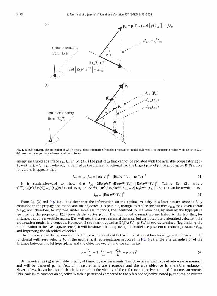
Fig. 1. (a) Objective pn the projection of which onto a plane originating from the propagation model E(b) results in the optimal velocity via distance dmin.

(b) Error on the objective and associated magnitudes.


energy measured at surface GH. Jres in Eq. (3) is the part of J0 that cannot be radiated with the available propagator E (b).By writing J0¼ Jattþ Jres, where Jatt is defined as the attained functional, i.e., the largest part of J0 that propagator E (b) is ableto radiate, it appears that:

Jatt ¼ J0�Jres ¼ :pðGHÞ:2�:EðbÞvoptðGsÞ�pðGHÞ:

2(4)

It is straightforward to show that Jatt ¼ 2ReðpnðGHÞEðbÞvoptðGsÞÞ�:EðbÞvoptðGsÞ:2. Taking Eq. (2), where

vopt*(Gs)(E*(b)E(b))¼p*(GH)E(b), and using 2ReðvoptnðGsÞE

nðbÞEðbÞvoptðGsÞÞ ¼ 2:EðbÞvoptðGsÞ:

2, Eq. (4) can be rewritten as

Jatt ¼ :EðbÞvoptðGsÞ:2

(5)

From Eq. (2) and Fig. 1(a), it is clear that the information on the optimal velocity in a least square sense is fullycontained in the propagation model and the objective. It is possible, though, to reduce the distance dmin for a given vectorp(GH), and, therefore, to improve, under some assumptions, the identified source velocities, by moving the hyperplanespanned by the propagator E(b) towards the vector p(GH). The mentioned assumptions are linked to the fact that, forinstance, a square invertible matrix E(b) will result in a zero minimal distance, but an inaccurately identified velocity if thepropagation model is erroneous. However, if the matrix equation E (b)v(Gs)¼p(GH) is overdetermined (legitimizing theminimization in the least square sense), it will be shown that improving the model is equivalent to reducing distance dmin

and improving the identified velocities.The efficiency F of the optimization is defined as the quotient between the attained functional Jatt and the value of the

functional with zero velocity J0. In the geometrical representation proposed in Fig. 1(a), angle c is an indicator of thedistance between model hyperplane and the objective vector, and we can write:

F ¼Jatt

J0¼ 1�

Jres

J0¼ 1�

d2min

J0¼ ðcoscÞ2 (6)

At the outset, p(GH) is available, usually obtained by measurements. This objective is said to be of reference or nominal,and will be denoted pn. In fact, all measurements are erroneous and the true objective is, therefore, unknown.Nevertheless, it can be argued that it is located in the vicinity of the reference objective obtained from measurements.This leads us to consider an objective which is perturbed compared to the reference objective, noted ~pn that can be written


as ~pn ¼ pnþdpn, where dpn is a perturbation of the reference objective. It should be emphasized that the true, exactobjective, which is inaccessible, will be considered as a perturbed field compared to the erroneous objective, which isaccessible and here called nominal or reference.

Such a perturbation may be characterized by a relative error eð ~pnÞ ¼ ð:pn� ~pn:Þ=:pn: which, in turn, may constitute avicinity around the reference field containing all the perturbed fields such that their relative error is less than or equal to agiven value of e. Ideally, to a definition of the vicinity around pn should correspond a vicinity around the efficiency F(pn),also written Fn, in order to establish a connection between efficiency and error on the objective and, by so doing, to be ableto see how the efficiency diverges from that of the reference field when the error on the latter increases. In fact, theprevious definition of the vicinity around pn expressed by e is such that to a given efficiency corresponds an infinitenumber of different values of e spread over the interval [e,þN(. Indeed, the efficiency defined by angle c – associated with~pn – is the same for an infinite number of collinear fields ~pn, and, therefore, to an infinite number of values of eð ~pnÞ. On thecontrary, for all these collinear fields sharing the same efficiency, a single minimum value can be defined [11]:

eminð ~pnÞ ¼:pn�ð ~p

n

npn=: ~pn:2

L2 Þ ~pn:

:pn:(7)

belonging to the interval [0,1]. Moreover, it has been shown, in another context [11], that to a given value of emin

corresponds a single value of the minimum guaranteed efficiency when the perturbed field ~pn belongs to the vicinitydefined by emin. It is straightforward to verify from Eq. (7) that all perturbed fields collinear to a perturbed field have thesame value of emin (i.e., ~pn and a ~pn where a is a complex scalar result in the same value of emin). In fact, Eq. (7) forparameter emin has a simple geometrical meaning: it is the norm of the difference between the reference objective pn andits projection (denoted ~p0n) on the perturbed objective ~pn, divided by the norm of the reference objective. In thegeometrical representation of Fig. 1(b), it is the sinus of angle y, necessarily between 0 and 1. Thus, parameter emin¼sin y isa measure of the aperture of the cone centered on the reference objective (Fig. 2(a)). Not only do all fields collinear to aperturbed field on the cone share the same value of emin, but also do all fields on the cone (the second assertion includesthe first). Moreover, all perturbed fields inside or on the cone are characterized by a minimal relative error less than orequal to that associated with the cone.

Fig. 2. (a) An error on the objective manifests itself by a cone centered on the reference objective and of aperture y and (b) the set of cone generatrices

gives rise to the cloud bounded by curves.

0.0 0.2 0.4 0.6 0.8 1.00

10

20

30

40

50

60

70

1

sin

sin

Fig. 3. (a) Geometrical representation when pn belongs to the model plane and (b) expected associated cloud.


A point of coordinates (eminð ~pnÞ, dminð ~p0

nÞ) can be associated to each perturbed field ~pn in the vicinity of the reference

field. For a set of perturbed fields sharing the same minimal relative error emin, the values dminminðeminÞ and dmax

min ðeminÞ bound

the range of dminð ~p0

nÞ for any field considered in that set (Fig. 2(a)). Furthermore, for all the fields ~pn with the same value

emin, we have : ~p0n:¼ Constant. In other words, for a given propagation model (here for a fixed value of b) and a given

reference objective pn, a cloud may be constructed from points associated with the perturbed fields, with coordinates

eminð ~pnÞ,ffiffiffiffiffiffiffiffiffiffiffiffiffiffiffiffiffiffiffiffiffiffiffiffiffiffiffiffiffiffiffiJ0ð ~pnÞ=Jresð ~pnÞ

p¼ : ~pn:=dminð ~pnÞ ¼ : ~p 0n:=dminð ~p

0

nÞ

� �, ranging between upper and lower boundaries, defined by

curves dminminðeminÞ and dmax

min ðeminÞ. Fig. 2(b) shows the upper and lower bounds of the cloud built from the inverse of minimal

distances as indicated. One should be aware of the fact that all points corresponding to fields with an error less than orequal to a given value of emin are located to the left of the vertical line at emin and between the two bounds.

If objective pn belongs to the model plane (Fig. 3(a)), a situation rarely, if ever, present, but which is sought, then c¼0

and dminðpnÞ ¼ 0. Moreover with a cone of aperture y centered on pn belonging to the model plane, one has

dminminðeminÞ ¼ dmax

min ðeminÞ as can be seen in Fig. 3(a) where only the projection of the cone to the plane perpendicular to

that of the model and containing the reference objective is shown. In this case the cloud shrinks to a single line (upper and

lower bounds merged) expressed as 1/sin y (Fig.3(b)). Indeed for a given value of emin there is one value of y and, by

definition, for the fields on the cone, dmin ¼ 1=siny.In order to show that the geometrical interpretation with its notions of cone and cloud is relevant, because it suggests

ways of improving the estimation of the propagator, a simple one-dimensional analytical example will be used in the nextsection. It will be seen that, as the shape of the cloud depends on the distance between model hyperplane and the objectivevector, it provides information about the model. It will also be shown that the quality of the holographic procedure may bequantitatively defined, as has already been done in another domain of acoustics [11].

3. Simple analytical example

The one dimensional simple example consisting of a duct with cross section of area S under plane wave propagationassumption chosen to illustrate the utility of the geometric representation, is defined in the semi-infinite domain [0,þN(.It is shown in Fig. 4. A source of strength q1 located at x1 constitutes the source to be identified from two measuredpressures pH1

and pH2measured at xH1

and xH2, respectively, making up the hologram. The artificial boundary condition is

expressed as an admittance at x¼0 and describe the ‘‘rear’’ acoustic radiation in the domain )�N,0] as well as possiblehidden sources in this domain. In the present example such a source is located at x2 and has the source strength q2.

In domain [0,þN( the radiated pressure is obtained classically by the superposition of the waves propagating in bothdirections to the right and left of the source at x1. The pressures may be computed analytically from the right-handmember of the Helmholtz equation related to a source of strength q1, the boundary condition at x¼0, the radiationcondition at infinity, the continuity of pressure and the jump of velocity at the source location x1. This results for x1a0 and

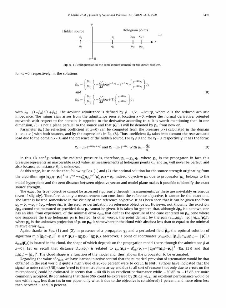
Fig. 4. 1D configuration in the semi-infinite domain for the direct problem.


for x1¼0, respectively, in the solutions

pH ¼pH1

pH2

( )¼rc

2SðR0 e�ikx1þeþ ikx1 Þ

e�ikxH1

e�ikxH2

( )q1

and

pH ¼pH1

pH2

( )¼rc

2SðR0þ1Þ

e�ikxH1

e�ikxH2

( )q1

(8)

with R0 ¼ 1�b0

� �= 1þb0

� �. The acoustic admittance is defined by b¼ 1=Z ¼�rcv=p, where Z is the reduced acoustic

impedance. The minus sign arises from the admittance seen at location x¼0, where the normal derivative, orientedoutwards with respect to the domain, is opposite to the derivative according to x. It is worth mentioning that, in onedimension, GH is not a plane parallel to the source and that p(GH) will be denoted by pH from now on.

Parameter R0 (the reflection coefficient at x¼0) can be computed from the pressure p(x) calculated in the domain)�N,þN( with both sources, and by the expressions in Eq. (8). Thus, coefficient R0 takes into account the rear acousticload due to the domain xo0 and the presence of the hidden source. For x1a0 and for x1¼0, respectively, it has the form:

R0 ¼ m0 e�ikðx1þx2Þ and R0 ¼ m0 e�ikx2 with m0 ¼q2

q1(9)

In this 1D configuration, the radiated pressure is, therefore, pH ¼ gb0q1, where gb0

is the propagator. In fact, thispressure represents an inaccessible exact value, as measurements at hologram points xH1

and xH2will never be perfect, and

also because admittance b0 is unknown.At this stage, let us notice that, following Eqs. (1) and (2), the optimal solution for the source strength originating from

the algorithm minq

:gb0q�pH:

2is qopt ¼ ðgn

b0gb0Þ�1ðgn

b0pHÞ ¼ q1. Indeed, objective pH due to propagator gb0

belongs to the

model hyperplane and the zero distance between objective vector and model plane makes it possible to identify the exactsource strength.

The exact (or true) objective cannot be accessed rigorously through measurements, as these are inevitably erroneous(even if slightly). Therefore, as only a measurement can constitute the reference objective, it cannot be the exact one.The latter is located somewhere in the vicinity of the reference objective. It has been seen that it can be given the formpH ¼ ~pn ¼ pnþdpn, where dpn is the error or perturbation on reference objective pn. However, not knowing the exact pH,dpn around the measured or provided data pn cannot be given. It is taken for granted that, although dpn is unknown, onehas an idea, from experience, of the minimal error emin that defines the aperture of the cone centered on pn, cone whereone supposes the true hologram pH is located. In other words, the point defined by the pair (eminðpHÞ, :p0H:=dminðp

0HÞ),

where p0H is the unknown projection of pn on pH, is somewhere in the cloud with abscissa less than or equal to the minimalrelative error emin.

Again, thanks to Eqs. (1) and (2), in presence of a propagator gb and a perturbed field ~pn, the optimal solution of

algorithm minq

:gbq� ~pn:2

is qoptð ~pnÞ ¼ ðgn

bgbÞ�1ðgn

b~pnÞ. Moreover, a point of coordinates (eminð ~pnÞ,: ~pn:=dminð ~pnÞ ¼ : ~p 0n:=

dminð ~p0

nÞ) is located in the cloud, the shape of which depends on the propagation model (here, through the admittance b at

x¼0). Let us recall that distance dminð ~p0

nÞ is related to Jresð ~pnÞ ¼ d2minð ~pnÞ ¼ :gbqoptð ~pnÞ� ~pn:

2(Eq. (3)) and that

J0ð ~pnÞ ¼ : ~pn:2. The cloud shape is a function of the model and, thus, allows the propagator to be estimated.

Regarding the value of emin, we have learned in active control that the numerical prevision of attenuation would be thatobtained in the real world if quite a high value of 20–30 percent were to occur. In NAH, authors have indicated that thesignal to noise ratio (SNR) transferred to the microphone array and due to all sort of reasons (not only due to errors on themicrophones) could be estimated. It seems that �40 dB is an excellent performance while �30 dB to �15 dB are morecommonly accepted. By considering that these SNR could be expressed by 20log10emin, an excellent performance would beone with a emin less than (as in our paper, only what is due to the objective is considered) 1 percent, and more often lessthan between 3 and 18 percent.


At this point, an important remark must be made. When, on the one hand, the model varies via the parameter R (or b, or

m in Eq. (9); the exact values are R0, b0 and m0) and when, on the other hand, the reference objective is the exact one, it canbe seen in the 1D configuration analyzed that the propagator gb remains collinear to gb0

, whatever the value of R (see

Eq. (8) where R gives rise to gb in p¼gbq1). From the geometrical interpretation, whatever b, the true objective pH (¼pn) islocated in the model plane and can be perfectly reached through a multiplicative coefficient, here a source strength. In

these conditions, dminmin ¼ dmax

min and the cloud calculated from various propagators always has the same shape as in Fig. 3(b).

In this particular situation, no information can be deduced from the cloud to guide the estimation of an improved model,here by estimating the admittance. For the geometrical interpretation to be helpful, the propagator must vary in a noncollinear way for the model hyperplane to move nearer to or farther from vector pn when the model parameters change. To

this end, the ratio of both components of vector gb, that is ðgbÞ2=ðgbÞ1, must vary with b. For this reason, in order to

approach the three dimensional case where geometrical wave damping exists independently of any dissipativephenomenon, a wave attenuation against the distance from the source was chosen in an arbitrarily and artificial way,

with dependence of the type 1=r 1=4. Thus, in the domain)�N,þN(, the pressure has the form:

pðxÞ ¼rc

2Sq1

1

9x�x191=4

e�ik9x�x19þm

x�x2j j1=4e�ik9x�x29

!(10)

Knowing that

pðxÞ ¼rc

2Sq1

1

ðx�x1Þ1=4

eþ ikx1þR1

ðx�x01Þ1=4

eþ ikx01

!e�ikx

in the 1D semi-infinite domain with x01 the image source location through the ‘‘mirror’’ at the origin, and with the receiverpoint upstream from both sources, it is straightforward to show that R can be expressed as

Rðx,x1,x2,mÞ ¼ m xþx1

x�x2

� �1=4

eikðx1þ x2Þ (11)

When p(x) is the exact value, the reflection coefficient R has the value R0, or m¼m0.It should be noted that to solve the direct problem in the semi-infinite 1D domain only the image source method is

valid. Indeed, calculation using wave propagation along increasing and decreasing x would lack clarity due to theattenuation increasing with distance from the source. Integral representation cannot be used here either, as no 1D operatorleading to an elementary solution with amplitude that decays with the power 1/4 from the source is known.

By comparing Eqs. (9) and (11), with an attenuation of the wave amplitude, coefficient R now depends not only on mand on the distance between the two sources, but also on the distances between receiver points and sources. DenotingR1 and R2 the values of R at xH1

and xH2, the new analytical forms of the radiated pressure, and, thus, of the propagator, are,

respectively,

pH1

pH2

( )¼

rc2S

1ðxH1�x1Þ

1=4 eþ ikx1þR11

ðxH1�x0

1Þ1=4 eþ ikx0

1

� �e�ikxH1

1ðxH2�x1Þ

1=4 eþ ikx1þR21

ðxH2�x0

1Þ1=4 eþ ikx0

1

� �e�ikxH2

8>>><>>>:

9>>>=>>>;

q1

and

ðgbÞ1

ðgbÞ2

( )¼

rc2S

1ðxH1�x1Þ

1=4 eþ ikx1þR11

ðxH1�x0

1Þ1=4 eþ ikx0

1

� �e�ikxH1

1ðxH2�x1Þ

1=4 eþ ikx1þR21

ðxH2�x0

1Þ1=4 eþ ikx0

1

� �e�ikxH2

8>>><>>>:

9>>>=>>>;

(12)

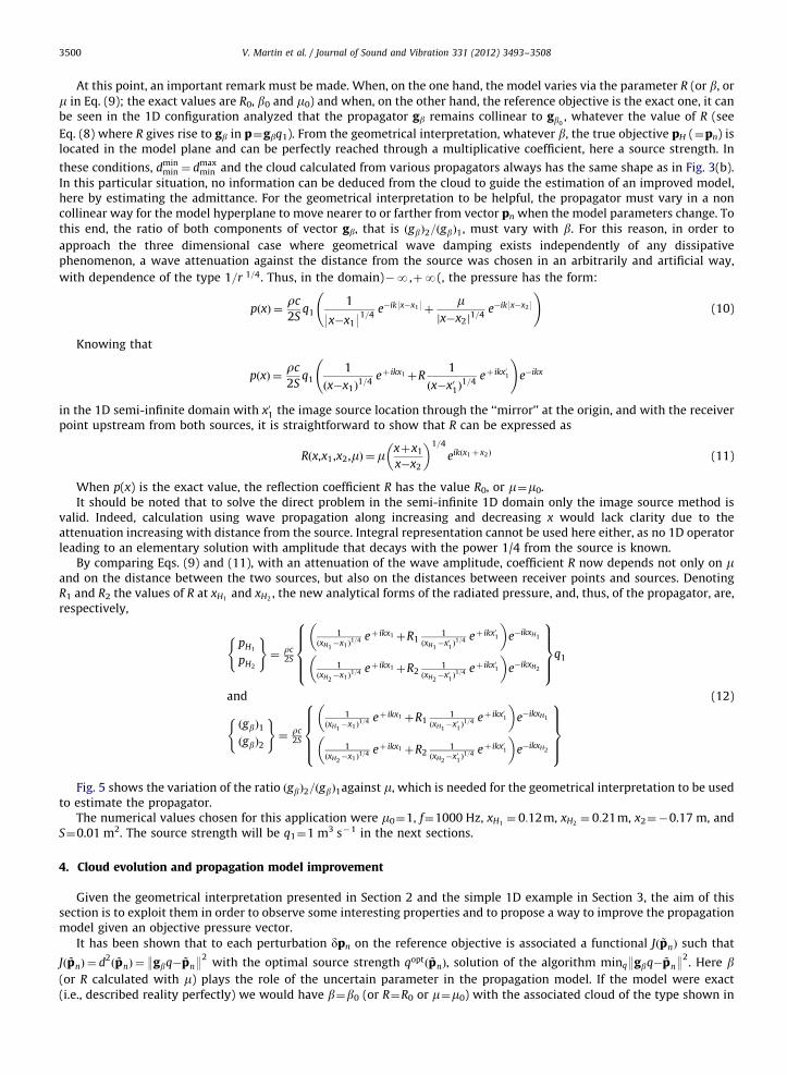
Fig. 5 shows the variation of the ratio ðgbÞ2=ðgbÞ1against m, which is needed for the geometrical interpretation to be usedto estimate the propagator.

The numerical values chosen for this application were m0¼1, f¼1000 Hz, xH1¼ 0:12m, xH2

¼ 0:21m, x2¼�0.17 m, andS¼0.01 m2. The source strength will be q1¼1 m3 s�1 in the next sections.

4. Cloud evolution and propagation model improvement

Given the geometrical interpretation presented in Section 2 and the simple 1D example in Section 3, the aim of thissection is to exploit them in order to observe some interesting properties and to propose a way to improve the propagationmodel given an objective pressure vector.

It has been shown that to each perturbation dpn on the reference objective is associated a functional Jð ~pnÞ such that

Jð ~pnÞ ¼ d2ð ~pnÞ ¼ :gbq� ~pn:

2with the optimal source strength qoptð ~pnÞ, solution of the algorithm minq:gbq� ~pn:

2. Here b

(or R calculated with m) plays the role of the uncertain parameter in the propagation model. If the model were exact

(i.e., described reality perfectly) we would have b¼b0 (or R¼R0 or m¼m0) with the associated cloud of the type shown in

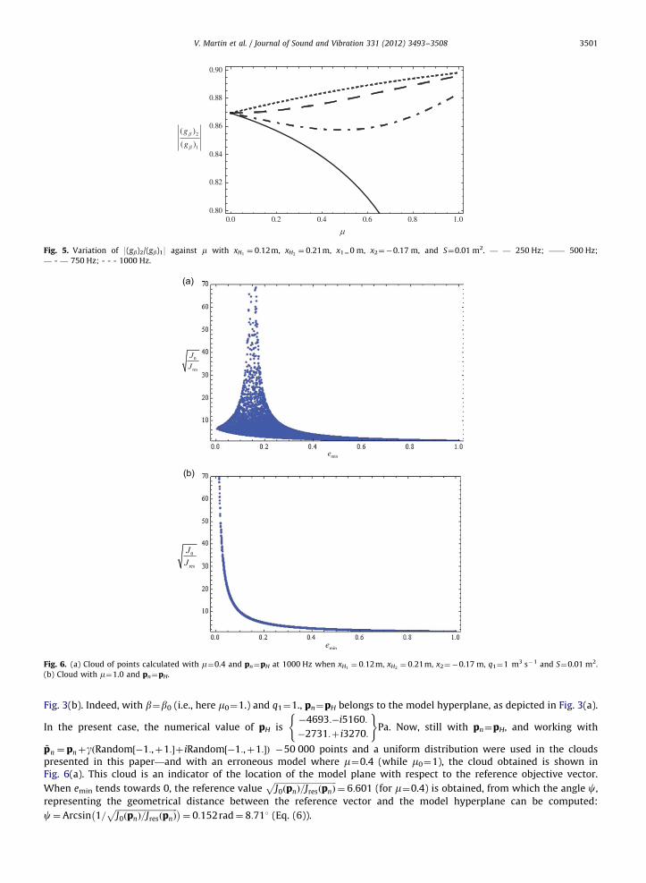
Fig. 6. (a) Cloud of points calculated with m¼0.4 and pn¼pH at 1000 Hz when xH1¼ 0:12m, xH2

¼ 0:21m, x2¼�0.17 m, q1¼1 m3 s�1 and S¼0.01 m2.

(b) Cloud with m¼1.0 and pn¼pH.

0.0 0.2 0.4 0.6 0.8 1.00.80

0.82

0.84

0.86

0.88

0.90

2

1

( )

( )

g

g

Fig. 5. Variation of 9(gb)2/(gb)19 against m with xH1¼ 0:12m, xH2

¼ 0:21m, x1¼0 m, x2¼�0.17 m, and S¼0.01 m2. — — 250 Hz; —— 500 Hz;

— - — 750 Hz; - - - 1000 Hz.


Fig. 3(b). Indeed, with b¼b0 (i.e., here m0¼1.) and q1¼1., pn¼pH belongs to the model hyperplane, as depicted in Fig. 3(a).

In the present case, the numerical value of pH is�4693:�i5160:

�2731:þ i3270:

( )Pa. Now, still with pn¼pH, and working with

~pn ¼ pnþgðRandom½�1:,þ1:�þ iRandom½�1:,þ1:�Þ �50 000 points and a uniform distribution were used in the cloudspresented in this paper—and with an erroneous model where m¼0.4 (while m0¼1), the cloud obtained is shown inFig. 6(a). This cloud is an indicator of the location of the model plane with respect to the reference objective vector.

When emin tends towards 0, the reference valueffiffiffiffiffiffiffiffiffiffiffiffiffiffiffiffiffiffiffiffiffiffiffiffiffiffiffiffiffiffiJ0ðpnÞ=JresðpnÞ

p¼ 6:601 (for m¼0.4) is obtained, from which the angle c,

representing the geometrical distance between the reference vector and the model hyperplane can be computed:

c¼ Arcsin 1=ffiffiffiffiffiffiffiffiffiffiffiffiffiffiffiffiffiffiffiffiffiffiffiffiffiffiffiffiffiffiJ0ðpnÞ=JresðpnÞ

p� �¼ 0:152rad¼ 8:711 (Eq. (6)).


It should be mentioned that there is a value eymin of emin such that y¼c, which is eymin ¼ sinc¼ 0:151 in the present case.

This value is related to the aperture of the error cone for which a generatrix belongs to the model plane (i.e., the cone is

tangent to this plane) and there is a perturbed field belonging to the cone such thatffiffiffiffiffiffiffiffiffiffiffiffiffiffiffiffiffiffiffiffiffiffiffiffiffiffiffiffiffiffiffiJ0ð ~pnÞ=Jresð ~pnÞ

pbecomes infinite

(Figs. 2(a) and (b) and 6(a)).For a given reference objective, the shape of the cloud varies when parameter m varies and modifies the propagator gb.

When m¼m0¼1, i.e., when the propagator gb is the exact model gb0, the cloud has the shape shown in Fig. 6(b), identical to

the expected one, shown in Fig. 3(b), resulting in the reference objective being located on the model plane. Table 1compares some of the information obtained from clouds in Figs. 6(a) and (b).

Now that we have illustrated with a simple example that the cloud changes with the model, we want to know how it

changes. To this end, two parameters closely related to the cloud form were chosen, namely c and eymin, to observe how they

change according to the model, here described through parameter m. Given an exact model (i.e. the exact value m0 of m) and the

perfect objective pn¼pH accompanying it, Figs. 7(a) and (b) show how c and eymin vary according to m. Three cases of an exact

model have been considered with m0 of value 1., or 0.8, or �0.3. Here, in order to be able to plot a simple 2D graph, m is a real

scalar (i.e., the two sources are in phase or out of phase). The values of eyminðmÞ are obtained by looking at the ‘‘highest’’ point in

the cloud and, even for a very large number of points in the cloud, the maximum value offfiffiffiffiffiffiffiffiffiffiffiffiffiffiffiffiffiffiffiffiffiffiffiffiffiffiffiffiffiffiJ0ð ~pnÞ=Jresð ~pnÞ

pis only an

approximation of what ought to be observed and, therefore, leads to the irregular curve in Fig. 7(b).

Table 1Comparison of data from Figs. 6(a) and (b).

Erroneous model with

m¼0.4

True model with

m0¼1.

Cloud of Fig. 6(a) Cloud of Fig. 6(b)

Angle c in radians 0.152 0ffiffiffiffiffiffiffiffiffiffiffiffiffiffiffiffiJ0ðpnÞ

JresðpnÞ

sfor emin ¼ 0

6.601 N

Angle y such that ( ~pnwithffiffiffiffiffiffiffiffiffiffiffiffiffiffiffiffiffiffiffiffiffiffiffiffiffiffiffiffiffiffiffiJ0ð ~pnÞ=Jresð ~pnÞ

p-1 0.152 0

Fig. 7. (a) c and (b) eymin, against m for various values of m0 at 1000 Hz when xH1¼ 0:12m, xH2

¼ 0:21m, x2¼�0.17 m, q1¼1 m3 s�1 and S¼0.01 m2.

Table 2Summary of results shown in Figs. 7(a) and (b).

Value of m Property of c(m) and of eminðmÞ

-7N -an asymptote, function of m0

1.2 -maximal value 8m0

m0 0 8m0


When m¼m0, the model is co-planar, presently collinear, with the reference objective, and eymin ¼c¼ 0. It should benoted that, in the present configuration, the functions of m are analytical. When m moves away from m0 (m positive ornegative), it appears that eymin and c converge towards a same horizontal asymptote. Indeed, when the modulus of mincreases, according to Eqs. (11) and (12), the propagator gb becomes

mrc

2Seikx2

1ðxH1�x2Þ

1=4 e�ikxH1

1ðxH2�x2Þ

1=4 e�ikxH2

8><>:

9>=>;

and, whatever m, all the propagators are collinear, with the consequence that the model plane is no longer modified byparameter m. Physically speaking, for m-7N, the reflection coefficient R has the same value.

Besides, whatever m0, it is remarkable that the values of m leading to a maximum value of eymin or c are identical withvalue m¼1.2. No straightforward explanation has been found so far, but it is noted that the scalar ðgn

b gbÞ�1 is maximal at

m¼1.2, which is probably at the origin of the maximum of Jresð ~pnÞ=J0ð ~pnÞ whatever m0. However no conclusion can bedrawn easily, due to the norm of a product of a matrix by a vector. From a geometrical point of view, one could expect amaximal angle of 901 for c and a maximal value of 1 for eymin. It is likely that constraining the ratio m to be real does notallow reaching this theoretical maximum angle. Nevertheless, this does not explain the apparent independence seen onthe graphs of the maximal values with regard to m0. Table 2 summarizes the results in Figs. 7(a) and (b). It should bementioned that plotting c(m) is also possible when parameter m is a complex scalar, with a three dimensional plot ofcðReðmÞ,ImðmÞÞ. However, these plots are not worth presenting here, as they are less clear than Fig. 7.

A similar study has been carried out using three and four points for the hologram. The clouds so obtained lead to thesame conclusion as that originating from a hologram with two points. Thanks to the observed evolution of the parameterscharacterizing the cloud, it is possible to define an algorithm, in particular by looking to the value of m that minimizes theangle c and, by so doing, reach the exact value m0, i.e. the exact model.

At this stage, the cloud notion is not absolutely necessary to improve the model, the minimal distance being sufficient.However, the notion of cloud is fundamental for the next step, to be presented in the next section.

In this section two main points have to be emphasized. First, that the properties of the clouds obtained from purelyspeculative thought based upon a geometrical representation were actually observed and have been shown to havephysical meaning in the case of a simple analytical example of an inverse acoustical problem, representative of a moregeneral case. Second, it was shown to be possible to make the cloud shape to come closer to the optimal shape shown inFig. 3(b), by adapting a model parameter. In the next section it will be shown that this step is the first to be taken in orderto be able to assess quantitatively the quality of the inverse acoustic procedure.

5. Guaranteed quality and required accuracy of the propagator

Having previously emphasized the relevance of the geometrical representation for inverse acoustic methods such asNAH and for improving the propagation model, a quality measure of the procedure will now be defined. It will be shownthat it is possible to guarantee a minimum quality in the presence of errors in the hologram. Moreover, it will be shownthat there is a limit to the accuracy of the propagator beyond which any improvement will be inefficient, as the quality ofthe inverse process will not be significantly enhanced.

For a given reference objective pn, the reference or nominal quality is defined by the quantity:

Qn ¼

ffiffiffiffiffiffiffiffiffiffiffiffiffiffiffiffiffiffiJ0ðpnÞ

d2minðpnÞ

sor Q2

n ¼1

1�Fnor Qn ¼

1

sinc(13)

with Fn defined in Eq. (6) (and d2minðpnÞ ¼ JresðpnÞ). It is observed that the reference quality is best (Qn¼þN) when

d2minðpnÞ ¼ 0, i.e., when the objective is situated on the plane associated with the propagation model (cf. Fig. 3(a)) and it is

worst (Qn¼1) when d2minðpnÞ ¼ J0ðpnÞ, i.e., the objective is orthogonal to the model plane. In active noise control, when one

considers pH¼pn, Qn is related to the obtained attenuation.Now, let us envisage a perturbation on the exact objective (i.e., with pH ¼ ~pnapn) such that it has a minimal error of

less than or equal to a value emin. Geometrically speaking, this means that, as seen in Fig. 2(a), the true hologram is locatedsomewhere close to the measured one, in or on the cone centered on the reference objective pn and of aperture angle y.If, in the geometrical representation, p0max

H is the projection of the hologram on the edge of the cone located farthest from


the model plane, the holographic procedure quality for the true hologram is always better than that defined by

Qg ¼

ffiffiffiffiffiffiffiffiffiffiffiffiffiffiffiffiffiffiffiffiffiffiffiffiJ0ðp

0maxH Þ

d2minðp

0maxH Þ

s(14)

said to be of minimum or guaranteed quality (Figs. 1(b) and 2(a) are useful here). It should be noticed, also, that the bestquality is accompanied by a cloud shape as the one in Fig. 3(b), while the poorest is also associated with a particular cloud.

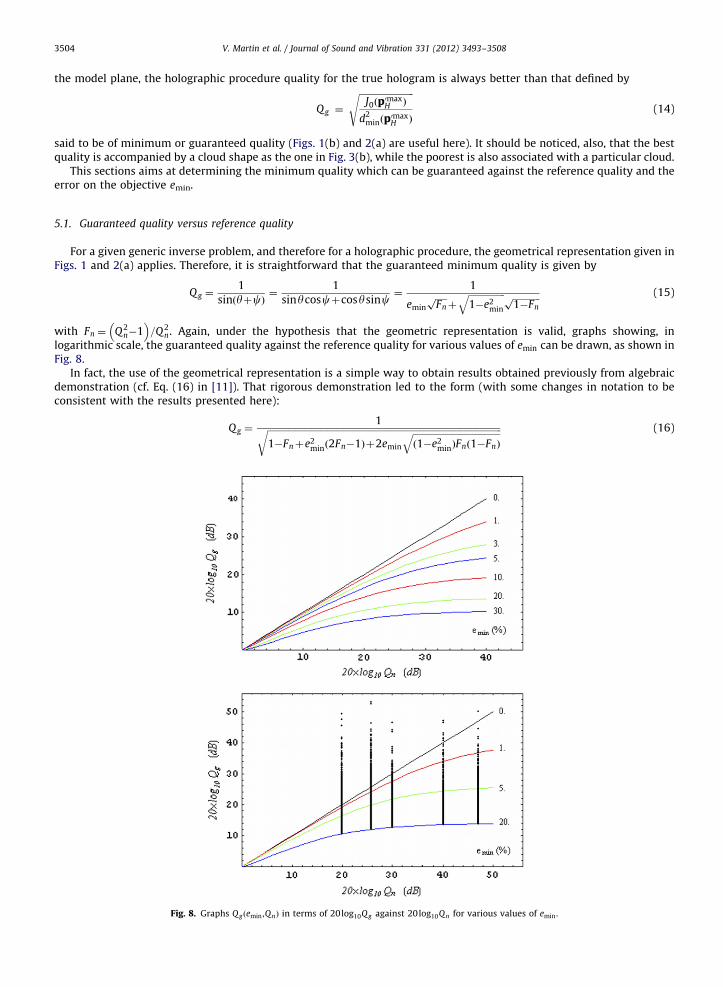
This sections aims at determining the minimum quality which can be guaranteed against the reference quality and theerror on the objective emin.

5.1. Guaranteed quality versus reference quality

For a given generic inverse problem, and therefore for a holographic procedure, the geometrical representation given inFigs. 1 and 2(a) applies. Therefore, it is straightforward that the guaranteed minimum quality is given by

Qg ¼1

sinðyþcÞ¼

1

sinycoscþcosysinc¼

1

emin

ffiffiffiffiffiFn

pþ

ffiffiffiffiffiffiffiffiffiffiffiffiffiffiffiffi1�e2

min

q ffiffiffiffiffiffiffiffiffiffiffiffi1�Fn

p (15)

with Fn ¼ Q2n�1

� �=Q2

n. Again, under the hypothesis that the geometric representation is valid, graphs showing, inlogarithmic scale, the guaranteed quality against the reference quality for various values of emin can be drawn, as shown inFig. 8.

In fact, the use of the geometrical representation is a simple way to obtain results obtained previously from algebraicdemonstration (cf. Eq. (16) in [11]). That rigorous demonstration led to the form (with some changes in notation to beconsistent with the results presented here):

Qg ¼1ffiffiffiffiffiffiffiffiffiffiffiffiffiffiffiffiffiffiffiffiffiffiffiffiffiffiffiffiffiffiffiffiffiffiffiffiffiffiffiffiffiffiffiffiffiffiffiffiffiffiffiffiffiffiffiffiffiffiffiffiffiffiffiffiffiffiffiffiffiffiffiffiffiffiffiffiffiffiffiffiffiffiffiffiffiffiffiffiffiffiffiffiffiffiffiffiffiffiffiffiffiffi

1�Fnþe2minð2Fn�1Þþ2emin

ffiffiffiffiffiffiffiffiffiffiffiffiffiffiffiffiffiffiffiffiffiffiffiffiffiffiffiffiffiffiffiffiffiffiffiffiffiffið1�e2

minÞFnð1�FnÞ

qr (16)

Fig. 8. Graphs Q gðemin ,QnÞ in terms of 20log10Qg against 20log10Qn for various values of emin.


which can be shown to be exactly Eq. (15) as the denominator of Eq. (16) can be written

ð1�FnÞð1�e2minÞþe2

minFnþ2emin

ffiffiffiffiffiffiffiffiffiffiffiffiffiffiffiffiffiffiffiffiffiffiffiffiffiffiffiffiffiffiffiffiffiffiffiffiffiffið1�e2

minÞFnð1�FnÞ

q� �1=2

orffiffiffiffiffiffiffiffiffiffiffiffiffiffiffiffiffiffiffiffiffiffiffiffiffiffiffiffiffiffiffiffiffiffið1�FnÞð1�e2

minÞ

qþemin

ffiffiffiffiffiFn

p� �2 !1=2

which is the denominator of Eq. (15). From this perfect equivalence, a new and more relevant expression, this time general,for Eq. (16) of [11] is therefore Eq. (15). Without the geometrical interpretation this form could not have been guessed.

Under these conditions, the graphs of Fig. 8 are strictly the same as those of Fig. 6 in [11]. They indicate that, for anyhologram presenting a minimal error relative to the reference of less than or equal to emin, the quantity Qg truly constitutesthe guaranteed quality (in terms of objective reached by the inverse procedure).

5.2. Consequences on the required accuracy of the propagation model

Graphs Qgðemin,QnÞ in logarithmic scale (dB) reveal that the curves tend towards a plateau when the reference quality isimproved, with an effect which becomes increasingly visible as error emin increases. The plateau when Qn-N, i.e., whenangle c-0, has the value Qg ¼ 1=siny. In Fig. 8 we see that in the presence of an error of emin ¼ 20 percent, the guaranteedquality stagnates around 12 dB as soon as the reference quality exceeds 30 dB. It is thus useless to look for a modelestimator leading to a reference quality of over 30 dB. In geometrical terms, there is no point in asking the model to benearer to the reference objective beyond a certain distance. This remark is essential, as it provides an indication of the levelof propagation model accuracy in the presence of a given minimal error on the hologram.

Let us note that the guaranteed quality is obtained from a given cone centered on pn and for a given reference quality(thus for a given model). The measured and therefore inaccurate objective could perhaps have been made nearer the trueobjective pH by removing part of the noise included in pn with the consequence of making the cone to which pH belongsnarrower (i.e., by decreasing emin or the angle y). Within this possibly reduced cone, the guaranteed quality has beendefined from the objective vector on the cone the farthest from the model hyperplane without any consideration of thephysical sense. The field in the subset of physical fields on and in the cone may make it possible to improve the guaranteedquality further by looking at the field of the subset the farthest from the model hyperplane. Let us imagine some orders ofmagnitude. Let us suppose a signal to noise ratio of �15 dB at the microphone array and due only to noise on the referenceobjective pn. It corresponds to a value emin of 18 percent and let us consider 20 dB for Qn. Removing some noise, the SNRdiminishes as does emin to reach, for example, 10 percent. In fact by so doing we have introduced a modified pmodif

n nearerto pH. Moreover pmodif

n more physically acceptable is likely to be nearer the hyper model plane leading to a better Qmodifn

(reference quality) say 28 dB instead of 20 dB. Already the guaranteed quality would be Qmodifg ¼ 18dB instead of Qg¼10 dB

(see Fig. 8). Finally, looking for only the physically acceptable fields could still improve Qmodifg . It is therefore clear that the

guaranteed quality defined in this paper as the worst quality could be improved if we are able to remove some noise fromthe reference objective and if we are able to define a subset of physical fields in or on the cone.

5.3. Numerical application to the 1D simple example

To illustrate the previously mentioned properties using the simple 1D problem presented in Section 3, an exacthologram and a reference hologram playing the role of a measured one are computed from the propagation model. Thevalue of eminðpn,pHÞ (depending on the reference and the true holograms) is thus accessible and the cone including the truehologram pH can be defined. Moreover, we are in a position to look for an estimate gb of the model as close as possible tothe reference hologram. From this knowledge, the reference quality Qn(pn,gb) follows (Eq. (13)). According to the proximityof the model to the reference pressure vector, the various reference qualities obtained can now be located on variouspoints on the abscissa axis of graphs in Fig. 8.

A large number of perturbed holograms ~pn are computed from random variations (additive uniform distribution)around the reference hologram pn. The error eminðpn, ~pnÞ is calculated for each ~pn. From the numerous values (samples) of~pn, all those with a minimal error less than or equal to a given value emin, larger than eminðpn,pHÞ, are extracted. Underthese conditions, the cone related to emin includes the true hologram pH. For each of these selected holograms, the qualityQ of the holography procedure is calculated. Finally, the relation Q ZQgðemin,QnÞ is verified directly on the graph in Fig. 8.

For the parameter values in Section 3, the numerical value of the perfect objective is pH ¼�4693�i5160

�2731þ i3270

( )Pa.

Arbitrarily, the perturbation is chosen as dp¼�178�i1547

�701þ i1551

( )Pa resulting in a reference hologram pn ¼

�4516�i3613

�2030þ i1720

( )Pa and eminðpn,pHÞ ¼ 18 percent.

Improvement of the propagation model by adapting parameter m (chosen as a real value at this stage) so that the modelplane comes closer to the reference objective (let us recall that the true objective pH is not accessible and, therefore,no model improvement can be made to come closer to pH) leads to m¼1.05 (different from m0¼1). With this estimatedpropagation model one obtains

ffiffiffiffiffiFn

p¼ 0:987. For such a value of

ffiffiffiffiffiFn

pcorresponding to an angle cE91 and a reference


quality of Qn¼6, the best model obtained for real values of m is not excellent as would be the case for co21, norunsatisfactory as it has been the case for c4101. These values of the angle arise from our experience in the capacity inreconstructing a satisfactory velocity in numerical holography as given in Table 5 of [13]. In this numerical application,Fig. 7(a) becomes Figs. 9(a) and 2(b) becomes Fig. 9(b). The cloud of points is quite different from the ideal cloud ofFig. 3(b), which would be obtained if the model hyperplane had included pn.

In practice, let us suppose that the pressure pH of the true hologram is located in a cone centered on the measured(reference) pressure pn, the aperture of which is related to emin ¼ 20 percent. It is now known that it is pointless to look fora model of a quality, relative to the reference hologram, greater than 30 dB, since the guaranteed quality will not besignificantly better than 12 dB. Having found a model gb with a 30 dB quality, the quality of the holographic procedureassociated to pH with model gb may be, say, of 42 dB, perhaps, say, of 12.5 dB, but definitely not less than 12 dB.

Before ending this section, it should be emphasized that the quality of the holographic procedure in no way defines thequality of the identified source strength (or surface velocities) obtained through holography (or another inverse acoustictechnique). The latter constitutes a different problem and a subject for further investigation, possibly using the geometricalinterpretation, but which will require other considerations than the error cone proposed here. As a preliminaryinvestigation, Figs. 10(a) and (b) show how the identified source strength tends towards the exact value when the modeltends towards the exact model, as the reference hologram tends towards the exact one. Fig. 10(a) was obtained withpHapn. To each value of c (or of Fn, or of m, now a complex scalar) corresponds a set of optimal values qopt of the sourcestrength (actually a complex scalar, only the real part being shown on the figure), of which the existence can beunderstood via the geometrical representation. It is also noticed that various values of c may lead to a same value qopt.Here, again, the geometrical representation helps to understand why this is so, but in a less straightforward way. Thus,points in Fig. 10(a) do not give direct information, but the cloud envelope actually converges towards a single value of thesource strength when c-0 (variation of c in the interval from 01 to 51 allows the convergence to be seen clearly).Fig. 10(b) corresponds to pH¼pn. Both figures help to see how the identified source strength converges towards the truevalue when the estimated model and the measured hologram become the true ones. How to master this convergence is asubject for further investigation with the aim of defining the quality of the identified velocity (or source strength) in thepresence of errors on the hologram and the propagation model.

This section has covered five main points. First, for a given propagator corresponds a definition of the quality of theholographic process in the reference or nominal situation. Second, by considering the error on the hologram, a guaranteed

0.0 0.2 0.4 0.6 0.8 1.00

10

20

30

40

50

60

70

Fig. 9. (a) Evolution of angle c against parameter m and (b) cloud of points calculated with optimal parameter m (m¼1.05) and pnapH.

Fig. 10. (a) Real part of the identified source strength against the proximity of the model to the reference hologram different from the true hologram.

(b) Real part of the identified source strength against the proximity of the model to the reference hologram identical to the true hologram.


quality can be obtained. Third, when the propagator plane comes closer to the vector of the reference hologram, the qualityin the reference situation increases. Fourth, in presence of errors in the objective, there is no need to go too far inimproving the propagator, as improving the propagator may not allow to insure better quality past a certain quality limit(an excellent propagator is not necessarily much better than a good one on the presence of measurement errors). Finally,even if the quality of the holographic process is not directly related to the quality of the identified source strength(or surface velocities), convergence towards good estimated source strength values is observed when the propagator tendstowards the true one.

6. Conclusions

Following a geometrical representation previously proposed in the context of active noise control [11], thisrepresentation is applied in the framework of inverse acoustic problems such as NAH. To illustrate the proposed approach,a 1D elementary acoustic source identification problem easily described analytically, but somehow including some of theeffects found in more complex 3D problems, has been used. It has been shown that the geometrical interpretation can beapplied in this new context and appears to be an efficient tool for defining the quality of the holographic procedure, inparticular for establishing a guaranteed quality.

When the model can be improved (by estimating, in the present case, some unknown parameters linked to boundaryconditions), as long as a relatively small difference between the measured hologram and the exact one (i.e., without anymeasurement error) is expected, the estimated model can be reasonably close to the true one, which is also inaccessible inthe real world.

It is supposed that the exact hologram is in the vicinity of the measured one, the vicinity being geometrically describedas the domain inside a cone centered on the available (reference) hologram, interpreted as a vector. The aperture of thecone is directly linked to the estimated or given error between the two holograms (measurement error). From among allthe holograms contained in or on the cone, one will lead to the worst case regarding holography quality. Such informationprovides a way of quantifying the quality which can be guaranteed.


Despite the fact that the quality of the holographic procedure is not a direct indicator of the quality of the identifiedvelocity or source strength, it has been shown through numerical simulation how the identified source strength tendstowards the true source strength when the error on the measured hologram decreases, i.e., when the estimated modeltends towards the true one.

The proposed method is expected to face two main difficulties when applied to complex 3D problems. First, previousworks have shown that, when dealing with a 3D direct problem, the admittance on the area containing the visiblevibrating area can vary greatly [10]. Improving the propagation model via these boundary conditions would be difficult.A preliminary work would consist, therefore, in obtaining functions to describe the spatial dependence of admittancedepending on a small number of parameters. Second, in the geometrical representation, the very gradual variation in themodel plane with the variation of the admittance observed in the elementary 1D example will certainly disappear whendealing with complex 3D problems. Should an optimization method be used, such as a genetic algorithm, the inevitableproblem of the computation time needed to converge would be an issue.

Whatever the type of variation of the model plane with the boundary conditions, the search for a good estimator of thepropagation model is a non-convex optimization problem. Only by implementing the global procedure on a 3D model will theanswers be found. If the model is accessible within a reasonable computational time, it is expected that quantifying the qualitywill be possible. Some of these questions have already received an affirmative answer in the case of a vibrating disk [13].

Finally, the approach presented in this paper is suitable for over-determined harmonic problems where the objective isgiven. The adaptation of an intrinsic model parameter could be extended to the dimension of the model as long as theproblem remains over-determined but there is also a limitation in presence of errors in the objective. For the time being,the geometrical approach cannot deal with under-determined problems, nor with problems where the dimension of theobjective varies, nor with time-domain holography.

Acknowledgments

The authors thank the Agence de l’Environnement et de la Maıtrise d’Energie (ADEME) in France for funding this studywithin the framework of the REBECA 0566c0073 research project.

References

[1] J.D. Maynard, E.G. Williams, Y. Lee, Nearfield Acoustic Holography; I. Theory of generalized holography and the development of NAH, Journal of theAcoustical Society of America 78 (4) (1985) 1395–1412.

[2] W.A. Veronesi, J.D. Maynard, Nearfield Acoustic Holography (NAH); II. Holographic reconstruction algorithms and computer implementation, Journalof the Acoustical Society of America 81 (5) (1987) 1307–1322.

[3] E.G. Williams, G. Earl, Fourier Acoustics, Sound Radiation and Nearfield Acoustical Holography, Academic Press, 1999.[4] Y. Kim, P.A. Nelson, Estimation of acoustic source strength within a cylindrical duct by inverse methods, Journal of Sound and Vibration 275 (2004)

391–413.[5] M.R. Bai, Application of BEM (boundary element method)-based acoustic holography to radiation analysis of sound sources with arbitrarily shaped

geometries, Journal of the Acoustical Society of America 92 (1992) 199–209.[6] Z. Zhang, N. Vlahopoulos, S.T. Raveendra, T. Hallen, K.Y. Zhang, A computational acoustic field reconstruction process based on an indirect boundary

element formulation, Journal of the Acoustical Society of America 108 (2000) 199–209.[7] X. Zhao, S.F. Wu, Reconstruction of vibro-acoustic fields using hybrid nearfield acoustic holography, Journal of Sound and Vibration 282 (2005)

1183–1199.[8] S.F. Wu, Hybrid near-field acoustic holography, Journal of the Acoustical Society of America 115 (2004) 207–217.[9] P.C. Hansen, Rank-deficient and Discrete Ill-posed Problems, SIAM, 1998.

[10] V. Martin, T. Le Bourdon, Acoustic holography and complementary boundary conditions, Proceedings of the Congress ICSV14, Cairns, Australia, 2007.[11] V. Martin, C. Gronier, Minimum attenuation guaranteed by an active noise control system in presence of errors in the spatial distribution of the

primary field, Journal of Sound and Vibration 217 (5) (1998) 827–852.[12] V. Martin, How accurate are results obtained by acoustic holography? Proceedings of the Congress Novem05, Saint-Raphael, France, 2005.[13] V. Martin, T. Le Bourdon, A.M. Pasqual, Numerical simulation of acoustic holography with propagator adaptation, application to a 3D disc, Journal of

Sound and Vibration 330 (2011) 4233–4249.

Geometrical interpretation of acoustic holography: Adaptation of the propagator and minimum quality...

Documents

Transcript of Geometrical interpretation of acoustic holography: Adaptation of the propagator and minimum quality...