Geometric nonlinearity -...
88
Computational Mechanics, AAU, Esbjerg Nonlinear FEM Course in Nonlinear FEM Geometric nonlinearity
Transcript of Geometric nonlinearity -...

Computational Mechanics, AAU, EsbjergNonlinear FEM
Course inNonlinear FEM
Geometric nonlinearity

Geometric nonlinearity 2Computational Mechanics, AAU, EsbjergNonlinear FEM
Outline
Lecture 1 – IntroductionLecture 2 – Geometric nonlinearityLecture 3 – Material nonlinearityLecture 4 – Material nonlinearity continuedLecture 5 – Geometric nonlinearity revisitedLecture 6 – Issues in nonlinear FEALecture 7 – Contact nonlinearityLecture 8 – Contact nonlinearity continuedLecture 9 – DynamicsLecture 10 – Dynamics continued

Geometric nonlinearity 3Computational Mechanics, AAU, EsbjergNonlinear FEM
Nonlinear FEMLecture 1 – Introduction, Cook [17.1]:
– Types of nonlinear problems– Definitions
Lecture 2 – Geometric nonlinearity, Cook [17.10, 18.1-18.6]:– Linear buckling or eigen buckling– Prestress and stress stiffening– Nonlinear buckling and imperfections– Solution methods
Lecture 3 – Material nonlinearity, Cook [17.3, 17.4]:– Plasticity systems– Yield criteria
Lecture 4 – Material nonlinearity revisited, Cook [17.6, 17.2]:– Flow rules– Hardening rules– Tangent stiffness

Geometric nonlinearity 4Computational Mechanics, AAU, EsbjergNonlinear FEM
Nonlinear FEMLecture 5 – Geometric nonlinearity revisited, Cook [17.9, 17.3-17.4]:
- The incremental equation of equilibrium- The nonlinear strain-displacement matrix- The tangent-stiffness matrix- Strain measures
Lecture 6 – Issues in nonlinear FEA, Cook [17.2, 17.9-17.10]:– Solution methods and strategies– Convergence and stop criteria– Postprocessing/Results– Troubleshooting

Geometric nonlinearity 5Computational Mechanics, AAU, EsbjergNonlinear FEM
Nonlinear FEMLecture 7 – Contact nonlinearity, Cook [17.8]:
– Contact applications– Contact kinematics– Contact algorithms
Lecture 8 – Contact nonlinearity continued, Cook [17.8]:– Issues in FE contact analysis/troubleshooting
Lecture 9 – Dynamics, Cook [11.1-11.5]:– Solution methods– Implicit methods– Explicit methods
Lecture 10 – Dynamics continued, Cook [11.11-11.18]:– Dynamic problems and models– Damping– Issues in FE dynamic analysis/troubleshooting

Geometric nonlinearity 6Computational Mechanics, AAU, EsbjergNonlinear FEM
Typical Nonlinear Problem1 D-O-F
u
P
k
ukk
kkk
N
0
N0
of functionconstant+=

Geometric nonlinearity 7Computational Mechanics, AAU, EsbjergNonlinear FEM
( ))u(fk
Pukk
N
N
=
=+0
Given P find u. Assume f(u) is a known function.
Problem Statement
Geometric nonlinearity 8Computational Mechanics, AAU, EsbjergNonlinear FEM
Slope k0
(kN = 0)HardeningkN > 0
SofteningkN < 0
u
P

Geometric nonlinearity 9Computational Mechanics, AAU, EsbjergNonlinear FEM
Definitions - PSTRES vs. SSTIFThe difference between PSTRES and SSTIF?
• SSTIF and PSTRES are essentially the same in what they do (calculate stress stiffness matrix). SSTIF triggers nonlinear equilibrium iterations, however, so this is where they differ.
• PSTRESSolve [K]x = FCalculate and store [Kσ](this means that "x" is solved for based on [K] only)
• SSTIFSolve [K]*x = FCalculate and store [Kσ]Solve [K+Kσ]*x=Fiterate until force equilibrium is satisfied(this means that "x" and corresponding stresses are based on updated [K+Kσ])
• Although both PSTRES and SSTIF calculate [Kσ], the latter triggers nonlinear equilibrium iterations, so that probably is where your difference in results lies.

Geometric nonlinearity 10Computational Mechanics, AAU, EsbjergNonlinear FEM
Definitions• Stress stiffening (only) - Strains and rigid-body motions are assumed
to be small, and stiffening (or softening) of the structure due to the stress state is taken into account.
• Stress stiffening is needed for structures which are thin in one (or two) dimensions (e.g., bending stiffness of beams and shells small compared with in-plane/transverse stiffness) since a coupling between the two occurs (examples - membrane of a drum or a guitar string).
• It is also needed when doing other types of analyses like buckling or modal where the stress state affects the response of the system.
• In ANSYS, stress stiffening terms are constant, so be aware of this assumption (since in prestress modal or eigenvalue buckling, analyses are linear too).

Geometric nonlinearity 11Computational Mechanics, AAU, EsbjergNonlinear FEM
Definitions• Stress stiffening may also be known as geometric stiffness matrix,
differential stiffness matrix, stability coefficient matrix, initial stress stiffness matrix, incremental stiff matrix, etc.
• Note that the commands SSTIF and PSTRES essentially do the same thing, but are used in different situations (PSTRES is used to request that a stress-stiffening matrix be written for use in a future eigenvalue buckling or pre-stressed modal analysis).
• For the 18x family of elements, stress-stiffening is not available independent of large deflection. For other elements, the decision to include stress-stiffening with large deflection is generally based on ease of convergence, since large deflection and stress-stiffening are redundant.

Geometric nonlinearity 12Computational Mechanics, AAU, EsbjergNonlinear FEM
DefinitionsConsistent Tangent Stiffness Matrix (CTS Matrix, for short)• Matrix used in nonlinear problems which is comprised of
– the "main tangent stiffness matrix" (the "regular" stiffness matrix we think of, especially in linear analyses),
– the "initial displacement matrix" (accounts for shape changes inelements),
– the "initial stress matrix" (the stress stiffening matrix; stiffness due to stress state), and
– the "initial load matrix" (stiffness associated with change in follower force loads during deformation - pressure load stiffness for elements 154/181/188/189).
– The 181/188/189 elements always use a fully consistent tangent stiffness matrix. The rest of the 18x family of elements does include a stress stiffening matrix, but not necessarily a fully CTS matrix.
Geometric nonlinearity 13Computational Mechanics, AAU, EsbjergNonlinear FEM
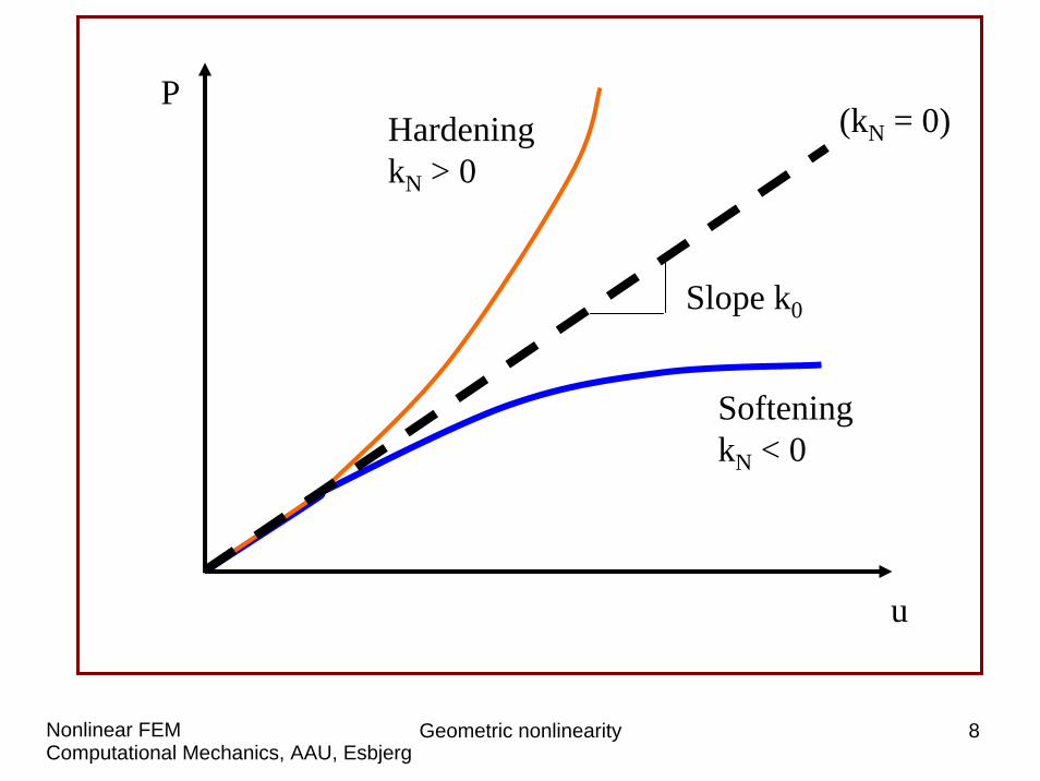
Definitions• Hierarchy of terms:
– finite strain (or large strain) – large deformation (or large rotation) – stress stiffening (there's also spin softening, which is not discussed here) – regular linear analysis
• So (1) encompasses (2)-(4), (2) encompasses (3)-(4), etc. This may be a bit of an oversimplification, but it may help to think of it in these terms. When SSTIF is not ON with NLGEOM,ON, it just leads to slower convergence; but that effect is included in the overall response/results (again, thin beams and shells may be exceptions).
• Note that, if you use NLGEOM,ON, SSTIF,ON will automatically be activated (at least for v5.5 and above). The defaults should be left alone (i.e., you do not need to manually activate SSTIF,ON). SSTIF,ON helps aid convergence, especially for thin beams and shells. Although it has no effect for the 18x elements, as noted above, it's just good practice to leave the defaults (i.e, default is SSTIF,ON when NLGEOM is ON)
Geometric nonlinearity 14Computational Mechanics, AAU, EsbjergNonlinear FEM
Objectives
1. Review buckling theory2. Eigenvector/value calculation3. FE Buckling analysis
Geometric nonlinearity 15Computational Mechanics, AAU, EsbjergNonlinear FEM
What is buckling?
• An element under compression will have different mechanical responses relating to the following factors:– Length vs cross-sectional dimensions– Eccentricity of loads– Applied load– etc
Geometric nonlinearity 16Computational Mechanics, AAU, EsbjergNonlinear FEM
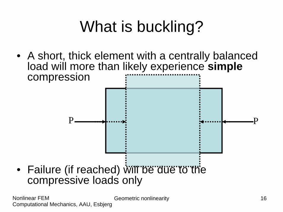
What is buckling?
• A short, thick element with a centrally balanced load will more than likely experience simplecompression
• Failure (if reached) will be due to the compressive loads only
PP

Geometric nonlinearity 17Computational Mechanics, AAU, EsbjergNonlinear FEM
What is buckling?
• A thin member under high and/or eccentric loads is more likely to deflect in a different manner – it will buckle IF the loading reaches a critical value (Pcr)

Geometric nonlinearity 18Computational Mechanics, AAU, EsbjergNonlinear FEM
What is buckling?
• The eccentric loading and/or small imperfections in the material cause out of line displacement
PcrPcr
L
Geometric nonlinearity 19Computational Mechanics, AAU, EsbjergNonlinear FEM
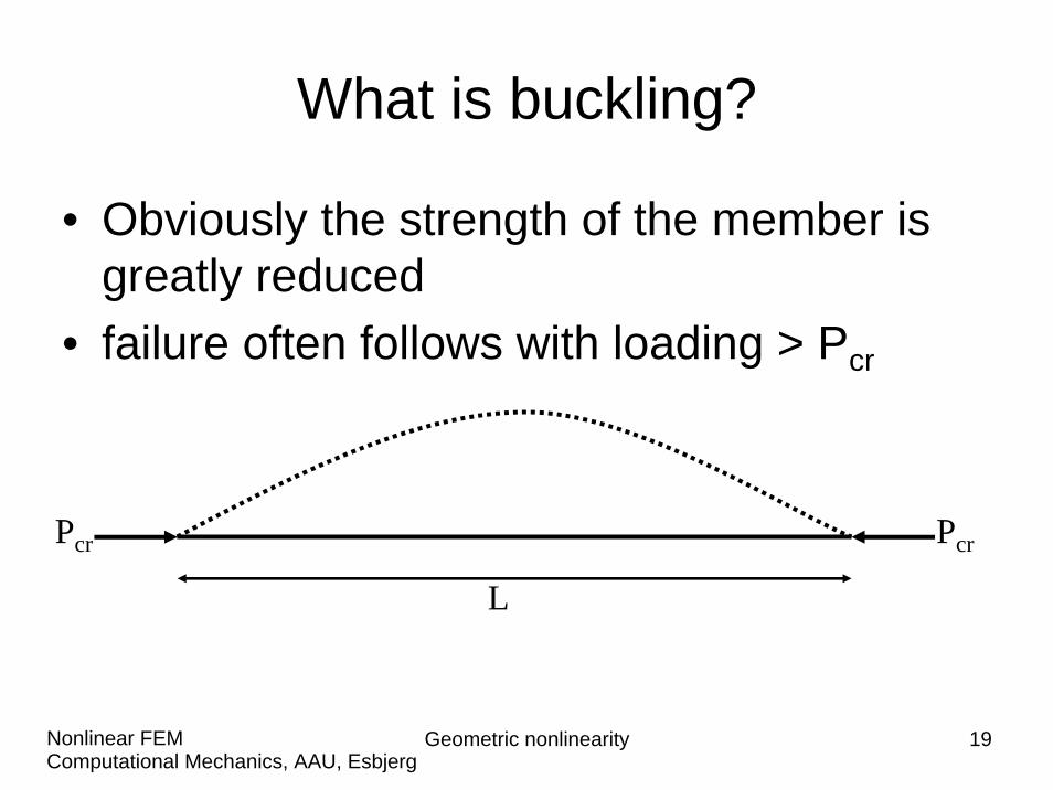
What is buckling?
• Obviously the strength of the member is greatly reduced
• failure often follows with loading > Pcr
PcrPcr
L

Geometric nonlinearity 20Computational Mechanics, AAU, EsbjergNonlinear FEM
Euler columns
• Basic analysis of circular columns with pinned ends
• Assuming the element bends towards the positive direction – the resultant moment is the negative of load x distance:
M = - Py

Geometric nonlinearity 21Computational Mechanics, AAU, EsbjergNonlinear FEM
Euler columns
• From basic beam theory
• Which has the simple solution:
yEIP
dxyd
EIM
2
2
−==
0yEIP
dxyd2
2
=+⇒
xEIPcosBx
EIPsinAy +=

Geometric nonlinearity 22Computational Mechanics, AAU, EsbjergNonlinear FEM
Euler columns
• Applying the boundary conditionsy = 0 at x = 0 and at x = L
• Therefore B = 0• We have the trivial solution A= 0• But otherwise
0xEIPsin =

Geometric nonlinearity 23Computational Mechanics, AAU, EsbjergNonlinear FEM
Euler columns
• Giving:
• Where N is an integer• Therefore we have discrete solutions to
the problem – similar shapes to harmonics in a guitar string
π= NLEIP
Geometric nonlinearity 24Computational Mechanics, AAU, EsbjergNonlinear FEM
Euler columns
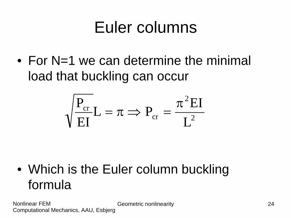
• For N=1 we can determine the minimal load that buckling can occur
• Which is the Euler column buckling formula
2
2
crcr
LEIPL
EIP π
=⇒π=

Geometric nonlinearity 25Computational Mechanics, AAU, EsbjergNonlinear FEM
Euler columns
• Looking at the deflection (y)
• Which is half of the sine curve:LxsinAy π
=
PcrPcr
L

Geometric nonlinearity 26Computational Mechanics, AAU, EsbjergNonlinear FEM
Euler columns
• From this simple example we can see that multiple (though discrete) solutions can be possible for a certain geometry and loading direction.
• Loading above the critical load could lead to buckling with higher order shapes (N>1)
• This means that the “steady state”problems we have been considering could bifurcate if loading is slightly changed

Geometric nonlinearity 27Computational Mechanics, AAU, EsbjergNonlinear FEM
Boundary conditions (BC’s)
• Boundary conditions will affect the shape significantly:
F F F

Geometric nonlinearity 28Computational Mechanics, AAU, EsbjergNonlinear FEM
Eigenvectors/values
• Just before looking at the FE formulation of buckling – the eigenvector analysis is revised
• If a problem can be written in the following form:
KU = λU– for scalar (eigenvalue) λ– Matrix K (n x n)– Eigenvector U = U1, U2, … Un

Geometric nonlinearity 29Computational Mechanics, AAU, EsbjergNonlinear FEM
Eigenvectors/values
• Re-arrangingKU-λU = 0
• Expanding the matrix (e.g. 2 x 2 matrix)
⎥⎦
⎤⎢⎣
⎡=⎥
⎦
⎤⎢⎣
⎡λ−⎥
⎦
⎤⎢⎣
⎡⎥⎦
⎤⎢⎣
⎡00
uu
uu
kkkk
2
1
2
1
2221
1211
⎥⎦
⎤⎢⎣
⎡=⎥
⎦
⎤⎢⎣
⎡⎥⎦
⎤⎢⎣
⎡λ−
λ−00
uu
kkkk
2
1
2221
1211
Geometric nonlinearity 30Computational Mechanics, AAU, EsbjergNonlinear FEM
Eigenvectors/values
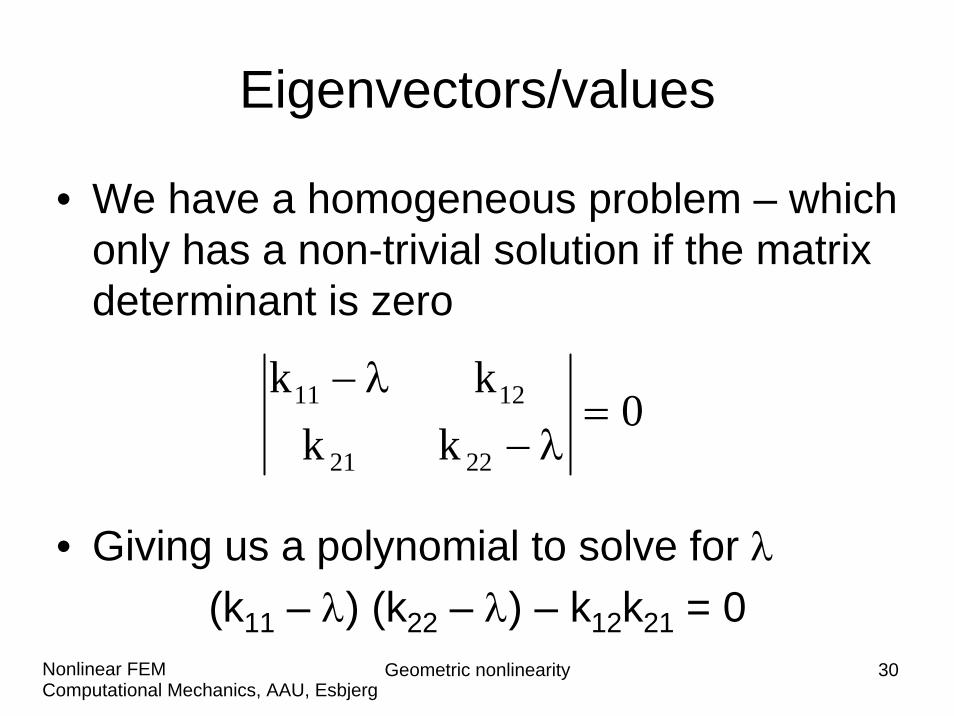
• We have a homogeneous problem – which only has a non-trivial solution if the matrix determinant is zero
• Giving us a polynomial to solve for λ(k11 – λ) (k22 – λ) – k12k21 = 0
0kk
kk
2221
1211 =λ−
λ−
Geometric nonlinearity 31Computational Mechanics, AAU, EsbjergNonlinear FEM
Eigenvectors/values
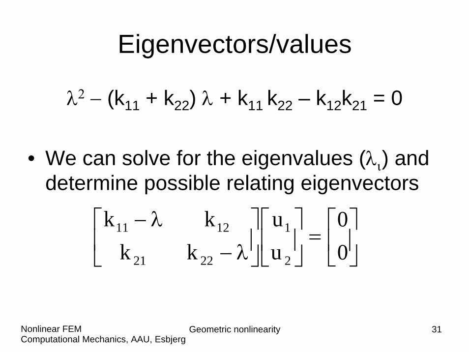
λ2 − (k11 + k22) λ + k11 k22 – k12k21 = 0
• We can solve for the eigenvalues (λι) and determine possible relating eigenvectors
⎥⎦
⎤⎢⎣
⎡=⎥
⎦
⎤⎢⎣
⎡⎥⎦
⎤⎢⎣
⎡λ−
λ−00
uu
kkkk
2
1
2221
1211

Geometric nonlinearity 32Computational Mechanics, AAU, EsbjergNonlinear FEM
FE Formulation
• Of course there are more complex theories of buckling but we will look at a discrete element and then a FE formulation
• As with the previous example, we need to assume there will be out of line deflection
• We either start with a slight bend (as before) or introduce a small force (or displacement) in a direction that will induce the desired deflection

Geometric nonlinearity 33Computational Mechanics, AAU, EsbjergNonlinear FEM
FE Formulation
• Consider the following idealisation of a column under a compressive load. The springs represent the “desire” of the structure to retain its shape.
F k
kkT
F
Rigid bars
L
L

Geometric nonlinearity 34Computational Mechanics, AAU, EsbjergNonlinear FEM
FE Formulation
• Consider the following idealisation of a column under a compressive load. The springs represent the “desire” of the structure to retain its shape.
k
kkT
F F
F
kU1
kU2
kU1+ kU2
Force Equilibrium

Geometric nonlinearity 35Computational Mechanics, AAU, EsbjergNonlinear FEM
FE Formulation
• Consider the following idealisation of a column under a compressive load. The springs represent the “desire” of the structure to retain its shape.
FkU1+ kU2
F
α
β
kTα

Geometric nonlinearity 36Computational Mechanics, AAU, EsbjergNonlinear FEM
FE Formulation
• Moment equilibrium of the bottom bar gives:
FLsin(β) + kTα = kU1Lcos(β)• Moment equilibrium about the centreFL[sin(β) + sin(β+α)] =
kU1L[cos(β)+cos(α+β) + kU2Lcos(β)• Assuming that displacements are small
we can relate Lsin(…) to U1 and U2

Geometric nonlinearity 37Computational Mechanics, AAU, EsbjergNonlinear FEM
FE Formulation
• Giving the following matrix:
• Now this is not of the form KU = λU BUT is still classified as an eigenvalue problem if both square matrices are symmetric
⎥⎦
⎤⎢⎣
⎡⎥⎦
⎤⎢⎣
⎡−
−=⎥
⎦
⎤⎢⎣
⎡
⎥⎥⎥
⎦
⎤
⎢⎢⎢
⎣
⎡
+−
−+
2
1
2
1
rr
rr
uu
2111
Fuu
Lk4kL
Lk2
Lk2
LkkL

Geometric nonlinearity 38Computational Mechanics, AAU, EsbjergNonlinear FEM
FE Formulation
• Giving the following matrix:
• Solving for the lowest eigenvalue F1 will give the critical load
⎥⎦
⎤⎢⎣
⎡⎥⎦
⎤⎢⎣
⎡−
−=⎥
⎦
⎤⎢⎣
⎡
⎥⎥⎥
⎦
⎤
⎢⎢⎢
⎣
⎡
+−
−+
2
1
2
1
rr
rr
uu
2111
Fuu
Lk4kL
Lk2
Lk2
LkkL

Geometric nonlinearity 39Computational Mechanics, AAU, EsbjergNonlinear FEM
FE Formulation
• FE Beam formulation:F
βFWe introduce a linear perturbation (βF) and look at the change in stiffness and loading on the structure using nonlinear analysis

Geometric nonlinearity 40Computational Mechanics, AAU, EsbjergNonlinear FEM
FE Formulation
• FE Beam formulation:F
βF As the structure deforms it is assumed that the stiffness of the structure is a linear function of those of previous iterations. For time τ:
τK = t-ΔtK + λ(tK - t-ΔtK)

Geometric nonlinearity 41Computational Mechanics, AAU, EsbjergNonlinear FEM
FE Formulation
• FE Beam formulation:F
βF •For non zero vectors υτKυ = 0
this tangent stiffness is singular due to the buckling
•Therefore:t-ΔtKυ = λ(t-ΔtK - tK)υ
•Where υ are the possible buckling modes of the problem
Geometric nonlinearity 42Computational Mechanics, AAU, EsbjergNonlinear FEM
FE Formulation
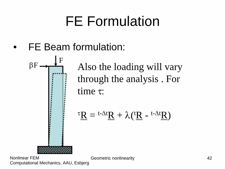
• FE Beam formulation:F
βF Also the loading will vary through the analysis . For time τ:
τR = t-ΔtR + λ(tR - t-ΔtR)

Geometric nonlinearity 43Computational Mechanics, AAU, EsbjergNonlinear FEM
FE Formulation
• Therefore we have eigenvalue problems to solve for each step of the iteration.
• If we choose a value of β that is sufficiently small then results will be very close to those predicted by the Euler column formula.
• The nonlinear iteration method will be introduced further later.

Geometric nonlinearity 44Computational Mechanics, AAU, EsbjergNonlinear FEM
Buckling Summary
• Buckling in structure? (eccentricity of loading, thin/thick, material imperfections)
• Simple beams under a buckling load can be analysed with Euler’s theory
• Rigid bar formulation leading to eigenvalueproblem
• Introduced the FE formulation of a linear perturbation giving eigenvalue problems for each iteration.
Geometric nonlinearityComputational Mechanics, AAU, EsbjergNonlinear FEM
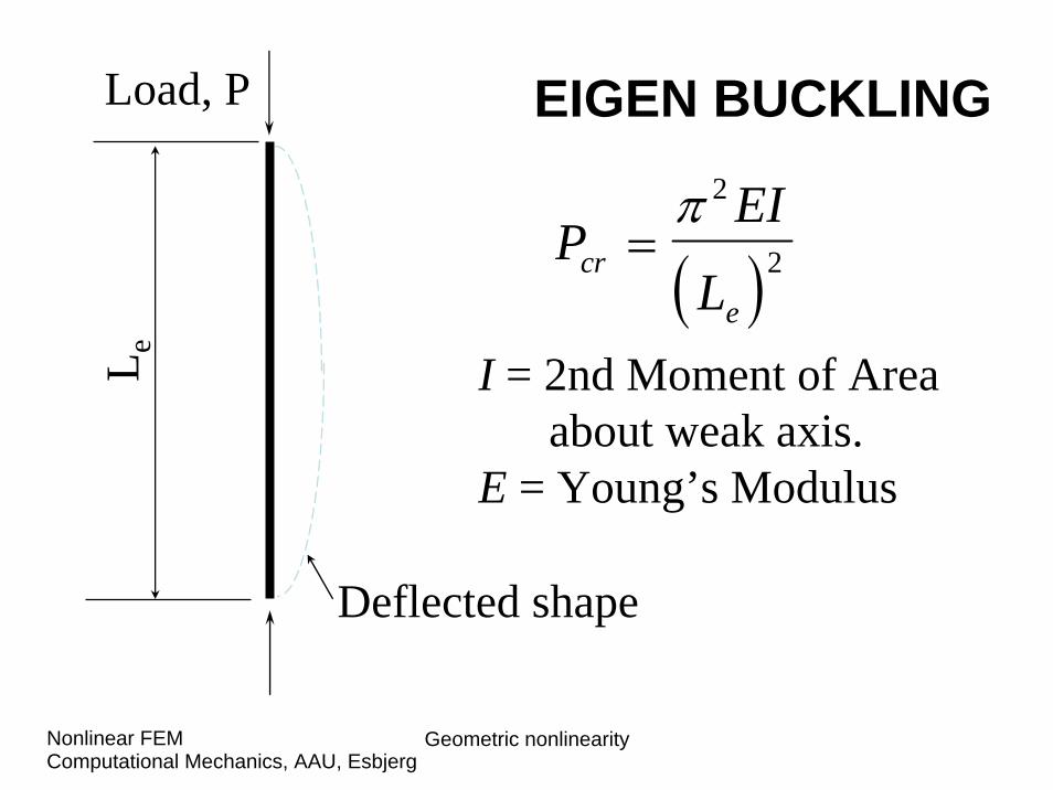
Load, P
Deflected shape
( )P
EI
Lcr
e
=π 2
2
L e I = 2nd Moment of Areaabout weak axis.
E = Young’s Modulus
EIGEN BUCKLING

Geometric nonlinearityComputational Mechanics, AAU, EsbjergNonlinear FEM
The effective length, Le, depends on the Boundary Conditions:

Geometric nonlinearityComputational Mechanics, AAU, EsbjergNonlinear FEM
Find the Buckling load for a pin-ended aluminumcolumn 3m high, with a rectangular x-section as
shown:P
P
50 mm
100 mm
Weak axis:Iyy = 100 (50)3/12
= 1.04x106 mm4
( )P
xcr =
π 2 6
2
72000 104 103000
( )( . )
= 82246 N

Geometric nonlinearity 48Computational Mechanics, AAU, EsbjergNonlinear FEM
Elastic Buckling Prediction• Numerical Methods
– finite element, finite strip (www.ce.jhu.edu/bschafer)• Hand Methods (for use in a traditional
Specification)– Local Buckling
• Element methods, e.g. k=4• Semi-empirical methods that include element interaction
– Distortional Buckling• Proposed (Schafer) method, rotational stiffness at web/flange
juncture• Hancock’s method• AISI (k for Edge Stiffened Elements per Spec. section B4.2)

Geometric nonlinearity 49Computational Mechanics, AAU, EsbjergNonlinear FEM
Elastic Buckling Comparisons1
(fcr)true = local or distoritonal buckling stress from finite strip analysis(fcr)element = minimum local buckling stress of the web, flange and lip via Eq.'s 1-3(fcr)interact = minimum local buckling stress using the semi-empirical equations (Eq.'s 4-6)(fcr)Schafer = distortional buckling stress via Eq.'s 7-15(fcr)Hancock = distortional buckling stress via Lau and Hancock (1987)(fcr)AISI = buckling stress for an edge stiffened element via AISI (1996) from Desmond et al. (1981)
Local Distortional (fcr)true (fcr)true (fcr)true (fcr)true (fcr)true
(fcr)element (fcr)interact (fcr)Schafer (fcr)Hancock (fcr)AISIAll Data avg. 1.34 1.03 0.93 0.96 0.79
st.dev. 0.13 0.06 0.05 0.06 0.33max 1.49 1.15 1.07 1.08 1.45min 0.96 0.78 0.81 0.83 0.18
count 149 149 89 89 89
*
*For members with slender webs and small flanges the Lau and Hancock (1987) approach conservatively converges to a buckling stress of zero (these members are ignored in the summary statistics given above)
1 For a wide variety of cold-formed steel lipped channels, zees and racks

Geometric nonlinearity 50Computational Mechanics, AAU, EsbjergNonlinear FEM
Effective Width Methods
⎟⎟⎠
⎞⎜⎜⎝
⎛⎟⎟⎠
⎞⎜⎜⎝
⎛−=
ff
ff
22.01b
b crcreff for 673.0ff
cr> , else bbeff = . (17)
where: beff is the effective width of an element with gross width b f is the yield stress (f = fy) when interaction with other modes is
not considered, otherwise f is the limiting stress of a modeinteracting with local buckling
crf is the local buckling stress
∑= tbA effeff
*
* for Euler (long column) interaction f=Fcr of the column curve used in AISC Spec.(the notation for f is Fn in the AISI Spec. but the same column curve is employed)

Geometric nonlinearity 51Computational Mechanics, AAU, EsbjergNonlinear FEM
Direct Strength Methods
4.cr
4.crn
PP
PP
15.01P
P⎟⎟⎠
⎞⎜⎜⎝
⎛⎟⎟
⎠
⎞
⎜⎜
⎝
⎛⎟⎟⎠
⎞⎜⎜⎝
⎛−= for 776.0
PP
cr> , else Pn = P . (19)
where: Pn is the nominal capacity P is the squash load (P = Py = Agfy) except when interaction with
other modes is considered, then P = Agf, where f is the limiting stress of the interacting mode.
crP is the critical elastic local buckling load (Ag crf )
6.
crd6.
crdn
PP
PP
25.01PP
⎟⎟⎠
⎞⎜⎜⎝
⎛
⎟⎟⎟
⎠
⎞
⎜⎜⎜
⎝
⎛
⎟⎟⎠
⎞⎜⎜⎝
⎛−= for 561.0
PP
crd> , else Pn = P. (16)
where: Pn is the nominal capacity in distortional buckling P is the squash load (P = Py = Agfy) when interaction with other
modes is not considered, otherwise P = Agf, where f is the limiting stress of a mode that may interact
Pcrd is the critical elastic distortional buckling load (Agfcrd)
Distortional
Local
Geometric nonlinearity 52Computational Mechanics, AAU, EsbjergNonlinear FEM
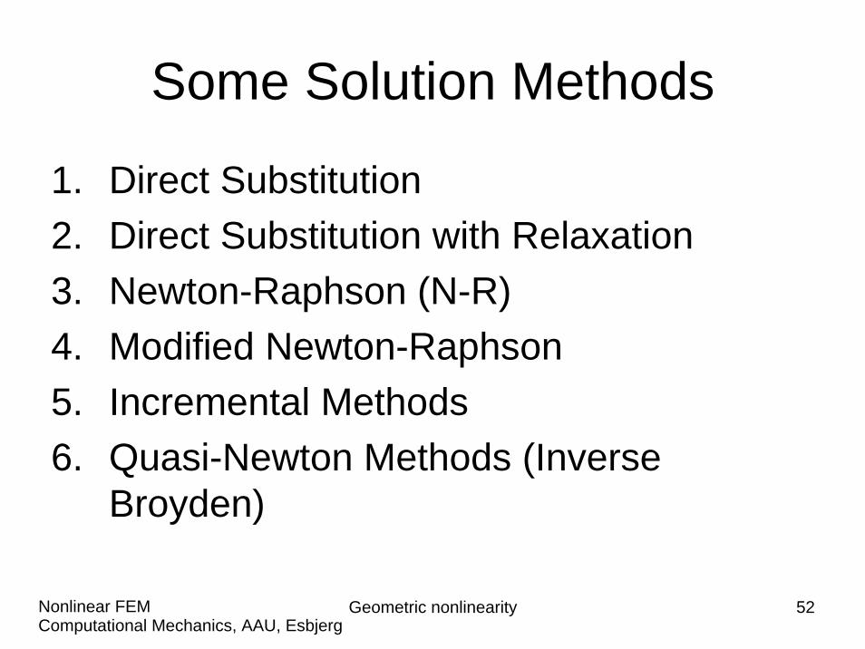
Some Solution Methods
1. Direct Substitution2. Direct Substitution with Relaxation3. Newton-Raphson (N-R)4. Modified Newton-Raphson5. Incremental Methods6. Quasi-Newton Methods (Inverse
Broyden)
Geometric nonlinearity 53Computational Mechanics, AAU, EsbjergNonlinear FEM
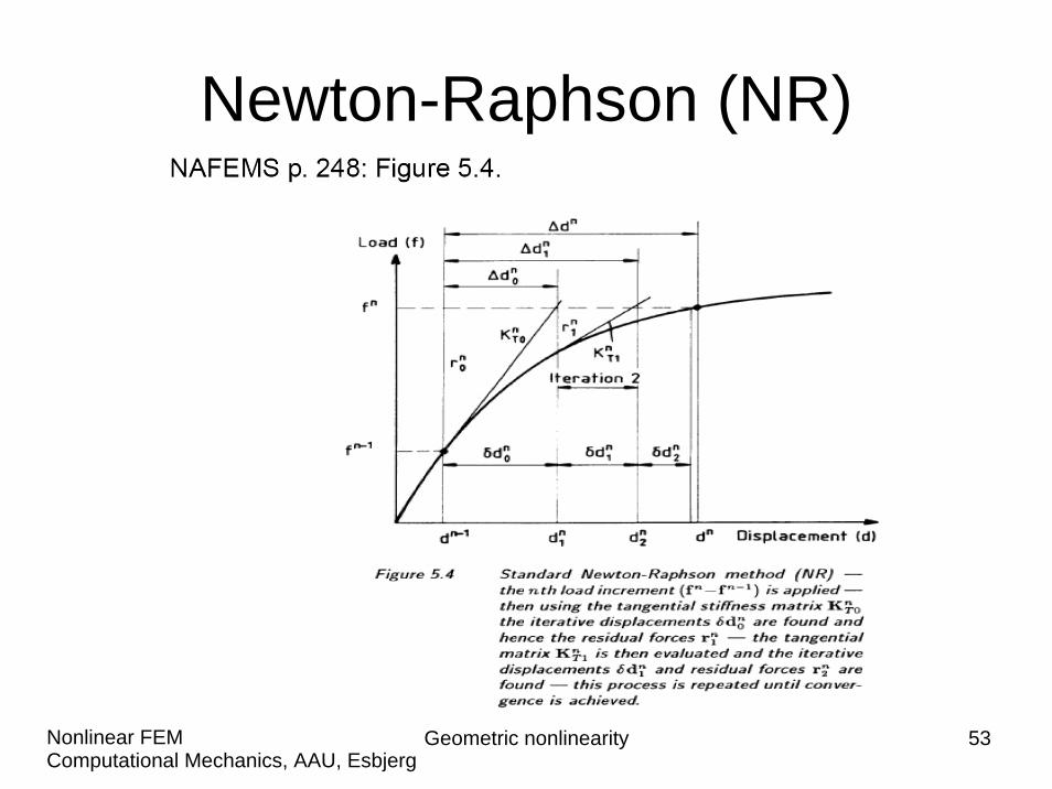
Newton-Raphson (NR)
Geometric nonlinearity 54Computational Mechanics, AAU, EsbjergNonlinear FEM
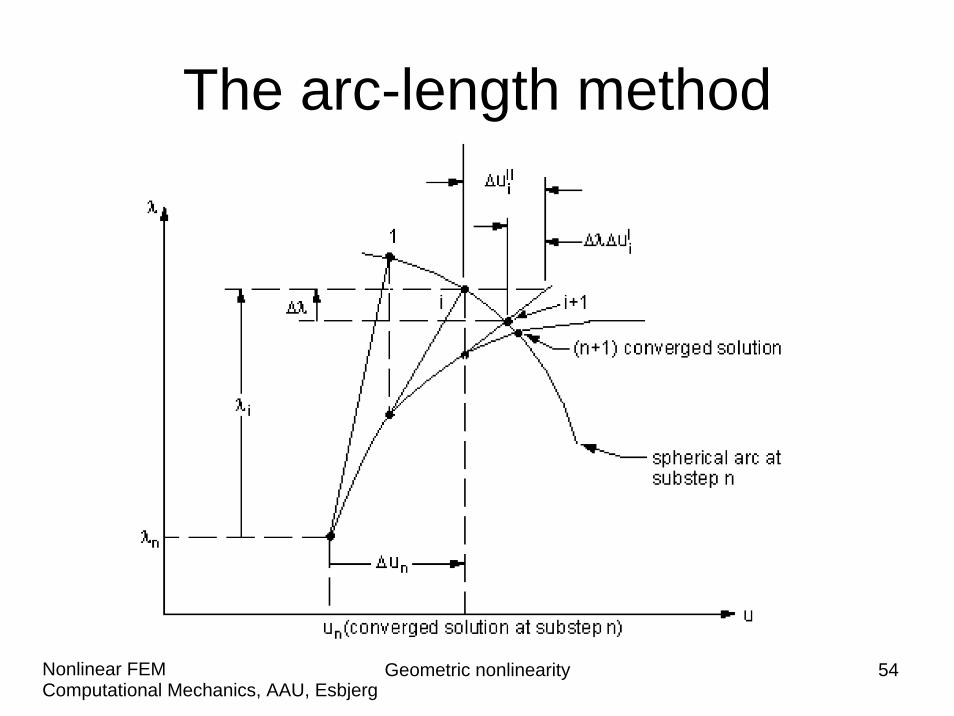
The arc-length method

Geometric nonlinearity 55Computational Mechanics, AAU, EsbjergNonlinear FEM
Direct Substitution Method1. Let load PA be applied to a softening spring (kN<0)2. Assume kN = 0 for the first iteration. 3. Compute first approximation to displacement: u1 =
PA/k0
4. Use u1 to compute new stiffness: k = k0 +f(u1)
5. Compute next approximation to displacement: u2 = PA/k
6. Generate sequence of approximations.

Geometric nonlinearity 56Computational Mechanics, AAU, EsbjergNonlinear FEM
( )( )
( ) ANi
AN
AN
A
Pkku
Pkku
Pkku
Pku
i
101
103
102
101
2
1
−
+
−
−
−
+=
+=
+=
=
Sequence of Operations

Geometric nonlinearity 57Computational Mechanics, AAU, EsbjergNonlinear FEM
u
P
PA
u1
k0
a
1P1

Geometric nonlinearity 58Computational Mechanics, AAU, EsbjergNonlinear FEM
u
P
PA
u1
k0
a
1
b
2
u2
k0+kN1
Essentially a secant method

Geometric nonlinearity 59Computational Mechanics, AAU, EsbjergNonlinear FEM
u
P
PA
u1
a
1
b
2
u2
c
3
u3

Geometric nonlinearity 60Computational Mechanics, AAU, EsbjergNonlinear FEM
u
P
PA
u1
a
1
b
2
u2
c
3
u3 uA

Geometric nonlinearity 61Computational Mechanics, AAU, EsbjergNonlinear FEM
1
006020
u.P
u.k=
−=
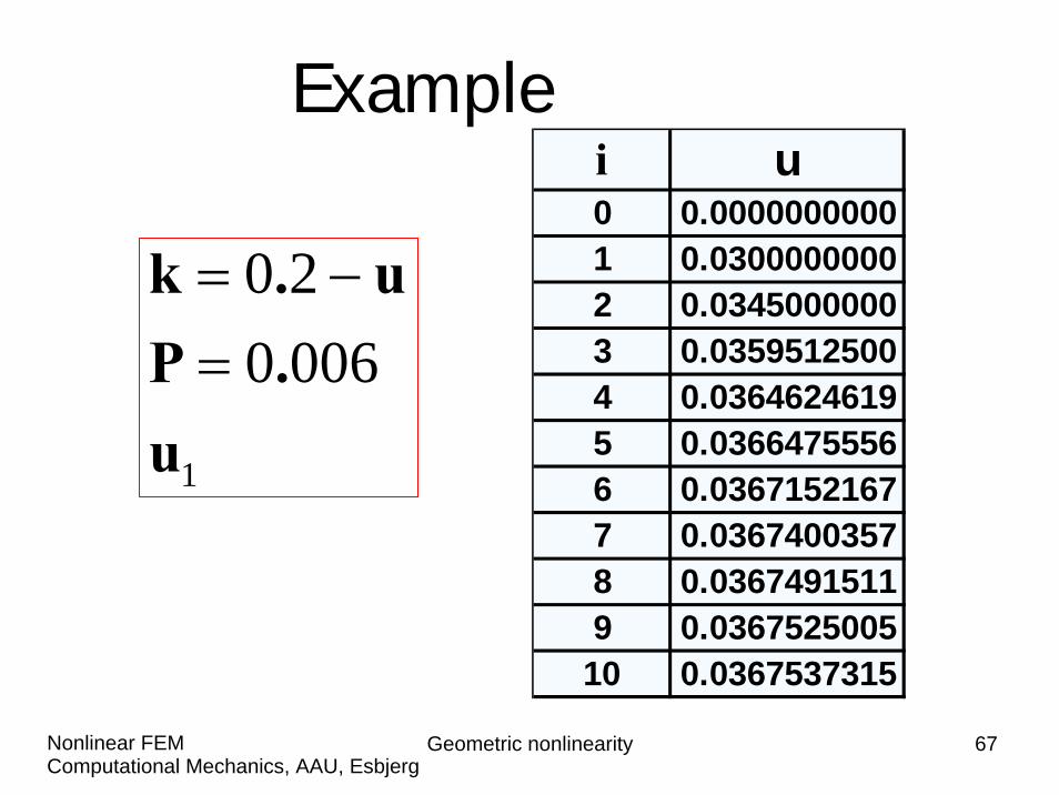
Example:P= 0.006
k u Del u0.2000000000 0.03000000000.1700000000 0.0352941176 15.00000000%0.1647058824 0.0364285714 3.11418685%0.1635714286 0.0366812227 0.68877551%0.1633187773 0.0367379679 0.15445930%0.1632620321 0.0367507370 0.03474506%0.1632492630 0.0367536116 0.00782121%0.1632463884 0.0367542587 0.00176085%0.1632457413 0.0367544045 0.00039645%0.1632455955 0.0367544373 0.00008926%0.1632455627 0.0367544447 0.00002010%0.1632455553 0.0367544463 0.00000452%0.1632455537 0.0367544467 0.00000102%0.1632455533 0.0367544468 0.00000023%0.1632455532 0.0367544468 0.00000005%

Geometric nonlinearity 62Computational Mechanics, AAU, EsbjergNonlinear FEM
Load - Deflection
0.000
0.003
0.005
0.008
0.010
0.013
0.015
0.018
0.020
0 0.01 0.02 0.03 0.04 0.05 0.06 0.07 0.08 0.09
u
P

Geometric nonlinearity 63Computational Mechanics, AAU, EsbjergNonlinear FEM
Direct Substitution Alternative
1. Let load PA be applied to a softening spring.2. Assume kN = 0 for the first iteration. 3. Compute first approximation to displacement:
u1 = PA/k0
4. Take nonlinear term to other RHS.5. Compute next approximation to displacement:
u2 = (PA-kN1u1)/k0
6. Generate sequence of approximations.

Geometric nonlinearity 64Computational Mechanics, AAU, EsbjergNonlinear FEM
( )( )
( )iNiA1
01i
22NA1
03
11NA1
02
A1
01
ukPku
ukPku
ukPku
Pku
−=
−=
−=
=
−+
−
−
−
Sequence of Operations

Geometric nonlinearity 65Computational Mechanics, AAU, EsbjergNonlinear FEM
u
P
PA
u1
k0
a
1P1

Geometric nonlinearity 66Computational Mechanics, AAU, EsbjergNonlinear FEM
u
P
PA
u1
k0
a
1P1
IkN1u1
2
b
Geometric nonlinearity 67Computational Mechanics, AAU, EsbjergNonlinear FEM
i u0 0.00000000001 0.03000000002 0.03450000003 0.03595125004 0.03646246195 0.03664755566 0.03671521677 0.03674003578 0.03674915119 0.0367525005
10 0.0367537315
1
006020
u.P
u.k=
−=
Example

Geometric nonlinearity 68Computational Mechanics, AAU, EsbjergNonlinear FEM
Comparison
1. First approach requires [K] to be formulated and reduced in each step.
2. Second approach requires 1 formulation and reduction of [K0]
3. Second approach usually has more iterative cycles than first approach.
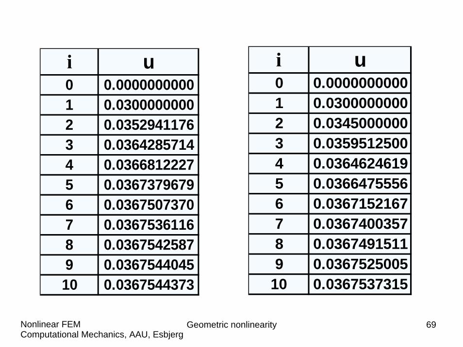
Geometric nonlinearity 69Computational Mechanics, AAU, EsbjergNonlinear FEM
i u0 0.00000000001 0.03000000002 0.03450000003 0.03595125004 0.03646246195 0.03664755566 0.03671521677 0.03674003578 0.03674915119 0.0367525005
10 0.0367537315
i u0 0.00000000001 0.03000000002 0.03529411763 0.03642857144 0.03668122275 0.03673796796 0.03675073707 0.03675361168 0.03675425879 0.036754404510 0.0367544373

Geometric nonlinearity 70Computational Mechanics, AAU, EsbjergNonlinear FEM
( )
( )10
111
1
1
<β<
β−+β=
−=Δ
Δβ+=
++
+
+
iii
iii
iii
uuuuuu
uuu
Under-Relaxation

Geometric nonlinearity 71Computational Mechanics, AAU, EsbjergNonlinear FEM
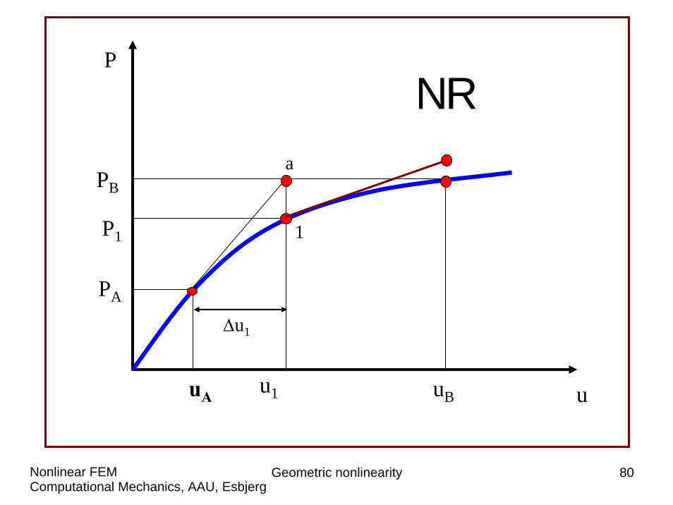
Newton-Raphson Approach
( )
11
0
ududP)u(f)uu(f
)u(fkPukk
AAA
ANA
AANA
Δ⎟⎠⎞⎜
⎝⎛+=Δ+
=
=+
:Series Taylor TermOne

Geometric nonlinearity 72Computational Mechanics, AAU, EsbjergNonlinear FEM
Newton-Raphson Approach
( ) ( )
t
NN
AAA
kdudP
duukdkukuk
dud
dudP
ududP)u(f)uu(f
=
+=+=
Δ⎟⎠⎞⎜
⎝⎛+=Δ+
Stiffness Tangent
00
11
kt - Tangent stiffness

Geometric nonlinearity 73Computational Mechanics, AAU, EsbjergNonlinear FEM
Newton-Raphson Approach
( )
( )( ) AB1tA
1tAAB
B1A
1
PPukukPP
Puuf
:thatsuchu:Seek
−=Δ
Δ+=
=Δ+
Δ
PB - PB - Load imbalance

Geometric nonlinearity 74Computational Mechanics, AAU, EsbjergNonlinear FEM
Newton-Raphson Approach
( )ii1i
iBiit
uuuPPuk
Δ+=
−=Δ
+
PB - Pi - Load imbalance

Geometric nonlinearity 75Computational Mechanics, AAU, EsbjergNonlinear FEM
u
P
PA
u1
P1
uA uB
PBa
1

Geometric nonlinearity 76Computational Mechanics, AAU, EsbjergNonlinear FEM
u
P
PA
u1
P1
uA uB
PBa
1
b
2
Δu1 Δu2

Geometric nonlinearity 77Computational Mechanics, AAU, EsbjergNonlinear FEM
uA uB kNA kt PA PB DEL u0.0000000000 0.0300000000 0.000000 0.200000 0.000000 0.0060 0.03000000000.0300000000 0.0364285714 -0.030000 0.140000 0.005100 0.0060 0.00642857140.0364285714 0.0367536116 -0.036429 0.127143 0.005959 0.0060 0.00032504010.0367536116 0.0367544468 -0.036754 0.126493 0.006000 0.0060 0.00000083520.0367544468 0.0367544468 -0.036754 0.126491 0.006000 0.0060 0.0000000000
Newton Raphson

Geometric nonlinearity 78Computational Mechanics, AAU, EsbjergNonlinear FEM
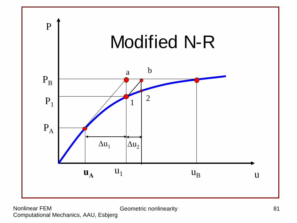
Modified Newton-RaphsonApproach
Do not update kt every iteration!

Geometric nonlinearity 79Computational Mechanics, AAU, EsbjergNonlinear FEM
Newton-Raphson Approach
( )( )
iii
iBit
uuu
PPukold
Δ+=
−=Δ
+1
PB - PB - Load imbalance
Geometric nonlinearity 80Computational Mechanics, AAU, EsbjergNonlinear FEM
u
P
PA
u1
P1
uA uB
PBa
1
Δu1
NR
Geometric nonlinearity 81Computational Mechanics, AAU, EsbjergNonlinear FEM
u
P
PA
u1
P1
uA uB
PBa
1
b
2
Δu1 Δu2
Modified N-R

Geometric nonlinearity 82Computational Mechanics, AAU, EsbjergNonlinear FEM
Comparison
1. Modified N-R has less calculations per iteration.
2. Modified N-R has more iterations.

Geometric nonlinearity 83Computational Mechanics, AAU, EsbjergNonlinear FEM
Incremental Approach
1. Apply loads in a number of small increments.
2. Iterate and Converge for each increment.3. Create entire load-displacement history.

Geometric nonlinearity 84Computational Mechanics, AAU, EsbjergNonlinear FEM
u
P
Purely incremental approach with no corrections.

Geometric nonlinearity 85Computational Mechanics, AAU, EsbjergNonlinear FEM
( )
ΔPdudPk
ufP
t
:increments Load
=
=
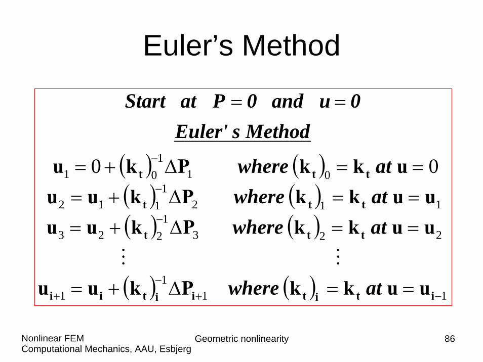
Euler’s Method
Geometric nonlinearity 86Computational Mechanics, AAU, EsbjergNonlinear FEM
( ) ( )( ) ( )( ) ( )
( ) ( ) 111
1
2231
223
1121
112
011
01 00
−+−
+
−
−
−
==Δ+=
==Δ+===Δ+===Δ+=
==
ititiitii
ttt
ttt
ttt
uukkPkuu
uukkPkuuuukkPkuu
ukkPku
at where
at where at where at where
Method sEuler'0u and0 P at Start
Euler’s Method

Geometric nonlinearity 87Computational Mechanics, AAU, EsbjergNonlinear FEM
( ) ( )[ ]
( ) gukkP
PP
PPPkuu
iNiR
i
iRiiitii
iSprinthe of Load Resisting
Load Applied Externally
+=
Δ=
−+Δ+=
∑+
−+
0
1
11
1
Incremental with Load Correction

Geometric nonlinearity 88Computational Mechanics, AAU, EsbjergNonlinear FEM
u
P
Incremental approach with Load Corrections.

![Vega: Nonlinear FEM Deformable Object Simulatorrun.usc.edu/vega/SinSchroederBarbic2012.pdf · Vega: Nonlinear FEM Deformable Object Simulator ... (CalculiX [DW]) deformable ... J.](https://static.fdocuments.in/doc/165x107/5aecb8f27f8b9a3b2e8f8865/vega-nonlinear-fem-deformable-object-nonlinear-fem-deformable-object-simulator.jpg)