Geometric Assessment Summary: Lidar, DEM and … Assessment Summary: Lidar, DEM and Satellite data...
20
Geometric Assessment Summary: Lidar, DEM and Satellite data U.S. Department of the Interior U.S. Geological Survey Ajit Sampath, SGT Contractor to USGS EROS JACIE 2016 | April 11-15, Ft. Worth, TX
Transcript of Geometric Assessment Summary: Lidar, DEM and … Assessment Summary: Lidar, DEM and Satellite data...

Geometric Assessment Summary: Lidar,
DEM and Satellite data
U.S. Department of the Interior
U.S. Geological Survey
Ajit Sampath, SGT Contractor to USGS EROSJACIE 2016 | April 11-15, Ft. Worth, TX

Outline
• Data Assessment
• Geiger and Sigma Space Lidar
• Vricon DEM
• RapidEye
• Deimos-2
• Geometric Assessment Methodologies
• Results
• Summary

Geiger Mode and Sigma Space Lidar
data
• Analysis of data only
• Sensor independent
• Perhaps some inferences on the processes
• Geometric Accuracy
• Accuracy of derived features and not so much
individual points
• Comparison with USGS Lidar data and
• Visual comparisons
• Surface variability analysis
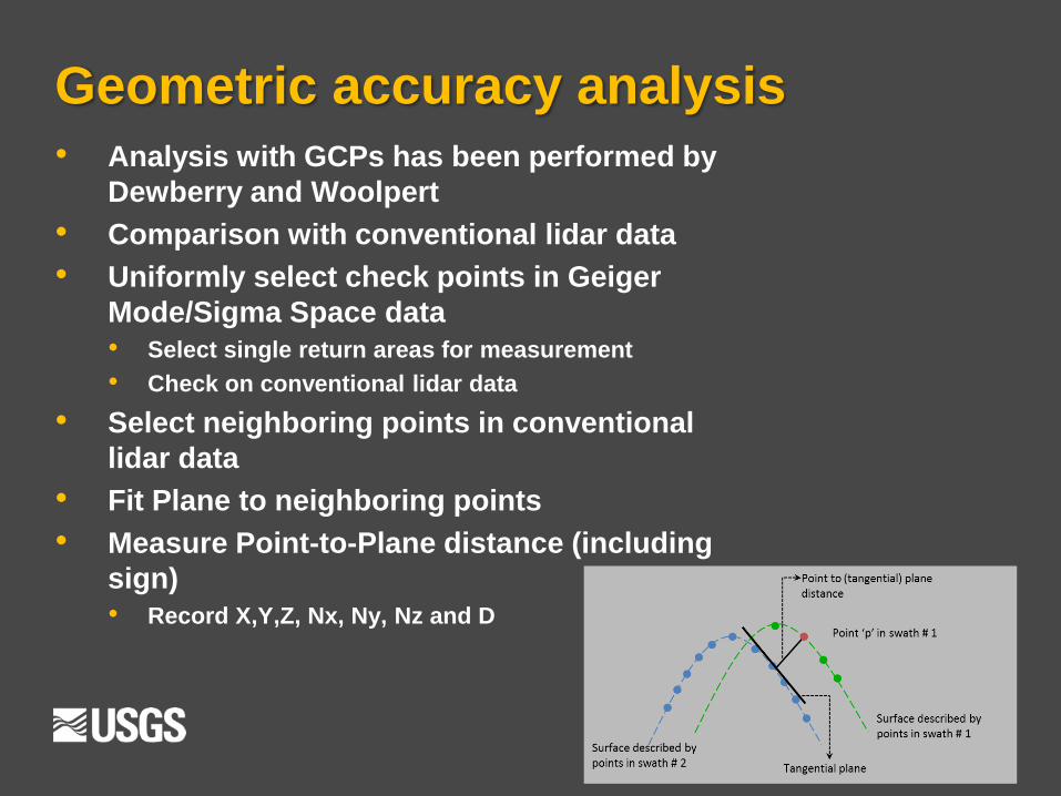
Geometric accuracy analysis
• Analysis with GCPs has been performed by
Dewberry and Woolpert
• Comparison with conventional lidar data
• Uniformly select check points in Geiger
Mode/Sigma Space data
• Select single return areas for measurement
• Check on conventional lidar data
• Select neighboring points in conventional
lidar data
• Fit Plane to neighboring points
• Measure Point-to-Plane distance (including
sign)
• Record X,Y,Z, Nx, Ny, Nz and D

Geometric Analysis
• Vertical Accuracy
• Use measurements flat areas:
Arc cosine of Nz < 5 degrees
• Compare the elevation values
i.e. D
• Horizontal Accuracy
• Identify measurements from
higher slopes
• Arc cosine of Nz > 10-15 degrees
• Use least squares solvers to
solve
• 𝑁Δ𝑋 = 𝐷 where N= [Nx Ny Nz]
• Obtain mean Δ𝑋 and standard
deviation

Geometric Analysis
• Geiger-Conventional Lidar
• dH: Mean -0.07 and RMSD 0.07
• Mean dX and dY: -0.11 and 0.18 respectively with low standard
deviation
• Sigma Space- Conventional
• dH: Mean -0.10 and RMSD 0.11
• Mean dX and dY: 0.15 and 0.05 respectively with low standard
deviation
• Quite possible that both Geiger and Sigma Space lidar data are
more accurate than conventional lidar data
• Ground based static lidar or perhaps mobile lidar data will be
better for such analysis

Sigma-Geiger USGS
Geiger-Conventional
Lidar
Sigma Space-
Conventional Lidar

Roof Edges
Geiger Lidar
Sigma Space
Lidar
Conventi
onal Lidar
Conventional
Lidar

Conventional Lidar DEM

Geiger Mode DEM

Sigma Space DEM

Variability analysis
• Analysis similar to PCA
• Select locations uniformly
• Gather points in neighborhood
• Generate covariance matrix and determine eigen
values𝝀𝟏, 𝝀𝟐, 𝝀𝟑 𝒘𝒉𝒆𝒓𝒆 𝝀𝟏>𝝀𝟐>𝝀𝟑• Calculate 𝝀𝟑 as measure of variability
Mean SD
Geiger Mode 9.40E-04 0.28
Sigma Space 5.01E-04 0.37
Conventional Lidar 0.0014 0.53

Vricon DEM Analysis
• Digital Surface Model over Palmer, Alaska
provided by Digital Globe
• Data in UTM and heights are ellipsoidal
• Generated from multi-image nominally 50 cm
resolution satellite imagery
• Reference Data
• Lidar data in state plane and elevation were
orthometric
• Reference data were converted to match Vricon
DSM

Vricon DEM Analysis
• Spot Heights over• Clear and open areas
• Sloping surfaces (building roof)
• Linear surfaces like roads
• Mean of -0.27 m and SD of 1.69 m
• Some points to ponder:
• Matches very well in clear and open areas (< 40 cm)
• Sloping areas have higher differences
• Discrepancy appears near trees etc.
• Probably due to satellite look angles
• Horizontal errors need to be checked further
• Appears to be within the 1.5 m of Lidar
• Lidar may not be horizontally accurate

Geometric Accuracy Assessment• Performed using the Landsat Image Assessment System (IAS)
• Developed for Radiometric and Geometric Characterization and Calibration for Landsat data.
• Band to Band (B2B) assessment• B2B is performed to test band alignment of the image data • It is typically done by registering each band against every other band
• Image to Image (I2I) registration assessment tool• I2I is usually performed to compare the relative accuracy between two images• Performed against an image of higher accuracy (reference data)• The results provide an insight to the relative accuracy of the search image
with respect to the reference image• When the correlated points are plotted in the image, it also helps to detect any
systematic bias in the image

Geometric Accuracy Assessment
• Assessed by comparing relative positional of two images
• The input consists of a reference image and a search image
• The reference image and the corresponding pixels in the study image inputs are
uniformly sampled (using the image geolocation/header information).
• Image chips (a window of 64 x 64 or 32 x 32 pixels) for reference and study images
are selected around these samples.
• Normalized cross-correlation values were generated between the center of the
reference image chip, and the pixels in the study image chip.
•
• CC(l,s) is the normalized cross correlation coefficient at location (l,s), and
refer to the intensities associated with reference and study image windows,
and refer to the mean intensities within the window.

RapidEye Overview
• Over 60 datasets Data from five-satellite RapidEye (RE) commercial EO
constellation were provided by Andreas Brunn
• Five spectral bands
• Blue, Green, Red, Near Infrared, Red-Edge
• Ground sampling distance: 6.5 m (nadir), Pixel size (orthorectified): 5 m
• Image Size: 25km X 25km
• Data for analysis in WGS UTM Zone 13N (Pueblo) and 14N (Sioux Falls) and
rail Road Valley
• Reference data: Orthoimagery

Rapid Eye Analysis
• Analysis of 45 data sets over Sioux Falls, Pueblo
and Rail Road Valley
• Band registration and absolute accuracy analysis
• Pueblo: 15 images
• Sioux Falls:35 images
• RVPN: Band registration checks only
• All bands registered to less than 0.1 pixels except
band 5, which was 0.15 pixels
Line Sample RMSE L RMSE S
Average -0.39 -0.59 0.50 0.64
StdDev 0.37 0.20 0.30 0.17
Range -1.23 -0.78 -0.91 -0.68
Line Sample RMSE L RMSE S
Average -0.65 0.34 0.68 0.49
StdDev 0.42 0.34 0.41 0.22
Range -1.79 -1.26 -1.72 -0.76

Deimos-2
• Three datasets from Urthecast
• DC, Alaska and Sioux Falls
• Sioux Falls data set analyzed for
accuracy
• Reference data: Orthoimagery and
Ground Control Points over Sioux Falls
only
• Over 60 Check points and GCPs used
for the analysis
Line Sample
Mean 0.79 0.81
Standard Deviation 1.83 1.08
RMSE 1.98 1.35
Line Sample
Mean 1.07 0.35
Standard Deviation 1.76 1.25
RMSE 2.05 1.29

Continuing Analysis
• Deimos-2
• MTF and Spatial Resolution analysis
• Planet Labs
• Geometric, Radiometric and Spatial Resolution
analysis
• Vricon DEM
• Further Analysis of “what to expect?”
• Spatial resolution tests
• More Collaboration!
• Please contact me at [email protected]
• Or Greg Stensaas at [email protected]