Geometric and Visual Reconstruction of Binary Shapes
121
University of Szeged Faculty of Science and Informatics PhD School in Computer Science Thesis Geometric and Visual Reconstruction of Binary Shapes Author: J´ ozsef N´ emeth Supervisors: J´ anos Csirik, DSc Zolt´ an Kat´ o, DSc A dissertation submitted for the degree of doctor of philosophy of the University of Szeged Szeged, 2015
Transcript of Geometric and Visual Reconstruction of Binary Shapes

University of Szeged
Faculty of Science and Informatics
PhD School in Computer Science
Thesis
Geometric and Visual Reconstruction of
Binary Shapes
Author:
Jozsef Nemeth
Supervisors:
Janos Csirik, DSc
Zoltan Kato, DSc
A dissertation submitted for the degree of doctor ofphilosophy of the University of Szeged
Szeged, 2015


Acknowledgements
First of all, I would like to thank Janos Csirik for his guidance and support and for
that he made it possible for me to carry out my doctoral studies, and Zoltan Kato who
introduced me to the wonderful world of scientific research. I am also very thankful to
Csaba Domokos for his invaluable help and for sharing his knowledge and experiences.
I am grateful to Peter Balazs, Laszlo Varga, Marton Balasko, Antal Nagy, Laszlo
Nyul, Attila Tanacs and Kalman Palagyi who gave me some good advice and also
often provided me program codes and data for my experiments. I also appreciate the
friendship and support of Erika Griechisch, Norbert Hantos, Gabor Nemeth, Andras
London and Tamas Nemeth.
Last but not least, I am thankful to my parents who always supported and encour-
aged my education, to my brother Adam and to my girlfriend Eszter for their love and
support.
My work was supported by the Doctoral School of the University of Szeged, Foun-
dation for Education and Research in Informatics.
i


Contents
1 Introduction 1
1.1 Binary Image Processing . . . . . . . . . . . . . . . . . . . . . . . . . 3
1.1.1 Discrete Tomographic Reconstruction . . . . . . . . . . . . . . 3
1.1.2 Binary Image Deconvolution . . . . . . . . . . . . . . . . . . . 4
1.1.3 Binary Shape Registration . . . . . . . . . . . . . . . . . . . . 5
1.2 Summary by Chapters . . . . . . . . . . . . . . . . . . . . . . . . . . 7
1.3 Summary of the Author’s Contributions . . . . . . . . . . . . . . . . . 8
2 Discrete Tomography with Unknown Intensity Levels 11
2.1 Basic Concepts and Notations . . . . . . . . . . . . . . . . . . . . . . 12
2.2 The Reconstruction Method . . . . . . . . . . . . . . . . . . . . . . . 13
2.2.1 Optimization . . . . . . . . . . . . . . . . . . . . . . . . . . . 15
2.2.2 Estimation of the Discretization Parameter . . . . . . . . . . . 19
2.3 Gray-Level Independence and Implementational Details . . . . . . . . . 21
2.4 Numerical Experiments . . . . . . . . . . . . . . . . . . . . . . . . . 24
2.4.1 Comparison to the PDM-DART Method . . . . . . . . . . . . 26
2.4.2 Limited Angular Range Experiments . . . . . . . . . . . . . . . 28
2.4.3 Comparison to a Convex Programming Approach . . . . . . . . 30
2.4.4 Experiments with Valid Directon Sets of Uniqueness . . . . . . 32
2.4.5 Real Data Experiments . . . . . . . . . . . . . . . . . . . . . 33
2.5 Discussion . . . . . . . . . . . . . . . . . . . . . . . . . . . . . . . . 35
2.5.1 Complexity . . . . . . . . . . . . . . . . . . . . . . . . . . . . 35
2.6 Summary . . . . . . . . . . . . . . . . . . . . . . . . . . . . . . . . . 36
2.7 Appendix: The Lipschitz-Continuity of the Discretization Term . . . . 36
3 Binary Shape Deconvolution Using Discrete Tomography 41
3.1 The Restoration Method . . . . . . . . . . . . . . . . . . . . . . . . . 41
3.1.1 Deconvolution of the Projections . . . . . . . . . . . . . . . . 43
3.1.2 Binary Tomographic Reconstruction . . . . . . . . . . . . . . . 44
3.2 Experiments and Comparison . . . . . . . . . . . . . . . . . . . . . . 47
3.2.1 Experiments on Real Out of Focus Images . . . . . . . . . . . 50
iii

3.3 Summary . . . . . . . . . . . . . . . . . . . . . . . . . . . . . . . . . 50
4 Nonlinear Registration of Binary Shapes 53
4.1 A Parametric Reconstruction Framework . . . . . . . . . . . . . . . . 53
4.1.1 Construction of the System of Equations . . . . . . . . . . . . 56
4.2 The Studied Deformation Models . . . . . . . . . . . . . . . . . . . . 57
4.2.1 Planar Homography . . . . . . . . . . . . . . . . . . . . . . . 57
4.2.2 The Taylor Series Expansion of Planar Homography . . . . . . 59
4.2.3 Polynomial Transformations . . . . . . . . . . . . . . . . . . . 60
4.2.4 Thin Plate Spline . . . . . . . . . . . . . . . . . . . . . . . . 61
4.3 Implementational Details . . . . . . . . . . . . . . . . . . . . . . . . . 62
4.3.1 Numerical Implementation . . . . . . . . . . . . . . . . . . . . 63
4.3.2 Solution and Complexity . . . . . . . . . . . . . . . . . . . . . 64
4.4 Experiments on Synthetic Images . . . . . . . . . . . . . . . . . . . . 65
4.4.1 Comparison of Different ω Functions . . . . . . . . . . . . . . 66
4.4.2 Comparative Tests . . . . . . . . . . . . . . . . . . . . . . . . 68
4.5 Experiments on Real Images . . . . . . . . . . . . . . . . . . . . . . . 73
4.5.1 Planar Homography . . . . . . . . . . . . . . . . . . . . . . . 73
4.5.2 Thin Plate Spline . . . . . . . . . . . . . . . . . . . . . . . . 77
4.5.3 An Industrial Application . . . . . . . . . . . . . . . . . . . . 78
4.6 Summary . . . . . . . . . . . . . . . . . . . . . . . . . . . . . . . . . 79
5 Affine Invariants Based Projective Registration of Binary Shapes 81
5.1 The Registration Method . . . . . . . . . . . . . . . . . . . . . . . . 81
5.1.1 Decomposition of the Transformation . . . . . . . . . . . . . . 82
5.1.2 Estimation of the Perspective Distortion . . . . . . . . . . . . 83
5.1.3 Estimation of the Affine Component . . . . . . . . . . . . . . 84
5.2 Implementational Issues . . . . . . . . . . . . . . . . . . . . . . . . . 85
5.3 Experiments . . . . . . . . . . . . . . . . . . . . . . . . . . . . . . . 86
5.4 Discussion . . . . . . . . . . . . . . . . . . . . . . . . . . . . . . . . 87
5.5 Summary . . . . . . . . . . . . . . . . . . . . . . . . . . . . . . . . . 88
Appendices 89
A Summary in English 91
B Summary in Hungarian 95
iv
List of Figures
2.1 The discretization model and typical geometry types . . . . . . . . . . 12
2.2 Demonstration of how the minimization of the discretization term en-
forces binary sets . . . . . . . . . . . . . . . . . . . . . . . . . . . . . 15
2.3 Demonstration of the convergence of the proposed method . . . . . . 16
2.4 Estimation of discretization parameter α . . . . . . . . . . . . . . . . 20
2.5 Four of the phantom images used to evaluate the performance of the
proposed method. . . . . . . . . . . . . . . . . . . . . . . . . . . . . 23
2.6 Example noiseless and noisy projections for different incident beam in-
tensities. . . . . . . . . . . . . . . . . . . . . . . . . . . . . . . . . . 24
2.7 Some reconstruction results of the PDM-DART method and the pro-
posed method . . . . . . . . . . . . . . . . . . . . . . . . . . . . . . 27
2.8 Limited angular range experiments . . . . . . . . . . . . . . . . . . . 29
2.9 Comparison to a convex programming approach . . . . . . . . . . . . 31
2.10 A further comparison to a convex programming approach . . . . . . . 32
2.11 Reconstruction of a gas pressure regulator . . . . . . . . . . . . . . . 33
2.12 Gas pressure regulator: 3D visualization of the reconstruction results. . 34
3.1 The degradation model and the basic idea of the proposed method . . 42
3.2 A typical L-curve and its curvature . . . . . . . . . . . . . . . . . . . 43
3.3 The evolution of the estimation of the projection vector during the
iteration. . . . . . . . . . . . . . . . . . . . . . . . . . . . . . . . . . 44
3.4 Associated network for a 3× 3 case . . . . . . . . . . . . . . . . . . . 46
3.5 Reconstruction results for different s ∈ S scale values. . . . . . . . . . 47
3.6 Example reconstruction results on synthetic images . . . . . . . . . . . 49
3.7 Results on letters extracted from out-of-focus document images. . . . . 50
4.1 The registration problem . . . . . . . . . . . . . . . . . . . . . . . . . 54
4.2 The effect of various ω functions . . . . . . . . . . . . . . . . . . . . 56
4.3 Example deformation fields . . . . . . . . . . . . . . . . . . . . . . . 57
4.4 Example perspective distortion . . . . . . . . . . . . . . . . . . . . . . 58
4.5 Projective transformations . . . . . . . . . . . . . . . . . . . . . . . . 59
4.6 Example polynomial transformation. . . . . . . . . . . . . . . . . . . . 60
v

4.7 Example thin plate spline transformation. . . . . . . . . . . . . . . . . 61
4.8 Coverage of transformed shapes during the minimization process . . . . 62
4.9 Plots of tested ωi function sets. . . . . . . . . . . . . . . . . . . . . 66
4.10 Planar homographies: Example images from the synthetic data set and
registration results . . . . . . . . . . . . . . . . . . . . . . . . . . . . 69
4.11 Polynomial transformations and Thin plate spline transformations: Ex-
ample images from the synthetic data set and registration result . . . . 70
4.12 Sample observations with various degradations for testing robustness. . 72
4.13 Registration results on traffic signs . . . . . . . . . . . . . . . . . . . 74
4.14 Registration results on hip prosthesis X-ray images . . . . . . . . . . . 75
4.15 Registration results on traffic signs . . . . . . . . . . . . . . . . . . . 76
4.16 Sample images from the MNIST dataset and registration results . . . . 77
4.17 Registration results of printed signs . . . . . . . . . . . . . . . . . . . 78
5.1 The registration process . . . . . . . . . . . . . . . . . . . . . . . . . 85
5.2 Example images from the synthetic data set and registration results . . 87
5.3 Registration results on traffic signs . . . . . . . . . . . . . . . . . . . 88
vi

List of Tables
1.1 Correspondence between the thesis points and the publications. . . . . 8
2.1 The rNMP measures (%) and runtime performances (sec.) provided by
the PDM-DART method and the proposed method . . . . . . . . . . . 25
2.2 The rNMP measures (%) and runtime performances (sec.) provided by
the PDM-DART method and the proposed method . . . . . . . . . . . 26
3.1 Test results and comparison on the synthetic dataset . . . . . . . . . . 48
4.1 Comparison of the tested ωi sets . . . . . . . . . . . . . . . . . . . 67
4.2 Planar homography: Comparative tests of the proposed method on the
synthetic dataset . . . . . . . . . . . . . . . . . . . . . . . . . . . . . 69
4.3 Polynomial transformations and Thin plate spline transformations: Reg-
istration results . . . . . . . . . . . . . . . . . . . . . . . . . . . . . . 71
4.4 Test of the robustness against segmentation errors . . . . . . . . . . . 73
4.5 Comparative results on the MNIST database . . . . . . . . . . . . . . 77
5.1 Test results on the synthetic dataset . . . . . . . . . . . . . . . . . . 86
A.1 Correspondence between the thesis points and the publications. . . . . 94
B.1 A tezispontok es a szerzo publikacioinak kapcsolata. . . . . . . . . . . 98
vii


List of Algorithms
1 The tomographic reconstruction method . . . . . . . . . . . . . . . . . 17
2 Minimization with backtracking line search . . . . . . . . . . . . . . . . 18
3 Deconvolution of a projection vector . . . . . . . . . . . . . . . . . . . 45
4 Shape restoration using discrete tomography . . . . . . . . . . . . . . . 47
5 Pseudo code of the nonlinear registration framework . . . . . . . . . . . 65
6 Pseudo code of the affine invariants based projective registration method 84
ix


Chapter 1
Introduction
Binary shapes play important role in the field of image processing, due to that
1. the images of many real world objects are basically binary shapes, e.g., text
characters, traffic signs, bones or implants on X-ray images, etc.,
2. in most of the image processing applications at some point of the processing
pipeline the images are binarized (i.e., segmented).
In many cases, the additional information that we are working with a binary valued
image limits the number of possible solutions (the search space) thus it can help to
obtain more accurate results. For example, the linear inverse problems like tomography
and deconvolution are sometimes under-determined, and have many possible solutions.
In many other cases, these problems are over-determined and inconsistent due the the
noisy input data. Knowing that we are seeking a binary image restricts the search
space, and as a result, helps to find the (most accurate) solution. For example in the
case of tomography, binary images can be usually reconstructed accurately only from
a few projections.
In many other cases, however, the lack of rich intensity information makes it difficult
to deal with these binary images. For example image registration techniques commonly
work with previously established point pairs and these correspondences are usually
obtained based on the intensity patterns around the points. Thus in the case of binary
images these methods can not provide appropriate point correspondences. On the
other hand, in such cases we do not need to deal with the intensity change between
the images. Therefore many techniques have been presented previously to register
binary images using statistics of the point coordinates of the shapes.
This work is a summary of the author’s research results in the visual reconstruction
and the geometric registration of binary shapes. Most of the presented results and
techniques are related to statistical moments. In the analysis of binary shapes, these
1

2 Chapter 1. Introduction
statistics have many advantages. They give an easy-to-compute, compact, and robust
representation of an image or a comparable measure of one property of the shape.
Invariant moments, for example, keep their value when the shape undergoes in some
kind of deformation, thus they can be considered as similarity measures and can be
used for shape description or matching. Moreover, they also provide an efficient tool
for binary image registration.
For example, in Chapter 2, we use a kurtosis-like fourth-order statistics to enforce
binary solutions in a discrete tomography reconstruction method. This discretization
term plays two roles in the algorithm. First, it gives a measure of the binarity of
the intermediate solutions. At the same time, it is used to drive the reconstruction
towards a binary one, by gradually minimizing it as a functional of the solution. This
can be done using simple gradient based optimization technique, since this functional
is continuously differentiable. The advantage of the method is that it does not require
the estimation of the two intensities of the images. Instead, it estimates the mid-level
of the intensities using the discretization term.
A binary image registration method is proposed in Chapter 4 which involves covari-
ant function sets. These functions are integrated over the foreground (object) regions,
that results in generalized shape moments of the shapes. More specifically, using power
functions we obtain the geometric shape moments. These functions are covariant with
respect to the transformation, i.e., their values vary with the transformation, thus each
function constraints the transformation parameters. These constraints are formularized
as a system of nonlinear equation, which is solved by standard nonlinear optimizer and
the solution gives the parameters of the aligning transformation.
In Chapter 5, different kind of statistics are used for projective registration of binary
images. In the first step, to estimate the perspective component of the transformation,
affine moment invariants (AMIs) are used. These shape statistics are invariant to
the affine transformations (translation, rotation, scaling and shearing), while generally
covariant to perspective distortions, thus they can be used to set up a system of
equation, and its solution gives the perspective parameters. In the second step, using
third-order geometric moments we obtain a system of third-order equations, and its
solution gives the parameters of the affine component of the transformation.
The problems addressed in this work involve different mathematical tools. In each
chapter we used notation systems that we found to be appropriate to discuss the
given topic in a simple and comprehensible way. Nevertheless, it resulted in somewhat
inconsistent notations between the parts. Therefore we build up the notation system
in each chapter as we introduce the basic concepts of the given topic.

1.1. Binary Image Processing 3
1.1 Binary Image Processing
While intensity levels or colors allow better representation of a real-world scene, in many
cases the silhouettes provide enough information e.g. to recognize or align the objects.
Moreover binary images are usually easier to store, process and analyse then grayscale
images, and therefore many algorithms have been developed to deal specifically with
binary images. In this section, we briefly introduce the topics that we address in this
work and overview the related literatures.
1.1.1 Discrete Tomographic Reconstruction
Tomography focuses on the reconstruction of images from a set of their projections
taken from different angles. The projections are usually taken by exposing the object
to some radiation and measuring the loss of the particles on its other side [28, 49, 48].
This way, the interior structure of the object can be examined. Tomography is of high
importance in different areas, e.g., in medicine, biology, while it also can be applied in
industry. The theory of the tomographic reconstruction has been heavily studied, and
there are many algorithms that can provide accurate results when a sufficiently high
amount of projection data is available. Filtered Back Projection [49], Simultaneous
Algebraic Reconstruction Technique (SART [3]) and Simultaneous Iterative Recon-
struction Technique (SIRT [102, 39]) are some of the most widely used methods.
In the case of discrete tomography [46, 47], it is assumed that the image contains
only a limited number of different intensity levels, i.e., the object consist of only a few
different materials. This additional information limits the number of possible solutions,
thus helps to obtain high quality reconstructions even from few projections. Discrete
tomography can also been considered as a combinatorial problem. The combinatorial
properties of binary sets was addressed in [88]. In his work, Ryser introduced an
efficient method for the reconstruction of binary images from vertical and horizontal
projections.
The reconstruction of binary images from vertical and horizontal projections can
be traced back to the network flow problem, which can be solved in polynomial time.
This efficient solvability can also be generalized to more projections [15, 9, 68]. These
methods iteratively update the solution in each iteration step using only two projec-
tions and the result of the previous iteration. Another network flow based approach
described in [37], Gesu et al. first generates a set of initial reconstructions from dif-
ferent projection pairs, then evolutional algorithm is used to find an optimal solution.
Discrete tomographic reconstruction problems are often under-determined due to
the low number of projections and inconsistent due to measurement errors [103]. How-
ever, there can be found exact solutions in the case of special classes of binary im-
4 Chapter 1. Introduction
ages [19, 26, 69]. Furthermore, the projection angle selection also affects the quality
of the reconstructions [107, 98]. In [106], different projection angle selection strate-
gies have been examined. Since the reconstruction of binary images from more than
two projections is proved to be NP-hard [36], the researchers examined approximation
approaches to optimize the objective functionals, e.g., evolutional algorithms [8, 6, 37]
and simulated annealing [71].
In [25], a heuristic for binary tomography, called Binary Steering has been pro-
posed. The basic idea is to gradually enforce binary solutions between the consecutive
steps of a continuous reconstruction algorithm. In [92], Schule et al. proposed a
less heuristic binary steering approach based on D.C. (difference of convex functions)
programming. The D.C. method can provide accurate reconstructions even from few
projections. The objective functional prescribes that the image should satisfy the pro-
jection data, but also enforces binary solutions at the same time. The reconstruction
is performed by a primal-dual sub-gradient algorithm, applied to the convex-concave
decomposition of the functional. The authors also extended their work to multi-valued
objects [93]. Another extension of this approach for multi-valued discrete tomography
has been proposed in [108] with a modified energy function and an appropriate opti-
mization strategy. Some further approaches can be found in [111] and [63]. In [12],
Batenburg et al. introduced the Discrete Algebraic Reconstruction Technique (DART).
The main advantage of this method is that it is not restricted to binary images. The
algorithm first segments the initial continuous reconstruction, then iteratively improves
the result by updating only the boundary pixels. Experiments showed that the algo-
rithm provides accurate solutions. The method has also been successfully applied on
three-dimensional data [13].
Most of the discrete tomography algorithms assume that the intensity values are
accurately known [12, 92, 63, 26, 19, 71, 87]. However, in practice, these gray-levels
are usually unknown and can not been estimated in a straightforward way. Even when
the attenuation coefficients (i.e., the densities of the materials) are known, the imaging
device still has to be calibrated, and these calibration parameters usually change over
time due to the usage of the equipment. The non-uniqueness of the binary images in
the case of absorbed projections was examined in [53].
1.1.2 Binary Image Deconvolution
Enhancement of degraded images is a crucial step in many applications. Such distor-
tions usually come in many forms such as motion blur, camera misfocus and noise.
Misfocus and motion blur can be described as the convolution of the image with a so
called blurring function (filters while noise usually follows a specific distribution as a

1.1. Binary Image Processing 5
good approximation.
Many techniques can be found in the literature for digital image enhancement
including simple methods and more sophisticated algorithms. Unsharp masking [91]
is one of the widely used algorithms to enhance image contrast. The basic idea of
this method can from photography in which it is used since the first half of the 20th
century to increase the sharpness of images. Its digital version is applied in many
image processing softwares. Inverse filtering (or deconvolution) of images is another
basic idea for recovering an image that is blurred by a known low-pass filter. It tries
approximately inverting the process that caused the image to be blurred. Researchers
have been studying deconvolution methods for several decades, and have approached
the problem from different directions.
Deconvolution is linear inverse problem and thus in the case of noisy images it
requires regularization. This can be handled using the Wiener filter [112] which can
be used when the point-spread-function (PSF, the filter which was used to blur the
image) and the signal-to-noise ratio (SNR) are known. Blind deconvolution [56] is a
technique for those cases when the PSF is unknown. In this method the PSF and the
images is updated in each iteration step, and thus its convergence depends on how
accurate is the initial estimation of the PSF.
The deconvolution of binary images like document images has been addressed
by several researchers (see [51], [55], [59] and [95]). In most of these algorithms, the
problem is traced back the to the solution of a system of equations which then solved by
some iterative optimization technique. Although these methods are intensely studied,
they are still time-consuming and require good parameter settings which makes the
applications of them difficult in practice. The size of the point spread function is
usually also limited.
1.1.3 Binary Shape Registration
In most of the image processing applications a key step is the registration of images,
i.e., the estimation of the transformation which aligns one image to the other (see [119]
for a good survey). The overlapped images can be then combined or compared. Most
of the techniques assume linear transformation (i.e.. rigid-body, similarity of affine)
between the shapes, however in many applications nonlinear deformations [118] (e.g.,
projective, polynomial, elastic) need to be considered. For example, the estimation of
the parameters of a projective transformation (also known as planar homography) be-
tween two views of the same planar object has a fundamental importance in computer
vision. Other typical application areas include visual inspection [109], object match-
ing [16] and medical image analysis [27]. Good surveys can be found in [119, 64].

6 Chapter 1. Introduction
Classical landmark based (or correspondence based) methods usually trace back the
problem into the solution of a system of linear equations set up using the coordinates
of point pairs [45]. These point pairs are usually established by matching the intensity
value patterns around the points[62]. On the other hand featureless methods estimate
the transformation parameters directly from image intensity values over corresponding
regions[65].
In many cases, however, the images do not contain sufficent variety of graylevel
values (e.g., images of traffic signs or letterings), or suffered from intensity value
distortions (e.g., X-ray images). Although there are some time consuming methods
to cope with brightness change across image pairs [50], these conditions make the
classical brightness-based methods unreliable. In [35], Francos et al. propose a method
for the estimation of a homeomorphism between graylevel images. They showed how
to transform the problem into the solution of a linear system of equations, however
they assumed that the intensity values differ only by a zero mean Gaussian noise.
When the segmentations are available it is reasonable to solve the registration prob-
lem using the binary versions of the images [96, 40]. Most of the current approaches
are restricted to affine transformations. For example Domokos et al. showed that it
is possible to trace back the affine matching problem to an exactly solvable polyno-
mial system of equations [30]. Affine moments and invariants can also been used to
recover linear transformation [100]. In [116] Yezzi et al. proposed a variational frame-
work that uses active contours to simultaneously segment and register features from
multiple images and applied it to medical image registration, where 2D and 3D rigid
body transformations are considered. A statistics-based technique is described in [97]
for the registration of edge-detected images, which includes a well-defined measure of
the statistical confidence associated with the solution. Edge pixel matching is used to
determine the ”best” translations. The statistical method called the McNemar test is
used to determine which candidate solutions are not significantly worst than the best
ones. This was of confidence regions of the registration parameters can be determined.
This method, however, is limited to solving for 2D translations only [97].
Most of the nonlinear registration techniques use point correspondences [40, 114,
16]. Although there are robust keypoint detectors like SIFT [62] or SURF [41], these
can not be used for binary registration due to the lack of rich intensity patterns.
Belongie et al. proposed a nonlinear shape matching algorithm in [16]. The method
first establish point correspondences between the binary shapes using a novel similarity
metric, called shape context, which consists in constructing a log-polar histogram of
surrounding edge pixels. Then it uses the generic thin plate spline model to align the
shapes. The main advantage of this approach is that it does not require intensity
information. In [40], Guo et al. introduced a method to estimate diffeomorphic

1.2. Summary by Chapters 7
distortions between shapes, where point correspondences between the boundary points
of the shapes are estimated using simulated annealing.
In [1], Bronsetin et al. proposed a similarity metric for non-rigid deformable shapes
and they extended it to partial similarity. It has been showed that their similarity metric
can be used to solve the correspondence problem. In [114], Worz et al. proposed a
novel approximation approach for landmark-based elastic registration using Gaussian
elastic body splines. Other methods use variational techniques [67]. In [42], Tagare et
al. proposed a non-rigid registration algorithm based on L2 norm and information-
theory.
1.2 Summary by Chapters
Chapter 2 addresses the problem of discrete tomography. In this field, it is commonly
assumed that the intensity values of the images (i.e., the attenuation coefficients of
the materials) are accurately known a priori. In practice, however, this information is
usually not available and hard to determine. The author proposes novel reconstruction
method for those cases, when the intensity values are unknown. Using higher order
statistics based discretization term, the solution automatically converges to binary sets.
Comparative tests showed, that the proposed method is more robust to the projection
noise as a state-of-the-art algorithm. The method has also been successfully applied
on real data.
In Chapter 3, a binary tomography based image deblurring method is introduced.
Tikhonov regularization based 1-dimensional deconvolution is proposed to restore the
horizontal and vertical projections. In this approach, the L-curve method is used to
determine the regularization parameter which provides the best trade-off between the
norm of the residual (data-fit term) and the norm of the solution (smoothness). To
reconstruct the shapes from the restored projections, a maximum-flow based binary
tomography method is applied. Comparative synthetic tests showed that the method
can provide reliable result even in the case of low signal-to-noise ratio images, thanks
to that the L-curve method can provide a good regularization parameter for any noise
level. Results on real out-of-focus images are also presented.
In Chapter 4, the nonlinear registration of binary images is addressed. A general
framework is proposed to estimate the parameters of a diffeomorphism that aligns
two binary shapes. The framework is applied to different widely-used transformation
classes. Comparisons to other state-of-the-art methods are conducted and its robust-
ness to different type of segmentation errors is examined. The algorithm has also been
successfully applied in different real-world applications.
Chapter 5 introduce a technique to estimate the parameters of a planar homog-

8 Chapter 1. Introduction
[73] [74] [76] [75] [32] [72]
I. •II. •III. • • •IV. •
Table 1.1: Correspondence between the thesis points and the publications.
raphy transformation between binary shapes. In this method the planar homography
is decomposed into the perspective distortion and the affine transformation and the
parameters of these two parts are estimated separately in two consecutive steps. Com-
parative synthetic tests and results on real images are also presented.
1.3 Summary of the Author’s Contributions
In the followings the list of the key points of the dissertation is given. Table 1.3 shows
the connection between the thesis points and the publications of the author. The
planar homography related results of the thesis point III. was also previously presented
in [77].
I.) The author proposes a novel higher order statistics based binary tomography
reconstruction method for those cases, when the intensities on the images are
unknown. He proposes an objective functional in which a discretization term
is applied to enforce binary solutions. He propose to minimize the objective
functional by a graduated non-convexity optimization approach, in which the
weight of the discretization term is increased during the optimization process to
gradually enforce binary solutions. The mid-level of the intensities is estimated
directly to the intermediate solutions in each iteration step. He proposes to
estimate the mid-level as the minimum of the discretization term. The author
examines the convergence properties of the method and shows that the behaviour
of the method is independent of the value of the intensities. The robustness of
the algorithm against different strengths of projection noise is also demonstrated.
The author compares his algorithm to state-of-the-art methods and shows that
his approach is a good alternative. He also successfully applies his algorithm to
real projection data.
II.) A binary tomography base method for the deconvolution of binary images is
introduced. The author proposes to deconvolve the projections of the blurred

1.3. Summary of the Author’s Contributions 9
images using a Tikhonov regularization based algorithm. The optimal regulariza-
tion parameter is found by the L-curve method. A maximum-flow based binary
tomography method is proposed to reconstruct the shapes from their deblurred
projections, . He shows in comparative tests that his method provides more re-
liable results then another widely-used method. He also presents results on real
out-of-focus images.
III.) The problem of nonlinear registration of binary images is addressed. A general
registration framework is applied to trace back the registration problem to a
system of nonlinear equations. The author applies the framework to different
nonlinear transformation classes such as planar homography, polynomial trans-
formations, and thin plate splines. He goes into the implementational details
and shows that the equations can be written in three alternative forms which
improves the registration results. In the case of planar homography, the author
shows that the performance of the algorithm can be improved if the framework
is applied to the Taylor series expansion of the transformation. The author pro-
poses different ω function sets to construct the system of equations and compares
them. He proposes to normalize the equations to guarantee equal contribution
to the objective functional. The author compares the method to other state-of-
the-art methods on synthetic datasets. He also examines the robustness of the
algorithm against different types of segmentation errors. The author shows that
the method can be applied in different real world applications.
IV.) The author proposes an affine moment invariants based algorithm to estimate
the parameters of a planar homography transformation between binary shapes.
He shows how to decompose the transformation into a perspective and an affine
component and estimate their parameters separately in two consecutive steps.
He shows how to estimate the projective parameters of the transformation using
affine moment invariants. In the second step, an affine registration method is
used to determine the remaining parameters of the transformation. The author
compares the method to the algorithm presented in the previous thesis point and
shows results obtained by the algorithm on real images.


Chapter 2
Discrete Tomography with Unknown
Intensity Levels
Batenburg et al. proposed a semi-automatic solution called Discrete Gray Level Selec-
tion (DGLS) method for the estimation of the gray-levels [10]. This algorithm can be
used as a preprocessing step before the discrete tomography reconstruction. An initial
continuous reconstruction is obtained, and an expert user is asked to select regions on
the image that can be expected to contain constant gray-levels. This information is
then used to estimate the gray-levels corresponding to the selected regions. In those
cases, however, when the topology of the object is complex and does not contain
sufficiently large homogeneous regions, this method can not be used.
An automatic method to estimate the segmentation parameters (gray-levels and
threshold values) for the DART method has been proposed in [105]. This approach
is based on the projection difference as a cost function. The main drawback of this
approach is that it requires full DART reconstruction in each iteration step, there-
fore it is computationally inefficient. In [104], the DART method has been extended
with a more advanced segmentation technique called Projection Distance Minimization
(PDM) [11]. While in the original DART method the segmentation parameters are
fixed, the PDM-DART method re-estimates these parameters in each iteration step by
minimizing the distance between the projections of the intermediate segmented image
and the projection data. The results are comparable to those, that can be obtained
with the original DART, when the segmentation parameters are accurately known a
priori.
In signal processing and image processing, entropy and high order statistics play
important role to regularize the solutions [113, 22]. For binary deconvolution such
measures are used to prescribe binary values for the solutions in [115] and [58]. In [51],
Kim et al. proposed a blind deconvolution method for binary images with unknown
11

12 Chapter 2. Discrete Tomography with Unknown Intensity Levels
(a) (b) (c)
Figure 2.1: The discretization model (a) and the illustration of the parallel beam
geometry (b) and the fan beam geometry (c).
intensity levels. The objective functional included a discretization term (a normalized
kurtosis statistics) which enforces binary solutions. The only parameter of this term is
the mid-level of the intensity levels which is estimated simultaneously with the solution
using a gradient based trust-region-reflective method.
In this chapter, we introduce a a binary tomography reconstruction method which
applies the same higher order statistics based discretization term described in [51].
In our method, the weight of this term is increased during the optimization process
to gradually enforce binary solutions which results in a graduated non-convexity opti-
mization scheme [17]. The discretization parameter (mid-level) is estimated directly
to each intermediate solution, as an alternating minimization step.
2.1 Basic Concepts and Notations
We introduce the basic concepts of the binary tomography reconstruction problem.
Let the intensity values of the background pixels and the foreground (object) pixels
denoted by c1 and c2 respectively. The digital image of size h × w is represented
by the column vector x ∈ c1, c2n, where n = hw is the total number of the pixels.
Suppose that projections have been taken from k different angles and let li the number
of measurements in the ith projection vector. All projection data are contained by the
column vector p ∈ Rm, where m =∑k
i=1 li is the total number of measurements. The
projection acquisition process, as usually is modeled by the system of linear equations
Wx = p, (2.1)
where the matrix W ∈ Rm×n describes the projection geometry, i.e., wij represents the
contribution of the image pixel xj to the projection value pi (see Fig. 2.1). The most

2.2. The Reconstruction Method 13
frequently used beam geometry types in tomography as well as in binary tomography
include parallel beam, fan beam, and cone beam.
Basically a reconstruction of x can be obtained by solving the system of linear equa-
tions Eq. (2.1). However, due to the low number of projections and the measurement
errors (noisy projection data), the system in Eq. (2.1) is usually under-determined and
inconsistent [103]. While the fact that the image that we are seeking is binary valued
theoretically limits the number of possible solutions, in a combinatorial point of view,
the accurate restoration of binary matrices is generally NP-hard, even when the inten-
sity levels are accurately known. Moreover, herein we assume that the intensity levels
c1 and c2 are unknown, which makes the reconstruction problem even more difficult.
2.2 The Reconstruction Method
The reconstruction is performed by the minimization of the following objective func-
tional:
E(x, α, µ) = F (x) + λS(x) + µD(x, α), (2.2)
in which we formulated three expected properties of the solution. First, the data fidelity
term represents that x should satisfy the projections:
F (x) =1
2‖Wx− p‖2
2. (2.3)
It expresses that the solution should have projections close to the input projection
data p in the least squares sense and it is commonly used in the field of discrete
tomography (e.g., in [92, 108]). As usually in the case of linear inverse problems,
minimizing Eq. (2.3) alone would lead to non-feasible solutions, due to noisy projection
data [103]. To regularize the solution, the objective functional contains a smoothness
prior term
S(x) =1
2‖Lx‖2
2, (2.4)
where L is the discrete Laplacian regularization matrix, i.e., Lx gives the same result as
the 2-dimensional convolution with the Laplacian filter. This term penalizes solutions
with high norm of second derivatives but allows the formation of edges. Setting λ high
enforces smooth regions even if the projections are noisy. Using only the data and the
smoothness terms, the functional F (x) + λS(x) is convex, and its minimum provides
a continuous solution.
Binary reconstruction is imposed by the discretization term
D(x, α) = n‖x− α1n‖4
4
(‖x− α1n‖22)2− 1, (2.5)

14 Chapter 2. Discrete Tomography with Unknown Intensity Levels
where α is the discretization parameter, 1n denotes the length-n column vector of ones,
and ‖x‖p = (∑n
i=1 xpi )
1/pis the general vector norm. This functional is minimized by
binary images, if α is the mid-level of the intensity values, i.e., there exists d for which
|xi − α| = d, for every i = 1, . . . n [22]. In such cases, it has a value of 0, while it
reaches its maximum value n− 1 if all the pixel intensities are equal to α except one
pixel. Thus it is bounded, and moreover, two times continuously differentiable except
at x = α1n. Therefore standard gradient based optimization techniques can minimize
it efficiently. The discretization term D(x, α) is closely related to the fourth order
standardized moment (or kurtosis), except that the fourth and second moments are
normalized using the mid-level α instead of the mean of the values.
Setting the weight µ of the discretization term large allows only binary solutions as
it suppresses the other components of the energy functional. The following theorem
states that for any ξ > 0 a sufficiently high value of µ can be chosen such that the
discretization level (i.e., the value of the discretization term) will be at most ξ at the
minimum point of the energy functional.
Theorem 1. For any ξ > 0, there exists µ(ξ) ∈ R, such that if µ ≥ µ(ξ) and
(x, α) = arg minx,α
E(x, α, µ), then D(x, α) ≤ ξ.
Proof. Let ξ > 0 be fixed and let y ∈ Rn and β ∈ R be arbitrary such that D(y, β) =
0. Choose µ(ξ) = (F (y) + λS(y))/ξ. If µ ≥ µ(ξ) and (x, α) = arg minx,α
E(x, α, µ),
then
µD(x, α) ≤ E(x, α, µ) ≤ E(y, β, µ) = F (y) + λS(y) = µ(ξ)ξ ≤ µξ (2.6)
and the statement follows.
The reconstruction problem for given ξ > 0 and µ ≥ µ(ξ) can be defined as the
following minimization problem:
(x, α) = arg minx,α
E(x, α, µ). (2.7)
In Section 2.2.1, we propose a graduated optimization scheme to minimize Eq. (2.7)
by iteratively increasing the discretization weight µ and re-estimating x and the mid-
level α in each iteration step. While convergence to the global minimum is not guaran-
teed, our experiments showed the efficiency of the method. Since Theorem 1 does not
provide a sharp (minimum) threshold µ(ξ), thus instead of increasing µ until it reaches
a specific µ ≥ µ(ξ), it is more reasonable to terminate the minimization process once
the value of the discretization term gets below ξ. In this case, the result will be a local
minimum of the energy functional corresponding to the value of µ at the moment of
the termination.

2.2. The Reconstruction Method 15
(a) Initial data, (b) 1 iteration, (c) 5 iterations,
Dα(x)=0.4501 Dα(x)=0.2831 Dα(x)=0.0960
(d) 10 iterations, (e) 15 iterations, (f) 25 iterations,
Dα(x)=0.0306 Dα(x)=0.0052 Dα(x)=0.0000
Figure 2.2: Demonstration of how the minimization of Dα(x) enforces binary sets. (a):
The initial data x ∈ Rn, n = 100 is created as a mixture of two normal distributions
(µ1 = 0, σ1 = 0.2, µ2 = 1, σ2 = 0.3). (b-f): The resulting vectors after different
number of gradient descent iterations with α = 0.5.
For the sake of simple notation we will refer to the discretization term and the
objective functional by Dα(x) and Eα,µ(x), in those cases, when the discretization
weight µ and the discretization parameter α are fixed. Furthermore, the notation
Epα,µ(x) will be used whenever we want to emphasize that the objective functional is
constructed using the projection vector p.
2.2.1 Optimization
The proposed optimization approach is based on the observation that while the dis-
cretization term is minimized by binary images, it does not have other local minimums
(w.r.t. x). Fig. 2.2 demonstrates how the minimization of the discretization term by
simple gradient descent steps
x′ = x−∇Dα(x), (2.8)
initiating with a non-binary vector converges to a binary set. The original binary image,
that we are seeking, minimizes the discretization term, if the discretization parameter
α is equal to (c1 + c2)/2. Obviously, the value of this mid-level is initially unknown.

16 Chapter 2. Discrete Tomography with Unknown Intensity Levels
i=0 i=75 i=98 i=119 i=174 i=224
µ=0 µ≈414.8 µ≈1.3×10³ µ≈3.7×10³ µ≈5.5×10⁴ µ≈6×10⁵
α = 0.4205 α = 0.5239 α = 0.4667 α = 0.4706 α = 0.4869 α = 0.4970
D(x, α) = 1.11 D(x, α) = 0.74 D(x, α) = 0.31 D(x, α) = 0.15 D(x, α) = 0.03 D(x, α) = 0.00
Figure 2.3: Demonstration of the convergence of the proposed method. The columns
show intermediate reconstructions of Fig. 2.5(b) from 5 projections after different
number of iterations. In the first row, 3-dimensional plots of the images are shown, in
which the estimated mid-levels α are indicated by horizontal planes. The second and
third rows show the images and their α-thresholded versions. Below the images the
corresponding discretization weight µ, the estimated mid-level α and the value of the
discretization term D(x, α) can be found.
In the case of a binary image deconvolution method it was proposed [51], to optimize
the value of the mid-level along with the solution and the point-spread-function in
the same gradient descent based optimization process. However, we found that in
the case of our method it is more efficient to estimate the mid-level directly to each
intermediate solution x based on the analysis of the discretization function. Therefore
we propose the following graduated optimization approach for solving the optimization
problem in Eq. (2.7). Starting from an initial reconstruction x which is obtained by
the minimization of the objective functional without the discretization term (i.e., with
µ = 0), in each iteration step
1. Estimate the mid-level α for the current solution x.
2. Increase the weight of the discretization term (µ).
3. Refine the reconstruction x by locally minimizing the objective functional using
the new parameters α and µ.

2.2. The Reconstruction Method 17
Algorithm 1: The tomographic reconstruction method
Input : The projection data p and the projection geometry matrix W.
Output: The reconstructed image x.
Minimize E0,0(x) with the gradient descent method in Algorithm 2 to find the
initial reconstruction x.
Estimate α (see Section 2.2.2) and choose a sufficiently small initial
discretization weight µ.
while Dα(x) > ξ doRe-estimate x by locally minimizing the objective functional Eα,µ(x) using
the gradient descent method in Algorithm 2 initiated with the previous
minimum x.
Estimate α for the current solution x.
Increase the discretization weight (we set µ← 1.05µ).
end
Return with x.
This process increasingly enforces binary solutions while iteratively re-estimates the
mid-level. Note that the method does not require the estimation of the intensity
values during this process neither the thresholding of the intermediate solutions. The
main steps of the method can be found in Algorithm 1, while the implementational
details are discussed in Section 2.3.
The proposed minimization strategy follows a graduated optimization scheme. In
the first step, without the discretization term (i.e., with µ = 0), the gradient based
minimization can easily find a global minimum of the objective functional. Then as
we slightly increase the weight of the discretization term µ and re-estimate the mid-
level α, it is expected, that the local minimization finds the new global optimum, and
as experimental results show, the proposed method converges to accurate solutions.
Fig. 2.3 demontrates the evolution of the intermediate solutions.
In each iteration step, the objective functional is minimized using the current dis-
cretization parameter α and discretization weight µ . For minimization we used gradient
descent method with backtracking line search[78], which guarantees convergence by
finding a gradient descent step size t that not increases the objective functional. Since
Eα,µ is continuous (except at x = α1n), such a decreasing step size always exists in
the negative gradient direction. The pseudo code of the minimization process can be

18 Chapter 2. Discrete Tomography with Unknown Intensity Levels
Algorithm 2: Minimization with backtracking line search
repeatLet the search direction be g = −∇Eα,µ(x)
Set t = h/K∗(∇C) and choose β, c ∈ (0, 1) (we set
h = 8, β = 0.5, c = 0.5).
while Eα,µ(x + tg) > Eα,µ(x)− ct‖g‖22 do
t← βt
end
x← x + tg
until ‖tg‖22 ≤ δσ2(x)
found in Algorithm 2, in which the gradient of the objective functional is computed as
∇Eα,µ(x) = ∇F (x) + λ∇S(x) + µ∇Dα(x),
∇F (x) = WT (Wx− p),
∇S(x) = LTLx, (2.9)
∇iDα(x) = 4n
((xi−α)3
(‖x−α1n‖22)2− (xi−α)‖x−α1n‖4
4
(‖x−α1n‖22)3
),
where ∇iDα(x) denotes the ith element of ∇Dα(x).
An appropriate initial step-length for the line search process can be found by con-
sidering the Lipschitz-continuity [110] of ∇Eα,µ. Let the Lipschitz-constant of an
arbitrary Lipschitz-continuous function f : Ω → Rn, Ω ⊆ Rn denoted by K(f). If f
is continuous on Ω, then
K(f) = supx∈Ω‖J(f)(x)‖, (2.10)
where J(f) denotes the Jacobian matrix of f .
Let C(x) = F (x) + λS(x) the convex component of Eα,µ(x). Since
J(∇C) = WTW + λLTL (2.11)
is a constant matrix, thus an upper bound estimation for K(∇C) = ‖J(∇C)‖ can be
given by
K∗(∇C) = ‖J(∇C)‖1, (2.12)
where ‖J(∇C)‖1 is equal to the maximum column sum of the positive semidefinite
J(∇C).
It can been shown [110], that choosing step-length t ≤ 1/K(∇Eα,µ), the
gradient descent step will not increase the function value. Since K(∇Eα,µ) ≤K(∇C) + µK(∇Dα), thus K(∇C) ≤ K(∇Eα,µ). Therefore we propose to choose
2.2. The Reconstruction Method 19
t = h/K∗(∇C) as an initial step-length guess in Algorithm 2, with h ≥ 1 for the sake
of a faster convergence (we set h = 8).
The discretization term is also Lipschitz-continuous on an appropriately defined
subset Λ ⊆ Rn, and in Section 2.7 we estimate an upper bound K∗(∇Dα) for its
Lipschitz-constant. Therefore, K∗(∇Eα,µ) = K∗(∇C) + µK∗(∇Dα) is an upper
bound for K(∇Eα,µ) and a step size t∗ = 1/K∗(∇Eα,µ) can be chosen directly (i.e.,
without the line search process) with which the gradient descent step will not increase
the objective functional. However, for fast convergence Λ should be restricted to the
set of the next possible solutions in the direction of −∇Eα,µ, and K∗(∇Dα) should
be estimated locally on that Λ before each descent step. In our experiments, this
estimation was more time consuming, thus we present our numerical results using the
simple line search approach. However in a parallel implementation this direct step-
length estimation could be a good alternative. Moreover the Lipschitz-continuity of
the gradient of the whole energy functional is an important property which indicates
that it can be efficiently minimized by standard optimization techniques.
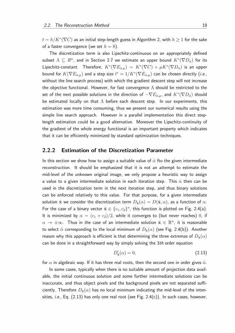
2.2.2 Estimation of the Discretization Parameter
In this section we show how to assign a suitable value of α fto the given intermediate
reconstruction. It should be emphasized that it is not an attempt to estimate the
mid-level of the unknown original image, we only propose a heuristic way to assign
a value to a given intermediate solution in each iteration step. This α then can be
used in the discretization term in the next iteration step, and thus binary solutions
can be enforced relatively to this value. For that purpose, for a given intermediate
solution x we consider the discretization term Dx(α) = D(x, α), as a function of α.
For the case of a binary vector x ∈ c1, c2n, this function is plotted on Fig. 2.4(a).
It is minimized by α = (c1 + c2)/2, while it converges to (but never reaches) 0, if
α → ±∞. Thus in the case of an intermediate solution x ∈ Rn, it is reasonable
to select α corresponding to the local minimum of Dx(α) (see Fig. 2.4(b)). Another
reason why this approach is efficient is that determining the three extremas of Dx(α)
can be done in a straightforward way by simply solving the 3th order equation
D′x(α) = 0, (2.13)
for α in algebraic way. If it has three real roots, then the second one in order gives α.
In some cases, typically when there is no suitable amount of projection data avail-
able, the initial continuous solution and some further intermediate solutions can be
inaccurate, and thus object pixels and the background pixels are not separated suffi-
ciently. Therefore Dx(α) has no local minimum indicating the mid-level of the inten-
sities, i.e., Eq. (2.13) has only one real root (see Fig. 2.4(c)). In such cases, however,
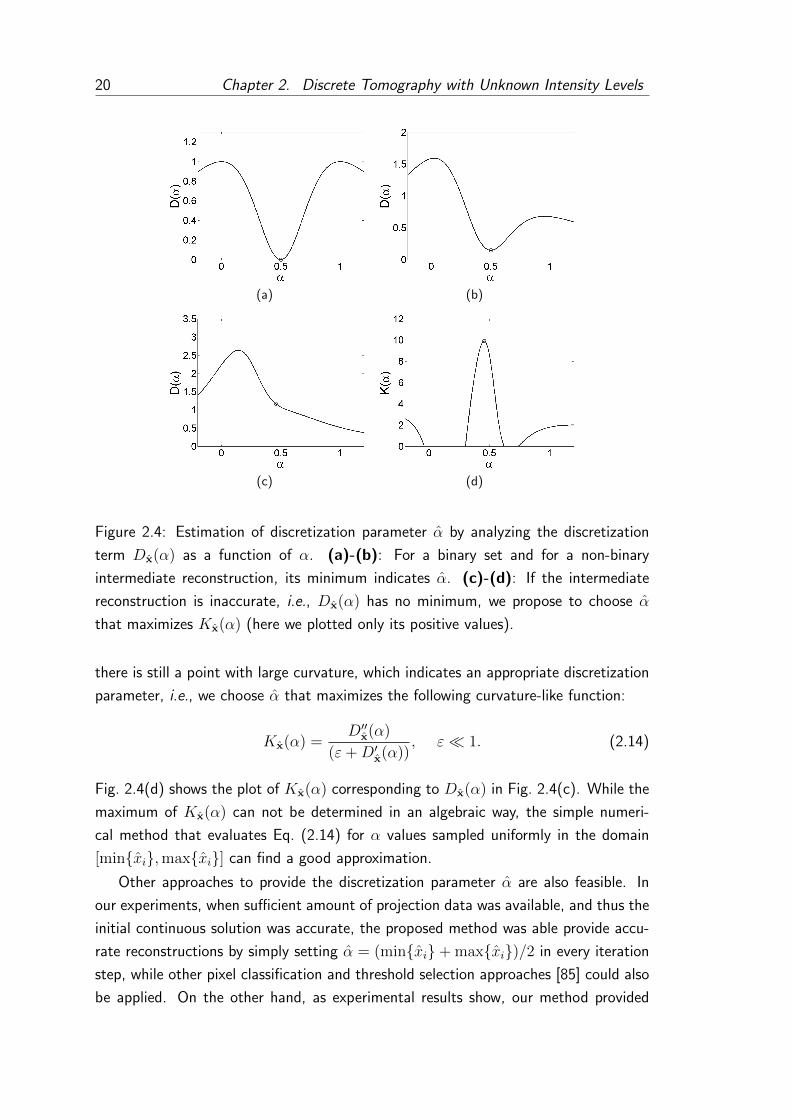
20 Chapter 2. Discrete Tomography with Unknown Intensity Levels
(a) (b)
(c) (d)
Figure 2.4: Estimation of discretization parameter α by analyzing the discretization
term Dx(α) as a function of α. (a)-(b): For a binary set and for a non-binary
intermediate reconstruction, its minimum indicates α. (c)-(d): If the intermediate
reconstruction is inaccurate, i.e., Dx(α) has no minimum, we propose to choose α
that maximizes Kx(α) (here we plotted only its positive values).
there is still a point with large curvature, which indicates an appropriate discretization
parameter, i.e., we choose α that maximizes the following curvature-like function:
Kx(α) =D′′x(α)
(ε+D′x(α)), ε 1. (2.14)
Fig. 2.4(d) shows the plot of Kx(α) corresponding to Dx(α) in Fig. 2.4(c). While the
maximum of Kx(α) can not be determined in an algebraic way, the simple numeri-
cal method that evaluates Eq. (2.14) for α values sampled uniformly in the domain
[minxi,maxxi] can find a good approximation.
Other approaches to provide the discretization parameter α are also feasible. In
our experiments, when sufficient amount of projection data was available, and thus the
initial continuous solution was accurate, the proposed method was able provide accu-
rate reconstructions by simply setting α = (minxi+ maxxi)/2 in every iteration
step, while other pixel classification and threshold selection approaches [85] could also
be applied. On the other hand, as experimental results show, our method provided
2.3. Gray-Level Independence and Implementational Details 21
accurate reconstructions even from low number of projections using the discretization
parameter estimation approach described in this section.
2.3 Gray-Level Independence and Implementational
Details
In this section, we discuss the implementational details and a practically important
property of the proposed method. In practice, the gray-levels can take values of differ-
ent orders of magnitude. It was a main purpose to develop our algorithm to provide
the same results, when it is applied to reconstruct images with different gray-levels
containing the same object. Without this property the algorithm would require to
set its certain parameters (e.g., the termination criterion thresholds and the initial
discretization weight), to the specific application.
Definition 1. The images x,y ∈ Rn are equivalent, if there exist u ∈ R and v ∈ R,
such that y = ux + v, where v = v1n.
For better understanding, it is worth pointing out that if x ∈ c1, c2n and y =
ux + v for some u, v ∈ R then y ∈ uc1 + v, uc2 + vn.
Definition 2. The projection data p ∈ Rm and q ∈ Rm are equivalent, if there exist
u ∈ R and v ∈ R, such that q = up + Wv, where v = v1n.
It can be easily seen that for a given projection matrix W , the projections of
equivalent images are also equivalent with the same u and v values. Moreover, the
binary images of the same object are equivalent.
By the gray-level independence of the proposed method we mean, that if it is
applied on two equivalent projection vectors, then the resulting reconstructed images
will also be equivalent. This property can be very useful in practice, because the
attenuation coefficients and thus the gray-levels can be highly variable. For example,
thanks to this independence, in our experiments on synthetic data and on real data,
the proposed method could be applied without any modification or fine-tuning the
termination criteria. Nevertheless, providing this property of the method is far from
trivial. The following statement ensures that applying gradient descent process on
equivalent intermediate solutions keeps their equivalence.
Theorem 2. Let the projection matrix W be fixed and let p and q equivalent pro-
jection vectors (in Def. 2.) for some u and v. Suppose that we apply the proposed
method on p and q simultaneously using the same regularization parameter λ, and at
certain points of the iteration processes

22 Chapter 2. Discrete Tomography with Unknown Intensity Levels
1. the intermediate solutions x and y are equivalent (in Def. 1.), and y = ux+v,
where v = v1n.
2. µ and τ are the discretization weights, and τ=u2µ.
3. α and β are the mid-level estimations, and β = uα + v.
After one gradient descent step in Algorithm 2, the resulting solutions x′ and y′ will
also be equivalent, and y′ = ux′ + v.
Proof. First consider the correlation of the two objective functionals:
Eq
β,τ(y) =
1
2‖W y − q‖2
2 +λ
2‖Ly‖2
2 + τDβ(y)
=1
2‖W (ux + v)− (up + Wv)‖2
2 +λ
2‖L(ux + v)‖2
2 + u2µDα(x)
=1
2‖u(W x− p)‖2
2 +λ
2‖u(Lx)‖2
2 + u2µDα(x) = u2Epα,µ(x), (2.15)
since Dβ(y) = Dα(x) and Lv = 0n. In a similar way, it can be shown that∇Eq
β,τ(y) =
u∇Epα,µ(x).
Let g1 = −∇Epα,µ(x) and g2 = −∇Eq
β,τ(y). Considering the termination criterion
of the line search method in Algorithm 2, it can be easily checked that:
Eq
β,τ(y + tg2) > Eq
β,τ(y)− ct‖g2‖2
2 ⇐⇒
⇐⇒ Epα,µ(x + tg1) > Ep
α,µ(x)− ct‖g1‖22, (2.16)
thus the line search method will terminate with the same step-length t, for both cases.
Performing one gradient descent step:
y′ = y + tg2 = ux + v + tug1 = u(x + tg1) + v = ux′ + v. (2.17)
In the followings, we discuss the implementation details of the algorithm. Using
these settings, one can easily check, that performing the algorithm on equivalent pro-
jection vectors, the conditions of Lemma 2 will always be fulfilled, independently of
what are the actual values of u and v. Therefore the method will perform gray-level in-
dependently, i.e., applying it on two equivalent projection vectors, the resulting images
will also be equivalent.

2.3. Gray-Level Independence and Implementational Details 23
(a) Phantom 1 (b) Phantom 2 (c) Phantom 3 (d) Phantom 4
Figure 2.5: Four of the phantom images used to evaluate the performance of the
proposed method.
Initialization: The first gradient descent minimization should be started from some
initial x. Since the energy functional without the discretization term is convex, the
initial point can be arbitrary. However, to provide gray-intensity independence we
choose the constant vector containing the average intensity value in each pixel:
xi =
∑mj=1 pj∑m
r=1
∑ni=1wri
. (2.18)
It can be easily checked, that the initial vectors calculated from equivalent projections
will be also equivalent.
Discretization weight: The graduated optimization scheme requires a small initial
discretization weight µ with which the discretization term does not suppress the other
components of the energy functional in the early iteration steps. Since the discretization
term is bounded, such µ can be selected based on the value of the energy functional
after the first minimization process. In our experiments µ = 10−2E0,0(x), where x is
the initial continuous reconstruction, provided a sufficiently small initial weight. From
Eq. (2.15) it follows that this choice fulfills the 2nd condition of Theorem 2.
Discretization parameter: If y = ux + v, then the method described in Sec-
tion 2.2.2 will provide α and β as the discretization parameters for x and y, such that
β = uα + v. This satisfies the 3rd condition of Lemma 2.
Gradient descent processes: To detect the convergence of the gradient descent
process in Algorithm 2, the step-length is compared to the normalized threshold δσ2(x).
We used δ = 2−25 in all of our experiments.
Termination criterion: As a termination criterion for the main loop of the algo-
rithm, the value of the discretization term is compared to ξ = 10−4, to detect if the

24 Chapter 2. Discrete Tomography with Unknown Intensity Levels
noiseless (I0 =∞) I0 = 105 I0 = 104
Figure 2.6: Example noiseless and noisy projections for different incident beam inten-
sities.
solution reached a sufficient discretization level. The value of the discretization term
is gray-level independent, i.e., if y = ux + v and β = uα + v, then Dα(x) = Dβ(y).
With these settings, performing the reconstruction algorithm on two equivalent
projections, the corresponding intermediate solutions and the final reconstructions will
also be equivalent. Implementing the algorithm this way helps to apply it on images
containing even highly different gray-levels, without any modification or parameter
refinement.
2.4 Numerical Experiments
To evaluate the performance of the proposed method, we used four phantom images
of size 256×256 (see Fig. 2.5). For these experiments we considered the parallel beam
projection geometry with equidistant line spacing. Different number of projections dis-
tributed equiangularly in the full angular range have been used. The distance between
the projection beams was 1 pixels in every direction. We performed our experiments
for both noiseless and noisy cases, where projection noise of two different levels has
been applied. In tomography, the projection data measured as the amount of parti-
cles reaching the detectors, and these particle counts are typically assumed to follow
Poisson distribution. The strength of the noise can be characterized by the incident
beam intensity (I0), which is the maximal number of particle count in the beams. This
noise model was recently used in [104], Here, we tested the methods for I0 = 105 and
I0 = 104, and the noiseless cases are referred by I0 =∞. As Fig. 2.6 shows, the first
amount provides somewhat weaker noise, while in the second case we get stronger dis-
tortions. The weight of the smoothness prior was set empirically to λ = 4.0, and this

2.4. Numerical Experiments 25
Phantom 1, I0 =∞PDM-DART Proposed
#p rNMP time rNMP time
4 0.79 9 1.07 48
5 0.43 13 0.66 51
8 0.09 9 0.07 37
12 0.01 20 0.02 33
Phantom 2, I0 =∞PDM-DART Proposed
#p rNMP time rNMP time
5 0.69 16 0.68 91
6 0.32 11 0.25 50
8 0.14 11 0.10 43
16 0.01 10 0.02 39
Phantom 1, I0 = 105
PDM-DART Proposed
#p rNMP time rNMP time
4 1.25 11 1.15 48
5 0.81 15 1.02 51
8 0.50 11 0.37 39
12 0.40 9 0.33 34
Phantom 2, I0 = 105
PDM-DART Proposed
#p rNMP time rNMP time
5 1.43 22 1.04 98
6 0.93 13 0.69 56
8 0.74 10 0.38 46
16 0.33 11 0.17 41
Phantom 1, I0 = 104
PDM-DART Proposed
#p rNMP time rNMP time
4 2.87 11 3.34 46
5 2.35 13 2.87 54
8 1.71 8 1.73 40
12 1.21 20 1.45 36
Phantom 2, I0 = 104
PDM-DART Proposed
#p rNMP time rNMP time
5 3.62 22 5.75 85
6 3.27 15 2.53 54
8 2.57 20 2.34 46
16 1.45 8 1.46 45
Table 2.1: The rNMP measures (%) and runtime performances (sec.) provided by
the PDM-DART method and the proposed method on Phantom 1 and Phantom 2
(Fig. 2.5) using different number of projections. The three rows show the results for
the three different strengths of noise applied on the projections. Bold values indicate
the better rNMP results for each test case.
value was used in all of these experiments. To evaluate the reconstruction results we
used the error measure called relative Number of Misclassified Pixels (rNMP), which
gives the ratio of the number of erroneous pixels and the number of object pixels in the
original phantom image. This error measure was recently used in [104] to evaluate the
results of the PDM-DART method. The rNMP measures and runtime performances
provided by the proposed method can be found in Table 2.1 and Table 2.2, while
Fig. 2.7 shows some reconstruction results.
26 Chapter 2. Discrete Tomography with Unknown Intensity Levels
Phantom 3, I0 =∞PDM-DART Proposed
#p rNMP time rNMP time
20 1.41 32 0.72 69
28 0.74 23 0.19 66
40 0.22 47 0.08 73
80 0.00 58 0.04 97
Phantom 4, I0 =∞PDM-DART Proposed
#p rNMP time rNMP time
28 10.46 41 9.68 88
36 7.03 66 6.23 96
40 5.89 86 4.99 98
80 2.16 64 1.78 127
Phantom 3, I0 = 105
PDM-DART Proposed
#p rNMP time rNMP time
20 2.09 25 1.39 71
28 1.21 23 0.57 65
40 0.90 48 0.25 73
80 0.08 53 0.05 99
Phantom 4, I0 = 105
PDM-DART Proposed
#p rNMP time rNMP time
28 11.82 63 10.10 86
36 8.51 55 7.05 102
40 7.16 50 5.60 98
80 2.74 113 1.98 126
Phantom 3, I0 = 104
PDM-DART Proposed
#p rNMP time rNMP time
20 5.61 21 4.67 75
28 4.41 30 3.83 71
40 3.52 24 2.94 82
80 1.91 76 2.01 123
Phantom 4, I0 = 104
PDM-DART Proposed
#p rNMP time rNMP time
28 16.30 60 13.53 86
36 12.70 91 11.00 97
40 12.48 103 10.00 101
80 8.58 60 5.37 146
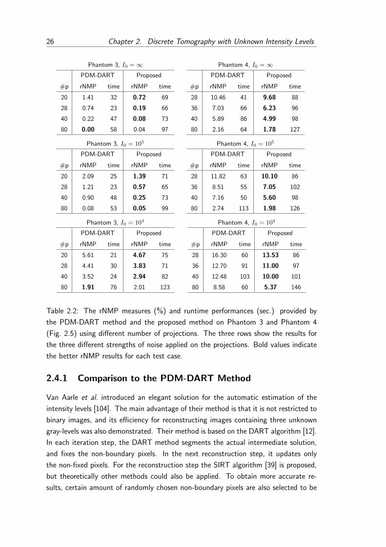
Table 2.2: The rNMP measures (%) and runtime performances (sec.) provided by
the PDM-DART method and the proposed method on Phantom 3 and Phantom 4
(Fig. 2.5) using different number of projections. The three rows show the results for
the three different strengths of noise applied on the projections. Bold values indicate
the better rNMP results for each test case.
2.4.1 Comparison to the PDM-DART Method
Van Aarle et al. introduced an elegant solution for the automatic estimation of the
intensity levels [104]. The main advantage of their method is that it is not restricted to
binary images, and its efficiency for reconstructing images containing three unknown
gray-levels was also demonstrated. Their method is based on the DART algorithm [12].
In each iteration step, the DART method segments the actual intermediate solution,
and fixes the non-boundary pixels. In the next reconstruction step, it updates only
the non-fixed pixels. For the reconstruction step the SIRT algorithm [39] is proposed,
but theoretically other methods could also be applied. To obtain more accurate re-
sults, certain amount of randomly chosen non-boundary pixels are also selected to be

2.4. Numerical Experiments 27
I0 = 105 I0 = 104
PDM-DART Proposed PDM-DART Proposed
Pha
ntom
1,4
proj
s.P
hant
om2,
4pr
ojs.
Pha
ntom
3,28
proj
s.P
hant
om4,
80pr
ojs.
Figure 2.7: Some reconstruction results of the PDM-DART method and the proposed
method. The misclassified pixels are depicted with dark.
non-fixed. This allows the formation of new boundaries that are not connected to the
boundary of the current solution. The noise of the projections and the errors caused
by the incorrectly fixed pixels can result in fluctuations in the updated values of the
non-fixed pixels. To overcome this issue, a Gaussian filter is applied to the intermedi-
ate solutions. While in the original description of the DART method this smoothing
operation was performed only on the non-fixed pixels, in the more recent work of the
authors [104] it was proposed to apply it on the whole image. We also found in our ex-
periments that this latter approach provides more accurate results. For the estimation
of the segmentation parameters, the projection distance minimization (PDM) method
has been proposed. The gray-levels and the threshold values are selected to obtain a
segmented image that satisfies the projection data the most.

28 Chapter 2. Discrete Tomography with Unknown Intensity Levels
For our tests, we basically set the parameters of the PDM-DART method according
to the author’s recommendations. As it was proposed, for termination criterion the
total projection error (TPE) was considered and the DART iterations was stopped if
TPE had not been decreased in the last 30 iterations. We selected randomly 1% of
the non-boundary pixels to remain non-fixed in each step. As it was recommended,
to reduce the additional computational cost introduced by the PDM method, the seg-
mentation parameter estimation was performed only once in every 10 iterations. Using
these settings in our experiments, the PDM-DART method was able to find the cor-
rect segmentation parameters and to converge to the right boundaries of the objects.
Nevertheless, we found that the choice of the radius of the Gaussian smoothing filter
strongly affects the results as follows. Applying weaker smoothing allows the PDM-
DART to converge to the right boundaries of the objects, and thus it provides accurate
reconstructions. At the same time, in the presence of stronger projection noise, the
large pixel-value fluctuations can only be handled by applying stronger smoothing,
which however blurs the important details in the case of complex shapes. The in-
fluence of the choice of the smoothing kernel on the reconstruction quality has been
recently investigated in [70]. In our experiments, the PDM-DART method was not
able to provide reliable results with the same smoothing kernel in each test case. Since
the adaptive selection of the kernel might be feasible, thus in order to make a fair com-
parison, we performed the PDM-DART method using smoothing kernels with different
deviations (σ = 0.5, 1.0, . . . , 3.0), and in each test case we chose the best result. As it
can be seen in Table 2.1 and Table 2.2, the proposed method is still more robust to the
projection noise, as it has been performed with the same weight of the regularization
term.
Both algorithms were implemented in Matlab R2008b and the experiments were
performed on an Intel Core2 Quad 2.66GHz CPU. As the results show in Table 2.1
and Table 2.2, PDM-DART required less computational time especially on the less
complex Phantom 1 and Phantom 2. This is due to that it updates only a relatively
small subset of the pixels in each step, while the proposed method updates all pixels
of the image. However, an efficient GPU based implementation, in which the update
steps could be performed on every pixel in a parallel way, could equalize the runtime
differences.
2.4.2 Limited Angular Range Experiments
In many applications, it is not possible to collect projection data from the full an-
gular range due to the size or the shape of the investigated object or the design of
the imaging device. To examine the performance of the methods in such scenarios,

2.4. Numerical Experiments 29
Figure 2.8: Limited angular range experiments. The rNMP measures as functions of
the angular ranges are plotted.

30 Chapter 2. Discrete Tomography with Unknown Intensity Levels
we generated 180 projections in the full angular range, corresponding to the angles
0, 1, 2, . . . , 179. We performed reconstructions using the projections in the inter-
vals of [0, φ] for φ = 4, 9, 14, . . . , 179, i.e., the number of projections increased
with the angular range. In Fig. 2.8, the rNMP errors are plotted against the angular
ranges. Since we obtained similar results for I0 = ∞ and I0 = 105, thus only the
results for I0 = 105 and I0 = 104 are presented. The PDM-DART method was able
to provide almost perfect reconstructions of Phantom 1 and Phantom 2, even from as
small range as [0, 49]. This is due to the efficiency of the DART method to converge
to the right boundaries of the objects, even in those cases, where the methods based on
the minimization of objective functionals (like the proposed algorithm) stuck in local
minima. However, on the more complex Phantom 3 and Phantom 4, the proposed
method provided more accurate results.
2.4.3 Comparison to a Convex Programming Approach
In [23], Capricelli and Combettes introduced a convex programming based approach for
noisy discrete tomography. The method traces back the problem to the minimization
of a convex function on the intersection of some appropriately constructed convex
sets. The advantage of this approach is that these sets can represent a wide range of
prior information (projection data, noise level estimation, binarity constraints, support
image, etc.). The minimized objective function was the square of the `2-norm of the
image in their experiments. The binarity promoting constraint prescribed upper bound
for the `1-norm (total variation) of the image. In their experiments the projections
was multiplied by 256 and Poisson noise was applied directly on the projection values.
The implementation of the method is available online [24] as a part of a convex
programming toolkit with an easy to use GUI . For discrete tomography the program
allows only 2, 3 or 4 equiangular projections, the measurements are given as the discrete
pixels sums along the four directions (horizontal, vertical and two diagonal pixel sums,
that consist of 256 − 256 and 511 − 511 measurements in the case of a 256 × 256
image). Therefore, we tested their algorithm on Fig. 2.5(a) using 4 projections. The
application provides an option to set the a priori values according to [23]. We tested
different combinations of a priori informations and settings, and we obtained the most
accurate result by using the a priori informations `1-norm, `2-norm, and the pixel range
together and the default algorithm settings. The method basically provides a ”close to
binary” solution but the segmentation of the results is also implemented. Fig. 2.9(a)
and Fig. 2.9(b) shows the output of the application and its binarization, the rNMP
error was 3.94%. We applied the proposed method on the same projection data using
the same projection geometry, and we obtained a 1.10% rNMP error (see Fig. 2.9(c)).

2.4. Numerical Experiments 31
(a) (b) (c)
Figure 2.9: (a): The reconstruction result obtained by the convex programming
method in [23] using four projections and (b): its discretization (rNMP=3.94%).
(c): The result obtained by the proposed method (rNMP=1.10%) using the same
projection data and projection geometry.
For a further comparison, we considered one of the numerical simulations described
in [23]. In this experiment, 4 projections were used to reconstruct the 32× 32 image
in Fig. 2.10(a). The histogram of the number of erroneous pixels on 2000 different
realization of the projection noise showed that their method misclassified about an
average of 8 pixels. Unfortunately the applied projection geometry is not clarified
in [23] for this experiment. Thus we conducted two tests using our method assuming
two different projection geometries:
1. In the first case, we considered parallel beam geometry with equidistant beam
spacing. The horizontal and vertical projections consisted of 32 − 32 measure-
ments, while the diagonal projections consisted of 45− 45 values.
2. In the second case, we applied the discrete pixel sums that is used by their online
available implementation. Here the horizontal and vertical projections consisted
of 32− 32, while the diagonal projections consisted of 63− 63 measurements.
For both cases we conducted a similar test on Fig. 2.10(a) using the proposed
method with λ = 0.1. 2000 realization of the projection noise was generated in
the same way as described in [23]. The histograms of the results can be found in
Fig. 2.10(b) and Fig. 2.10(c). It can be seen that for the equidistant beam spacing
geometry the proposed method produced less then 4 wrong pixels in more then 80%
of the test cases, while using discrete pixel sums it obtained perfect reconstruction in
almost all cases. Although this comparison was not performed on the same data as
in [23], the results are comparable due to the large number of randomly generated test
cases.

32 Chapter 2. Discrete Tomography with Unknown Intensity Levels
(a) (b) equidistant beam spacing (c) discrete pixel sums
Figure 2.10: (a): The test image used in [23]. (b)-(c): The results obtained by our
method on 2000 realization of the Poisson noise using 4 projections of the image on
the left with the two types of projection geometries. The histogram of the number of
missclassified pixels is plotted.
2.4.4 Experiments with Valid Directon Sets of Uniqueness
In [43], Hajdu addressed the problem of uniqueness in discrete tomography. It was
shown that for any image size h × w there exists a valid (i.e., non-trivial) set of four
lattice directions, such that any two objects can be distinguished by means of their
projections taken in those directions. In [20], it was shown that in fact whole families
of such suitable sets of four directions can be found.
Let (a, b) be a lattice direction with a, b ∈ Z and a, b coprime. The projection
value along a line parallel to (a, b) is computed as the sum of the intensities of those
pixels (grid points) that fall on the given line. This kind of projection model can play
an important role in the reconstruction of crystalline structures [14, 52].
In the first experiment, we considered 32 × 32 images and the direction set
(1, 3), (4, 5), (9, 7), (14, 15) which is valid for this size. This direction set provides
a relatively large amount of projection information. It results in a total number of
1560 projection lines and an average of only ≈ 2.63 pixels contribute to each pro-
jection value. In the second case, we considered 255 × 255 images and the direction
set (1, 0), (0, 1), (126, 127), (127, 126) with 97536 projection lines and an average
of only ≈ 2.66 pixels per projection value. Although theoretically these direction sets
ensure the uniqueness of the reconstructions, it is not guaranteed that a heuristic al-
gebraic reconstruction technique like the proposed method is able to find the exact
solutions in all cases. Indeed, the problem of finding the exact reconstruction from
four projections is generally NP-hard [36].
The aim of this experiment was to examine how often the proposed method is
able to find the exact solution. Due to the high amount of perfect (i.e., noiseless)
projection information regularization was not required, thus the algorithm was applied

2.4. Numerical Experiments 33
Figure 2.11: First colum: Four of the 18 projections of the homogeneous part of a
gas pressure regulator. Other columns: Reconstruction results of the PDM-DART
method (first row) and the proposed method (second row). The slices are indicated
on the first projection image.
with λ = 0. The proposed method was able to find the exact solutions on all of
the 32 × 32 and the 255 × 255 versions of our phantom images (Fig. 2.5). For
a further experiment, we generated 100 random binary images of size 255 × 255.
Each pixel of the images were set to 0 or 1 with probability 50%. The proposed
method reconstructed 88 images perfectly, while misclassified 4-4 pixels on 12 images.
We tested the PDM-DART method as well, which was also able to find the exact
solutions on the phantom images, while perfectly reconstructed 87 random images and
misclassified a total of 34 pixels. These results show that these methods are able to
converge to the exact reconstructions in most cases when the images are uniquely
determined by their projections.
2.4.5 Real Data Experiments
In [5], Balasko et al. compared the radiography and tomography possibilities of FRM-
II and Budapest Research Reactor. Classical Filtered Back Projection reconstruction
algorithm as well as discrete tomography methods have been tested. One of the exper-
iments has been presented on a gas pressure regulator of which upper part contained
only one material, thus binary tomography was possible. The reconstructions of the
horizontal slices of the gas pressure regulator were performed using 18 projections dis-
tributed on the half circle. These neutron radiography pictures were acquired in the
Radiography Station of the Budapest Research Reactor. The properties of the imag-
ing system are presented in [5] and [4]. The slices of the gas pressure regulator were
reconstructed separately, and fan beam geometry was assumed on each slice. Due
to the distorting properties of the image acquiring systems, some preprocessing steps
(e.g., intensity and uniformity corrections) were performed to prepare the projection

34 Chapter 2. Discrete Tomography with Unknown Intensity Levels
Figure 2.12: Gas pressure regulator. 3D visualization of the reconstruction results of
the PDM-DART method (1st row) and the proposed method (2nd row). In the first
column, half of the object is removed to show its inner structure.
data for reconstruction. Rigid-body registration algorithm was applied to correct image
plate misplacements. To reduce complexity, the projections were cropped and the rele-
vant parts were re-sampled. For discrete tomography, simulated annealing was chosen
to minimize the energy function. One of the main difficulties was that the attenua-
tion coefficients were unknown. These parameters were determined experimentally, by
performing reconstructions assuming different intensity levels.
We tested both the PDM-DART algorithm and the proposed method using 18
preprocessed projections of the gas pressure regulator provided by the authors of [5].
Four of the projections and some reconstruction results can be seen in Fig. 2.11. Each
line of the projections contained 309 measurements and the slices were reconstructed
on an image grid of size 309×309. A total of 88 horizontal slices of the homogeneous
part of the gas pressure regulator has been reconstructed. To visualize the separately
reconstructed slices altogether, 3D models has been created using marching cubes
algorithm, see Fig. 2.12. Similarly to the synthetic phantom experiments, the main
difficulty with the PDM-DART was to select the strength of the smoothing filter, that
provides smooth results but preserves the small details of the images at the same time,
2.5. Discussion 35
while the proposed method could be applied using the same parameter settings as in
the synthetic tests.
2.5 Discussion
In the previous sections, we examined the performance of the PDM-DART method
and the proposed method, and while both of the methods provided reliable results,
the proposed method is found to be more robust to the projection noise. The two
approaches are very different, and both methods have their advantages and drawbacks.
The main advantage of the PDM-DART method is that it can be applied to multi-level
images, while the proposed method has been developed to binary cases. In PDM-DART
there are some parameters (e.g., the width of the boundaries on which the update steps
are performed, the amount of randomly chosen non-fixed pixels, the strength of the
smoothing operations applied in each iteration steps) that affects the accuracy of the
reconstructions. These parameters have to be fine-tuned, and in our experiments we
had to perform the PDM-DART with different smoothing kernels in each test case to
find the settings that provides the best reconstruction. In contrary, the only parameter
of the proposed method that could affect its results is the weight of the smoothing
term, however, our method was able to provide competitive results using its same
setting in all test cases, which shows, that the proposed method less sensitive to the
strength of the projection noise.
In our experiments the proposed method provided reliable results using the smooth-
ness prior S(x) in both the weak and the strong noise cases. However, we did not
focus on the choice of S(x), which could be the subject of a future work. Theoret-
ically other regularization terms can also be applied directly in the proposed energy
functional. Also, the weight of the regularization can be chosen based on a priori in-
formation on the noise, while there are automatic regularization parameter estimation
techniques [7].
2.5.1 Complexity
In the case of two-dimensional images, the algorithm stores the O(m√n) non-zero
entries of the sparse matrix W , since each projection measurement is computed using
O(√n) pixels. For the sparse matrix L and the current solution x the method requires
O(n) space, while the gradient of the energy function needs O(m) space. Computing
the gradient and evaluating the energy functional in the gradient descent process
requires O(m√n+n) operations (the matrix-vector multiplications and the evaluation
of the polynomials in the discretization term and its gradient). The convergence of the

36 Chapter 2. Discrete Tomography with Unknown Intensity Levels
gradient based minimization processes is guaranteed, moreover, in our experiments the
solutions always reached the desired discretization level. However this property as well
as the number of required iterations and gradient descent steps should be examined
theoretically in a future work.
2.6 Summary
In this chapter we presented a novel discrete tomography method which can be used
in those cases when the gray-levels of the images are unknown. The reconstruction
problem was traced back to the minimization of an appropriately constructed objective
functional, in which, a higher-order statistics based discretization term enforces binary
solutions. We introduced a graduated optimization scheme that increasingly enforces
discrete solutions, while re-estimates the mid-level of the intensities in each iteration
step. Experimental results on synthetic phantom images showed that the proposed
optimization scheme can efficiently minimize the objective functional and the method
provides high quality reconstructions. Limited angle experiments have been conducted,
and the method has also been successfully applied on real data. Compared to state-of-
the-art algorithms, the proposed method was found to be less sensitive to the strength
of the projection noise since it was able to provide competitive results in each test
case with the same parameter settings. The extension to multiple gray-levels might be
feasible and can be an important direction of the future research.
2.7 Appendix: The Lipschitz-Continuity of the Dis-
cretization Term
Here we provide computational details on how to locally estimate an upper bound
of the Lipschitz-constant K∗(∇D) of the gradient of the discretization term. Us-
ing this estimation, a gradient descent step-length is given by t∗ = 1/K∗(∇E) =
1/(K∗(∇C) + µK∗(∇D)), which does not increase the value of the objective func-
tional.
The computations are independent of the value of the mid-level α, thus for the
sake of simplicity we assume that α = 0. All the equations remain valid if we perform
substitutions xi = zi − α and x = z− α1n. The discretization term is now given by:
D(x) = n‖x‖4
4
(‖x‖22)2− 1, (2.19)
where we use the notation of the general vector norm ‖x‖p = (∑n
i=1 |xi|p)1/p
. The
first order derivatives can be computed as
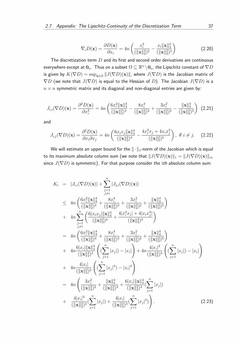
2.7. Appendix: The Lipschitz-Continuity of the Discretization Term 37
∇iD(x) =∂D(x)
∂xi= 4n
(x3i
(‖x‖22)2− xi‖x‖4
4
(‖x‖22)3
)(2.20)
The discretization term D and its first and second order derivatives are continuous
everywhere except at 0n. Thus on a subset Ω ⊆ Rn\0n, the Lipschitz constant of ∇Dis given by K(∇D) = supx∈Ω ‖J(∇D)(x)‖, where J(∇D) is the Jacobian matrix of
∇D (we note that J(∇D) is equal to the Hessian of D). The Jacobian J(∇D) is a
n× n symmetric matrix and its diagonal and non-diagonal entries are given by:
Ji,i(∇D)(x) =∂2D(x)
∂x2i
= 4n
(6x2
i ‖x‖44
(‖x‖22)4− 8x4
i
(‖x‖22)3
+3x2
i
(‖x‖22)2− ‖x‖4
4
(‖x‖22)3
)(2.21)
and
Ji,j(∇D)(x) =∂2D(x)
∂xi∂xj= 4n
(6xixj‖x‖4
4
(‖x‖22)4
−4x3
ixj + 4xix3j
(‖x‖22)3
), if i 6= j. (2.22)
We will estimate an upper bound for the ‖ · ‖1-norm of the Jacobian which is equal
to its maximum absolute column sum (we note that ‖J(∇D)(x)‖1 = ‖J(∇D)(x)‖∞since J(∇D) is symmetric). For that purpose consider the ith absolute column sum:
Ki = |Ji,i(∇D)(x)|+n∑j=1j 6=i
|Jj,i(∇D)(x)|
≤ 4n
(6x2
i ‖x‖44
(‖x‖22)4
+8x4
i
(‖x‖22)3
+3x2
i
(‖x‖22)2
+‖x‖4
4
(‖x‖22)3
)+ 4n
n∑j=1j 6=i
(6|xixj|‖x‖4
4
(‖x‖22)4
+4|x3
ixj|+ 4|xix3j |
(‖x‖22)3
)
= 4n
(6x2
i ‖x‖44
(‖x‖22)4
+8x4
i
(‖x‖22)3
+3x2
i
(‖x‖22)2
+‖x‖4
4
(‖x‖22)3
)+ 4n
6|xi|‖x‖44
(‖x‖22)4
((n∑j=1
|xj|)− |xi|
)+ 4n
4|xi|3
(‖x‖22)3
((n∑j=1
|xj|)− |xi|
)
+ 4n4|xi|
(‖x‖22)3
((n∑j=1
|xj|3)− |xi|3)
= 4n
(3x2
i
(‖x‖22)2
+‖x‖4
4
(‖x‖22)3
+6|xi|‖x‖4
4
(‖x‖22)4
(n∑j=1
|xj|)
+4|xi|3
(‖x‖22)3
(n∑j=1
|xj|) +4|xi|
(‖x‖22)3
(n∑j=1
|xj|3)
). (2.23)

38 Chapter 2. Discrete Tomography with Unknown Intensity Levels
Let X = maxi|xi|. Using the inequalities |xi| ≤ X, ‖x‖44 ≤ nX4 and
∑nj=1 |xj| ≤
nX, we obtain a simple upper bound for all of the absolute column sums, thus an
upper bound for the ‖ · ‖1-norm of the Jacobian:
‖J(∇D)(x)‖1 = maxiKi ≤ 4n
[3X2
(‖x‖22)2
+9nX4
(‖x‖22)3
+6n2X6
(‖x‖22)4
](2.24)
Hence, knowing only the maximal absolute value X and the norm ‖x‖22 we can compute
an upper bound for ‖J(∇D)(x)‖ using Eq. (2.24). This also follows that if on a set
ΩS,M ⊆ Rn, the maximum absolute elements maxi|xi| are upper bounded while
‖x‖22 has a lower bound, then ∇D is Lipschitz continuous on that set, i.e., if
ΩS,M =x ∈ Rn | max
i|xi| ≤M,S ≤ ‖x‖2
2
, (2.25)
then
K(∇D) = supx∈ΩS,M
‖J(∇D)(x)‖ ≤ 4n
[3M2
S2+
9nM4
S3+
6n2M6
S4
]. (2.26)
Now we construct the set of the next possible solutions. Suppose that the current
solution is x and let y = x− (1/K∗(∇C))∇Eα,µ(x). Consider the line segment that
connects x and y:
Λ = `x + (1− `)y | 0 ≤ ` ≤ 1. (2.27)
Since we are looking for a step-length t = 1/(K∗(∇E)) = 1/(K∗(∇C)+µK∗(∇D)),
thus t ≤ 1/K∗(∇C) and after the gradient descent step the next solution x′ will fall
on the line segment Λ. Thus we will compute an upper bound of K(∇D) on Λ. For
that purpose, consider the largest absolute value of the components of the vectors in
Λ, i.e., let M = maxx∈Λmaxi |xi| and the square of the smallest vector norm in
Λ, i.e., let S = minx∈Λ‖x‖22. Since Λ is a line segment, thus M can be computed
considering only its end points x and y:
M = max
maxi|xi|,max
i|yi|
, (2.28)
while S can be computed as the square of the minimal norm of the points on the line
segment Λ:
S =
‖x‖2
2 if k ≤ 0
‖y‖22 if k ≥ 1
‖x + k(y − x)‖22 otherwise,
(2.29)
where k = 〈x,x−y〉‖x−y‖22
and 〈·|·〉 denotes the dot-product operation. It can be easily seen,
that Λ ⊆ ΩS,M , thus an upper bound of K∗(∇D) on Λ is given by Eq. (2.26).

2.7. Appendix: The Lipschitz-Continuity of the Discretization Term 39
In the first step of the proposed method where the initial continuous reconstruction
is obtained by the minimization of E0,0(x) ≡ C(x), setting t = 1/K∗(∇C) as the
gradient descent step size will provide convergence to the global optimum. In the
discretization phase where the objective function Eα,µ is minimized with µ > 0, before
each gradient descent step, M and S can be computed for the current solution x using
Eq. (2.28) and Eq. (2.29), and then K∗(∇D) can be estimated using Eq. (2.26). Then
using step size t∗ = 1/K∗(∇E) = 1/(K∗(∇C)+µK∗(∇D)) ensures that the gradient
descent step will not increase the function value, thus the iterations will converge. In
our experiments, the proposed method provided similar results using this step-length
estimation as with the line search method, we found that the estimation of S and
M before each descent step was computationally less efficient in our implementation.
On the other hand in a parallel implementation, the computation of S and M could
be accelerated, and the step-length t∗ can be considered as an alternative to the line
search.


Chapter 3
Binary Shape Deconvolution Using
Discrete Tomography
In [94], Sharif et al. described a discrete tomography based binary deconvolution al-
gorithm. The size of the point-spread-function (PSF) was restricted to 3× 3 and the
restoration of the projections was handled as a simple linear inverse problem. Moreover,
the method applied the Ryser’s algorithm [88] to reconstruct the shapes, followed by
a further time-consuming step to resolve the switching component ambiguities.
In this chapter a Tikhonov-regularization [101] based method is proposed to de-
convolve the projections of the binary shape. The main advantage of this approach is
that the best value of the regularization parameter can be automatically set using the
L-curve method [44]. In the second step, the binary shape is reconstructed from the de-
convolved projections using efficient network-flow discrete tomography algorithm [15].
The examine the efficiency of the method on synthetic as well as on real images and
compare it to a well-known, widely-used method.
3.1 The Restoration Method
The goal of image restoration is to reconstruct an original image f ∈ Ru×v from its
degraded observation g ∈ Ru×v which is blurred and noisy. The degradation process
(as usually) is modeled as the convolution of the original image with the points-spread-
function (PSF) and the addition of some noise:
g = h ∗ ∗f + n, (3.1)
where h ∈ Rp×q is the point spread function, ∗∗ denotes the 2-dimensional convolution
operator and n ∈ Ru×v is the additive noise. Here we assume that the PSF is known.
Our goal is to restore binary images, such as b ∈ 0, 1u×v. However, in the case of
41

42 Chapter 3. Binary Shape Deconvolution Using Discrete Tomography
⇒
⇒
⇑ ⇓
Figure 3.1: The degradation model and the basic idea of the proposed method. First
three columns: the original binary image, the blurred image and the blurry and noisy
image and their horizontal (top) and vertical (middle) projections. Fourth column:
the method restores the projections of the binary image from the projections of the
degraded image then reconstructs the binary shape.
real images the scaling of the intensity values can be arbitrary. Therefore we introduce
the unknown scale factor s ∈ R and
f = sb (3.2)
in the degradation model Eq. (3.1).
Let denote by f θ the projection vector of an image f along an arbitrary directional
angle θ, i.e., f θ is the discrete approximation of the well-known Radon transform [28]
in direction θ (we simply write f when the actual direction is not important). Here
we take advantage of the following property of the Radon transform: the result of the
Radon transform of a two dimensional convolution is the same as the one dimensional
convolution of the Radon transformed functions, i.e., if g = h ∗ ∗f then g = h ∗ f ,
where ∗ denotes the 1-dimensional convolution operator. A similar relation is true for
the addition. Thus the relationship between the projections of the original and the
degraded images can be expressed as
g = h ∗ f + n. (3.3)
For a direction set Ω = θi|i = 1, . . . , k the proposed method first estimates each
projection f θi of the unknown original image from the projections gθi of the degraded

3.1. The Restoration Method 43
Figure 3.2: A typical L-curve and its curvature. The best trade-off between the norm
of the residual and the norm of the solution is assigned by the maximal curvature value.
image and then as a second step reconstructs f from its estimated projections (see
Fig. 3.1).
3.1.1 Deconvolution of the Projections
In this section we introduce a Tikhonov-regularization [101] based method for the
deconvolution of the projections. Convolution is a linear operation, thus Eq. (3.3) can
be written as
g = Hf + n, (3.4)
where the H matrix represents the convolution operation with the filter h. Since n is
unknown, this system of linear equations is ill-posed and it requires regularization which
penalizes solutions of large norm. The standard version of the Tikhonov regularization
takes the form
fλ = arg minf
‖Hf − g‖22 + λ2‖f‖2
2, (3.5)
where λ is a positive constant, the regularization parameter, that controls the smooth-
ness of the solution. As λ increases the norm of the residual ‖Hfλ− g‖22 also increases
(i.e., fλ becomes less accurate), while the norm of the solution ‖fλ‖22 decreases (i.e.,
fλ becomes smoother). An explicit solution for a given value of λ is given by
fλ = (HTH + λ2I)−1HT g, (3.6)
where I denotes the identity matrix. To determine a suitable value of the regularization
parameter λ we used the so-called L-curve method [44]. The L-curve is the log-log
plot of the norm of the residual and the norm of the solution for different regularization
parameters:
L = (log2 ‖Hfλ − g‖22, log2 ‖fλ‖2
2), λ ≥ 0. (3.7)

44 Chapter 3. Binary Shape Deconvolution Using Discrete Tomography
i = 0 i = 1 i = 10 i = 100
Figure 3.3: The evolution of the estimation of the projection vector during the iteration.
To obtain an optimal trade-off between the two values, the L-curve method proposes
to choose λ∗ which maximizes the curvature κλ of the curve L (see Fig. 3.2). Although
the L-curve method requires for a large set of different λ values to evaluate Eq. (3.6),
it is still computationally efficient approach.
Since the elements of the projection vectors are non-negative we are interested in a
solution of Eq. (3.4) such that f > 0. Unfortunately there is no simple explicit solution
for this problem, but a typical iterative approach can be applied. For that purpose, we
denoted by f+ the version of the vector f in which all negative values were set to 0 .
Let f0 = fλ∗ the initial estimation. In each iteration step the method estimates fi that
approximates f+i−1 (see Fig. 3.3). This can be formulated by the following minimization
problem:
fi = arg minf
‖Hf − g‖22 + λ∗2‖f‖2
2 + ‖f − f+i−1‖2
2 (3.8)
which introduces an additional term to Eq. (3.5) that prefers similarity to the non-
negative version of the previous estimation. This form of the generalized Tikhonov
regularization has an explicit solution:
fi = (HTH + (1 + λ∗2)I)−1(HT g + f+i−1). (3.9)
The iteration ends if ‖fi− fi−1‖22 < ε‖fi−1‖2
2 for an appropriately small ε > 0. The re-
sulting vector f = f+i will be the estimation of the projection vector. The pseudo code
of this algorithm can be found in Algorithm 3. Furthermore the residual ‖Hf − g‖22
approximates n and thus the variance σ2n of the additive noise n can be easily estimated.
3.1.2 Binary Tomographic Reconstruction
In this section we propose a method to reconstruct the binary image from the vectors
f θi using a standard discrete tomography technique. The reconstruction requires the
bθi = f θi/s binary projections. Unfortunately the scale factor s can not be determined
explicitly but the upper and lower bounds of its possible values can be easily estimated.
For that purpose, consider the maximal scaled projection value M = maxθimaxf θi
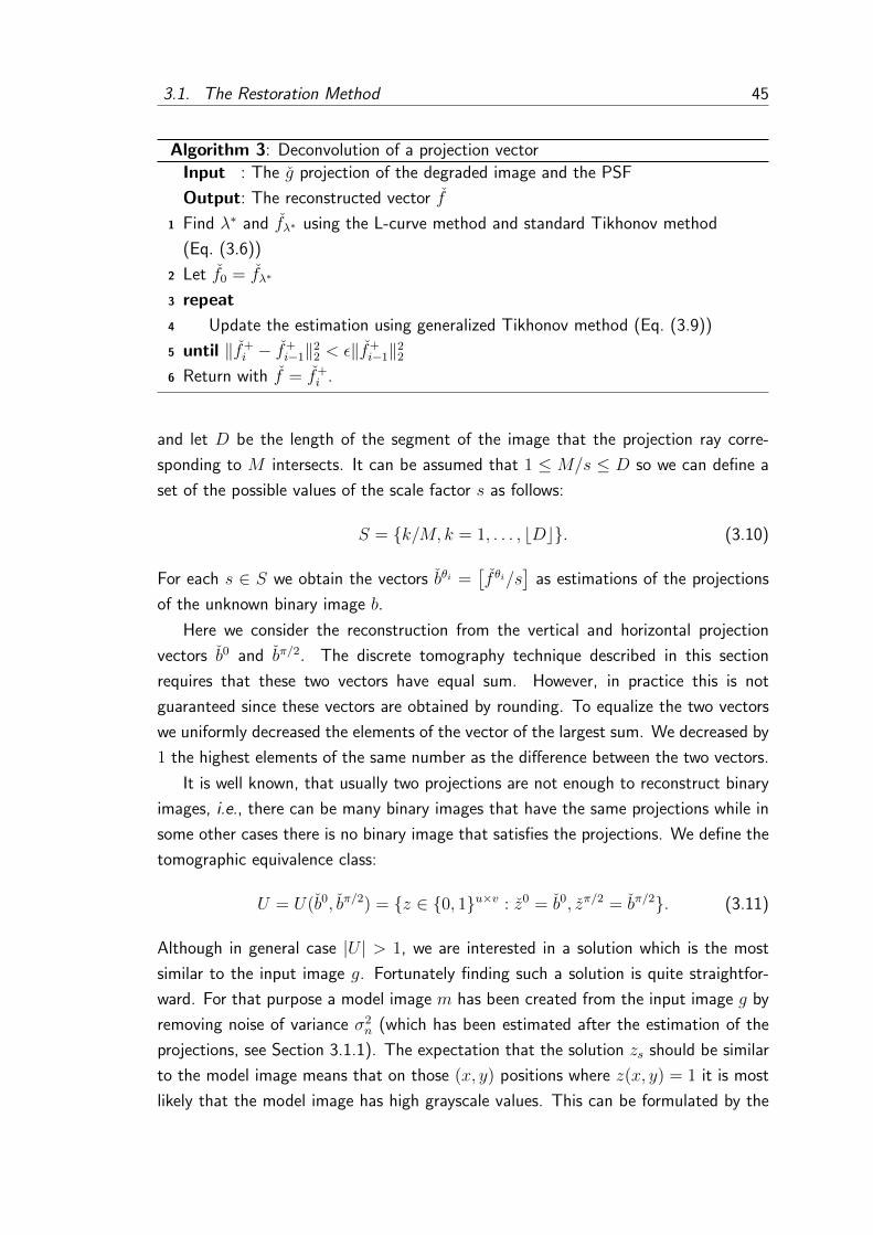
3.1. The Restoration Method 45
Algorithm 3: Deconvolution of a projection vector
Input : The g projection of the degraded image and the PSF
Output: The reconstructed vector f
Find λ∗ and fλ∗ using the L-curve method and standard Tikhonov method1
(Eq. (3.6))
Let f0 = fλ∗2
repeat3
Update the estimation using generalized Tikhonov method (Eq. (3.9))4
until ‖f+i − f+
i−1‖22 < ε‖f+
i−1‖225
Return with f = f+i .6
and let D be the length of the segment of the image that the projection ray corre-
sponding to M intersects. It can be assumed that 1 ≤ M/s ≤ D so we can define a
set of the possible values of the scale factor s as follows:
S = k/M, k = 1, . . . , bDc. (3.10)
For each s ∈ S we obtain the vectors bθi =[f θi/s
]as estimations of the projections
of the unknown binary image b.
Here we consider the reconstruction from the vertical and horizontal projection
vectors b0 and bπ/2. The discrete tomography technique described in this section
requires that these two vectors have equal sum. However, in practice this is not
guaranteed since these vectors are obtained by rounding. To equalize the two vectors
we uniformly decreased the elements of the vector of the largest sum. We decreased by
1 the highest elements of the same number as the difference between the two vectors.
It is well known, that usually two projections are not enough to reconstruct binary
images, i.e., there can be many binary images that have the same projections while in
some other cases there is no binary image that satisfies the projections. We define the
tomographic equivalence class:
U = U(b0, bπ/2) = z ∈ 0, 1u×v : z0 = b0, zπ/2 = bπ/2. (3.11)
Although in general case |U | > 1, we are interested in a solution which is the most
similar to the input image g. Fortunately finding such a solution is quite straightfor-
ward. For that purpose a model image m has been created from the input image g by
removing noise of variance σ2n (which has been estimated after the estimation of the
projections, see Section 3.1.1). The expectation that the solution zs should be similar
to the model image means that on those (x, y) positions where z(x, y) = 1 it is most
likely that the model image has high grayscale values. This can be formulated by the

46 Chapter 3. Binary Shape Deconvolution Using Discrete Tomography
Figure 3.4: Associated network for a 3×3 case. The supply and demand values for the
source nodes Si and the sink nodes Tj are given by the vectors b0 and bπ/2 respectively.
Each of the edges has a flow capacity equal to 1 while the flow costs are given by the
model image m ∈ R3×3.
following minimization problem:
zs = arg minz∈U
(−∑x,y
z(x, y)m(x, y)
). (3.12)
This way the reconstruction problem can be traced back to the minimum cost maximal
flow (MCMF) problem [15]. In this network the supply and demand nodes are repre-
senting the projection vectors while the edges are representing the image pixels (see
Fig. 3.4). The edge Sx → Ty corresponding to the (x, y) pixel has a flow capacity equal
to 1 and a flow cost equal to −m(x, y). The minimum cost maximal flow can be found
in polynomial time [80] and it determines the solution zs of the discrete tomography
problem. The pixel zs(x, y) gets a value of 1, if and only if the flow passes through the
edge Sx → Ty. As it has been noted previously in some cases the projections can not
be satisfied, i.e., U is empty. In such cases we simply discard the current scale factor
and the corresponding projections. We also note that the original input image g could
also be used as model image, however the results would be somewhat more noisy.
For different scale factors s ∈ S the method finds different binary solutions zs (see
Fig. 3.5). To choose an optimal solution z, the method compares each zs to the input

3.2. Experiments and Comparison 47
s = 0.64 s = 0.92 s = 1.07 s = 1.21 s = 1.32
Figure 3.5: Reconstruction results for different s ∈ S scale values.
image g in least-squares sense
z = arg minzs
‖s(h ∗ ∗zs)− g‖2. (3.13)
It should be noted that theoretically it is not impossible that |U | = 0 for each scale
factor s ∈ S. In this case the proposed method could not provide any solution.
However in practice we found that U containes at least one solution for most of s ∈ S.
The pseudo code of the algorithm can be found in Algorithm 4. As for the time
complexity of the overall algorithm, the reconstruction of the projections require a
matrix invertion in each iteration step which has a polynomial time consumption while
the reconstruction of the binary shapes for each scale factor s ∈ S using the MCMF
approach has also polynomial time complexity. Hence the overall method is computa-
tionally efficient.
3.2 Experiments and Comparison
We examined the performance of the proposed method on synthetic dataset of images
of 62 alphanumeric characters of size 59× 59 pixels and their 1550 degraded versions.
Each image was blurred by Gaussian filters with standard deviations σ = 0, 1, . . . , 5.
Algorithm 4: Shape restoration using discrete tomography
Input : The degraded grayscale image g and the PSF h
Output: The reconstructed binary image z
Restore the projections f 0 and fπ/2 using the method described in Section 3.1.11
foreach s ∈ S do2
Reconstruct the binary image zs from the vectors b0 =[f 0/s
]and3
bπ/2 =[fπ/2/s
]using the method described in Section 3.1.2
end4
Return with z = zs according to Eq. (3.13)5

48 Chapter 3. Binary Shape Deconvolution Using Discrete Tomography
Richardson-Lucy method
σ 5dB 2.5dB 0dB -2.5dB -5dB
1.0 9.93 12.66 15.94 21.78 30.58
2.0 12.01 14.57 17.80 23.99 31.21
3.0 10.30 13.06 16.85 21.96 29.98
4.0 14.47 16.98 20.30 26.44 35.26
5.0 21.28 24.04 27.07 32.87 41.44
Proposed method
σ 5dB 2.5dB 0dB -2.5dB -5dB
1.0 10.83 12.31 14.44 18.88 24.15
2.0 14.67 15.69 17.19 20.80 22.61
3.0 17.41 18.34 19.94 21.66 24.58
4.0 21.53 23.38 25.17 27.53 29.44
5.0 26.47 28.43 30.90 32.50 35.75
Table 3.1: Test results on the synthetic dataset of the Richardson-Lucy method and
the proposed method. The average δ measures on 62 alphanumeric characters for
different levels of blur and SNR are shown. The cases when the proposed method
provided better results are depicted in bold.
White noises of different levels was added to each blurred image to implement signal-
to-noise ratios of 5, 2.5, 0, -2.5, -5 dB. The reconstruction results were evaluated using
the following normalized symmetric difference
δ =|B M Z||B|+ |Z|
· 100%, (3.14)
where B and Z denote the set of the foreground pixels of the original image b and the
reconstructed image z respectively.
For comparison, we have chosen the Richardson–Lucy algorithm [84] because this
method also assumes that the PSF is known and does not require an estimation of
the strength of the noise. On the other hand this method was developed for grayscale
images thus thresholding is required. In our experiments Otsu [81] thresholding pro-
vided the best solutions. To improve the results of both methods, small isolated pixel
groups has been removed from the reconstructed images by the following way. First,
a morphological closing has been applied to connect regions and isolated pixels that
are close to each other. Then 8-connected pixel groups containing at most a certain

3.2. Experiments and Comparison 49
Figure 3.6: Example reconstruction results on synthetic images. First three rows:
The original binary shapes, the blurred images, and the blurred and noisy version (from
top to middle). Fourth and fifth rows: The results of the Richardson-Lucy method
and the proposed method respectively.
number of pixels has been removed. Finally, a logical AND operation with the original
shape has been applied to undo the morphological closing. It has to be noted that
the Richardson-Lucy method produced much more of such artifacts. The summary
of the test results is shown in Table 3.1. It can be seen that the proposed method
provided better results in low SNR cases. This is due to the L-curve based estimation
of the regularization parameter which implicitly gives a robust estimation of the level
of the noise. On the other hand, in higher SNR cases the 2-dimensional deconvolution
methods (like the Richardson–Lucy algorithm) can provide more accurate restorations.
The Richardson–Lucy algorithm requires a couple of Fourier transforms in each
iteration step, thus for fixed number of iterations, its time complexity isO (uv log (uv)).
As we discussed in the previous section, the proposed method has a polynomial time
complexity. We implemented our method in Matlab, but the network-flow algorithm
was written in C. This inefficient mixed solution resulted longer running times (an
average of ≈ 5 sec.), while the Richardson–Lucy algorithm was very fast (below 0.1
sec.). However a more efficient implementation of our method is probably feasible.

50 Chapter 3. Binary Shape Deconvolution Using Discrete Tomography
Figure 3.7: Example results on letters extracted from out-of-focus document images
taken with EDoF camera. The input images are shown in the first row. The recon-
struction results of the Richardson-Lucy method can be found in the second row and
the results of the proposed method are in the third row.
3.2.1 Experiments on Real Out of Focus Images
Nowadays optical character recognition (OCR) is one of the most important func-
tionalities of mobile devices. Nevertheless many modern devices are equipped with
fixed-focus or full-focus (Extended Depth of Field - EDoF) lens. While these cam-
eras in many cases provide better image quality than many auto-focus cameras, they
usually can not be used for OCR because the images of A4 pages or business cards
taken from a distance about 20 cm are out-of-focus. Therefore the enhancement of
such images is an interesting task. We extracted a set of letters from images of A4
papers taken with an EDoF camera. Gaussian filters has been used as PSFs and their
radius has been determined empirically. The results of the Richardson-Lucy method
and the proposed method are shown in Fig. 3.7. It can be observed that the proposed
method provided better results in same cases , thus it can be regarded as a promising
alternative. We note that it is not clear that Gaussian filter approximates the best the
out-of-focus effect. Disk shaped low-pass filters was also tested but while we obtained
similar results with the proposed method, the Richardson-Lucy method provided much
weaker restoration.
3.3 Summary
In this chapter we described a binary tomography based image restoration method.
The first step of the method restores the projections of the shape using 1-dimensional
deconvolution while the second step reconstructs the binary image using a discrete
tomography technique. The main advantage of the method is that it does not require
parameter setting or prior knowledge like the estimation of the signal-to-noise ratio.
The optimal trade-off between the residual and the accuracy is determined automati-

3.3. Summary 51
cally using L-curve method. Numerical experiments on synthetic images showed that
the method is robust to the level of the noise and can outperform a widely-used method
in low SNR cases. The efficiency of the method has also been demonstrated on real
alphanumeric images taken with fixed-focus camera.
In the described version of the algorithm, the intensity level of the shapes is found
by performing tomography reconstructions assuming different possible values. For each
value, we perform a tomographic reconstruction, and the best intensity level is found by
comparing the result to the input image. This procedure is required because the applied
binary tomographic technique assumes that the intensity levels are known (i.e., 0 for
the background and 1 for the shape pixels). Furthermore, the described reconstruction
method is restricted to two projections.
Therefore in the future research, the algorithm could be improved by applying
other tomography reconstruction algorithms. For example, the method described in
Chapter 2 can deal with the problem of unknown intensity levels, and moreover, it
allows to use more than two projections, which would probably improve the accuracy
of the restoration.


Chapter 4
Nonlinear Registration of Binary
Shapes
In this chapter, a general registration framework is proposed which can be used to
estimate the parameters of nonlinear transformations between binary shapes without
established point correspondences. The basic idea of the method is to set up a system
of nonlinear equations by integrating a set of linearly independent nonlinear functions
over the image domains. The system is then solved using the classical Levenberg-
Marquardt algorithm [66]. The framework is applied to different nonlinear transforma-
tion models (e.g., planar homography, polynomial or thin plate spline transformations),
and the performance and robustness of the method is demonstrated using tests on large
set of synthetic images. The method has also been successfully applied in the case
of different real-world applications, e.g., registration of X-ray images, traffic signs and
handwritten characters, and the visual inspection of printed signs on tubular structures.
4.1 A Parametric Reconstruction Framework
In this section we introduce a novel general registration method. Suppose that
ϕ : R2 → R2 is a differentiable and invertible transformation (see Fig. 4.1), and its
inverse is also differentiable (i.e., ϕ is a diffeomorphism). Our goal is to estimate its pa-
rameters with which the transformation aligns the shapes. Let the corresponding point
coordinates on the template and observation shapes denoted by x = [x1, x2]T ∈ R2
and y = [y1, y2]T ∈ R2. Then the identity relation between these points can be written
as followings:
y = ϕ(x) ⇔ x = ϕ−1(y), (4.1)
where ϕ−1 : R2 → R2 is the corresponding inverse transformation.
Consider the shapes as their characteristic function 1 : R2 → 0, 1, where 0 and
53

54 Chapter 4. Nonlinear Registration of Binary Shapes
Figure 4.1: Problem statement: Estimation of the parameters of the aligning transfor-
mation (in this case a planar homography transformation) using the segmented versions
of the images.
1 denotes the background and the foreground points respectively. If the template and
the observation shapes are denoted by 1t and 1o, then
1o(y) = 1o
(ϕ(x)
)= 1t(x), (4.2)
since x and y are corresponding point coordinates.
Classical correspondence based registration approaches would set up a system of
equations from Eq. (4.1), of which solution gives the aligning parameters. Herein,
however, we are looking for a correspondenceless solution. We can obtain a relation
between the area of the shapes by integrating out individual point correspondences
over the foreground regions and applying the integral transformation y = ϕ(x), dy =
|Jϕ(x)| dx: ∫R2
1o(y)dy =
∫R2
1t(x) |Jϕ(x)| dx, (4.3)
where the Jacobian |Jϕ| : R2 → R of the transformation ϕ is given by:
|Jϕ(x)| =
∣∣∣∣∣∣∂ϕ1
∂x1
∂ϕ1
∂x2
∂ϕ2
∂x1
∂ϕ2
∂x2
∣∣∣∣∣∣ . (4.4)
The value of the Jacobian |Jϕ(x)| gives the area changing caused by the transformation
ϕ at the point x (i.e., the measure of the transformation). We note that in the case of
affine (linear) transformations this measure is constant, and can be estimated simply

4.1. A Parametric Reconstruction Framework 55
as the ratio of the areas of the shapes [31]. However the Jacobian of a nonlinear
transformation is a non-constant function of the point coordinates.
Note that the effect of the multiplication with the characteristic functions basically
only restricts the integral domains to the foreground regions. Let the foreground regions
of the template and observation shapes denoted by Ft = x ∈ R2|1t(x) = 1 and
Fo = y ∈ R2|1o(y) = 1. Thus∫R2
1o(y)dy =
∫Fody, (4.5)
and Eq. (4.3) can be written as∫Fody =
∫Ft|Jϕ(x)| dx. (4.6)
Thus we obtained an equation with unknowns corresponding to the parameters of the
transformation (e.g., in the case of a planar homography, the H11, . . . , H32 parameters,
see Section 4.2.1). Obviously, the left hand side of the equation gives the area of the
observation, while the right hand side gives the area of the transformed template.
Thus Eq. (4.6) expresses the identity of these areas, i.e., that |ϕ(Ft)| = |Fo|. Since
generally the transformation ϕ has more then 1 parameters (or degree of freedom),
only one equation is not enough to estimate these unknowns.
Additional constrains can be obtained by multiplying Eq. (4.1) and Eq. (4.2):
y1o(y) = ϕ(x)1t(x). (4.7)
Integrating both sides gives an equation similar to Eq. (4.6):∫Fo
ydy =
∫Ftϕ(x) |Jϕ(x)| dx. (4.8)
The transformation ϕ can be decomposed as
ϕ(x) = [ϕ1(x), ϕ2(x)]T , (4.9)
where ϕ1, ϕ2 : R2 → R are the coordinate functions. Thus the integrands in Eq. (4.8)
are (two dimensional) vectors and the values of the integrals are also vectors. Thus
Eq. (4.8) can be decomposed into a system of two equations using these coordinate
functions: ∫Foyidy =
∫Ftϕi(x) |Jϕ(x)| dx, i = 1, 2. (4.10)
Although these equations give additional contrains, this system of equation is still not
enough to estimate all of the unknown parameters of ϕ.

56 Chapter 4. Nonlinear Registration of Binary Shapes
ω from Eq. (4.41) ω from Eq. (4.42) ω from Eq. (4.43)
Figure 4.2: The effect of various ω functions. Top: the generated coloring of a binary
shape. Bottom: the corresponding volumes.
4.1.1 Construction of the System of Equations
To obtain more equations, note, that the identity relation in Eq. (4.1) remains valid if
we apply a function ω : R2 → Rn, (n ≥ 1) on both sides of the equation [30, 76, 75]:
ω(y) = ω(ϕ(x)) ⇔ ω(x) = ω(ϕ−1(y)). (4.11)
In a similar way as in the case of Eq. (4.8), we can integrate on both sides and obtain
the following equation:∫Foω(y)dy =
∫Ftω(ϕ(x)) |Jϕ(x)| dx. (4.12)
The basic idea of the proposed method is to generate a sufficient number of equations
using a set of linearly independent ω functions. Since an equation set up using ω :
R2 → Rn (n > 1) can be decomposed into n equations (similarly to Eq. (4.10)), we
can assume that n = 1 without any restriction.
Suppose that ϕ has k parameters and let ωi : R2 → R, (i = 1, . . . , `) the set
of applied functions. To solve for all unknowns, we need at least k equations, hence
` ≥ k. Thus we can obtain the following system of equations∫Foωi(y)dy =
∫Ftωi(ϕ(x)
)|Jϕ(x)| dx, i = 1, . . . , `, (4.13)
where each ωi function provides one new equation. Each applied ωi function can be
considered as a coloring of the shape (see Fig. 4.2) and the integrals in Eq. (4.13) give
the volumes of the ωi functions over the area of the shape. The equations thus match
these volumes.

4.2. The Studied Deformation Models 57
Original shape ϕ(x) = [x1+ce− (x21+x
22)
2σ2 , x2]T ϕ(x) = [x2
2+x1, x21+x2]
T
Figure 4.3: Example deformation fields
Each equation provides additional constraints. The solution of this system gives
the estimation of the parameters of the aligning transformation. Unfortunately the
algebraic independence of the equations can not be garanteed. It can be easily seen,
however, that the linear independency of the ωi functions is an important criterion,
which can be verified much easier. Therefore, in pratice, we propose to apply a set of
linearly independent nonlinear ωi functions.
4.2 The Studied Deformation Models
In this section we introduce the transformation models that has been studied in our
experiments. We note that, while on grayscale (or color) images most of the trans-
formation models cause visible deformation, in the case of binary images, the effect
of some transformations is not always observable (i.e., on binary images the transfor-
mation is not always bijective, see Fig. 4.3). Herein we focus on some such a widely
used transformation classes, but the framework can be applied to any diffeomorphic
transformation. All we need to adopt a transformation model into our framework are
the formular description of the transformation ϕ and its Jacobian |Jϕ(x)|.
4.2.1 Planar Homography
Planar homography is the projective transformation between the images of the same
planar object. It plays an important role in computer vision. The most simple method
to estimate its parameters traces back the problem to the solution of a system of linear
equations. Its coefficients are determined by the coordinates of point correspondences.
The solution requires at least 4 point correspondences, but an overdetermined system
solved in the least-squares sense gives more accurate result in spite of the inaccurate
coordinates. A survery of planar homography estimation techniques can be found in [2].

58 Chapter 4. Nonlinear Registration of Binary Shapes
Figure 4.4: Example perspective distortion
In many cases, when the pespective distortion is weak, affine transformation model is
used to approximate the planar homography or to provide an initial estimation [54].
Planar homography is a projective transformation (see Fig. 4.5 and Fig. 4.4) which
can be given as a linear transformation on the projective plane P2 using the
H =
H11 H12 H13
H21 H22 H23
H31 H32 1
(4.14)
3 × 3 non-singular (|H| 6= 0) matrix. Since such a projective transformation has
8 degree of freedom, we can assume without any restriction that H33 = 1. Then
the transformation between the corresponding points x′ = [x′1, x′2, x′3]T ∈ P2 and
y′ = [y′1, y′2, y′3]T ∈ P2 of the template and the observation shapes is given by
y′ = Hx′ ⇔ x′ = H−1y′ . (4.15)
The Euclidean coordinates y = [y1, y2]T ∈ R2 of the homogeneous point y′ =
[y′1, y′2, y′3]T ∈ P2 are obtained by applying the perspective division:
y1 =y′1y′3
=H11x1 +H12x2 +H13
H31x1 +H32x2 + 1≡ h1(x)
y2 =y′2y′3
=H21x1 +H22x2 +H23
H31x1 +H32x2 + 1≡ h2(x) , (4.16)
where hi : R2 → R. Thus, while planar homography is a linear transformation in the
projective plane P2, it becomes nonlinear in the Euclidian plane R2. Let the nonlinear
transformation corresponding to H denoted by h : R2 → R2, h(x) =(h1(x), h2(x)
)T.
Thus Eq. (4.1) can be written as
y = ϕ(x) ≡ h(x) ⇔ x = h−1(y), (4.17)
where h−1 : R2 → R2 a H−1 is the inverse transformation corresponding to the inverse
matrix. The Jacobian |Jh| : R2 → R is given by
|Jh(x)| =
∣∣∣∣∣∣∂h1∂x1
∂h1∂x2
∂h2∂x1
∂h2∂x2
∣∣∣∣∣∣ =|H|
(H31x1 +H32x2 + 1)3 . (4.18)

4.2. The Studied Deformation Models 59
Figure 4.5: Projective transformations. Left: the images of the circular shape on
the planes P and Q are related by a center-point projection. Right: The planar
homography as the relation between two images of the same plane π taken with
different cameras. (Figure from: [57], [83])
4.2.2 The Taylor Series Expansion of Planar Homography
In the case of planar homography, the integrands in Eq. (4.13) can be approximated by a
Taylor series expansion and this way we can obtain polynomial equations. For example,
consider the term ωi(h(x)) |Jh(x)|, If ωi is polynomial, then both the numerator and
the denominator of ωi(h(x)) will be also polynomial and remains a polynomial when
multiplied by |Jh(x)|. Thus
ωi(h(x)) |Jh(x)| = p(H1, . . . , H6)χ(H7, H8), (4.19)
where p is a polynom, while χ is the remaining non-polynomial term. For example
assuming the ωi set from Eq. (4.41), we get
χ(H7, H8) =1
(H7x1 +H8x2 + 1)3+n+m. (4.20)
where n and m are the exponents in ωi. Since p is polynomial, in order to obtain a
polynomial approximation of the whole term ωi(h(x)) |Jh(x)|, we only need to rewrite
χ(H7, H8) in its nth order multivariate Taylor series form. Let us denote the nth order
Taylor series expanson of the function f : Rk → R about the point (a1, . . . , ak) by
T nf(a1,...,ak). Then χ(H7, H8) can be approximated as follows:
χ(H7, H8) ≈ T nχ(0,0), (4.21)
and thus the whole integrand can be rewritten as:
ωi(h(x)) |Jh(x)| ≈ p(H1, . . . , H6)T nχ(0,0). (4.22)
Substituting each integrand in Eq. (4.37) with the Taylor series expansion approxima-
tion, we obtain a system of polynomial equations. This increases the computational
efficiency, as discussed in Section 4.2.3. In our experiments we obtained good results
with n = 5.
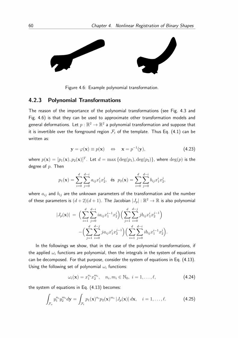
60 Chapter 4. Nonlinear Registration of Binary Shapes
Figure 4.6: Example polynomial transformation.
4.2.3 Polynomial Transformations
The reason of the importance of the polynomial transformations (see Fig. 4.3 and
Fig. 4.6) is that they can be used to approximate other transformation models and
general deformations. Let p : R2 → R2 a polynomial transformation and suppose that
it is invertible over the foreground region Ft of the template. Thus Eq. (4.1) can be
written as:
y = ϕ(x) ≡ p(x) ⇔ x = p−1(y), (4.23)
where p(x) = [p1(x), p2(x)]T . Let d = max deg(p1), deg(p2), where deg(p) is the
degree of p. Then
p1(x) =d∑i=0
d−i∑j=0
aijxi1x
j2, es p2(x) =
d∑i=0
d−i∑j=0
bijxi1x
j2,
where aij and bij are the unknown parameters of the transformation and the number
of these parameters is (d+ 2)(d+ 1). The Jacobian |Jp| : R2 → R is also polynomial
|Jp(x)| =( d∑i=1
d−i∑j=0
iaijxi−11 xj2
)( d∑j=1
d−j∑i=0
jbijxi1x
j−12
)
−( d∑j=1
d−j∑i=0
jaijxi1x
j−12
)( d∑i=1
d−i∑j=0
ibijxi−11 xj2
).
In the followings we show, that in the case of the polynomial transformations, if
the applied ωi functions are polynomial, then the integrals in the system of equations
can be decomposed. For that purpose, consider the system of equations in Eq. (4.13).
Using the following set of polynomial ωi functions:
ωi(x) = xni1 xmi2 , ni,mi ∈ N0, i = 1, . . . , `, (4.24)
the system of equations in Eq. (4.13) becomes:∫Foyni1 y
mi2 dy =
∫Ftp1(x)nip2(x)mi |Jp(x)| dx, i = 1, . . . , `. (4.25)

4.2. The Studied Deformation Models 61
Figure 4.7: Example thin plate spline transformation.
The left hand side of the equations are independent of the parameters of the trans-
formations and can be computed using only the pixel coordinates of the observation
shape. Futhermore since p1(x), p2(x) and |Jp(x)| are polynomials, thus the right hand
sides are also polynomial:∫Ftp1(x)nip2(x)mi |Jp(x)| dx =
∫Ft
ci∑q=0
ci−q∑r=0
tiqrxq1x
r2dx =
ci∑q=0
ci−q∑r=0
tiqr
∫Ftxq1x
r2dx,
(4.26)
where ci = d(ni+mi)+d(d−1) is the order of the polynomial in the ith equation,
while tiqr is a polynomial expression that consists of the parameters of p. Therefore
Eq. (4.26) is a polynomial system of equations, in which the integrals∫Ft x
q1x
r2dy are
independent of the transformation parameters, they have to be computed only once,
in the beginning of the registration process, which highly increases the computational
efficiency of the method.
4.2.4 Thin Plate Spline
The Thin Plate Spline (TPS) model is widely used to approximate general non-rigid
deformations [38]. Let a set of control points ck ∈ R2 and corresponding coefficients
(weights) aij, wki ∈ R, i = 1, 2, j = 1, . . . , 3, k = 1, . . . , K. Then
si(x) = ai1x1 + ai2x2 + ai3 +K∑k=1
wkiQ(||ck − x||), i = 1, 2, (4.27)
where Q : R→ R is the so called radial basis function:
Q(r) = r2 log r2. (4.28)
The physical analogy of this model is a bended thin metal plate. Additional constraints
are proposed to avoid unwanted global effects, such as the movement and the rotation
of the plate under the imposition of the loads [118]:
K∑k=1
wik = 0,K∑k=1
ckiwki = 0, i = 1, 2. (4.29)

62 Chapter 4. Nonlinear Registration of Binary Shapes
Figure 4.8: Coverage of transformed shapes of ≈ 1500 synthetic observations during
the minimization process. Pixel values represent the number of intermediate shapes
that included a particular pixel. For reference, we also show the circle with radius√
22
used for normalization.
Now s(x) = [s1(x), s2(x)]T ,
y = ϕ(x) ≡ s(x) ⇔ x = s−1(y) (4.30)
defines a transformation with 6 + 2K parameters (6 affine parameter aij and 2K
coefficients wki for the control points).
The Jacobian |Js| : R2 → R of the transformation is given by:
|Js(x)| =
∣∣∣∣∣∣∂s1∂x1
∂s1∂x2
∂s2∂x1
∂s2∂x2
∣∣∣∣∣∣ , (4.31)
where∂si∂xj
= aij +K∑k=1
wik[− 2(ckj − xj)
(1 + log(||ck − x||)
)]. (4.32)
4.3 Implementational Details
It is required to avoid extreme (large or small) numerical values of the integrals. It
can be done by applying some normalization on both the pixel coordinates and the ωi
functions. For that purpose, we normalized the coordinates of both shapes into the
square [−0.5, 0.5]× [−0.5, 0.5] and chose ωi with a range limited to the interval (e.g.,
[−1, 1]).
Despite of these normalizations, the integrals in our equations could take values of
different range of magnitude yielding a different contribution from each equation to

4.3. Implementational Details 63
h−11 (y) = x1 =
(H22 −H32H23)y1 − (H12 −H32H13)y2 +H23H12 −H22H13
(H32H21 −H31H22)y1 − (H32H11 −H31H12)y2 +H22H11 −H21H12
h−12 (y) = x2 =
−(H21 −H31H23)y1 + (H11 −H31H13)y2 − (H23H11 −H21H13)
(H32H21 −H31H22)y1 − (H32H11 −H31H12)y2 +H22H11 −H21H12
|Jh−1(y)| =|H|2(
(H32H21 −H31H22)y1 − (H32H11 −H31H12)y2 +H22H11 −H21H12
)3(4.36)
the objective function value in the optimization process. To overcome this issue, we
also normalized the equations by dividing the integrals with an appropriate constant.
We found experimentally (see Fig. 4.8), that the transformations occurring during the
least-squares minimization process do not transform the shapes out of a circle with
center in the origin and a radius√
22
(i.e., the circumscribed circle of the unit square).
We thus adopt the following constant
Ni =
∫‖x‖≤
√2
2
|ωi(x)|dx, (4.33)
and the normalized version of Eq. (4.13) becomes∫Fo ωi(y)dy
Ni
=
∫Ft ωi
(ϕ(x)
)|Jϕ(x)| dx
Ni
, i = 1, . . . , `. (4.34)
4.3.1 Numerical Implementation
The system of equations in Eq. (4.13) has been constructed in the continuous space,
in practice, however, we have limited resolution digital images. Therefore the integrals
can only be approximated by finite sums over the foreground pixels. This approximation
obviously introduces a negligible error into the equations. Let us denote by Ft and Fo
the finite pixel sets corresponding to the continuous pixel regions Ft and Fo. Then
Eq. (4.34) can be approximated by the following system of equations:
1
Ni
∑y∈Fo
ωi(y) =1
Ni
∑x∈Ft
ωi(ϕ(x)
)|Jϕ(x)| , i = 1, . . . , `. (4.35)
This system of equations can be supplemented with further equations depending on
the transformation model. These additional equations are either to improve numerical
stability (like in the case of planar homography) or to enforce additional constraints
required by the model (e.g., thin plate spline).
Planar homography: Since the inverse of a planar homography is also a planar
homography, each equation of Eq. (4.35) can also be written in three alternative forms

64 Chapter 4. Nonlinear Registration of Binary Shapes
by making use of the corresponding inverse transformation h−1 and the reverse integral
transformation x = h−1(y), dx = |Jh−1(y)| dy:
1
Ni
∑x∈Ft
ωi(x) =1
Ni
∑y∈Fo
ωi(h−1(y)
)|Jh−1(y)|
1
Ni
∑x∈Ft
ωi(x) |Jh(x)| =1
Ni
∑y∈Fo
ωi(h−1(y)
)1
Ni
∑x∈Ft
ωi(h(x)
)=
1
Ni
∑y∈Fo
ωi(y) |Jh−1(y)| . (4.37)
where h−1 and |Jh−1(y)| are defined in Eq. (4.36). While these equations are equivalent
to the original one, including them provides additional constraints and thus helps the
optimizer to find the optimal solution.
Thin plate spline: In the case of this transformation model, the number of required
equations depends on the number of the control points. Furthermore, the constraints
in Eq. (4.29) has to be included in the system of equations.
4.3.2 Solution and Complexity
The parameters of the aligning transformations are obtained as the solution of the
system of equations. While the equations are nonlinear, we found that it can be solved
efficiently by Levenberg-Marquardt algorithm [66] in least-squares sense. This method
is commonly applied in function fitting, thus in the case of a function f : Rk → R`, it
is suitable to solve:
minx
∑i=1
(fi(x)
)2, x ∈ Rk. (4.38)
The system of equations in Eq. (4.13) can be simply transformed into such a mini-
mization problem, by substituting its two sides. Thus we obtain an objective function
of class Rk → R`, where k is the number of the transformation parameters and ` is
the number of equations (i.e., the number of the applied ωi functions). As an iterative
optimizing method, the Levenberg-Marquardt method requires an initial solution. We
found, that the parameter vector corresponding to the identity transformation is appro-
priate for that purpose. For example, in the case of planar homography it is the values
of the H0 = I3×3 identity matrix. On the other hand, in many cases one can find
a better initial solution. For example the scaling between the shapes can be initially
approximated as the ratio of the shape areas. For example, for planar homography
H0 =
s0 0 0
0 s0 0
0 0 1
, where s0 =
√M
N, (4.39)
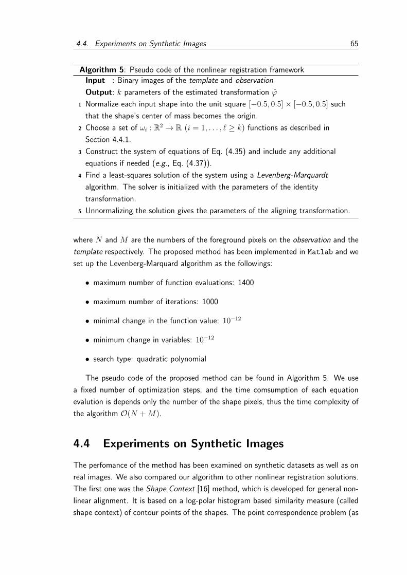
4.4. Experiments on Synthetic Images 65
Algorithm 5: Pseudo code of the nonlinear registration framework
Input : Binary images of the template and observation
Output: k parameters of the estimated transformation ϕ
Normalize each input shape into the unit square [−0.5, 0.5]× [−0.5, 0.5] such1
that the shape’s center of mass becomes the origin.
Choose a set of ωi : R2 → R (i = 1, . . . , ` ≥ k) functions as described in2
Section 4.4.1.
Construct the system of equations of Eq. (4.35) and include any additional3
equations if needed (e.g., Eq. (4.37)).
Find a least-squares solution of the system using a Levenberg-Marquardt4
algorithm. The solver is initialized with the parameters of the identity
transformation.
Unnormalizing the solution gives the parameters of the aligning transformation.5
where N and M are the numbers of the foreground pixels on the observation and the
template respectively. The proposed method has been implemented in Matlab and we
set up the Levenberg-Marquard algorithm as the followings:
• maximum number of function evaluations: 1400
• maximum number of iterations: 1000
• minimal change in the function value: 10−12
• minimum change in variables: 10−12
• search type: quadratic polynomial
The pseudo code of the proposed method can be found in Algorithm 5. We use
a fixed number of optimization steps, and the time comsumption of each equation
evalution is depends only the number of the shape pixels, thus the time complexity of
the algorithm O(N +M).
4.4 Experiments on Synthetic Images
The perfomance of the method has been examined on synthetic datasets as well as on
real images. We also compared our algorithm to other nonlinear registration solutions.
The first one was the Shape Context [16] method, which is developed for general non-
linear alignment. It is based on a log-polar histogram based similarity measure (called
shape context) of contour points of the shapes. The point correspondence problem (as

66 Chapter 4. Nonlinear Registration of Binary Shapes
Eq. (4.41) Eq. (4.42) Eq. (4.43)
Eq. (4.44) Eq. (4.45) Eq. (4.46)
Figure 4.9: Plots of tested ωi function sets.
an assignment problem) is then solved by the Hungarian method. The main advantage
of this approach that it does not require intensity information. Its demo implementation
is available on the internet [89], we set the parameters empirically to their optimal value
( beta init=30, n iter=30, r=1).
The registration results were evaluated using two different error measures. The δ
measure gives the normalized symmetric difference of shapes, while ε measures the
distance between the true ϕ and the estimated ϕ transformation:
δ =|Fr M Fo||Fr|+ |Fo|
· 100%, ε =1
|Ft|∑x∈Ft
‖ϕ(x)− ϕ(x)‖, (4.40)
where Fr, Ft and Fo are the sets of the object pixels of the registered, the template,
and the observation shapes, while M denotes the symmetric difference. Obviously, ε
can be used only in the case of synthetic tests, where the original parameters of the
transformation used to generate the distorted shape are known. To examine the test
results, the median, mean, and standard deviation of the error measures have been
calculated.
4.4.1 Comparison of Different ω Functions
Theoretically any set of linearly independent ωi functions could be used to set up the
system of equations in Eq. (4.13). Obviously, ωi must be an integrable function over
the finite domains Fo and Ft, and the equations should be properly normalized. In
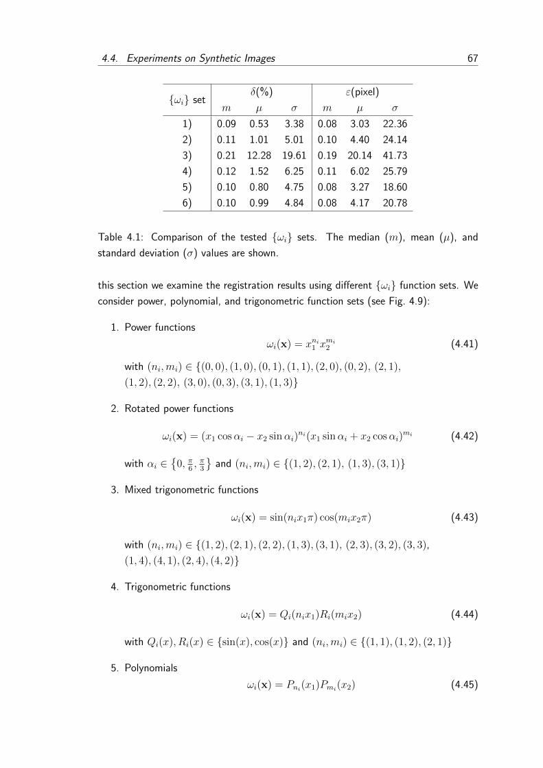
4.4. Experiments on Synthetic Images 67
ωi setδ(%) ε(pixel)
m µ σ m µ σ
1) 0.09 0.53 3.38 0.08 3.03 22.36
2) 0.11 1.01 5.01 0.10 4.40 24.14
3) 0.21 12.28 19.61 0.19 20.14 41.73
4) 0.12 1.52 6.25 0.11 6.02 25.79
5) 0.10 0.80 4.75 0.08 3.27 18.60
6) 0.10 0.99 4.84 0.08 4.17 20.78
Table 4.1: Comparison of the tested ωi sets. The median (m), mean (µ), and
standard deviation (σ) values are shown.
this section we examine the registration results using different ωi function sets. We
consider power, polynomial, and trigonometric function sets (see Fig. 4.9):
1. Power functions
ωi(x) = xni1 xmi2 (4.41)
with (ni,mi) ∈ (0, 0), (1, 0), (0, 1), (1, 1), (2, 0), (0, 2), (2, 1),
(1, 2), (2, 2), (3, 0), (0, 3), (3, 1), (1, 3)
2. Rotated power functions
ωi(x) = (x1 cosαi − x2 sinαi)ni(x1 sinαi + x2 cosαi)
mi (4.42)
with αi ∈
0, π6, π
3
and (ni,mi) ∈ (1, 2), (2, 1), (1, 3), (3, 1)
3. Mixed trigonometric functions
ωi(x) = sin(nix1π) cos(mix2π) (4.43)
with (ni,mi) ∈ (1, 2), (2, 1), (2, 2), (1, 3), (3, 1), (2, 3), (3, 2), (3, 3),
(1, 4), (4, 1), (2, 4), (4, 2)
4. Trigonometric functions
ωi(x) = Qi(nix1)Ri(mix2) (4.44)
with Qi(x), Ri(x) ∈ sin(x), cos(x) and (ni,mi) ∈ (1, 1), (1, 2), (2, 1)
5. Polynomials
ωi(x) = Pni(x1)Pmi(x2) (4.45)

68 Chapter 4. Nonlinear Registration of Binary Shapes
with (ni,mi) ∈ (1, 2), (2, 1), (1, 3), (3, 1), (2, 3), (3, 2), (1, 4), (4, 1),
(2, 4), (4, 2), (3, 4), (4, 3) composed of the following random polynomials:
P1(x) = 2x2 − x− 1
P2(x) = 2x3 − x2
P3(x) = x3 − 30x2 + 3x+ 2
P4(x) = 3x5 − x2 + 5x− 1
6. Polynomials
ωi(x) = Lni(x1)Lmi(x2) (4.46)
with (ni,mi) ∈ (2, 3), (3, 2), (2, 4), (4, 2), (3, 4), (4, 3), (2, 5), (5, 2),
(3, 5), (5, 3), (4, 5), (5, 4) composed of the following Legendre polynomials:
L2(x) =1
2
(3x2 − 1
)L3(x) =
1
2
(5x3 − 3x
)L4(x) =
1
8
(35x4 − 30x2 + 3
)L5(x) =
1
8
(63x5 − 70x3 + 15x
)The results of these function sets in the case of planar homography can be found in
Table 4.1. Basically, all median δ error measures are between 0.1− 0.2. Although the
mean values have a slightly bigger variance, this is mainly caused by a few outliers
rather than a systematic error. It is thus fair to say that the considered ωi functions
perform equally well, which confirms that the results are independent of the choice
of these functions. The computational efficiency of the method, however, can be
improved by choosing polynomial ωi functions (see Section 4.2.3 and Section 4.2.2).
Therefore we recommend to use low order polynomials for computational efficiency. In
our experiments, we have used the set 1), unless otherwise noted.
4.4.2 Comparative Tests
Planar homography: In the case of planar homopraphy the synthetic dataset con-
tained 37 different template shapes of size 256 × 256 and their 1480 transformed
versions used as observations. To generate these observations, the applied plane pro-
jective transformations were randomly composed of 0.5, . . . , 1.5 scalings; −π4, . . . , π
4
rotations along the three axes; −1, . . . , 1 translations along both x and y axis and
0.5, . . . , 2.5 along the z axis; and a random focal length chosen from [0.5, 1.5]. Note
that these are projective transformations mapping a template shape from a plane placed

4.4. Experiments on Synthetic Images 69
Template Observation SC [16] Proposed
Figure 4.10: Planar homographies: Example images from the synthetic data set and
registration results obtained by Shape Context [16] and the proposed method. The
observation and the registered template were overlaid, overlapping pixels are depicted
in gray whereas non-overlapping ones are shown in black.
Runtime (sec.) δ (%) ε (pixel)
SC P T SC P T P T
m 98.72 16.04 5.67 2.69 0.09 0.16 0.08 0.14
µ 102.78 27.04 6.52 4.41 0.54 0.88 2.97 3.79
σ 28.26 45.34 3.62 4.79 3.42 3.34 22.04 20.26
Table 4.2: Planar homography: Comparative tests of the proposed method on the
synthetic dataset. SC – Shape Context [16]; P – proposed method using Eq. (4.35)–
(4.36); and T – using its Taylor expanded form. m, µ, and σ denote the median,
mean, and deviation.

70 Chapter 4. Nonlinear Registration of Binary Shapes
Template Observation SC [16] ProposedP
olyn
omia
ltr
ansf
orm
atio
ns
Template Observation SC [16] Proposed
Thi
nP
late
Spl
ine
tran
sfor
mat
ions
Figure 4.11: Polynomial transformations and Thin plate spline transformations: Ex-
ample images from the synthetic data set and registration results obtained by Shape
Context [16] and the proposed method. The observation and the registered template
were overlaid, overlapping pixels are depicted in gray whereas non-overlapping ones are
shown in black.
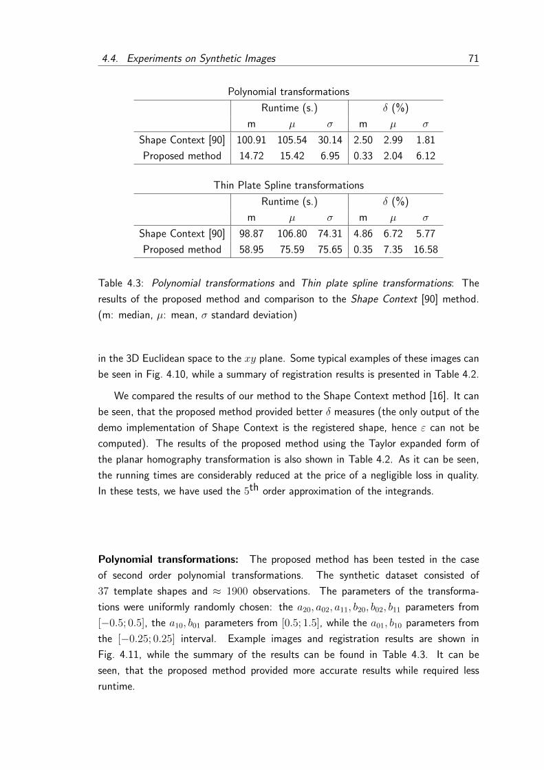
4.4. Experiments on Synthetic Images 71
Polynomial transformations
Runtime (s.) δ (%)
m µ σ m µ σ
Shape Context [90] 100.91 105.54 30.14 2.50 2.99 1.81
Proposed method 14.72 15.42 6.95 0.33 2.04 6.12
Thin Plate Spline transformations
Runtime (s.) δ (%)
m µ σ m µ σ
Shape Context [90] 98.87 106.80 74.31 4.86 6.72 5.77
Proposed method 58.95 75.59 75.65 0.35 7.35 16.58
Table 4.3: Polynomial transformations and Thin plate spline transformations: The
results of the proposed method and comparison to the Shape Context [90] method.
(m: median, µ: mean, σ standard deviation)
in the 3D Euclidean space to the xy plane. Some typical examples of these images can
be seen in Fig. 4.10, while a summary of registration results is presented in Table 4.2.
We compared the results of our method to the Shape Context method [16]. It can
be seen, that the proposed method provided better δ measures (the only output of the
demo implementation of Shape Context is the registered shape, hence ε can not be
computed). The results of the proposed method using the Taylor expanded form of
the planar homography transformation is also shown in Table 4.2. As it can be seen,
the running times are considerably reduced at the price of a negligible loss in quality.
In these tests, we have used the 5th order approximation of the integrands.
Polynomial transformations: The proposed method has been tested in the case
of second order polynomial transformations. The synthetic dataset consisted of
37 template shapes and ≈ 1900 observations. The parameters of the transforma-
tions were uniformly randomly chosen: the a20, a02, a11, b20, b02, b11 parameters from
[−0.5; 0.5], the a10, b01 parameters from [0.5; 1.5], while the a01, b10 parameters from
the [−0.25; 0.25] interval. Example images and registration results are shown in
Fig. 4.11, while the summary of the results can be found in Table 4.3. It can be
seen, that the proposed method provided more accurate results while required less
runtime.

72 Chapter 4. Nonlinear Registration of Binary Shapes
(a) missing pixels (b) occlusion (c) disocclusion (d) boundary error
Figure 4.12: Sample observations with various degradations for testing robustness.
Thin plate splines: For the synthetic test we used the the thin plate spline trans-
formation model with 5 control points placed in the following points:
(0, 0), (−0.25, − 0.25), (−0.25, 0.25), (0.25, − 0.25), (0.25, 0.25)
. The synthetic dataset was consisted of the 37 template shapes and their ≈ 1000 ob-
servations. The affine parts (the aij parameters) of the transformations were randomly
composed of 0.5, . . . , 1.5 scalings, −π4, . . . , π
4rotations, and −0.3, . . . , 0.3 shearing,
while the weights of the control points were chosen from −0.58, . . . , 0.58. Example
images and registration results are shown in Fig. 4.11, while the summary of the results
can be found in Table 4.3. It should be noted, that while the Shape Context placed
the control points on the boundaries of the objects, the proposed method used the
same 5 control point model with which the observation shapes were generated, which
is a non-negligible advantage.
Robustness: We examined the robustness of the proposed method against segmen-
tation errors on the synthetic dataset of planar homography. In the first testcase,
5%, . . . , 20% of the foreground pixels has been removed from the observations before
registration. In the second case, we occluded continuous square-shaped regions of size
equal to 1%, . . . , 10% of the shape, while in the third case we disoccluded a similar
region. Finally, we randomly added or removed squares uniformly around the boundary
of a total size 1%, . . . , 10% of the shape. Sample images can be found in Fig. 4.12.
The summary of the results can be found in Table 4.4. Results show that the
proposed method is quite robust in those cases where the segmentation errors are
uniformly distributed on the shapes (first and fourth testcases), and outperformed
the Shape Context method [16] in these cases. In those cases, however, when the
segmentation errors are consisted of larger continuous regions, like occlusion and dis-
occlusion, it provides less accurate results compared to the Shape Context. The reason
is that these large regions drastically change the value of the integrals in the system
of equations.

4.5. Experiments on Real Images 73
(a) missing pixels 5% 10% 15% 20%
Shape Context [16]m 21.85 24.91 26.38 27.2
σ 5.97 6.14 6.37 6.56
Proposed methodm 2.98 5.69 8.51 11.57
σ 4.13 5.23 6.09 6.74
(b) size of occlusion 1% 2.5% 5% 10%
Shape Context [16]m 3.03 3.55 4.55 6.79
σ 4.79 4.79 5.09 7.03
Proposed methodm 1.41 3.40 6.19 11.27
σ 3.49 4.18 5.09 6.6
(c) size of disocclusion 1% 2.5% 5% 10%
Shape Context [16]m 3.63 4.52 6.25 9.28
σ 5.19 5.61 6.84 7.78
Proposed methodm 1.93 4.54 8.28 13.62
σ 4.31 5.13 6.16 7.09
(d) size of boundary error 1% 5% 10% 20%
Shape Context [16]m 2.86 3.78 4.68 6.92
σ 4.72 4.83 5.04 5.92
Proposed methodm 0.54 1.67 2.67 4.03
σ 3.28 3.5 3.9 4.47
Table 4.4: Median (m) and standard deviation (σ) of δ error (%) vs. various type of
segmentation errors as shown in Fig. 4.12.
4.5 Experiments on Real Images
In this section we present the results of our algorithm in the case of various real
problems.
4.5.1 Planar Homography
Traffic signs: We tested the proposed method to register traffic signs. Nowadays,
many safety systems like radars and cameras are included in modern cars, thus one
possible application of the proposed method could be the pose-esimation of the signs.
In the case of a calibrated camera, the recovery of the exact spacial position of the sign
could be also possible, thus the system could alert the driver. While in the literature
there are automatic solutions for traffic sign detection and segmentation [82], we
used classical thresholding and some morphological operations to extract the shapes

74 Chapter 4. Nonlinear Registration of Binary Shapes
(a) (b) (c) (d) (e) (f)
Figure 4.13: Registration results on traffic signs. The first row shows the templates
while below them the corresponding observations with the overlaid contour of the
registration results.
from the images. Each template and observation image pair was taken from different
signboards. The main challenges were strong deformations, segmentation errors. In
addition, the style of the same object is also often vary between different signboards.
For example, the observations in Fig. 4.13(f), Fig. 4.15(b) and Fig. 4.15(c) do not
contain exactly the same shape as the object on the template. In particular, the STOP
sign in Fig. 4.15(c) uses different fonts. In spite of these difficulties, our method was
able to recover a quite accurate transformation. The average δ error was 12, 66% on
these images.
Medical X-ray images: Hip replacement is an important especially for elderly pa-
tients whose hip joint has been broken. In this surgical procedure the hip joint is
replaced by a prosthetic implant. After the operation inflammation often occurs, caus-
ing further loosening of fracture. In current practice, investigation of these loosenings
requires the inspection and comparison of X-ray images taken at different times af-
ter the operation. Automatic registration can help this visual inspection as clinically
significant prosthesis movement can be very small [33].
The registration is challenged by highly non-linear radiometric distortion which
makes the application of intensity-based methods difficult. On the other hand, the
segmentation of the implants is possible [79], we used active contours [18]. Another
problem is that the implant is positioned differently in 3D between the recording of
the X-ray images, leading to nonlinear transformation between the planar images.
Fortunately, these X-ray images are always taken in a well defined position of the
patient’s leg, the planar homography transformation can be assumed to be a good
approximation here. Some registration results can be found in Fig. 4.14.

4.5. Experiments on Real Images 75
SIFT [62] SC [16] Proposed
δ = 18.65% δ = 1.83% δ = 1.64%
δ = 2.84% δ = 10.23% δ = 1.32%
Figure 4.14: Registration results on hip prosthesis X-ray images. The overlaid contours
show the aligned contours of the corresponding images on the left. Images in the second
column show the registration results obtained by SIFT [62]+homest [60], in the third
column the results of Shape Context [16]+homest [60], while the last column contains
the results of the proposed method.
Comparison: We compared the results of our algorithm to the homest [60] soft-
ware which is also available online. Using different methods [117, 45], it estimates a
homography which minimizes a cost function obtained by point correspondences, and
filters out outliers using regression [86]. For point matching, the authors propose to
use the SIFT [61] method, which implements a scale and rotation invariant similarity
measure [62]. This method requires the grayscale version of the images as input, thus
we provided the masked signboard region for traffic sign matching and the prosthesis
region for medical registration. Furthermore, we also tested homest using the point

76 Chapter 4. Nonlinear Registration of Binary Shapes
(a) (b) (c) (d)
Figure 4.15: Registration results on traffic signs. The templates are in the first row,
then the results obtained by SIFT [62]+homest [60] (second row), where the images
show point correspondences between the images found by SIFT [62] in the third row.
The results obtained by Shape Context [16]+homest [60] (fourth row) and the proposed
method in the last row. The contours of the registered images are overlaid.

4.5. Experiments on Real Images 77
Figure 4.16: Sample images from the MNIST dataset and registration results using
a thin plate spline model. First and second rows show the images used as templates
and observations while the 3rd and 4th rows show the registration results obtained by
Shape Context [16] and the proposed method, respectively.
Runtime (sec.) δ (%)
m µ σ m µ σ
Shape Context [16] 35.02 34.43 7.58 7.86 9.40 4.71
Proposed method 10.00 9.81 1.47 7.66 8.93 4.22
Table 4.5: Comparative results on 2000 image pairs from the MNIST database. m, µ,
and σ stand for the median, mean, and standard deviation.
correspondences obtained by Shape Context, which required the binary shapes as input.
Although the SIFT parameter called distRatio, controlling the number of the
extracted correspondences, has been manually fine-tuned, we could not get reliable re-
sults due to the lack of rich radiometric features. Fig. 4.14 shows two results on X-ray
images while on traffic signs (see Fig. 4.15), SIFT could not find enough correspon-
dences in about half of the cases. As for Shape Context-based correspondences, we
got somewhat better alignments (an average δ of 33.47% for the traffic sign images).
4.5.2 Thin Plate Spline
Character matching: The proposed method has been applied for aligning hand-
written digits form the MNIST dataset. Aligning an observation to different templates
can be used to classify the shape; the lowest deformation gives the right class of the
questioned object [16]. Here we used 25 control points for the TPS model, these
control points were placed on the 5 × 5 regular grid over the input images, which
involves 2 · 25 + 6 = 56 model parameters. The equations were generated using the

78 Chapter 4. Nonlinear Registration of Binary Shapes
Figure 4.17: Registration results of printed signs. Top: planar templates. Bottom:
the corresponding observations with the overlaid contour of the registration results.
The first image pair shows the segmented regions used for registration. Note the typical
segmentation errors. (Images provided by ContiTech Fluid Automotive Hungaria Ltd.)
function set Eq. (4.41) with parameters 0 ≤ mi, ni ≤ 8, mi + ni ≤ 8 resulting in an
overdetermined system of 81 equations. During this test, image pairs of the same digit
has been aligned, it meant ≈ 2000 test cases. The images were of size 28× 28, some
example images and registration results can be found in Fig. 4.16. The results were
compared to the Shape Context [16] method, which also uses a thin plate spline model
but control points are placed on the contours of the shapes. Comparative results in
Table 4.5 show that our method provided slightly better results within 1/3 CPU time.
4.5.3 An Industrial Application
For easier installation, signs are printed on the surface of hoses used in car industry.
Complete signs are expected for admissible quality, thus these signs are visually in-
spected during manufacturing. We were developing an automatic inspection system,
in which the signs were compared to corresponding template shapes. In this process,
the proposed method was used for the shape alignment. The main challenges were
the segmentation errors and the complex distortions. The transformation model of the
printing procedure is as follows:
1. The stamp (basically a planar template of the sign) is positioned on the hose
surface. This can be described by a 2D rotation and scaling S : R2 → R2 of the
template.
2. Then the stamp is pressed onto the surface, modeled as a transformation γ :

4.6. Summary 79
R2 → R3 that maps the template’s plane to a cylinder with radius r:
γ(x) =[r sin
x1
r, x2,−r cos
x1
r
]T.
3. Finally, a picture is taken with a camera, which is described by a classical pro-
jective transformation P : R3 → R2 with an unknown camera matrix.
Thus the transformation
ϕ(x) = (P γ S)(x) (4.47)
acting between a planar template and its distorted observation has 11 parameters:
S has 3 parameters, γ has one (r), and P has 7 (six extrinsic parameters and the
focal length). Different ω sets has been tested in order to obtain the best aligments.
The function set in Eq. (4.42) provided the best results with parameters using all
combinations for αi ∈
0, π6, π
3
and (ni,mi) ∈ (1, 2), (2, 1), (1, 3), (3, 1) yielding a
system of 12 equations. The method has been tested on more than 150 image pairs
and it proved to be efficient in spite of segmentation errors and severe distortions.
4.6 Summary
In this chapter, a binary image registration method has been described. This general
framework can be applied to any diffeomorphic transformation model. Using only the
coordinates of the foreground pixels of the shapes, it sets up a system of equations and
the solution of this system provides the parameters of the aligning transformation. Thus
the approach does not require any feature detection and established correspondences.
The algorithm is easy to implement and experiments showed that it provides accurate
alignments. The robustness of the method against segmentation errors has also been
demonstrated, and it has been applied in the case of different real-world applications
where it clearly outperformed state-of-the-art correspondence based methods.


Chapter 5
Affine Invariants Based Projective
Registration of Binary Shapes
In the previous chapter, we described a robust method to estimate the parameters
of nonlinear transformations between binary shapes. The framework was sufficiently
applied to general nonlinear transformations, e.g., polynomial and thin plate spline,
and it been proved to be efficient in case of many real applications, e.g., matching
handwritten characters or aligning multimodal prostate images. Altough this approach
proved to be very robust against the strength of the deformation, in some cases (e.g.,
when the shapes are rotated more than 90 degrees), it can not find the right solution
due to the iterative minimization involved.
In this chapter another method is described to estimate the parameters of projective
transformations between binary shapes. The transformation is decomposed and the
perspective and the affine parts are recovered in two sequential steps. Similarly as
the method described in the previous chapter, it does not need any feature extraction
or established correspondences, it works only with the coordinates of the foreground
pixels.
5.1 The Registration Method
We are looking for the parameters of a two dimensional projective transformation (also
called planar homography) h : R2 → R2, h(x) = [h1(x), h2(x)]T that aligns the
input binary images, as it was described in Section 4.2.1. The parameters of such a
transformation are the Hij elements of the 3 × 3 matrix H, and H33 = 1 is fixed.
The template and the observation shapes are represented by their foreground regions
Ft ⊂ R2 and Fo ⊂ R2. Thus the correspondence between the two shapes can be
81

82 Chapter 5. Affine Invariants Based Projective Registration of Binary Shapes
written as
Ft = h(Fo). (5.1)
5.1.1 Decomposition of the Transformation
The H31 and H32 parameters of the transformation are responsible for the perspective
distortion, while the others generate an affine transformation (translation, rotation,
scaling and shearing). These two parts of the transformation can be performed one
after the other, so thus h can be decomposed as follows:
h = ha hp (5.2)
where hp : R2 → R2, hp(x) = [hp1(x), hp2(x)]T is a nonlinear transformation:
hp1(x) =x1
p1x1 + p2x2 + 1
hp2(x) =x2
p1x1 + p2x2 + 1, (5.3)
resulting only a perspective distortion. It has only two parameters p1 and p2. The
affine component ha : R2 → R2, ha(x) = [ha1(x), ha2(x)]T is a linear transformation
with 6 parameters:
ha1(x) = a11x1 + a12x2 + a13
ha2(x) = a21x1 + a22x2 + a23. (5.4)
The a13 and a23 parameters are responsible for translation, while scaling, shearing and
rotation are induced by the remaining four parameters.
Now we can write the relationship between the shapes as follows:
Ft = (ha hp)(Fo) = ha(hp(Fo)). (5.5)
The proposed method estimates the p1, p2 parameters of the perspective compo-
nent hp and the aij parameters of the affine component ha in two distinct steps, then
according to Eq. (5.2) we can obtain the Hij parameters of h as follows:
H11 = a11 + p1a13, H12 = a12 + p2a13,
H21 = a21 + p1a23, H22 = a22 + p2a23,
H13 = a13, H23 = a23, H31 = p1, H32 = p2 (5.6)
5.1. The Registration Method 83
5.1.2 Estimation of the Perspective Distortion
If Eq. (5.5) stands then there is only an affine transformation between Ft and hp(Fo),
thus for any affine-invariant function I : R2 → R:
I(Ft) = I(hp(Fo)). (5.7)
Note that the unknowns of this equation are the pi parameters of hp. Moreover as we
will show for given values of p1 and p2 using traditional moment-based affine invariants
the right hand side of the equation can be efficiently estimated using only the Jacobian
of hp, so it is not necessary to actually generate the image hp(Fo) which would be
very time-consuming.
The basic idea of the proposed method is that given a set of independent affine
invariant functions Ii : R2 → R, i = 1 . . . n we obtain a system of equations:
Ii(Ft) = Ii(hp(Fo)). (5.8)
The parameters of hp are obtained as the solution of this system of equations. It is
clearly a highly nonlinear system and thus do not have exact solution. However as
experimental results show it can be efficiently solved by a general nonlinear solver.
Although any set of affine invariant functions could be appropriate, herein we use
affine moment invariants [34], because it allows a very efficient numerical estimation
of the system of equations in Eq. (5.8). The left hand sides of the system of equations
Eq. (5.8) do not depend on the parameters of hp so can be estimated directly using
the point coordinates of the template image. The geometric moment mrs of order
(r + s) of a shape F is defined as
mrs(F) =
∫Fxr1x
s2dx. (5.9)
The affine moment invariants Ii of a shape are rely on the so called central moments
that are defined as follows:
µrs(F) =
∫F
(x1 − c1)r(x2 − c2)sdx (5.10)
where the coordinates of the center of mass of the shape are given by using the
geometric moments:
c1 =m10(F)
m00(F)and c2 =
m01(F)
m00(F). (5.11)
The affine moment invariants Ii(F ) then are obtained using these central moments.
For example the first two affine moment invariants are given as follows:
I1 = (µ20µ02 − µ211)/µ4
00
I2 = (−µ230µ
203 + 6µ30µ21µ12µ03 − 4µ30µ
312
−4µ321µ03 + 3µ2
21µ212)/µ10
00. (5.12)

84 Chapter 5. Affine Invariants Based Projective Registration of Binary Shapes
Algorithm 6: Pseudo code of the affine invariants based projective registration
methodInput : Binary images: template and observation
Output: The Hij parameters of the aligning planar homography
Choose a set of affine invariants Ii : R2 → R (i = 1, . . . , n)1
The solution of the system of equations Eq. (5.8) gives the perspective2
parameters p1 and p2
Solve the system of equations Eq. (5.17) to determine the affine parameters aij3
Use Eq. (5.6) to obtain the Hij parameters of the aligning planar homography4
For more on affine moment invariants see [34].
Given fixed parameters of hp we show how to compute the right hand side of the
equations Eq. (5.8) avoiding the generation of the image hp(Fo) by making use of the
Jacobian determinant |Jhp | of the transformation. For a shape F that is distorted by
hp the geometric moment can be estimated as follows:
mrs(hp(F)) =
∫F
[hp1(x)]r [hp2(x)]s |Jhp(x)|dx (5.13)
where the Jacobian of the perspective distortion is given by
|Jhp(x)| = 1
(p1x1 + p2x2 + 1)3, (5.14)
(for more details on the usage of the Jacobian and mathematical derivation of such
equations see Chapter 4 or [35]). On the perspectively distorted shape hp(F) the
central moments are given by
µrs(hp(F)) =
∫F
[hp1(x)− c1]r [hp2(x)− c2]s |Jhp(x)|dx, (5.15)
where
c1 =m10(hp(F))
m00(hp(F))and c2 =
m01(hp(F))
m00(hp(F)). (5.16)
For fixed values of the parameters p1 and p2 the affine moment invariants I(hp(F ))
in the right hand side of the system Eq. (5.8) can be obtained using the central moments
in Eq. (5.15) that can be estimated using only the foreground points of the shape F .
Thus we avoid to generate the hp(F) images which would be very time consuming.
5.1.3 Estimation of the Affine Component
After the p1 and p2 parameters of the perspective distortion are estimated, the affine
transformation ha should be recovered between the shapes Ft and hp(Fo). For that

5.2. Implementational Issues 85
Template Observation Step 1 Step 2
Figure 5.1: The registration process: The first step removes only the perspective distor-
tion from the observation image while the second step restores the affine transformation
and thus align it to the original template image.
purpose we used the approach proposed in [30]. In order to avoid the generation of
hp(Fo) we modified the method by making use of the Jacobian |Jhp | of the perspective
component. The following system of equations
∫Ft
ynkdy = |Jha |n∑i=1
(n
i
) i∑j=0
(i
j
)an−ik1 ai−jk2 a
jk3
∫Fo
hp1(x)n−ihp2(x)i−j|Jhp(x)|dx,
(5.17)
for n = 1, 2, 3 and k = 1, 2 can be written for the aij parameters of the affine
transformation. This system contains six polynomial equations up to order three which
is enough to solve for all the 6 unknowns.
The Jacobian of an affine transformation is constant over the whole plane, and it
equals to the ratio of the areas of the shapes:
|Jha | =∫Ft dy∫
Fo |Jhp(x)|dx(5.18)
Although the system of equations in Eq. (5.17) may have many solutions, we
can select that real root which corresponds to the determinant what we computed in
Eq. (5.18). Note that the solution is not unique if the shape is affine symmetric.
Putting together the projective transformation hp and the affine transformation
ha using Eq. (5.6) we get the Hij parameters of the aligning planar homography
transformation h.
5.2 Implementational Issues
Although the two unknowns of the perspective part hp would require only a system of
two equations, i.e., two invariants in system Eq. (5.8), the independence of the chosen
set of affine moment invariants is not guaranteed. Accordingly we found that using
overdetermined system of equations the method provides more accurate alignments.

86 Chapter 5. Affine Invariants Based Projective Registration of Binary Shapes
δ(%) ε (pixel)
m µ σ m µ σ
Shape Context 10.10 13.36 11.02 - - -
Parametric 10.54 14.31 13.99 151.60 122.72 87.21
AMI Based 2.38 6.23 12.34 1.88 23.46 53.00
Table 5.1: Test results on the synthetic dataset of Shape Context, the parametric
framework (Chapter 4) and the AMI based method. m, µ, and σ denote the median,
mean, and deviation.
The results shown in Section 5.3 was obtained using the I3, I4, I5, I6 set of invari-
ants. While the system is clearly nonlinear we found that it could be solved efficiently
using nonlinear optimization methods, and in our experiments, we used the standard
differential evolution [99] method. The equations are constructed in the continuum but
in practice we only have a limited precision digital image. Consequently, the integrals
over the continuous domains Ft and Fo can only be approximated by discrete sums
over the set of foreground pixel. The pseudo code of the proposed algorithm can be
found in Algorithm 6 while Fig. 5.1 shows example registration results after the two
subsequent steps of the method.
5.3 Experiments
We examined the performance of the proposed method on a large synthetic dataset
consist of 35 different template shapes and their projectively distorted versions as
observations a total of ≈ 1100 images of size 300 × 300. The applied projective
transformations were randomly composed of 0.5, . . . , 1.5 scalings; −π4, . . . , π
4rotations
along the x and y axes and −π, . . . , π along the z axe; −1, . . . , 1 translations along
both x and y axis and 0.5, . . . , 2.5 along the z axis; and a random focal length chosen
from the [0.5, 1.5] interval.
Registration results were quantitatively evaluated using the two kind of error mea-
sures defined in Eq. (4.40). The summary of the results is shown in Table 5.1.
For comparison we examined the results of the parametric framework described
in Chapter 4 on the same dataset. It provided weaker results since could not cope
with cases when the images were rotated more than 90 degrees. We have also com-
pared the performance of our method to that of Shape Context [16], a more general
shape matching algorithm developed for nonlinear registration of binary images. For
our experiments, we used the program provided by the authors, its parameters were
set empirically to their optimal value (beta init = 30 , n iter = 30 , annealing rate

5.4. Discussion 87
Template Observation Shape Context Parametric AMI based
Figure 5.2: Example images from the synthetic data set and registration results ob-
tained by Shape Context [16], the parametric framework (Chapter 4) and the AMI
based method. The template and the registered observation were overlaid, overlap-
ping pixels are depicted in gray whereas nonoverlapping ones are shown in black.
r = 1 ). The average running time of the parametric and the AMI based method (C
implementations) were 4.75 sec. and 12.86 sec. respectively. The runtime of the
Matlab implementation of Shape Context (68.87 sec.) is not authoritative. We also
tested the proposed method on traffic signs. Some registration results can be found
in Fig. 5.3
5.4 Discussion
In our experiments, we found that in its current form, the algorithm is not robust
enough against segmentation errors. On the one hand, this is due to that the applied
affine moment invariants are based on high-order geometrical moments, and these
statistics are sensitive to small shape changes. On the other hand, when the first
step could not estimate accurately the p1 and p2 parameters, and thus the perspective
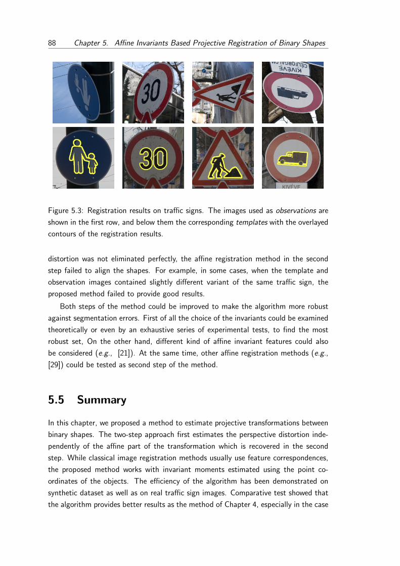
88 Chapter 5. Affine Invariants Based Projective Registration of Binary Shapes
Figure 5.3: Registration results on traffic signs. The images used as observations are
shown in the first row, and below them the corresponding templates with the overlayed
contours of the registration results.
distortion was not eliminated perfectly, the affine registration method in the second
step failed to align the shapes. For example, in some cases, when the template and
observation images contained slightly different variant of the same traffic sign, the
proposed method failed to provide good results.
Both steps of the method could be improved to make the algorithm more robust
against segmentation errors. First of all the choice of the invariants could be examined
theoretically or even by an exhaustive series of experimental tests, to find the most
robust set, On the other hand, different kind of affine invariant features could also
be considered (e.g., [21]). At the same time, other affine registration methods (e.g.,
[29]) could be tested as second step of the method.
5.5 Summary
In this chapter, we proposed a method to estimate projective transformations between
binary shapes. The two-step approach first estimates the perspective distortion inde-
pendently of the affine part of the transformation which is recovered in the second
step. While classical image registration methods usually use feature correspondences,
the proposed method works with invariant moments estimated using the point co-
ordinates of the objects. The efficiency of the algorithm has been demonstrated on
synthetic dataset as well as on real traffic sign images. Comparative test showed that
the algorithm provides better results as the method of Chapter 4, especially in the case

5.5. Summary 89
of strong deformations, e.g., when the shapes are rotated more than 90 degrees. The
method in its described form is sensitive to segmentation errors, however this can be
improved in the future work.


Appendix A
Summary in English
Binary shapes play important role in the field of image processing, due to that
1. the images of many real world objects are basically binary shapes, e.g., text
characters, traffic signs, bones or implants on X-ray images, etc.
2. in most of the image processing applications at some point of the processing
pipeline the images are binarized (i.e., segmented).
In many cases, the additional information that we are working with a binary valued
image limits the number of possible solutions (the search space) thus it can help to
obtain more accurate results. For example, the linear inverse problems like tomography
and deconvolution are usually under-determined, and have many possible solutions.
Knowing that we are seeking a binary image restricts the search space, and as a result,
for example in the case of tomography, binary images can be usually reconstructed
accurately only from a few projections.
In many other cases, however, the lack of rich intensity information makes it difficult
to deal with these binary images. For example image registration techniques commonly
work with previously established point pairs and these correspondences are usually
obtained using the intensity patterns around points. Thus in the case of binary images
these methods can not obtain appropriate point correspondences. On the other hand,
in the case of binary images we do not need to deal with the intensity change between
the images. Therefore many techniques has been presented previously to register binary
images using statistics computed using the point coordinates of the shapes.
Chapter 2 addresses the problem of discrete tomography. In this field, it is com-
monly assumed that the intensity values of the images (i.e., the attenuation coefficients
of the materials) are a priori accurately known. In practice, however, this information is
usually not available and hard to determine. The author proposes novel reconstruction
method for those cases, when the intensity values are unknown. Using higher order
91

92 Appendix A. Summary in English
statistics based discretization term, the solution automatically converges to binary sets.
Comparative tests showed, that the proposed method is more robust to the projection
noise as a state-of-the-art algorithm. The method has also been successfully applied
on real data.
In Chapter 3, a binary tomography based image deblurring method is introduced.
Tikhonov regularization based 1-dimensional deconvolution is proposed to restore the
horizontal and vertical projections. In this approach, the L-curve method is used to
determine the regularization parameter which provides the best trade-off between the
norm of the residual (data-fit term) and the norm of the solution (smoothness). To
reconstruct the shapes from the restored projections, a maximum-flow based binary
tomography method is applied. Comparative synthetic tests show that the method
can provide reliable result even in the case of low signal-to-noise ratio images, thanks
to that the L-curve method can provide a good regularization parameter for any noise
level. Results on real out-of-focus images are also presented.
In Chapter 4, the nonlinear registration of binary images is addressed. A general
framework is proposed to estimate the parameters of a diffeomorphism that aligns
two binary shapes. The framework is applied to different widely-used transformation
classes. Comparisons to other state-of-the-art methods are conducted and the robust-
ness to different type of segmentation errors is examined. The algorithm has also been
successfully applied in different real-world applications.
Chapter 5 introduce a technique to estimate the parameters of a planar homog-
raphy transformation between binary shapes. In this method the planar homography
is decomposed into the perspective distortion and the affine transformation and the
parameters of these two parts are estimated separately in two consecutive steps. Com-
parative synthetic tests and results on real images are presented.
Summary of the Thesis Points
In the followings the list of the key points of the dissertation is given. Table A shows
the connection between the thesis points and the publications of the author. The
planar homography related results of the thesis point III. was also previously presented
in [77].
I.) The author introduces a novel higher order statistics based binary tomography
reconstruction technique, which can be used in those cases, when the inten-
sity values of the images are unknown. He proposes an objective functional in
which a discretization term is applied to prescribe binary solutions. He propose
to minimize the objective functional by a graduated non-convexity optimization

93
approach, in which the weight of the discretization term is increased during the
optimization process to gradually enforce binary solutions. He proposes to esti-
mate the mid-level of the intensities directly to the intermediate solutions in each
iteration step. This mid-level is estimated as the minimum of the discretization
term. The author examines the convergence properties of the method and shows
that the behaviour of the method is independent of the value of the intensities.
He demonstrates the robustness of the algorithm against different strengths of
projection noise. The author compares his algorithm to state-of-the-art methods
and shows that his approach is a good alternative. He also successfully applies
his algorithm to real projection data.
II.) The author proposes a binary tomography based approach for the deconvolution
of binary images. He proposes to deconvolve the projections of the blurred images
using a Tikhonov regularization based approach, in which the optimal value of
the regularization parameter is found by the L-curve method. To reconstruct the
shapes from their deblurred projections, he applies a maximum-flow based binary
tomography method. He shows in comparative tests that his method provides
more reliable results then another widely-used method. He also presents results
on real out-of-focus images.
III.) The author addresses the problem of nonlinear registration of binary shapes. A
general registration framework is used which traces back the registration prob-
lem to a system of nonlinear equations. He applies the framework to different
nonlinear transformation classes such as planar homography, polynomial trans-
formations, and thin plate splines. He goes into the implementational details
and shows that the equations can be written in three alternative forms which
improves the registration results. In the case of planar homography, the author
shows that the performance of the algorithm can be improved if we apply it to the
Taylor series expansion of the transformation. The author proposes different ω
function sets to construct the system of equations and compares them. He pro-
poses to normalize the equations to guarantee equal contribution to the objective
functional. The author compares the method to other state-of-the-art methods
on synthetic datasets, and examines the robustness of the algorithm against dif-
ferent types of segmentation errors. The author shows that the method can be
applied in different real world applications.
IV.) The author proposes an affine moment invariants based approach to estimate
the parameters of a planar homography transformation between binary shapes.
He shows how to decompose the transformation into a perspective and an affine
part and recover their parameters separately in two consecutive steps. He shows

94 Appendix A. Summary in English
how to estimate the projective parameters of the transformation using affine
moment invariants. As a second step, he applies an affine registration method to
determine the remaining parameters of the transformation. The author compares
the method to the algorithm presented in the previous thesis point and shows
results obtained by the algorithm on real images.
[73] [74] [76] [75] [32] [72]
I. •II. •III. • • •IV. •
Table A.1: Correspondence between the thesis points and the publications.

Appendix B
Summary in Hungarian
A binaris kepek fontos szerepet jatszanak a kepfeldolgozas teruleten, mivel
1. sok objektum kepe alapjaban veve binaris, peldaul karakterek, KRESZ tablak,
csontok vagy implantatumok a rontgenkepeken, stb,
2. a kepfeldolgozo rendszerek tobbsegeben a feldolgozas bizonyos pontjan a kepeket
binarizaljak, azaz szegmentaljak.
Sok esetben az a tobbletinformacio, hogy a kep, amivel dolgozunk csak ket in-
tenzitaserteket tartalmaz, leszukıti a keresesi teret, azaz a lehetseges megoldasok hal-
mazat, ezert segıt, hogy pontosabb eredmenyekhez jussunk. Peldaul a linearis inverz
problemak (mint peldaul a tomografia vagy a dekonvolucio) sokszor aluldefinialtak
es tobb lehetseges megoldasuk van. Tudva, hogy egy binaris kepet keresunk,
leszukıthetjuk a keresesi teret. Ennek koszonhetoen peldaul a tomografia eseteben
a binaris kepek sokszor nehany vetuletbol is pontosan rekonstrualhatoak.
Mas esetekben azonban az intenzitasertekek valtozatossaganak hianya megnehezıti
a binaris kepekkel valo munkat. Peldaul a kepregisztracios modszerek gyakran korabban
kinyert pontmegfeleltetesekbol dolgoznak es ezek a megfeleltetesek altalaban a pon-
tok koruli intenzitas mintazatok alapjan tortennek. Ezert binaris kepeken ezek a
modszerek nem tudnak megfelelo pontmegfelelteteseket kinyerni. Masreszrol binaris
kepek eseten nem kell foglalkoznunk a kepek kozotti intenzitas-valtozassal. Ezert sok
olyan modszert fejlesztettek ki, melyek a binaris alakzatok regisztraciojahoz a pontko-
ordinatakbol szamıtott statisztikakat hasznaljak.
A 2. fejezetben diszkret tomografiaval foglalkozunk. Ezen a teruleten gyakran
feltetelezik, hogy a rekonstrualando kepeken levo intenzitasertekek (s ıgy az anyagok
elnyelodesi egyutthatoi) apriori ismertek. A gyakorlatban azonban ez az informacio
altalaban nem all rendelkezesre es nehez meghatarozni. Egy uj rekonstrukcios modszert
mutatunk be azokra az esetekre, amikor az intenzitas szintek ismeretlenek. Magasabb
95

96 Appendix B. Summary in Hungarian
foku statisztika alapu diszkretizacios fuggveny segıtsegevel a megoldas automatikusan
binarizalodik. Osszehasonlıto tesztek megmutattak, hogy a bemutatott modszer ro-
bosztusabb a vetuleti zajjal szemben mint egy masik, korszeru modszer. A modszer
valos adatokon elert eredmenyei is bemutatasra kerultek.
A 3. fejezetben binaris tomografia alapu kepelesıto modszert mutatunk be.
Egy Tikhonov-regularizacio alapu 1-dimenzios dekonvolucios eljarassal helyreallıtjuk
a kep fuggoleges es vızszintes vetuleteket. L-curve modszert hasznalunk a
megfelelo regularizacios parameter meghatarozasahoz. Az alakzatoknak a helyreallıtott
vetuleteikbol valo rekonstrukciojahoz, egy maximalis folyam alapu binaris tomografiai
modszert hasznalunk. Osszehasonlıto tesztek mutatjak, hogy a modszer megbızhato
eredmenyeket nyujt meg alacsony jel-zaj aranyu kepeken is, koszonhetoen annak, hogy
az L-curve modszer megfelelo regularizacios parametert ad magas zajszintek eseten is.
Valos eletlen kepeken elert eredmenyeket is bemutatunk.
A 4. fejezet binaris kepek nemlinearis regisztraciojaval foglalkozik. Egy
altalanos keretrendszert mutatunk be, mely binaris kepek kozotti diffeomorfiz-
musok parametereinek meghatarozasara hasznalhato. A keretrendszert kulonbozo
szeleskorben hasznalt transzformacios modell eseteben is alkalmazzuk. Szintetikus
tesztek megmutattak, hogy a modzser robosztus kulonbozo szegmentalasi hibakkal
szemben. Az algoritmust sikeresen alkalmaztuk kulonbozo valos problemak eseten.
A 5. fejezet binaris kepek kozott sıkhomografia parametereinek meghatarozasara
mutat be modszert. A sıkhomografia transzformaciot felbontjuk egy perspektıv es
egy affin transzformaciora es ezek parametereit kulon-kulon hatarozzuk meg ket
egymasutani lepesben. Osszehasonlıto tesztek eredmenyeit es valos kepeken elert
eredmenyeket is bemutatunk
Az eredmenyek tezisszeru osszefoglalasa
A kovetkezokben felsoroljuk a szerzo eredmenyeit tezispontokba foglalva. A Table B.
tablazat mutatja, hogy a szerzo publikacioi mely tezispontokhoz kapcsolodnak. A III.
tezispont sıkhomografiara vonatkozo eredmenyei a [77] munkaban is be lettek mutatva.
I.) A szerzo kidolgozott egy uj, magasab foku statisztikat hasznalo binaris to-
mografiai technikat, amely azokban az esetekben is alkalmazato, amikor a kepek
intenzitasertekei ismeretlenek. Egy olyan celfuggvenyt javasol, amelyben egy dis-
zkretizacios tag ırja elo a binaris megoldasokat. A celfuggveny minimalizalasahoz
egy fokozatos optimalizalasi strategiat mutat be, amelyben a diszkretizacios tag
sulya novekszik, ıgy fokozatosan kenyszerıti ki a binaris megoldasokat. Az in-
teniztasertekek kozepszintjenek becslese a diszkretizacios tag minimalizalasaval

97
tortenik. A szerzo megvizsgalta a modszer konvergencia-tulajdonsagait es meg-
mutatja hogy az algoritmus viselkedese fuggetlen az intenzitasertekektol. Bemu-
tatja a modszer robosztussagat a kulonbozo merteku vetuleti zajokkal szemben.
A modszert osszehasonlıtotta mas korszeru modszerekkel es megmutatta, hogy
az algoritmusa jo alternatıvat jelent. Sikeresen hasznalta a modszert valos ada-
tokon.
II.) A szerzo egy binaris tomografia alapu binaris kephelyreallıtasi modszert mutat
be. Az elmosodott kepek vetuleteit Tikhonov regularizacio segıtsegevel allıtja
helyre. A megfelelo regularizacios parameter kivalasztasahoz az L-curve modszert
javasolja. A helyreallıtott vetuletekbol egy maximum-folyam-alapu binaris to-
mografiai modszerrel rekonstrualja az alakzatot. Osszehasonlıto teszt mutatja,
hogy a modszer sok esetben jobb eredmenyeket er el mint egy masik, szeleskorben
hasznalt modszer. A szerzo bemutat valos kameraval keszıtett, elmosodott
kepeken elert eredmenyeket is.
III.) A szerzo binaris alakzatok nemlinearis regisztraciojaval foglalkozik. Egy altalanos
regisztracios keretrendszert hasznal, amely a regisztracios problemat egy egyen-
letrendszer megoldasara vezeti vissza. A keretrendszert kulonbozo nemlinearis
transzformacios osztalyok eseteben is alkalmazza, mint peldaul sıkhomografia,
polinomialis transzformaciok es thin-plate-spline transzformacio. Bemutatja
az implementacios reszleteket es azt, hogy az egyenletek oda-vissza torteno
felırasaval hogyan lehet javıtani a modszer eredmenyein. A sıkhomografia
eseteben megmutatja, hogy az algoritmus hatekonysaga javıthato, ha a transz-
formacio Taylor sorba fejtett valtozatan alkalmazzuk a keretrendszert. Kulonbozo
ω fuggveny halmazokat vizsgal az egyenletrendszer felırasahoz, es osszehasonlıtja
oket. A szerzo az egyenletek normalizalasaval eri el, hogy azok azonos modon
jaruljanak hozza a celfuggvenyhez. A szerzo osszehasonlıtja a modszert mas
korszeru technikakkal szintetikus adatokon es megvizsgalja a javasolt algoritmus
robosztussagat a szegmentalasi hibakkal szemben. A szerzo bemutatja a modszer
eredmenyeit tobb valos problema eseten, mint peldaul rontgenkepek vagy KRESZ
tablak illesztese.
IV.) A szerzo egy affin momentum invariansokon alapulo modszert mutat be binaris
alakzatok kozotti sıkhomografia transzformacio parametereinek becslesere. Meg-
mutatja, hogyan lehet felbontani a transzformaciot egy perspektıv es egy af-
fin osszetevore. A parameterek meghatarozasa ket, egymast koveto lepesben
tortenik. Az elso lepes csak a perspektıv torzulast allıtja helyre a megfigyelt
kepen, mıg a masodik lepes meghatarozza az affin transzformaciot ıgy megkapjuk

98 Appendix B. Summary in Hungarian
az eredeti sablon kepet. A szerzo osszehasonlıtja modszert az elozo pontban be-
mutatott technikaval es bemutat valos kepeken elert eredmenyeket is.
[73] [74] [76] [75] [32] [72]
I. •II. •III. • • •IV. •
Table B.1: A tezispontok es a szerzo publikacioinak kapcsolata.

Bibliography
[1] A. M. Bruckstein A. M. Bronstein, M. M. Bronstein and R. Kimmel. Analysis
of two-dimensional non-rigid shapes. International Journal of Computer Vision,
78:67–88, June 2008.
[2] Anubhav Agarwal, C. V. Jawahar, and P. J. Narayanan. A survey of planar
homography estimation techniques. Technical report, International Institute of
Informatics Technology, Hyderabad 500019 India, June 2005.
[3] A.H. Andersen and A.C. Kak. Simultaneous algebraic reconstruction technique
(SART): A superior implementation of the ART algorithm. Ultrasonic Imaging,
6(1):81–94, January 1984.
[4] Marton Balasko, Attila Kuba, Antal Nagy, Zoltan Kiss, Lajos Rodek, and Laszlo
Rusko. Neutron-, gamma- and x-ray three-dimensional computed tomography
at the budapest research reactor site. Nuclear Instruments and Methods in
Physics Research Section A: Accelerators, Spectrometers, Detectors and Associ-
ated Equipment, 542(1–3):22–27, 2005. Proceedings of the Fifth International
Topical Meeting on Neutron Radiography ITMNR-5 Fifth International Topical
Meeting on Neutron Radiography.
[5] Marton Balasko, Attila Kuba, Attila Tanacs, Zoltan Kiss, Antal Nagy, and
Burkhard Schillinger. Comparison radiography and tomography possibilities of
FRM-II (20 mw) and Budapest (10 MW) Research Reactor. In Muhammed
Arif, editor, Proceedings of the Eight World Conference WCNR-8, pages 18–27,
October 2008.
[6] Peter Balazs and Mihaly Gara. An evolutionary approach for object-based image
reconstruction using learnt priors. In Proceedings of the 16th Scandinavian Con-
ference on Image Analysis, pages 520–529. Springer-Verlag Berlin, Heidelberg,
2009.
99

100 Bibliography
[7] JohnathanM. Bardsley and John Goldes. Regularization parameter selection and
an efficient algorithm for total variation-regularized positron emission tomogra-
phy. Numerical Algorithms, 57(2):255–271, 2011.
[8] K. J. Batenburg. An evolutionary algorithm for discrete tomography. Discrete
Applied Mathematics, 151:36–54, October 2005.
[9] K. J. Batenburg. A network flow algorithm for reconstructing binary images from
continuous x-rays. Journal of Mathematical Imaging and Vision, 30(3):231–248,
2008.
[10] K. J. Batenburg, W. Van Aarle, and J. Sijbers. A semi-automatic algorithm for
grey level estimation in tomography. Pattern Recognition Letters, 32:1395–1405,
July 2011.
[11] K. J. Batenburg and J. Sijbers. Optimal threshold selection for tomogram seg-
mentation by projection distance minimization. IEEE Transactions on Medical
Imaging, 28:676–686, 2009.
[12] K. J. Batenburg and J. Sijbers. DART: A practical reconstruction algorithm for
discrete tomography. IEEE Transactions on Image Processing, 20(9):2542–2553,
2011.
[13] K. J. Batenburg, J. Sijbers, H.F. Poulsen, and E. Knudsen. DART: A robust
algorithm for fast reconstruction of 3D grain maps. Journal of Applied Crystal-
lography, 43:1464–1473, 2010.
[14] Kees J. Batenburg, Marta D. Rossell, Rolf Erni, Gustaaf Van Tendeloo, and
Sandra Van Aert. Three-dimensional atomic imaging of crystalline nanoparticles.
Nature, 470:374–377, 2011.
[15] Kees Joost Batenburg. A network flow algorithm for reconstructing binary images
from discrete x-rays. Journal of Mathematical Imaging and Vision, 27(2):175–
191, 2007.
[16] Serge Belongie, Jitendra Malik, and Jan Puzicha. Shape matching and object
recognition using shape context. Transaction on Pattern Analysis and Machine
Intelligence, 24(4):509–522, April 2002.
[17] A. Blake and A. Zisserman. Visual Reconstruction. Artificial Intelligence. MIT
Press, 2003.

Bibliography 101
[18] Thomas Boudier. The snake plugin for ImageJ. software http://www.snv.
jussieu.fr/~wboudier/softs/snake.html.
[19] S. Brunetti, A. Del Lungo, F. Del Ristoro, A. Kuba, and M Nivat. Reconstruction
of 4- and 8-connected convex discrete sets from row and column projections.
Linear Algebra and its Applications, 339(1–3):37–57, December 2001.
[20] S. Brunetti, P. Dulio, and C. Peri. Discrete tomography determination
of bounded lattice sets from four x-rays. Discrete Applied Mathematics,
161(15):2281 – 2292, 2013.
[21] Darshan Bryner, Anuj Srivastava, and Eric Klassen. Affine-invariant, elastic
shape analysis of planar contours. In IEEE Proceedings of Conference on Com-
puter Vision and Pattern Recognition, pages 390–397, June 2012.
[22] James A. Cadzow. Blind deconvolution via cumulant extrema. IEEE Signal
Processing Magazine, 13:24–42, May 1996.
[23] T.D. Capricelli and P.L. Combettes. A convex programming algorithm for noisy
discrete tomography. In Gabor T. Herman and Attila Kuba, editors, Advances
in Discrete Tomography and Its Applications, Applied and Numerical Harmonic
Analysis, pages 207–226. Birkhauser Boston, 2007.
[24] Thomas Capricelli. Convex processing. software http://labs.freehackers.
org/projects/cvx-processing.
[25] Yair Censor. Binary steering in discrete tomography reconstruction with sequen-
tial and simultaneous iterative algorithms. Linear Algebra and its Applications,
339:111–124, December 2001.
[26] Marek Chorbak and Christoph Durr. Reconstructing hv-convex polyominoes from
orthogonal projections. Information Processing Letters, 69:283–289, 1999.
[27] M. Holden D. L. G. Hill, P. G. Batchelor and D. J. Hawkes. Medical image
registration. Physics in Medicine and Biology, 46:R1–R45, March 2001.
[28] S. R. Deans. The Radon transform and some of its applications. A Wiley-
Interscience publication. Wiley, 1983.
[29] Csaba Domokos and Zoltan Kato. Binary image registration using covariant
gaussian densities. In Aurelio Campilho and Mohamed Kamel, editors, Proceed-
ings of International Conference on Image Analysis and Recognition, volume
5112 of Lecture Notes in Computer Science, pages 455–464, Povoa de Varzim,
Portugal, June 2008. Springer.

102 Bibliography
[30] Csaba Domokos and Zoltan Kato. Parametric estimation of affine deformations
of planar shapes. Pattern Recognition, 43:569–578, March 2010.
[31] Csaba Domokos, Zoltan Kato, and Joseph M. Francos. Parametric estimation
of affine deformations of binary images. In Proceedings of the International
Conference on Acoustics, Speech, and Signal Processing, pages 889–892, Las
Vegas, Nevada, USA, April 2008.
[32] Csaba Domokos, Jozsef Nemeth, and Zoltan Kato. Nonlinear shape registration
without correspondences. IEEE Transactions on Pattern Analysis and Machine
Intelligence, 34(5):943–958, May 2012.
[33] M.R. Downing, P.E. Undrill, P. Ashcroft, D.W.L. Hukins, and J.D. Hutchison.
Automated femoral measurement in total hip replacement radiographs. In Pro-
ceedings of International Conference on Image Processing and Its Applications,
volume 2, pages 843–847, Dublin, Ireland, July 1997. IEEE.
[34] Jan Flusser, Tomas Suk, and Barbara Zitova. Moments and Moment Invariants
in Pattern Recognition. Wiley & Sons, October 2009.
[35] J.M. Francos, R. Hagege, and B. Friedlander. Estimation of multidimensional
homeomorphisms for object recognition in noisy environments. In Proceedings
of Conference on Signals, Systems and Computers, volume 2, pages 1615–1619,
Pacific Grove, California, USA, November 2003.
[36] R.J. Gardner, P. Gritzmann, and D. Prangenberg. On the computational com-
plexity of reconstructing lattice sets from their x-rays. Discrete Mathematics,
202(1–3):45–71, 1999.
[37] Vito Di Gesu, Giosue Lo Bosco, Filippo Millonz, and Cesare Valenti. A memetic
algorithm for binary image reconstruction. In ValentinE. Brimkov, RenetaP.
Barneva, and HerbertA. Hauptman, editors, Combinatorial Image Analysis, vol-
ume 4958 of Lecture Notes in Computer Science, pages 384–395. Springer Berlin
Heidelberg, 2008.
[38] Ardeshir Goshtasby. Registration of images with geometric distortions. IEEE
Tran. on Geoscience and Remote Sensing, 26(1):60–64, January 1988.
[39] J. Gregor and T. Benson. Computational analysis and improvement of SIRT.
IEEE Transactions on Medical Imaging, 27(7):918–924, 2008.
[40] H. Guo, A. Rangarajan, S. Joshi, and L. Younes. Non-rigid registration of shapes
via diffeomorphic point matching. In Proceedings of International Symposium on

Bibliography 103
Biomedical Imaging: From Nano to Macro, volume 1, pages 924–927, Arlington,
VA, USA, April 2004. IEEE.
[41] T. Tuytelaars H. Bay, A. Ess and L. Van Gool. Speeded-up robust features
(SURF). Computer Vision and Image Understanding, 110:346–359, August 2008.
[42] D. Groisser H. D. Tagare and O. Skrinjar. Symmetric non-rigid registration:
A geometric theory and some numerical techniques. Journal of Mathematical
Imaging and Vision, 34:61–88, May 2009.
[43] Lajos Hajdu. Unique reconstruction of bounded sets in discrete tomography.
Electronic Notes in Discrete Mathematics, 20:15 – 25, 2005.
[44] Per Christian Hansen and Dianne P. O’Leary. The use of the L-curve in the regu-
larization of discrete ill-posed problems. SIAM Journal on Scientific Computing,
14:1487–1503, 1993.
[45] Richard Hartley. In defense of the eight-point algorithm. IEEE Transactions on
Pattern Analysis and Machine Intelligence, 19(6):580–593, June 1997.
[46] Gabor T. Herman and Attila Kuba, editors. Discrete Tomography: Foundations,
Algorithms, and Applications. Birkhauser Boston, 1999.
[47] Gabor T. Herman and Attila Kuba, editors. Advances in Discrete Tomography
and its Applications. Birkhauser Boston, 2007.
[48] G.T. Herman. Fundamentals of Computerized Tomography: Image Reconstruc-
tion from Projections. Advances in Pattern Recognition. Springer London, 2009.
[49] A. C. Kak and M. Slaney. Principles of Computerized Tomographic Imaging.
IEEE Press, 1988.
[50] S. Kaneko, Y. Satohb, and S. Igarashi. Using selective correlation coefficient for
robust image registration. Pattern Recognition, 36:1165–1173, May 2003.
[51] Jeongtae Kim and Soohyun Jang. High order statistics based blind deconvolution
of bi-level images with unknown intensity values. Optics Express, 18(12):12872–
12889, June 2010.
[52] C. Kisielowski, P. Schwander, F.H. Baumann, M. Seibt, Y. Kim, and A. Our-
mazd. An approach to quantitative high-resolution transmission electron mi-
croscopy of crystalline materials. Ultramicroscopy, 58(2):131–155, 1995.

104 Bibliography
[53] Attila Kuba and Murice Nivat. A sufficient condition for non-uniqueness in binary
tomography with absorption. Theoretical Computer Science, 346(2–3):335–357,
2005. In memoriam: Alberto Del Lungo (1965-2003).
[54] M. Pawan Kumar, Sujit Kuthirummal, C. V. Jawahar, and P. J. Narayanan.
Planar homography from fourier domain representation. In Proceedings of In-
ternational Conference on Signal Processing and Communications, 2004.
[55] Edmund Y. Lam. Blind bi-level image restoration with iterated quadratic pro-
gramming. IEEE Transactions on Circuits and Systems Part 2: Express Briefs,
54(1):52–56, 2007.
[56] Edmund Y. Lam and Joseph W. Goodman. Iterative statistical approach to blind
image deconvolution. Journal of the Optical Society of America A, 17(7):1177–
1184, 2000.
[57] Silvio Levy. Projective transformations. web page, http://www.geom.uiuc.
edu/docs/reference/CRC-formulas/node16.html.
[58] Ta-Hsin Li. A joint estimation approach for two-tone image deblurring by blind
deconvolution. IEEE Transactions on Image Processing, 11:847–858, August
2002.
[59] Ta-Hsin Li and Ke-Shin Lii. Deblurring two-tone images by a joint estimation
approach using higher-order statistics. In Proceedings of IEEE SP Workshop on
Higher-Order Statistics, pages 108–111, 1997.
[60] Manolis Lourakis. homest: A C/C++ library for robust, non-linear homogra-
phy estimation. software, http://www.ics.forth.gr/~lourakis/homest/,
2008.
[61] David Lowe. Demo software: SIFT keypoint detector. software, http://www.
cs.ubc.ca/~lowe/keypoints/, July 2005.
[62] David G. Lowe. Distinctive image features from scale-invariant keypoints. Inter-
national Journal of Computer Vision, 60(2):91–110, November 2004.
[63] Tibor Lukic. Discrete tomography reconstruction based on the multi-well poten-
tial. Proceedings of the 14th International Confereence on Combinatorial Image
Analysis, 6636:335–345, 2011.
[64] J. B. Antoine Maintz and Max A. Viergever. A survey of medical image regis-
tration. Medical Image Analysis, 2(1):1–36, March 1998.

Bibliography 105
[65] Steve Mann and Rosalind W. Picard. Video orbits of the projective group a
simple approach to featureless estimation of parameters. IEEE Transactions on
Image Processing, 6(9):1281–1295, September 1997.
[66] Donald W. Marquardt. An algorithm for least-squares estimation of nonlinear
parameters. SIAM Journal on Applied Mathematics, 11(2):431–441, 1963.
[67] S. Marsland and C. J. Twining. Constructing diffeomorphic representations for
the groupwise analysis of nonrigid registrations of medical images. IEEE Trans-
actions on Medical Imaging, 23:1006–1020, August 2004.
[68] E.V. Moisi, B. Nagy, and V.I. Cretu. Maximum flow minimum cost algorithm
for reconstruction of images represented on the triangular grid. In IEEE 8th
International Symposium on Applied Computational Intelligence and Informatics,
pages 35–40, May 2013.
[69] Abris Nagy and Csaba Vincze. Reconstruction of hv-convex sets by their coordi-
nate x-ray functions. Journal of Mathematical Imaging and Vision, 49(3):569–
582, 2014.
[70] Antal Nagy. Smoothing filters in the dart algorithm. In RenetaP. Barneva,
ValentinE. Brimkov, and Josef L lapal, editors, Combinatorial Image Analysis,
volume 8466 of Lecture Notes in Computer Science, pages 224–237. Springer
International Publishing, 2014.
[71] Antal Nagy and Attila Kuba. Reconstruction of binary matrices from fan-beam
projections. Acta Cybernetica, 17(2):359–385, January 2005.
[72] Jozsef Nemeth. Recovering projective transformations between binary shapes. In
Proceedings of Advanced Concepts for Intelligent Vision Systems, volume 7517,
pages 374–383, Brno, Czech Republic, 2012.
[73] Jozsef Nemeth. Discrete tomography with unknown intensity levels using higher-
order statistics. Journal of Mathematical Imaging and Vision, 2015. Online first,
DOI: 10.1007/s10851-015-0581-0.
[74] Jozsef Nemeth and Peter Balazs. Restoration of blurred binary images using
discrete tomography. In Proceedings of Advanced Concepts for Intelligent Vision
Systems, volume 8192, pages 80–90, Poznan, Poland, 2013.
[75] Jozsef Nemeth, Csaba Domokos, and Zoltan Kato. Nonlinear registration of
binary shapes. In Proceedings of International Conference on Image Processing,
pages 1101–1104, Cairo, Egypt, November 2009. IEEE.

106 Bibliography
[76] Jozsef Nemeth, Csaba Domokos, and Zoltan Kato. Recovering planar homo-
graphies between 2D shapes. In Proceedings of International Conference on
Computer Vision, pages 2170–2176, Kyoto, Japan, September 2009. IEEE.
[77] Jozsef Nemeth. Sıkhomografia parametereinek becslese binaris kepeken. In
Proceedings of National Scientific Students’ Associations Conference, April 2009.
Supervisors: Zoltan Kato and Csaba Domokos. Note: in Hungarian.
[78] Jorge Nocedal and Stephen J. Wright. Numerical optimization. Springer series
in operations research and financial engineering. Springer, New York, NY, 2. ed.
edition, 2006.
[79] Alina Oprea and Constantin Vertan. A quantitative evaluation of the hip pros-
thesis segmentation quality in x-ray images. In Proceedings of International
Symposium on Signals, Circuits and Systems, volume 1, pages 1–4, Iasi, Roma-
nia, July 2007. IEEE.
[80] James B. Orlin. A polynomial time primal network simplex algorithm for mini-
mum cost flows. In Proceedings of the Seventh Annual ACM-SIAM Symposium
on Discrete Algorithms, SODA ’96, pages 474–481, Philadelphia, PA, USA,
1996. SIAM.
[81] N. Otsu. A threshold selection method from gray-level histograms. IEEE Trans-
actions on Systems, Man and Cybernetics, 9(1):62–66, January 1979.
[82] Carlos Filipe Paulo and Paulo Lobato Correia. Automatic detection and clas-
sification of traffic signs. In Proceedings of Workshop on Image Analysis for
Multimedia Interactive Services, pages 11–14, Santorini, Greece, June 2007.
[83] Marc Pollefeys. Scene planes and homographies. Presentation, www.cs.unc.
edu/~marc/mvg/course16.ppt.
[84] William Hadley Richardson. Bayesian-based iterative method of image restora-
tion. Journal of the Optical Society of America, 62(1):55–59, Jan 1972.
[85] A. Rosenfeld and A.C. Kak. Digital Picture Processing. 2.ed. Number v. 1-2.
Academic Press, 1982.
[86] Peter J. Rousseeuw. Least median of squares regression. Journal of the American
Statistics Association, 79(388):871–880, December 1984.
[87] Stephane Roux, Hugo Leclerc, and Francois Hild. Efficient binary tomographic
reconstruction. Journal of Mathematical Imaging and Vision, 49(2):335–351,
2014.

Bibliography 107
[88] H.J. Ryser. Combinatorial properties of matrices of zeros and ones. In Classic Pa-
pers in Combinatorics, Modern Birkhauser Classics, pages 269–275. Birkhauser
Boston, 1987.
[89] J. Malik S. Belongie and J. Puzicha. Shape context demo soft-
ware. http://www.eecs.berkeley.edu/Research/Projects/CS/vision/
shape/sc\_digits.html, 2002.
[90] J. Malik S. Belongie and J. Puzicha. Shape matching and object recognition
using shape context. IEEE Transactions on Pattern Analysis and Machine Intel-
ligence, 24(4):509–522, April 2002.
[91] Robert J. Schalkoff. Digital Image Processing and Computer Vision. John Wiley
& Sons, New York, NY, USA, 1989.
[92] T. Schule, C. Schnorr, S. Weber, and J. Hornegger. Discrete tomography by
convex–concave regularization and D.C. programming. Discrete Applied Math-
ematics, 151:229–243, October 2005.
[93] Thomas Schule, Stefan Weber, and Christoph Schnorr. Adaptive reconstruction
of discrete-valued objects from few projections. Electronic Notes in Discrete
Mathematics, 20:365–384, July 2005.
[94] Behzad Sharif and Behnam Sharif. Discrete tomography in discrete deconvolu-
tion: Deconvolution of binary images using ryser’s algorithm. Electronic Notes
in Discrete Mathematics, 20:555–571, July 2005.
[95] Yijiang Shen, Edmund Y. Lam, and Ngai Wong. Binary image restoration by
positive semidefinite programming. Optics Letters, 32(2):121–123, 2007.
[96] K. M. Simonson, S. M. Drescher, and F. R. Tanner. A statistics-based approach
to binary image registration with uncertainty analysis. IEEE Transactions on
Pattern Analysis and Machine Intelligence, 29:112–125, January 2007.
[97] Katherine M. Simonson, Steven M. Drescher, and Franklin R. Tanner. A
statistics-based approach to binary image registration with uncertainty analysis.
IEEE Transactions on Pattern Analysis and Machine Intelligence, 29:112–125,
January 2007.
[98] A. Singer and H. Wu. Two-dimensional tomography from noisy projections taken
at unknown random directions. SIAM Journal on Imaging Sciences, 6(1):136–
175, 2013.

108 Bibliography
[99] Rainer Storn and Kenneth Price. Differential evolution - a simple and efficient
heuristic for global optimization over continuous spaces. Journal of Global Op-
timization, 11(4):341–359, December 1997.
[100] Tomas Suk and Jan Flusser. Affine normalization of symmetric objects. In
Jacques Blanc-Talon, Wilfried Philips, Dan Popescu, and Paul Scheunders, edi-
tors, Proceedings of International Conference on Advanced Concepts for Intelli-
gent Vision Systems, volume 3708 of Lecture Notes in Computer Science, pages
100–107, Antwerp, Belgium, September 2005. Springer.
[101] A.N. Tikhonov and V.I.A. Arsenin. Solutions of ill-posed problems. Scripta series
in mathematics. Winston, 1977.
[102] Jeannot Trampert and Jean-Jacques Leveque. Simultaneous iterative reconstruc-
tion technique: Physical interpretation based on the generalized least squares
solution. Journal of Geophysical Research, 95(B8):12553–12559, August 1990.
[103] Cesare Valenti. A genetic algorithm for discrete tomography reconstruction. Gen.
Progr. Evolv. Mach., 9(1):85–96, March 2008.
[104] Wim van Aarle, Kees Joost Batenburg, and Jan Sijbers. Automatic parameter
estimation for the discrete algebraic reconstruction technique (DART). IEEE
Transactions on Image Processing, 21(11):4608–4621, 2012.
[105] Wim van Aarle, Karel Crombecq, Ivo Couckuyt, K. Joost Batenburg, and Jan
Sijbers. Efficient parameter estimation for discrete tomography using adaptive
modelling. In Fully Three-Dimensional Image Reconstruction in Radiology and
Nuclear Medicine, pages 229–232, July 2011.
[106] Laszlo Varga, Peter Balazs, and Antal Nagy. Projection selection algorithms for
discrete tomography. In J. Blanc-Talon, D. Bone, W. Philips, D. Popescu, and
P. Scheunders, editors, Proceedings of the Advanced Concepts for Intelligent
Vision Systems, volume 6474 of Lecture Notes in Computer Science, pages 390–
401, Sydney, Australia, December 2010.
[107] Laszlo Varga, Peter Balazs, and Antal Nagy. Direction-dependency of binary to-
mographic reconstruction algorithms. Graphical Models, 73:365–375, November
2011.
[108] Laszlo Varga, Peter Balazs, and Antal Nagy. An energy minimization reconstruc-
tion algorithm for multivalued discrete tomography. In Proceedings of the 3rd
International Symposium on Computational Modeling of Objects Represented in
Images, pages 179–185, Rome, Italy, September 2012. Taylor & Francis.

Bibliography 109
[109] J. A. Ventura and W. Wan. Accurate matching of two-dimensional shapes using
the minimal tolerance zone error. Image and Vision Computing, 15:889–899,
December 1997.
[110] M.N. Vrahatis, G.S. Androulakis, J.N. Lambrinos, and G.D. Magoulas. A class of
gradient unconstrained minimization algorithms with adaptive stepsize. Journal
of Computational and Applied Mathematics, 114(2):367 – 386, 2000.
[111] Stefan Weber. Discrete tomography by convex–concave regularization using
linear and quadratic optimization. PhD thesis, Heidelberg University, 2009.
[112] Norbert Wiener. Extrapolation, Interpolation, and Smoothing of Stationary Time
Series with Engineering Applications. John Wiley & Sons, New York, NY, USA,
1949.
[113] Ralph A Wiggins. Minimum entropy deconvolution. Geoexploration, 16(1–2):21–
35, 1978.
[114] S. Worz and K. Rohr. Physics-based elastic registration using non-radial basis
functions and including landmark localization uncertainties. Computer Vision
Image Understanding, 111(3):263–274, September 2008.
[115] H.S. Wu. Minimum entropy deconvolution for restoration of blurred two-tone
images. Electronic Letters, 26:1183–1184, July 1990.
[116] A. Yezzi, L. Zollei, and T. Kapurz. A variational framework for joint segmentation
and registration. In Proceedings of IEEE Workshop on Mathematical Methods
in Biomedical Image Analysis, pages 44–51, Kauai, HI, USA, December 2001.
IEEE.
[117] O. Faugeras Z. Zhang, R. Deriche and Q. T. Luong. A robust technique for
matching two uncalibrated images through the recovery of the unknown epipolar
geometry. Artificial Intelligence, 78(1-2):87–119, October 1995.
[118] L. Zagorchev and A. Goshtasby. A comparative study of transformation functions
for nonrigid image registration. IEEE Transactions on Image Processing, 15:529–
538, March 2006.
[119] Barbara Zitova and Jan Flusser. Image registration methods: A survey. Image
and Vision Computing, 21(11):977–1000, October 2003.


![Mat 140.geometric shapes[1]](https://static.fdocuments.in/doc/165x107/5469a9b8af7959cb768b4c9a/mat-140geometric-shapes1.jpg)