GEOMETRIC AND MATERIAL NONLINEAR EFFECTS IN ELASTIC-PLASTIC AND FAILURE ANALYSES OF ANISOTROPIC

LAMINATED STRUCTURES

by

Dave Rourk

Dissertation submitted to the Faculty of the Virginia Polytechnic Institute and State University

in partial fulfillment of the requirements

D. Frederick

T. K~amy

for the degree of

Doctor of Philosophy

in

Engineering Mechanics

APPROVED:

j. N. Reddy ,G:ha i rman

December, 1986 Blacksburg, Virginia

E. G. Henneke, II

A. C. Loos

GEOMETRIC AND MATERIAL NONLINEAR EFFECTS IN ELASTIC-PLASTIC AND FAILURE ANALYSES OF ANISOTROPIC

LAMINATED STRUCTURES

by

Dave Rourk Department of Engineering Science and Mechanics

Virginia Polytechnic Institute and State University

(ABSTRACT)

In this study, an analytical procedure to predict the strength and

failure of laminated composite structures under monotonically increasing

static loads is presented. A degenerated 3-D shell finite element that

includes linear elastic and plastic material behavior with full

geometric nonlinearity is used to determine stresses at selected points

(Gauss quadrature points in each element) of the structure. Material

stiffness (constitutive) matrices are evaluated at each Gauss point, in

each lamina and in each element, and when the computed stress state

violates a user selected failure criterion, the material stiffness

matrix at the failed Gauss point is reduced. The reduction procedure

involves setting the material stiffnesses to unity. Examples of

isotropic, orthotropic, anisotropic and composite laminates are

presented to illustrate the validity of the procedure developed and to

evaluate various failure theories. Maximum stress, modified Hills

{Mathers}, Tsai-Wu (F12 = 0), and Hashin's failure criteria are

included.

The results indicate that for large length-to-thickness ratios, the

geometric nonlinear effect should be incorporated for both isotropic and

anisotropic structures. The nonlinear material model influences the

behavior of isotropic structures with small length-to-thickness ratios,

while having nearly no effect at all on laminated anisotropic

structures. Of the four failure theories compared, each predicts

failure at nearly the same load levels and locations. Hashin's

criterion is particularly noteworthy in that the mode fs also predicted.

Acknowledgements

The author would like to express his heartfelt thanks to Professors

Reddy, Frederick, Henneke, Kuppusamy and Loos for their encouragement

and support throughout this project.

The monetary support of this research by the Mechanics Division of

the Office of Naval Research and the Mathematical Sciences Section of

the Army Research Office is gratefully acknowledged.

To the courage to go beyond where you thought you could go,

and especially to those who inspire that courage within each

of us.

iv

CHAPTER 1.

CHAPTER 2.

TABLE OF CONTENTS

Page INTRODUCTION............................................ 1 1.1 Preliminary Comments •••••.••.....•..••••••••••.•... 1.2 Objective of the Present Study •.••.••••••••••.••.•. 1.3 Background Literature .•...................•........

GOVERNING EQUATIONS ...•.•..•.•.•...........•.•••........ 2.1 Incremental Form of the Equilibrium Equations •.•.•. 2.2 Finite Element Geometry and Formulation •••••••••... 2.3 Material Nonlinearity ••••••....•••.•••••••••••••.•. 2.4 Computational Procedure •••.•...•••.•••••••••••••••. 2.5 Assumptions and Procedures Used in the Program •••.• 2.6 Reducing Stress States to the Plasticity Functions

1 3 4

18 18 21 30 37 40

Surface............................................ 42

CHAPTER 3. NUMERICAL RESULTS •.•.••••.•••..•......•..••••••••.•••... 46 3.1 Isotropic Thick Plate •••..•.........••.•••••••.•... 46 3.2 Orthotropic and Cross Ply Thin Plate ••.••••••.•.•.. 48 3.3 Isotropic Cylindrical Shell .........•••••••••.•.•.. 48 3.4 Isotropic Spherical Shell ••........••••••••••.•••.. 48 3.5 Combined Geometric and Material Nonlinearities •••.. 51 3.6 Plate Strip .•.•••••••••••.••....•.•••••••••••••••.. 55

3.6.l Isotropic Plate Strip •..•••.•••••••••••••••. 55 3.6.2 Orthotropic Plate Strip •••...••••••••••.•... 57 3.6.3 Cross-Ply Plate Strip ...•••..••••••••••.•.•. 64 3.6.4 Angle Ply (45°/-45°) Plate Strip •••••••.•••. 66

CHAPTER 4. SUMMARY AND DISCUSSION •••••••.••••..•.•..•••••••••••••.• 70 4.1 General Comments .....•....•..............•••....... 70 4.2 Geometric and Material Nonlinear Effects •••.•.•••.• 71 4.3 Failure Criteria .•••.•..•.................•....•... 71 4.4 Recommendations ..•.•.•..•................••........ 72

CHAPTER 5. References. • . • . . . . • • . • • • • • • • • • • • . . .. . • . . .. . . • . . • • • • . • • . . . . 7 4

Appendix A: Material Properties Used in this Study ..••.•••••.•.•... 80

Vita................................................................ 83

v

CHAPTER 1

INTRODUCTION

1.1 Preliminary Comments

The ability to predict the behavior of a laminated, composite

structure beyond the first-ply failure is important in the preliminary

and final design of structures. Also, the prediction of how the

strength of a structure decreases under applied loads can be of great

help to designers and engineers.

Today, it is routine to do most structural analyses using the

finite element method. By far, the elements most frequently used in

common structural problems are based on plate or shell theories. To

keep up with the recent developments in the use of composite materials,

these elements have been modified to include the variation of stresses

and strains through the thickness of the laminate. The plate and shell

theories are two-dimensional approximations of the 3-0 elasticity

theory, and these theories do not account for the changes in geometry

during deformation. Three-dimensional elements based on the 3-0

elasticity theory become impractical to use in laminated structures

because at least one element would be required to model each lamina of a

laminate, and then, keeping within a reasonable aspect ratio of element

length to thickness, many elements would be required to model any

laminate.

A compromise between the elements based on plate or shell theory

and the three-dimensional elements in modelling a laminate is a

degenerated three-dimensional (3-0) shell or plate element. The 3-0

1

2

degenerated element is based on the three-dimensional elasticity

equations with three assumptions; 1) a line straight and normal to the

middle surface before deformaton remains straight, but not necessarily

normal to the middle surface, after deformation, 2) the strain energy

from the stresses perpendicular to the middle surface are ignored, and

3) the shell thickness-to-curvature ratio is small. The first

assumption allows the modeling of shear deformation, important in thick

shells. The second assumption improves the numerical conditioning of

the element since these strain energies are generally small compared to

the others, and the third assumption implies that derivatives at either

end of a middle surface normal line of the shell with respect to the

shell coordinates are the same. Therefore, the Jacobian matrix is free

of the through-the-thickness coordinate and numerical integration need

only be performed in the surface of the shell.

With the stress-strain information in hand, the problem of defining

how the material fails requires a criterion based on physical

considerations. There have been many failure criteria proposed for

anisotropic materials, and a review is presented in Section 1.3. If a

set of failure criteria were at hand, and a classification of material

systems to failure criteria existed, then the designer or engineer could

simply choose the particular failure criterion that went with the

material system the structure was to be made from. While this

classification doesn't exist per se, an intelligent choice of several

failure criteria can be made from knowing some basic information about

the material system used.

3

1.2 Objective of the Present Study

The overall objective of the present study is to develop a

computational procedure to predict failure in laminated anisotropic

structures composed of orthotropic laminae, and to determine the

strength reduction due to an applied static load. In the interest of

utilizing the high strength and stiffness of composite materials the

stress states within these materials will be pushed to higher levels

causing plastic material behavior in addition to possible geometric non-

1 inearities.

Three major tasks are to be completed in order to achieve the

objective:

1. The 3-0 degenerated element must be extended to include

material non-linearity in composite laminates. This will be

done using an associated flow rule with isotropic work

hardening (that is, the hardening will be incorporated into the

yield function by equating plastic work done in different

stress directions). This is the mechanism that will reduce

stiffnesses at plastically stressed points in the structure.

2. The failure criteria must be incorporated into the

computational scheme. Since the loading will be iterative, a

given failaure criterion must be checked at each Gauss point,

and at each load level, for each element. This will signal

where in the structure the lamina properties are to be reduced.

3. A comparison of the failure predictions of several failure

criteria when applied to an anisotropic structure undergoing

geometric and material nonlinear behavior will be undertaken.

4

After these steps are completed, an analytical method for

predicting where, and in what mode (shear, tensile, compressive),

failure will occur in a composite structure will be available.

1.3 Background Literature

The application of the finite element method to the analysis of

laminated composite shells, including geometric and material

nonlinearities is relatively a recent occurrence (see (1-10]). The

composite laminates are treated as an equivalent single layer [3] or as

a degenerated 3-D continuum [1,2]. The geometric nonlinearity used in

single-layer theories is one of the van Karman type, whereas the full

nonlinearity is used in the degenerated 3-D theories. The material

nonlinearity has been approached from either the micromechanics or

macromechanics points of view.

Micromechanics Models

In the micromechanics approach, the matrix is considered as an

elastic-plastic material while the fibers are considered to be brittle-

elastic. An elastic-plastic continuum model for fiber reinforced

composites was developed by Mulhern, Rogers and Spencer (11]. In this

model the composite material is treated as transversely isotropic, with

inextensible fibers and a rigid-perfectly plastic matrix. The yield

surface was formulated in terms of invariants characteristic of the

transversely isotropic geometry. The extension of an elastic fiber with

an elastic-perfectly plastic coating was considered by Mulhern et al.

(12]. The stages of development of the plastic zone in the fiber

coating was examined. These were compared to the results obtained by

5

Hill [13]. Hill 1 s solution differed in that the fiber coating yielded

instantaneously. The two solutions essentially agreed. In a later

publication [14], Mulhern et al. extended their earlier continuum theory

[11] to include an elastic fiber and an elastic-perfectly plastic

matrix. The assumed yield function was unaffected by normal stress in

the fiber direction, this eliminated the prediction of hysteresis loops

found in their earlier work [12]. Spencer [15] extended this theory to

a composite reinforced by two families of fibers. This was useful in

studying the behavior of composite laminates. The same model was used

in other applications, such as the dynamic analysis of composite beams

[16] and large deformation of composite structures [17,18].

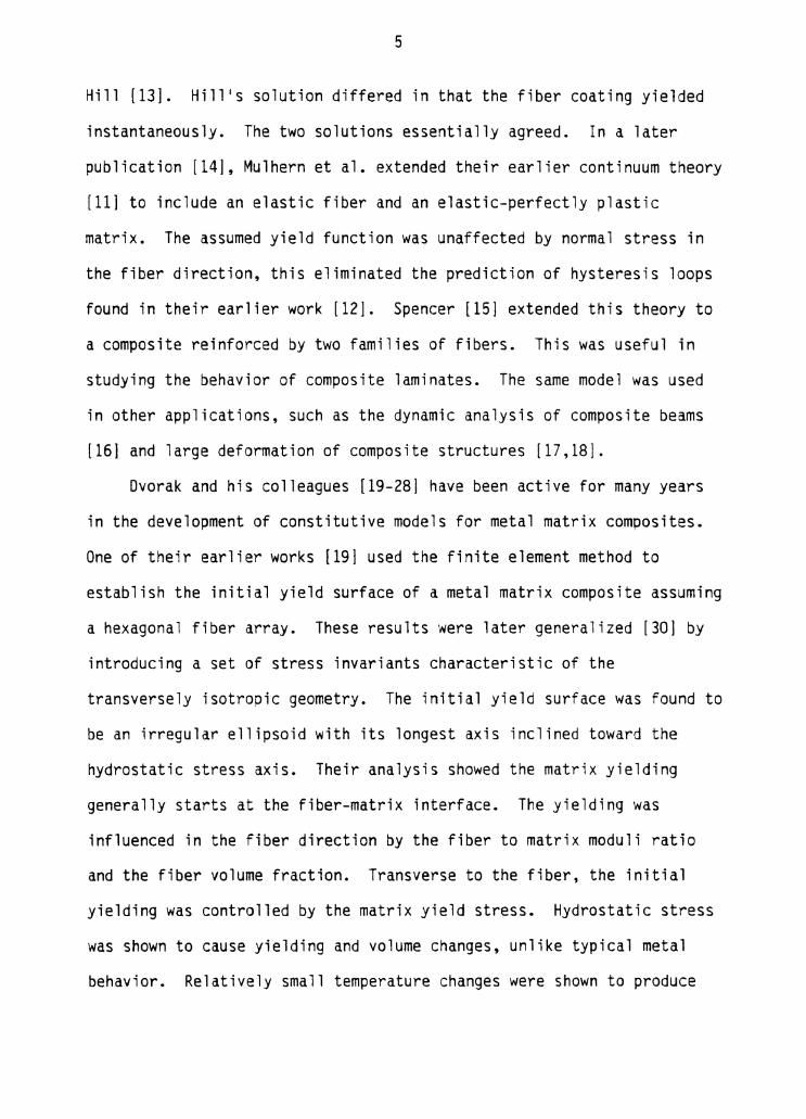
Dvorak and his colleagues [19-28] have been active for many years

in the development of constitutive models for metal matrix composites.

One of their earlier works [19] used the finite element method to

establish the initial yield surface of a metal matrix composite assuming

a hexagonal fiber array. These results were later generalized [30] by

introducing a set of stress invariants characteristic of the

transversely isotropic geometry. The initial yield surface was found to

be an irregular ellipsoid with its longest axis inclined toward the

hydrostatic stress axis. Their analysis showed the matrix yielding

generally starts at the fiber-matrix interface. The yielding was

influenced in the fiber direction by the fiber to matrix moduli ratio

and the fiber volume fraction. Transverse to the fiber, the initial

yielding was controlled by the matrix yield stress. Hydrostatic stress

was shown to cause yielding and volume changes, unlike typical metal

behavior. Relatively small temperature changes were shown to produce

6

matrix yielding. Values as small as 70° F were shown to cause initial

yielding for a boron/aluminum composite with a 10,000 psi matrix yield

stress. Based upon their investigation of initial yield surfaces,

Dvorak and Rao (21] developed a simple but accurate continuum plasticity

theory for axisymmetric deformation of unidirectional fibrous

composites. Assuming elastic fibers with a nonhardening matrix, a

simple hardening rule and associated flow rule was formulated. In

comparison with a composite cylinder model evaluated by the finite

element method for a complex load history, the continuum theory showed

very good agreement. Their axisymmetric theory, also applied to the

problem of analyzing uniform temperature changes in a metal matrix

composite, showed considerable success [22].

The elastic-plastic behavior of fibrous composites was explored by

Dvorak and Bahei-El-Din (23] using the self-consistent micromechanics

scheme [13]. The authors modified the scheme to alleviate the problems

reported by Huchinson [29], who observed high estimates of initial yield

stress and low plastic strains in the early stages of deformation. To

correct this problem, the authors replaced the elastic inclusion by a

composite cylinder model of Dvorak and Rao [21]. For the case of

axisymmetric mechanical loading, the modified self-consistent model

produced similar results to the unmodified self-consistent model and the

composite cylinder model. The authors examined the case of initial

yield due to longitudinal shear loading, the modified self-consistent

model performed well while the unmodified self-consistent model

encountered some difficulties. Calculations of longitudinal shear loads

gave an initial yield stress which was substantially higher than the

7

matrix yield stress. This contradicts initial yield estimates obtained

by the finite element analysis [20], which showed the initial yield

stress well below the matrix yield stress. The modifications to the

self-consistent model were found to improve the performance, yet they

were found to be prohibitively difficult for nonsymmetric loading.

In order to obtain a general constitutive model and retain

computational simplicity, Dvorak and Bahei-El-Din [24,30] introduced a

simple micromechanics model which they called the Vanishing Fiber

Diameter Model. In this model it was assumed that each of the

cylindrical fibers have a vanishing diameter while the fiber volume

fraction in the composite remains finite. In effect the fiber imposes a

constraint on the matrix in the longitudinal direction. The simplicity

of this model allows for the easy incorporation of any matrix material

nonlinearity. This was demonstrated by Lou and Schapery [31] in which a

nonlinear viscoelastic material model was used in conjunction with a

similar model. Bahei-El-Din [25-30] incorporated the Vanishing Fiber

Diameter model with a Mises-type matrix material which obeys the Prager-

Ziegler kinematic hardening rule. This constitutive model was used in

classical lamination theory and a three-dimensional finite element

analysis code called PAC78. In order to obtain good correlation with

experimental results, Bahei-El-Din resorted to using in-situ matrix

properties, since the unreinforced matrix properties yielded poor

results. Initial yield surfaces computed for a cross-ply laminate

showed reasonable agreement compared to results obtained by a finite

element computation from Rao [32]. Experimental results for a

cyclically loaded laminate were compared to the results from PAC78

8

[28]. The predicted strains in the load direction showed very good

agreement. The strains in the unloaded direction were over-estimated.

The authors suggest the discrepancy could be a result of neglecting the

fiber-matrix constraint in the transverse direction.

Hoffman [33] developed a plane stress initial yield criterion for

metal matrix composites based upon the concept of partial stresses. The

partial stress concept is based on the stress in the laminate satisfying

equilibrium and compatibility. The equilibrium condition is that the

total stress is equal to the sum of the matrix and the fiber stresses,

and the compatibility condition requires that the strains in the matrix

and the fiber are identical. Retaining only the axial fiber stiffness,

Hoffman then obtained a very simple expression for the Mises 1 yield

condition in terms of the matrix stresses. Min [34], using Hoffman 1 s

partial stress model, developed an elastic-plastic material model which

incorporated a kinematic hardening rule similar to that of Bahei-El-Din

and Dvorak [27] for a nonhardening matrix material. Min and Crossman

[35] used a plane stress mechanics of materials model for the

elastoplastic deformation analysis of unidirectional composites

subjected to both thermal and mechanical loading. The model explicitly

accounts for the microstresses and the thermal residual stresses but

only for a nonhardening matrix. The model of Min and Crossman was

extended by Min and Flaggs [36,37] by adding a White-Besseling

plasticity model [38] for the matrix material. The resulting

constitutive model was incorporated into a nonlinear laminate analysis

program. The nonlinear system of equations obtained in the laminate

analysis was solved by a modified Newton method with a line search

9

[39]. The thermal cycling-induced deformations of a unidirectionally

reinforced graphite/magnesium composite were examined by Wolf, Min and

Kural [40), who used the mechanics of material model developed by Min

and Flagg [36,37) to analyze the complex thermal load history. The

comparison was poor. Explanations for the behavior were attributed to

the temperature dependence of the matrix yield stress (which was ignored

in the analysis) and the presence of matrix creep.

Ruffin, Rimbos and Bigelow [41) developed an elastic-plastic point

stress laminate analysis program called MLAP. Their program was

formulated using the Vanishing Fiber Diameter model and a kinematic

hardening Mises-type matrix material based upon Dvorak and Bahei-El-Din

[25,28]. Comparison of experimental results and predictions by MLAP

showed fair agreement. Program MLAP over-predicted the transverse

strains, which seems to be characteristic of the micromechanics

formulation [28]. The authors used unreinforced matrix material

properties; possibly their results could have been improved by using in-

situ properties like Dvorak and Bahei-El-Din [28).

Aboudi, in a series of papers [42-45), developed a continuum model

for fiber reinforced elastic-viscoplastic composites. The theory is

formulated for a viscoplastic matrix with transversely isotropic or

viscoplastic fiber. The unidirectional fibers were assumed to have

rectangular cross sections and were arranged in a doubly periodic

rectangular array. This geometry allowed the use of Legendre

polynomials for the expansion of the displacement field within each sub-

cel l. The solution was obtained by imposing displacement and stress

continuity at the sub-cell interfaces and appropriate boundary

10

conditions on the unit cell. The author obtained a first order solution

to his general theory and demonstrated excellent agreement for the

elastic case with other micromechanics solutions. Comparisons with

experimental results also showed good agreement. The transverse and

shear moduli results were particularly promising. No viscoplastic

computations were compared with experimental results. This would have

made it possible to assess the relative performance of Aboudi's model to

the Vanishing Fiber Diameter model of Dvorak. Several examples of the

viscoplastic behavior were compared to available finite element

solutions, and good agreement was demonstrated.

Macromechanics Models

One of the first attempts at analyzing the nonlinear behavior of

composites at the macromechanics level was performed by Petit and

Waddoups [46]. The authors considered the nonlinearities uncoupled in

the longitudinal, transverse and shear directions which acted

independently during combined loading. Failure of individual plies were

determined by a maximum strain criterion. The authors made certain

assumptions upon the behavior of the failed plies. Transverse ply

failure implied that load could still be carried in the longitudinal or

shear directions. Similarly, shear failure implied that load could

still be carried in the longitudinal or transverse directions.

Longitudinal failure, however, implied a total ply failure and no

further load carrying capability. The authors incorporated these

principles into a laminate analysis program. The plies were allowed

successive failures until the laminate ultimately failed. The

11

correlation to experimental results for stress-strain response was fair

to good, but the failure predictions were generally poor.

Hahn and Tsai [47] modeled nonlinear shear response of a composite

by introducing a complementary elastic energy density function. A

polynomial expansion of the complementary elastic energy density

function was performed. In addition to the second order terms which

describe the linear elastic behavior, one fourth-order term was retained

to describe the nonlinear shear behavior. The application of this model

to unidirectional (see Hahn and Tsai [47]) and multidirectional

composite systems (see Hahn [48]) produced fair results.

The anisotropic plasticity theory of Hill [49,50,32] has inspired

many subsequent researchers to develop constitutive models. Hill

originally proposed his theory to model the weakly orthotropic behavior

typically found in cold rolled metals. In this theory it is assumed

that yielding is independent of hydrostatic stress and plastic flow is

incompressible. Several authors have suggested extension to Hill 1 s

theory. Hu [41) and Jensen, et al (42) proposed work hardening rules.

Dubey and Hiller [53] developed a more general yield criterion which was

an associated flow rule based upon invariant principles. Shih and Lee

(54] formulated a simple extension which allows distortion of the yield

surface and variations of the anisotropic yield parameters during

deformation.

Pifko, Levine and Armen [55] developed a three-dimensional finite

element program for the inelastic analysis of composites. Heuristic

arguments were used to develop a simple normality condition and

kinematic hardening rule. Renieri and Herakovich [56] used quasi three-

12

dimensional finite element analysis to examine the thermomechanical

response of composite laminates. In their analysis, nonlinear material

behavior was introduced by a Ramberg-Osgood expression for material

properties, but no interaction was assumed. Griffin, Kamat and

Herakovich [57] used Hill 1 s anisotropic plasticity theory and

modification proposed by Shih and Lee [54] to develop a finite element

program. Analysis of the nonlinear response of unidirectional off-axis

composites showed generally good agreement.

Even with today's computers, when overall response of a structure

is desired, one is forced to use a macromechanical approach. In 1969,

Whang [6] considered the elasto-plastic finite element analysis of

orthotropic plates and shells using strain hardening parameters. In

1974, Valliappan, Boonlaulohr and Lee [10] used the modified Von Mises

yield function and the associated flow rule, retaining the inplane

stress components, to study materially non-linear laminate behavior.

More recently, Owen and Figueiras [7] used the semi-loaf element study

the problem, Chandrashekhara and Reddy [3] developed a 2-0 shell element

that included the transverse shear stresses and the modified Von Mises

yield function with the inplane interaction term.

The review of the literature indicates that the 3-0 degenerate

finite element, based on the three-dimensional elasticity theory, is not

used to model elastic-plastic behavior and failure of composite

structures. This motivated the present study. A brief review of the

literature on the 3-0 degenerated element is presented next.

13

3-D Degenerated Shell Element

Large deflection analyses of laminated composite shells are not

prevelant in the literature. In 1981, Chang and Sawamiphakdi [1] used

the updated Lagrangian description in their formulation of a 3-0

degenerated element for geometrically non-linear bending analysis of a

laminated shell. Chao and Reddy [2] have made the latest effort in this

area when they used the total Lagrangian representation in their

formulation of a transient, geometrically non-linear, 3-0 degenerated

element for laminated shells. Good correlation between several test

cases and experimental data were presented making the conclusion that

their model is indeed accurate. Mentioned in the conclusion of Chao and

Reddy's paper, is the fact that adding material nonlinearity should

enhance the element's accuracy and application to structures undergoing

large deformation, including plasticity.

Failure Theories

Another objective of this study is to compare different failure

criteria for laminated, anisotropic materials using the stress

information from a continuum based element. There are many different

anisotropic failure criteria in the literature, and what follows is a

brief, and not necessarily complete, outline of some of the most widely

used failure theories.

In 1948, Hill [58] proposed a failure theory for anisotropic

materials that was an extension of Von Mise's distortional energy for

isotropic materials. Seventeen years later, Tsai [591 modified Hill 1 s

theory for application to orthotropic laminae composed of unidirectional

14

fibers assuming a plane of transverse isotropy exists perpendicular to

the fiber direction. A more recent modification of Hill's theory for

fibrous composites, in which transverse isotropy is not assumed, has

been shown by Mathers [60]. In addition, this modified version

degenerates very nicely from the three-dimensional case to the two-

dimensional case, and, if the material is isotropic, this criterion

collapses into the Von Mises criterion.

Another approach to the prediction of failure in laminated,

anisotropic materials is the use of the tensor polynomial criterion.

Tsai and Wu [61] developed a second order theory based on the work from

Goldenblat and Kopnov's complex stress state paper [62]. Tennyson [63]

extended the tensor polynomial to include a third term.

Among other failure criteria, there are the maximum stress and

maximum strain failure theories that were extended for unidirectional

fiber reinforced composites. Another interesting failure theory which

treats the laminate as a whole while still considering the laminae

through "interaction factors" was proposed by Puppo and Evenson [64].

Hashin [65] proposed a criterion based on the invariants of the stress

tensor whereby he predicts the mode of failure. Tensile or compressive,

fiber or matrix failures are allowed in this criterion.

The statistical variation of the strength parameters, ineffective

length arguments, and all other micromechanical effects are assumed to

be represented by the average strengths of a material. Most failure

criteria use these average material strengths to predict failure. The

definition of failure varies and can be defined by the strengths one

chooses to use. For example, if failure is defined to be yielding, the

15

strengths used would be those that correspond to the stress levels at

yield for the material.

In general, the strengths given for composite materials are those

obtained at the ultimate stress state. At these stress levels, material

nonlinearity can play an important role, especially in shear, hence the

need to include this effect in the element.

Each of the anisotropic failure criteria has some drawbacks. A

major drawback of the Hill type criteria is that linear stresses do not

appear. The interaction term in the tensor polynomial is not easily

obtained with reliability. The maximum stress and maximum strain

theories present cusps that have no physical interpretation.

Arguments have been made for and against each failure criterion.

Indeed, an argument about using any macroscopic failure criterion

without a microscopic basis can be rightly put forth, but is practically

defended because of lack of experimental evidence. In this study, the

Tsai-Wu tensor polynomial, the Mather-Hill theory, Hashin 1 s mode

criterion, and the maximum stress theory will be evaluated.

The tensor polynomial is chosen because of its inherent logic;

somewhere in stress space there exists a surface where failure will

occur when the stress vector due to some loading intersects it. The

form used in this study is, 2 2

F1°11 + F2°22 + F11( 0 11) + F22( 0 22) 2 2 2

F66( 0 66) + F44(cr44) + F55(cr55) = l

where Fi• Fij are strength parameters and crij are the stress

components. Hill's theory, as modified by Mathers, where direct

(1.1)

stresses were used instead of the difference of stresses, is the second

16

failure criterion to be evaluated: 2 2 2 (Flal2) + (F2a22) - F1F2alla22 + (F6a66)

2 2 + (F4a44 ) + {F5a55 ) = 1. (1.1)

This theory is also used, in a different form, as a yield function in

this study for the elastic-plastic analysis. The only modification made

to this theory is that the stress components will be checked for tension

and compression and the corresponding strengths will be used.

The third failure criterion is the one proposed by Hashin [65]. He

used the invariants of the stress tensor and decided only four modes of

failure could be physically detected; tensile or compressive, fiber or

matrix failure.

Tensile fiber failure {a11 > 0) 2 2

all 2 (a12) + (cr13) 1 = (-) + -----

F11 (F12)2 ( 1. 3a)

Compressive fiber failure (a11 < O):

a11 1 = {-F 11) ( 1. 3b)

Tensile Matrix Failure {a22 > 0): 2 2

(a22)2 + (a23)2 + {cr12} + (al3) = l F22 F23 (Fl2)2

( 1. 3c)

Compressive matrix failure {a22 < 0):

( 1. 3d}

The largest drawback of this theory is that there are two failure

surf aces to check for each stress state.

17

The last failure criterion to be reviewed in this study is the

maximum stress theory. Its form is,

Flc < 0 11 < Flt

F2c < 0 22 < Fzt

IF12I < 0 12

I F13 I < C113

IF23I < 0 23 ( 1. 4)

where Flc' Flt are the tensile and compressive strengths, respectively.

The fact that the criterion is so widely used in industry justifies its

adoption here.

Attention Patron:

Page ____omitted from

numbering

18

19

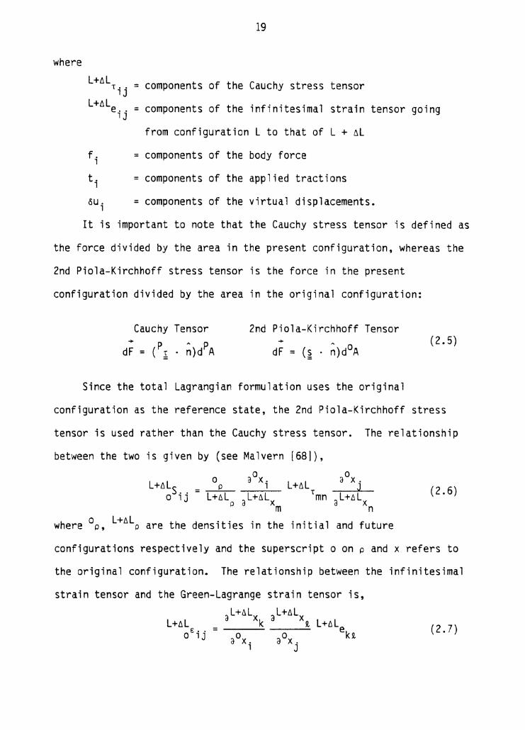
where L+til components of the Cauchy stress tensor T • • =

1 J L+til components of the infinitesimal strain tensor going e .. = lJ

from configuration L to that of L + til

f. = components of the body force 1

ti = components of the applied tractions

OU. 1 = components of the virtual displacements.

It is important to note that the Cauchy stress tensor is defined as

the force divided by the area in the present configuration, whereas the

2nd Piola-Kirchhoff stress tensor is the force in the present

configuration divided by the area in the original configuration:

Cauchy Tensor 2nd Piela-Kirchhoff Tensor -+- p A p

dF = { ~ · n)d A (2.5)

Since the total Lagrangian formulation uses the original

configuration as the reference state, the 2nd Piola-Kirchhoff stress

tensor is used rather than the Cauchy stress tensor. The relationship

between the two is given by (see Malvern [681),

a0 x. (2.6)

o L+6.L where p, o are the densities in the initial and future

configurations respectively and the superscript o on p and x refers to

the original configuration. The relationship between the infinitesimal

strain tensor and the Green-Lagrange strain tensor is, aL+tlLX al+6.Lx

L+til k ~ L+6.L o£ij = -ao_x_._ o ek~

1 a x j ( 2. 7)

20

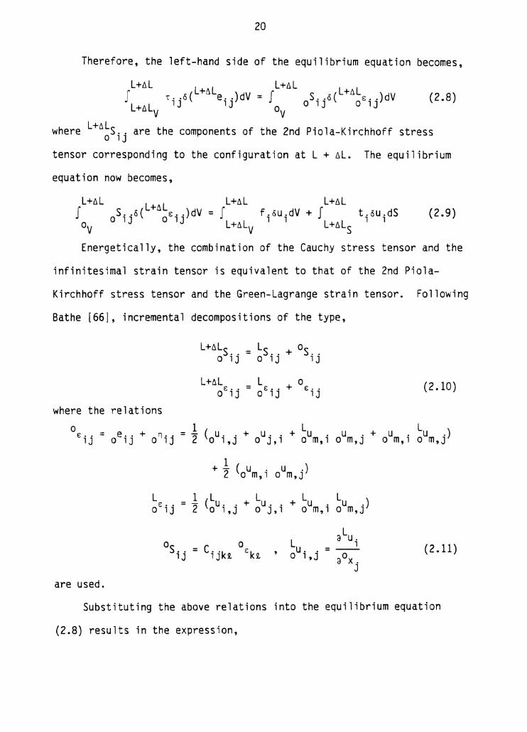
Therefore, the left-hand side of the equilibrium equation becomes,

L+ti.L L+ti.L J ' .. a ( e .. )dV L+ti.L lJ lJ v

L+ti.L L+ti.L = J s .. a( s .. )dV

0 0 lJ 0 lJ v

(2.8}

L+ti.L where S .. are the components of the 2nd Piola-Kirchhoff stress 0 1 J

tensor corresponding to the configuration at L + ti.L. The equilibrium

equation now becomes,

L+ti.L L+ti.L J s .. a( e .. )dV 0 0 lJ 0 lJ v

L+ti.L f .ou.dV + J 1 , L+ti.L s

t. OU .dS 1 1

(2.9)

Energetically, the combination of the Cauchy stress tensor and the

infinitesimal strain tensor is equivalent to that of the 2nd Piola-

Kirchhoff stress tensor and the Green-Lagrange strain tensor. Following

Bathe [66], incremental decompositions of the type,

L +ti.LS .. L 0 = s .. + s .. 0 lJ 0 1 J 1 J

L+tiL L 0 (2.10} E • • = E • • + E •• 0 1 J 0 1 J lJ

where the relations 0 = -21 ( u . . + u . . + Lu . u . + u . Lu ) sij = oeij + onij o l,J o J,1 o m,1 o m,J o m,1 o m,j

are used.

+ _21 ( u . u .) o m,1 o m,J

OL e ,. J. = _21 (Lu . . + Lu . . + Lu . Lu . ) o i,J o J,1 o m,1 o m,J

L u . . 0 l,J a0 x.

J

(2.11)

Substituting the above relations into the equilibrium equation

(2.8) results in the expression,

21

L+t.L L+6L J (L o o s .. + s .. )o{ E· .)dV 0 lJ lJ lJ av

= J f .ou.dV + J tiouidS L+t.Lv , 1 L+6Ls

or, upon rearrangement,

L+t.L = J

L+t.LV f .ou .dV , ,

L+t.L L + f t.ou.dS - J S .• o( e .. )dV L+6L , , o o lJ o lJ

s v At this point, linearization of the equilibrium equation is

desirable in order to get a form suitable for finite element

implementation. The assumptions made are, 0

E •• = e .. , J 0 , J

Substituting these relations into Eq. (2.13), we obtain

J C .. k ek o( e .. )dV + J Ls .. o( n •. )dV 0 lJ i 0 i 0 lJ 0 0 lJ 0 lJ v v

L+6L J L+6L f L f.ou.dV + t.ou.dS - S .. o{ e .. )dV 1 1 LHL 1 1 0 o lJ o lJ

s v

(2.13)

(2.14)

This is the form of the equilibrium equation which will be used to

construct the 3-0 degenerated shell element.

2.2 Finite Element Geometry and Formulation

The geometry of the element is presented here in detail following

Zienkiewicz [69J. The coordinates of a typical point in the shell

element (see Figure 2.1) are given by,

n (1 + ~ 3 ) (1 - ~ 3 ) xi= E ~J.(~ 1 ,~ 2 )[ 2 (x.). + 2 (x.). ]

j=l J 1 top J 1bottom (2.15)

22

.; 3

Node j

Global

Figure 2. l Local and global coordinate systems used in the 3-D degenerate shell finite element.

23

where

4>· =shape function associated with the element J

t; 1,t;2,t; 3 =normalized curvilinear coordinates

(x .). =global coordinate in the ;th direction at node j J 1

n = number of nodes in the element

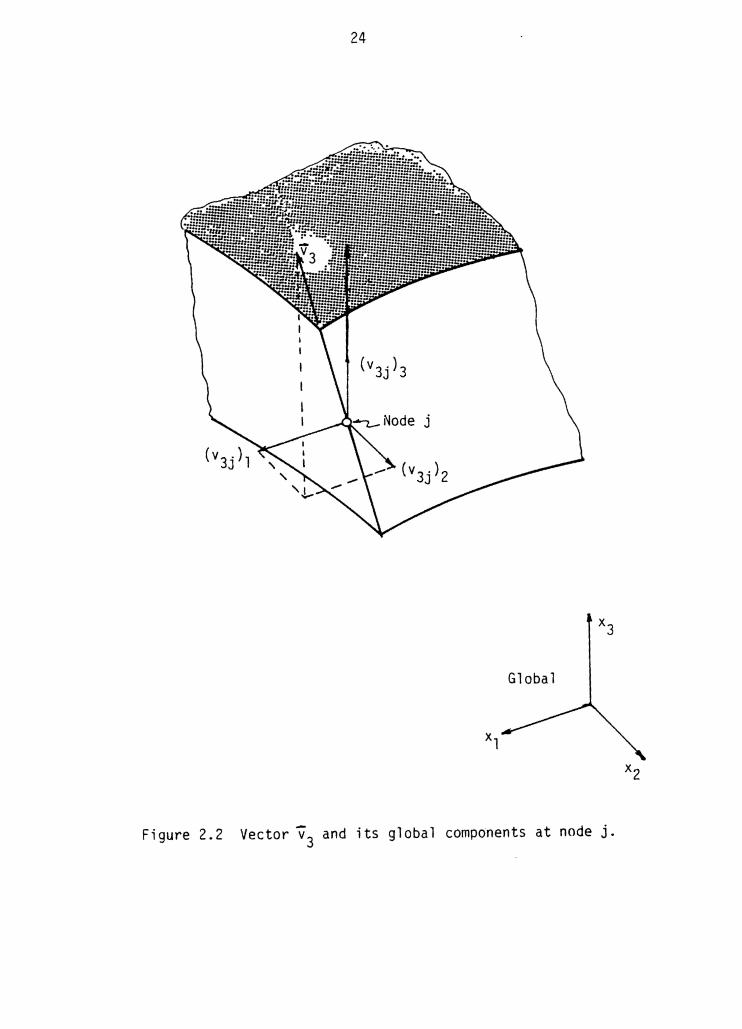
At node j, define a vector v3 such that,

e3j = v/lv31 (2.16)

The components of v3 at node j in the ;th global direction are then

(see Figure 2.2),

(v3 .). = (x.). - (x.). . J 1 J 1 top J 1bottom

(2.17)

Notice that the following relations also hold:

1 = -2 [(x.). - (x.). ] J 1 top J 1bottom

E:3 =-2 [(x.). - (x.). ]

J 1 top J 1bottom (2.18)

Hence, a typical point in the element can now be described by the

expression

x. = 1

(2.19)

A

Denote the components of vector e3 at node j along the global x;-axis as

A

(v3 .). = h./le3 .I. J 1 J J 1 (2.20)

where hj is the magnitude of v3, or the thickness of the element at node

j. The coordinates of a point in the element now became

n + t: 3h j I I x. = r <t>.(t;l,t;2)[(x.). 2 e3J" i]. 1 j=l J J 1 mid

(2.21}

24

Global

Figure 2.2 Vector V3 and its global compdnents at node j.

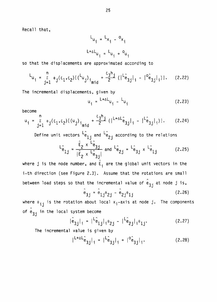
Recall that,

25

L+~Lu. =Lu. + ou. l l l

so that the displacements are approximated according to

L n L c;3h j LA oA u. = i: <t> • ( t; 1, c; 2)[ ( u . ) . + 2 ( I e3 . I . - I e3 . j • ) l . 1 j=l J J 1mid J 1 J 1

The incremental displacements, given by L+~L

U i = Ui

become n t;3hj L+~LA LA

u. = r qi.(c;l,c;2)[(u.). + 2 (j e3.j. - I e3.j.)]. 1 j=l J J 1mid J 1 J 1

(2.22)

(2.23)

(2.24)

Define unit vectors L~lj and L~2 j according to the relations A LA

LA E2 x e3j LA LA LA e1j = A LA and e2j = e3j x e1j (2.25)

IE2 x e3jl A

where j is the node number, and E. are the global unit vectors in the l

i-th direction (see Figure 2.3). Assume that the rotations are small A

between load steps so that the incremental value of e3j at node j is,

e3j = e1je2j - e2jelj (2.26)

where e .. is the rotation about local X·-axis at node j. The components 1 J 1

A

of e3j in the local system become A LA LA I e3 . j • = I e1 . j • s2 . - I e2 ·I . e 1 .• Jl Jl J Jl J

(2. 27)

The incremental value is given by L+~LA LA OA I e3jli = I e3jli + I e3jli. (2.28)

26

" Global E3

Figure 2.3 Element (local) and global unit vectors

27

Substituting Eq. (2.28) into Eq. (2.24), one obtains

n ; 3h. LA LA u . = l: <1> • ( E; 1, E; 2) [ ( u . ) . + -=..:u.2 ( I e 1 . J . e 2 . - I e2 . J . e 1 . ) l . ( 2. 29)

1 j=l J J 1mid J 1 J J 1 J

Therefore, the displacements, in going from the configuration at L

to that at L + ~L, are known when (uj)imid' e1j and e2j are known.

The development of the element equilibrium equations follows the

work of Chao and Reddy [2]. The vector {u} is defined as the column of

displacements at a node in the element and is related to the midplane

displacements and rotations, {~} according to

{u} = [T] (2.30)

(3 x 1) (3 x 5n) (5n x 1)

where, [T] is the transformation matrix defined by the incremental

displacement equation and n is the number of nodes in the element. The

strain-displacement equations for linear strain are

{oe} = L[A] {uo}

where

(2.31)

T {u } = { u u u u u U u u 0 u3, 3} 0 0 1,1 0 1,2 0 1,3 0 2,1 0 2,2 0 2,3 0 3,1 0 3,2 the derivatives are taken with respect to the original configuration,

and L[A] is the matrix relating eij to ui,j:

28

L 0 0 L l+ ul,l u2,l 0 0

0 L ul ,2 0 0 L 1+ u2,2 0

0 0 L 0 0 L

L[A] = ul, 3 u2,3

(6x9) L L 0 L L 0 ul,2 1+ ul,1 1+ u2,2 u2,1

L 0 L L 0 L ul,3 1+ ul,1 u2,3 u2,l

0 L L 0 L L ul ,3 ul ,2 u2,3 1+ u2,2

L u3,l 0 0

0 L u3,2 0

0 0 L 1+ u3,3 L u3,2

L u3,1 0

L 1+ u3,3 0 L

u3,l

0 L 1+ u3,3 L u3,2 (2.32)

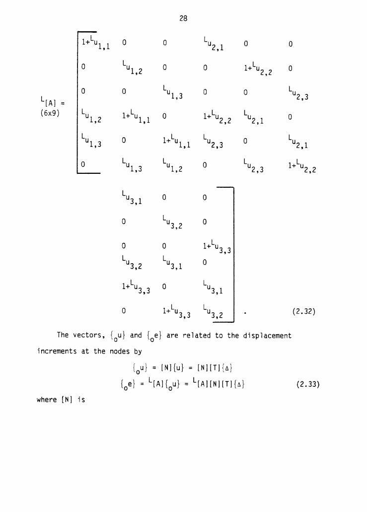
The vectors, {0 u} and {0 e} are related to the displacement

increments at the nodes by

{Ou} = [NJ{u} = [N][Tl{ll}

{0 e} = L[A]{0 u} = L[A][N][T]{~} (2.33)

where [N] is

29

a 0 0 ax 1 a 0 0 ax2 a 0 0 ax3

0 a ax 1

0

[NJ = 0 a 0 ax2

0 a 0 ax3

0 0 a ax1

0 0 a ax2

0 0 a ax3

{2.34)

Then the [B] matrix can now be formed as,

[BJ= L[A][NJ[TJ (2.35}

so that,

{0 e} = [BJ{ti}. (2.36)

Using the definition of the [BJ matrix and substituting it into Eq.

(2.13), one obtains

(2.37)

where L[KLJ, l[KNLJ' L+til{R}, L+til{F} are the linear and non-linear

stiffness matrices, the external force vector, and the unbalanced force

vector, respectively. Explicitly,

~

30

L[KL] =I ov

L[KNL] =I ov

L+6L{F} = [ ov

(2.38)

where [S] and {S} are the matrix and vector forms of the 2nd Piola-

Kirchhoff stress tensor.

2.3 Material Nonlinearity

The inclusion of material nonlinearity into the analysis becomes

essential to accurately predict stress states well above yield stress

levels. In this study, the material nonlinearity will be modelled by

using the associated flow rule with isotropic work hardening. The

associated flow rule states that the plastic strain is related to the

stress in the following manner:

(2.39)

where \ is a constant, and

{de}pl = incremental plastic strain components

F = yield function (modified Von Mises)

{o} = vector of the components of stress.

Recalling that elastic strains can be found from the derivative of

the elastic strain energy density function with respect to the

appropriate stress components, it is seen that the associated flow rule

will yield plastic strain increments in a similar manner where the yield

function serves as a plastic potential.

31

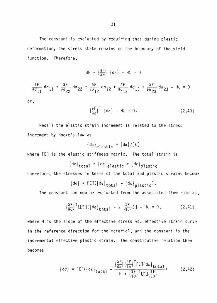
The constant is evaluated by requiring that during plastic

deformation, the stress state remains on the boundary of the yield

function. Therefore,

or,

(2.40)

Recall the elastic strain increment is related to the stress

increment by Hooke's law as

{dE}elastic = {dcr}/[E]

where [E] is the elastic stiffness matrix. The total strain is

{ddtotal = {dE}elastic + {dE}plastic

therefore, the stresses in terms of the total and plastic strains become

{dcr} = [EJ({dE}total - {dE}plastic).

The constant can now be evaluated from the associated flow rule as,

(2.41)

where H is the slope of the effective stress vs. effective strain curve

in the reference direction for the material, and the constant is the

incremental effective plastic strain. The constitutive relation then

becomes

{dcr} = [E]({dE}total -aF aF T

{ctcrHaa} [EJ{ dE}total) H + {~}T[EJ{~} ocr - oa

(2.42)

32

or,

where

(2.43}

Hence, for plastically behaving Gauss points, the second term on

the right hand side is evaluated, and for elastically behaving Gauss

points, this term is set to zero.

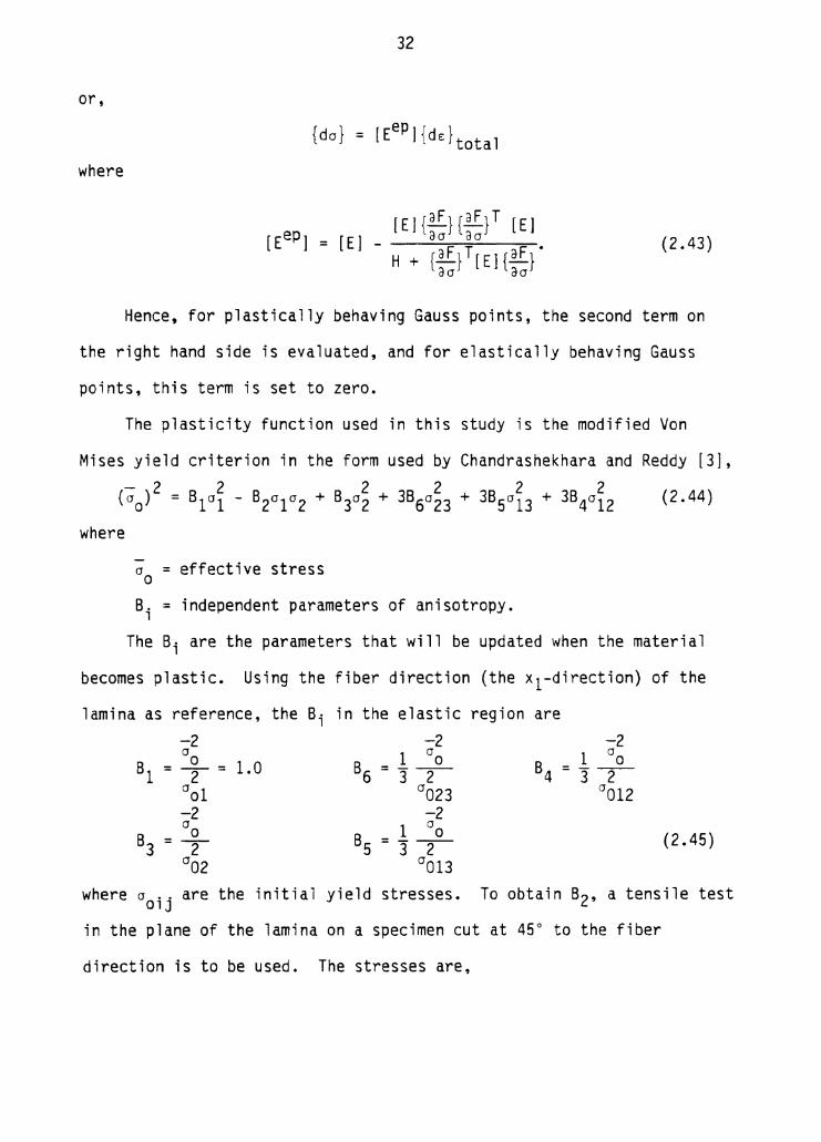
The plasticity function used in this study is the modified Von

Mises yield criterion in the form used by Chandrashekhara and Reddy [3],

(-cr0 ) 2 B 2 B B 2 38 2 38 2 38 2 (2 44) = 1°1 - 2°1°2 + 3°2 + 6°23 + 5°13 + 4°12 • where

a0 = effective stress

B. = independent parameters of anisotropy. l

The Bi are the parameters that will be updated when the material

becomes plastic. Using the fiber direction (the x1-direction) of the

lamina as reference, the Bi in the elastic region are -2 a

s1 = + = 1.0 0 ol -2 oo

83 = 2 0 02

-2 1 °o 86 = 3 -2-

0023 -2

1 °o 85 = 3 -2-0013

-2 1 °o

84 = 3-2-0012

(2.45)

where croij are the initial yield stresses. To obtain s2, a tensile test

in the plane of the lamina on a specimen cut at 45° to the fiber

direction is to be used. The stresses are,

33

1 al = a2 = al2 = 2 a045

a23 = a13 = 0 (2.46)

where cr045 is the initial yield strength of the lamina in the 45°

direction. Therefore,

or, -2 -2 cro cro

+-2-+-2--002 °012

-2 a

4 _0_ 2

0045 The plastic anisotropic parameters are found using the work

(2.47)

hardening rule which states that the plastic work done by each stress

component will be the same. Let, H a 1 = uniaxial yield stress in the x1 direction including

hardening effects

cr = corresponding effective stress p El = plastic strain in the x1 direction

EPl = slope of the stress vs. plastic-strain curve in the x1 direction

For cr~ and cr~ to correspond to the same effective stress, a, the

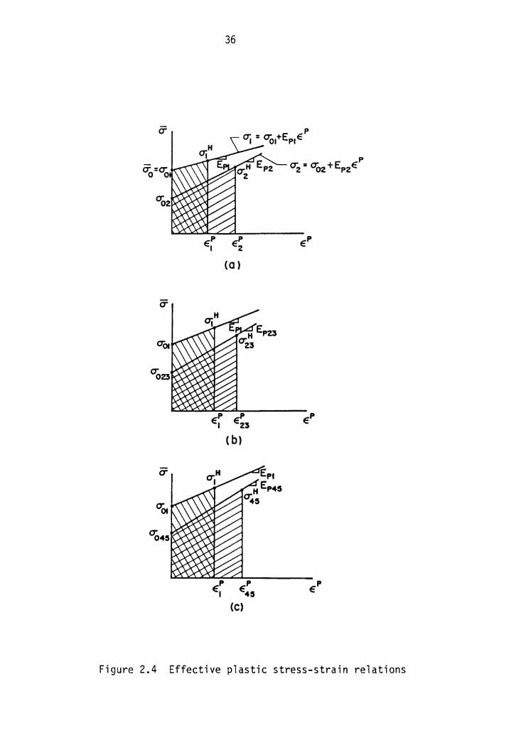
work done should be the same. Therefore, from Figure 2.4a, one obtains,

(2.48)

Note that,

34

Therefore,

or

=

so,

E ( H)2 _ __fg_ [( H)2 a2 - E al

Pl (2.49)

Since the reference direction is the x1-direction, s1 = 1.0, and - H therefore a= a 1. Hence,

so the plastic s3 is

-2 -2 8 = a = -=------a _____ _

3 (aH2)2 EP2 - 2 2 2 -E- [(a) - (aol) l + (a02)

Pl Similarly, using Figure 2.4b,

-2 -2 8 = a o = G 6 3(0~3)2 2 2 3 [ P23 (;-2 001) + (0023) l EPl

-2 -2 8 = o o = G 5 3(0~3)2 2 2 3 [ Pl3 (-;-2 - 001) + (0013) l EPl

-2 -2 8 = a a =

GP12 -2 2 4 3(a~2)2 2 3[-E- (a - aOl) + (0012) l Pl

(2.50)

(2.51)

(2.52)

(2.53)

35

For B2, use Figure 2.4c and recall that elastically -2

H where 0 045 becomes

Therefore, we have

00 B2 = 1 + B3 + B4 - 4 H 2

<0 045)

-2 4o

(2.54)

(2.55)

The independent anisotropic parameters vary as a function of

plastic strain (they do not change if no plastic strain occurs). In

general, the stresses will be calculated in the material principal axes

system, so that the stresses must be transformed from the global axes as

fol lows:

cos2e . 2 2a sine case al = a + a sin e + x y xy

a2 = a x sin2e + a y cos2e - 2a sine xy case

0 23 = -a xz sine + a yz COSS

cr13 = 0 xz case + a yz sine

0 12 = -o x sine case + oy sine case + crxy(cos2e sin2e). (2.56)

As mentioned earlier, the stress state must remain on the boundary

of the plasticity function in order to evaluate the plastic strains.

36

(a)

Figure 2.4 Effective plastic stress-strain relations

37

The scheme to reduce the stresses to the boundary at each load step in

the program will be the one used by Chandrashekhara and Reddy [3].

2.4 Computational Procedure

The total load is divided into a number of load steps. At each

load step, the global stiffness matrices and force vectors are

assembled, boundary conditions are applied, and the solution vector is

calculated (see [70]). If the displacement solution is not within a

specified amount of error, an iteration process at this load step begins

using the full Newton-Raphson technique. Once the displacement solution

is obtained at this load level, the stresses and strains are calculated

at the top and bottom of each lamina at the Gauss points of the

element. Then the material nonlinearity is checked in each element at

each Gauss point. If no Gauss points of an element pass the criterion,

the element stiffnesses are reduced. After all elements are checked,

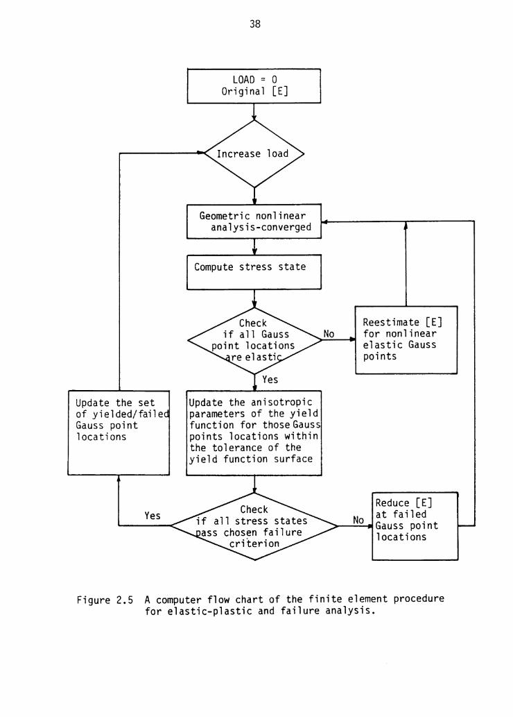
the load step is increased, and the process is repeated. A flow chart

of the general procedure is shown in Figure 2.5.

If, after the geometric nonlinearity has converged, it is found

that a Gauss point is not elastic, a re-estimation of the stiffnesses

get this Gauss point 1 s stress state on the yield function surface is

done. The same load step is rerun until all of the Gauss point stress

state are at least on the surface of their respective yield functions.

The failure criterion is then checked.

When the failure criterion is violated, the failed constitutive

matrix at that Gauss point, of that lamina, in that element is set

nearly to zero. This is to reflect the fact that for at least some

to

Update the set of yielded/faile Gauss point locations

Yes

38

LOAD = 0 Original [E]

Geometric nonlinear analysis-converged

Compute stress state

Update the anisotropic parameters of the yield function for those Gauss points locations within the tolerance of the yield function surface

Reestimate [E] No for nonlinear

elastic Gauss points

Reduce [E] No at failed

~-.;.;.;;..-111Gauss point locations

Figure 2.5 A computer flow chart of the finite element procedure for elastic-plastic and failure analysis.

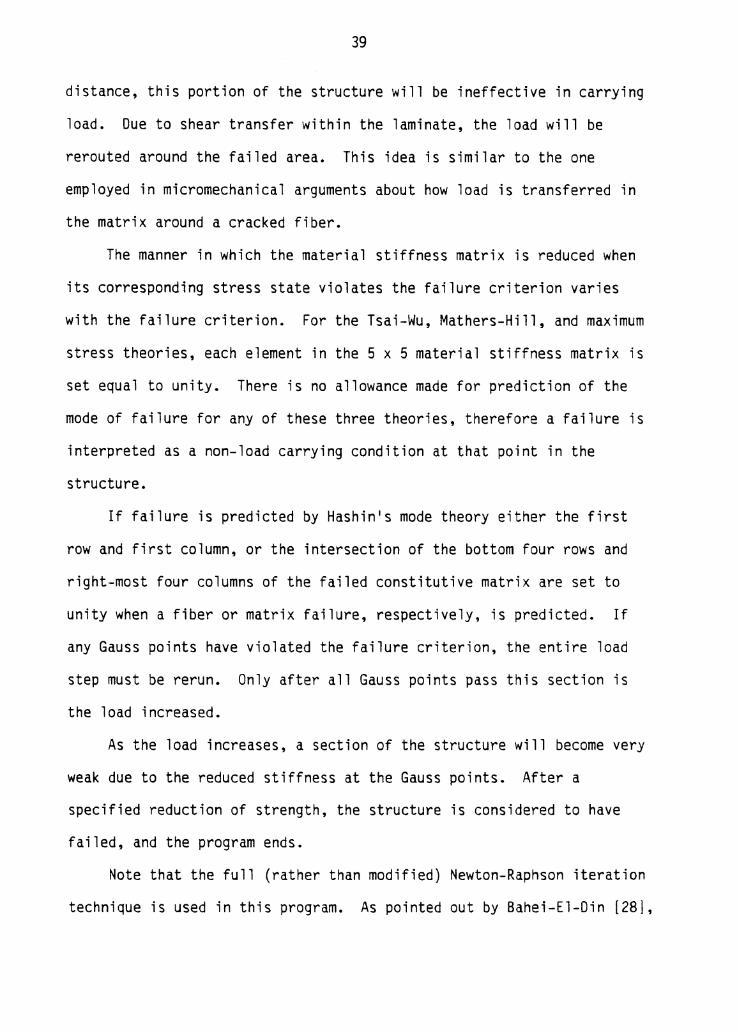
39

distance, this portion of the structure will be ineffective in carrying

load. Due to shear transfer within the laminate, the load will be

rerouted around the failed area. This idea is similar to the one

employed in micromechanical arguments about how load is transferred in

the matrix around a cracked fiber.

The manner in which the material stiffness matrix is reduced when

its corresponding stress state violates the failure criterion varies

with the failure criterion. For the Tsai-Wu, Mathers-Hill, and maximum

stress theories, each element in the 5 x 5 material stiffness matrix is

set equal to unity. There is no allowance made for prediction of the

mode of failure for any of these three theories, therefore a failure is

interpreted as a non-load carrying condition at that point in the

structure.

If failure is predicted by Hashin 1 s mode theory either the first

row and first column, or the intersection of the bottom four rows and

right-most four columns of the failed constitutive matrix are set to

unity when a fiber or matrix failure, respectively, is predicted. If

any Gauss points have violated the failure criterion, the entire load

step must be rerun. Only after all Gauss points pass this section is

the load increased.

As the load increases, a section of the structure will become very

weak due to the reduced stiffness at the Gauss points. After a

specified reduction of strength, the structure is considered to have

failed, and the program ends.

Note that the full (rather than modified) Newton-Raphson iteration

technique is used in this program. As pointed out by Bahei-El-Din [28],

Attention Patron:

Page _____ omitted from

numbering

40

41

Third, the stress states are computed on the 2x2 Gauss point grid

within each element since full, 3x3 Gauss quadrature is used to compute

the displacement solution.

Fourth, there are two material stiffness matrices at each Gauss

point location in each lamina in each element. Therefore, there are a

total of [(NOE - l)*NOL*l3 +(NOL - 1)*13 + 13] constitutive matrices

per model.+ These matrices are the ones being manipulated by the

plasticity and failure theory subroutines.

Fifth, since there is, in general, a variation of material

properties through the thickness of each lamina in an element, the

integration in this direction must be modified. The integration through

the thickness is now carried out over half of each lamina using the

appropriate material stiffness matrix. For example, to integrate

through the thickness of a laminate composed of N layers, the integral

ff f [B]T[Q][B]d~d~dn n ~ ~

where [BJ is in general a function of ~ becomes

2N ~k+l f f E f

k=l ~ k (2.57)

where N is the total number of layers and n = 0,1,2 in this study. Note

that there are two layers within each lamina, each having its own

material stiffness matrix. This allows the upper portion of a lamina to

act independently of the lower portion in the sense that the upper

portion may go plastic, while the lower one remains elastic. This

+where NOE = number of elements in the model NOL = number of layers in the model

42

approach is adopted because, in general, the stress states are most

severe at the top and bottom of each lamina.

2.6 Reducing Stress States to the Plasticity Function Surface

From the material nonlinear description one can define

so that the incremental effective plastic strain is

d°1 = [W]de:

and Hookes law generalized to the plastic region becomes

{da} = ([E] - [EJ{if}[w]){de:} aa or,

The technique to satisfy plasticity is to:

1) choose an [EeP]

2) compute displacements

3) compute the total and plastic strains

4) compute stresses

(2.58}

(2.59)

5) check to see that stress states satisfy the plasticity function

If not: a) reestimate [E] of the Gauss points that failed

b) repeat 2) through 5) until stresses are converged.

Now the [EeP] at hand satisfies the plasticity surface requirement and

stress-strain relations in elastic and plastic regions. When using

linear strains, one can get the stress states back down to the

plasticity function surface by setting up a scalar factor

43

xm = 1 0 computed

For the incremental effective plastic strain,

d;P = [W]{dE}(xm)

(2.60)

where {ds}(xm) is the elastic portion of the total strain and the

modified Hooke 1 s law is

{de} = ([E] - (xm)[E]{2l-}[W]){dE} aa (2.61)

where

[Eep] = ([E] - (xm)[E]{lt.}[W]). ac (2.62)

Notice the role of xm; it tells one how much of the strain is

elastic and how much is plastic. This is necessary to know when

computing the effective plastic strain increment, and eventually, the

individual plastic strain increments. It is not necessary to know how

much of the total strain is elastic or plastic when computing the

incremental stresses. However, when linear strains are used, it is

convenient to use xm as shown above.

When nonlinear strains are used, there is no guarantee that the use

of xm will lead to convergence. The displacements, computed using the

reduced stiffnesses, may cause strains that are high enough to produce

an increased stress state. One expects greater displacements and

strains due to the decreased stiffnesses, but one also expects decreased

stress states for the same reason. The use of xm with linear strains

gives the expected results; with nonlinear strains, in general, it

fails, or requires smaller load steps, for the continuum based element.

Attention Patron:

Page _____ omitted from

numbering

44

Attention Patron:

Page _____ omitted from

numbering

45

CHAPTER 3

NUMERICAL RESULTS

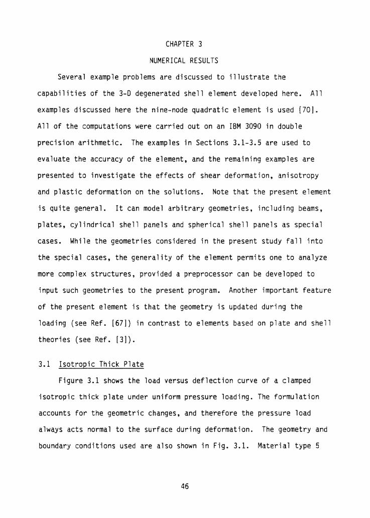
Several example problems are discussed to illustrate the

capabilities of the 3-D degenerated shell element developed here. All

examples discussed here the nine-node quadratic element is used [70).

All of the computations were carried out on an IBM 3090 in double

precision arithmetic. The examples in Sections 3.1-3.5 are used to

evaluate the accuracy of the element, and the remaining examples are

presented to investigate the effects of shear deformation, anisotropy

and plastic deformation on the solutions. Note that the present element

is quite general. It can model arbitrary geometries, including beams,

plates, cylindrical shell panels and spherical shell panels as special

cases. While the geometries considered in the present study fall into

the special cases, the generality of the element permits one to analyze

more complex structures, provided a preprocessor can be developed to

input such geometries to the present program. Another important feature

of the present element is that the geometry is updated during the

loading (see Ref. [67]) in contrast to elements based on plate and shell

theories (see Ref. [3]).

3.1 Isotropic Thick Plate

Figure 3.1 shows the load versus deflection curve of a clamped

isotropic thick plate under uniform pressure loading. The formulation

accounts for the geometric changes, and therefore the pressure load

always acts normal to the surface during deformation. The geometry and

boundary conditions used are also shown in Fig. 3.1. Material type 5

46

Load p

47

100

80. 0 Present study

() Reference [3] 60.

qo a4 y p =

Eh4 40. 4 u=O

E = 2xl0 MPa el=O v = 0.3

20. x a = lm v=e =O a , .. 2a~ h= 10

0.0 0.0 0. 19 0.38 0.56 0.75 0.94 1. 13 1. 31 1. 50

Nondimensionalized center deflection, (-w/h)

Figure 3o 1 Bending of a clamped square plate {isotropic) under uniform transverse load of intensity q0 {a/h=lO).

48

(see Appendix) is used. The side length to thickness ratio is ten.

Good correlation with the results of reference [3] is observed.

3.2 Orthotropic and Cross-Ply Thin Plates

Clamped orthotropic and cross-ply square plates under uniform

pressure load are analyzed, and the load versus deflection curves are

compared in Figure 3.2 with the results from reference [3], which is

based on a shell theory. The plate has a side length to thickness ratio

of 500, and made of material type 4. Notice that both plates have large

geometric nonlinear effects even when centerline deflections are only

one and a half times the plate thickness. The difference between the

present solution and that of Ref. [31 is possibly due to the fact that

the present formulation accounts for geometric changes during

deformation.

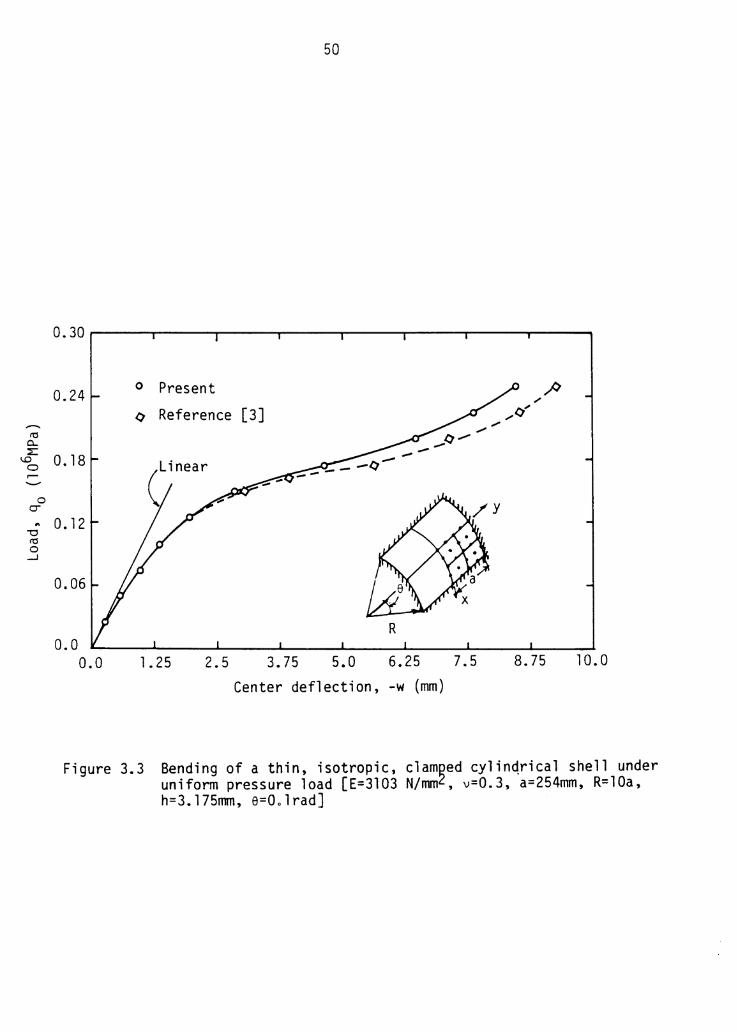
3.3 Isotropic Cylindrical Shell Panel

Figure 3.3 shows the load versus centerline deflection of a

clamped, thin cylindrical shell panel of material type 6 under a uniform

pressure load. The present results show a greater 11 softening 11 than that

in Ref. [3]. Again, this is due to the fact that the present element

accounts for geometric changes during loading. Good agreement is

observed, as both show an eventual stiffening of the panel.

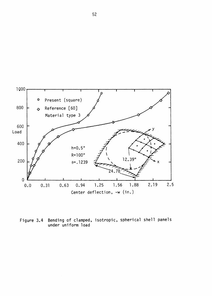
3.4 Isotropic Spherical Shell Panel

A square edged isotropic spherical shell panel, or an end cap, is

analyzed and the results are compared to the results of a circular-edged

shell (see (60]) of material type 3 with clamped boundary conditions in

'° a.. :E:

<::!'" 0

.08

.::. . 06 0

CT

~

~ .04 0

_J

.02

49

0 Present ! Orthotropic <> Reference [3]

• Present l (oo;goo)

+ Reference [3] f

Dimensionalized center deflection (mm)

4.38 5.0

Figure 3.2 Bending of orthotropic and cross-ply (0°/90°), clamped square laminates under uniform distributed transverse load (q ) 4 2 [a=l,000 mm, h=2 mm, E 1 ~12.sE2 , E2=2xl04 N/mm2, G12=G 23Q 10 N/mm

4 2 G23=0"4xl0 N/mm ,v 12= 0.275]

l'C c... :::c

"° 0 r-

0 0-.. -0 l'C 0 _J

0.24

0. 18

0. 12

0.06

0.0 0.0

0 Present () Reference

1.25 2.5

50

ft /

[3] ¢' "' .... ,.

R

3.75 5.0 6.25 7.5 8.75 10.0 Center deflection, -w (mm)

Figure 3.3 Bending of a thin, isotropic, clam~ed :ylinqr~cal shel~ under uniform pressure load [E=3103 N/mm , v-0.3, a-254mm, R-lOa, h=3. 175mm, e=O.lrad]

51

Figure 3.4. The circular shell cap fits inside the square shell panel,

and thus one expects a stiffer response from the square shell panel.

Both spherical shells undergo twelve load steps of 80 psi. The response

of each shell is similar, with the circular shell of Ref. [601 being

"softer~ as expected. Both shells show the hardening effect after an

initial softening effect.

3.5 Combined Nonlinear Effects on thin Cylindrical Shells

An isotropic, clamped, thin (a/h = 160) cylindrical shell panel

under uniform pressure loading is analyzed to determine the effect of

the material nonlinearity on the deflection. Material type 7 is used

(low yield stress, perfectly plastic behavior).

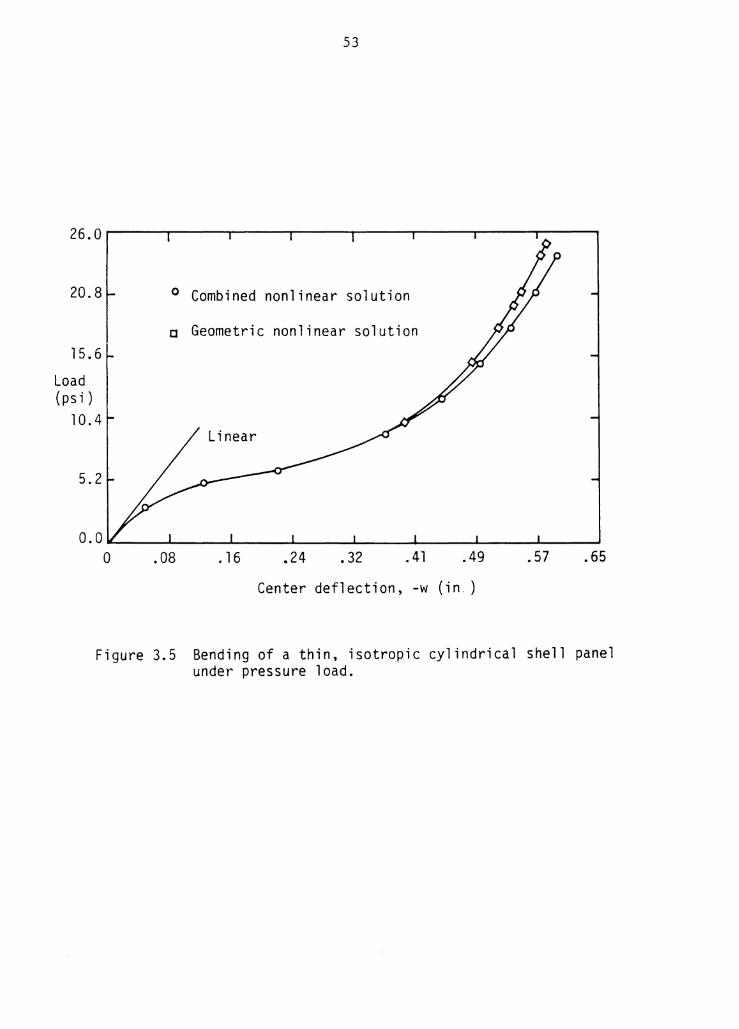
Figure 3.5 contains the plots of the load versus centerline

deflection for linear, geometric nonlinear, and combined geometric and

material nonlinear cases. Note that the shell panel exhibits the same

general behavior as was previously shown in Figure 3.3; an initial

softening followed by stiffening of the structure. The material

nonlinearity does not affect the solution appreciably until the

stiffening action occurs. When stiffening does occur, the cylindrical

shell behaves in a similar fashion to a flat plate; the material

nonlinearity softens the shell panel while the geometric nonlinearity

stiffens the shell.

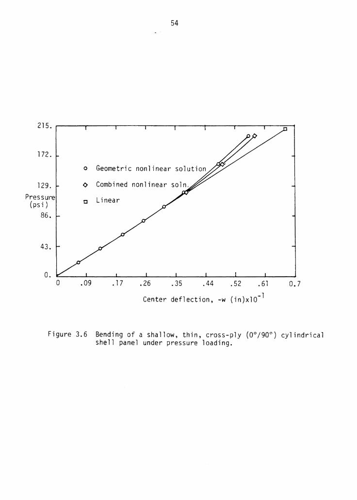
Results of the combined nonlinearity on a cross-ply, thin, shallow

shell panel are presented in Figure 3.6. The shell panel is made of

material type 2. The edges are clamped and a uniform pressure load is

applied. The side length-to-thickness ratio is 32. Note that the

1000

800

600 Load

40a

200

0 a.a

0

¢

52

Present (square) Reference [60] Material type 3

h=a.5" R=l00 11

8=01239

0. 31 0.63 a.94 1.25 1. 56 1. 88 2. 19 2.5 Center deflection, -w (in.)

Figure 3.4 Bending of clamped, isotropic, spherical shell panels under uniform load

53

20.8 ° Combined nonlinear solution

15.6

Load (psi )

10.4

5.2

0

a Geometric nonlinear solution

.08 . 16 .24 • 32 . 41 .49

Center deflection, -w (in,)

.57 .65

Figure 3.5 Bending of a thin, isotropic cylindrical shell panel under pressure load.

54

172.

o Geometric nonlinear solution

129. ¢ Combined Pressure

(psi ) 86.

43.

0.

c Linear

a .09 . l 7 .26 .35 .44 .52 • 61

( . ) - l Center deflection, -w in xlO

0.7

Figure 3.6 Bending of a shallow, thin, cross-ply (0°/90°) cylindrical shell panel under pressure loading.

55

shallow shell panel exhibits entirely different behavior than the

isotropic shell panel discussed in the preceeding paragraphs. The

behavior is very much like that of a flat plate, with the geometric

nonlinear effect dominating the material nonlinear effect through the

entire load range considered here. From the results, it is noted that

the matrix in both lamina went plastic first at the top and bottom of

the panel near the center.

3.6 Plate Strip

A cantilever plate strip is used to investigate the full geometric

and material nonlinear effects on failure analysis. Isotropic,

orthotropic, and cross-ply plate strips are examined, with the failure

theories being applied to the latter two cases. Also, a two-layer

angle-ply (45°/-45°) plate strip was analyzed to evaluate the failure

criteria. Two layers are used in the analysis, therefore four through-

the-thickness constitutive matrices are employed at each Gauss point

(see Fig. 3.7).

3.6.l Isotropic Plate Strip

First, the isotropic plate strip results are discussed. As the

load was applied, the Gauss points nearest the wall of the seven element

plate strip (see Fig. 3.7), on top and bottom of the structure, exhibit

plastic deformation between load values 400 and 600 psi. Based on the

magnitude of the scale factor xm, the Gauss points at the top of the

plate went plastic first. As the load was further applied, the material

nonlinear effect began to dominate the geometrically nonlinear effect.

56

Nodes

-----5"-----------Through-th-thickness material stiffness locations

(a) Seven element discretization

Stresses are computed at the top and bottom of the layer at the Gauss points

~-+-~--'r--+----'li-----+-----:-~

.__.__. _ _.__.___._ _________ ....._ _____ x

Node

(b) Eight element discretization

Figure 3.7 Geometry and finite element meshes used in the plate strip problems

57

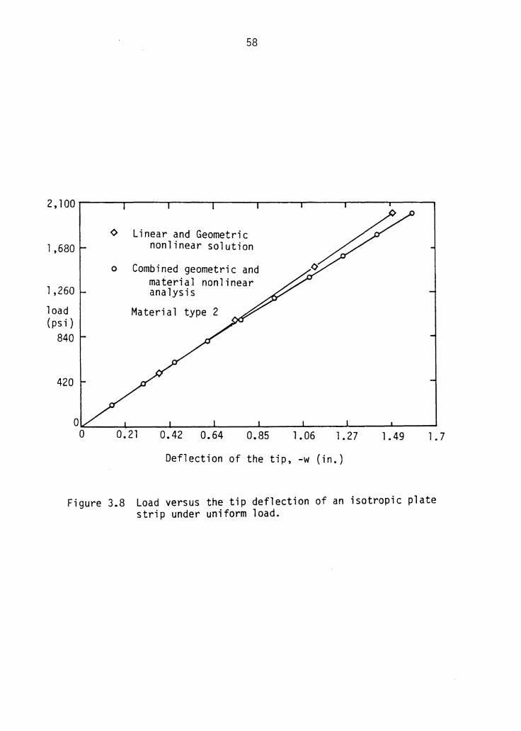
Figure 3.8 shows the deflection of the tip of the plate strip as a

function of the applied load. When only geometric nonlinearity is

included, the plate strip stiffened slightly, and when both

nonlinearities are included, a softening is seen to take place. The

deformed positions at the maximum load (2,000 psi) are shown in Figure

3.9 for the cases of geometric and geometric/material nonlinear

effects. Again, the material effect is clearly present.

Figure 3.10 contains a plot of stress versus load for the same

problem. The plot shows the stress predictions at the Gauss points

nearest the wall on the bottom of the plate with and without the

material nonlinearity. First, notice that the effective stress,~' is

very close to the yield stress at all load levels (5% tolerance was

used). Second, the curves show the predicted bending stresses with and

without material nonlinear effect. Clearly, for this thick isotropic

plate strip, neglecting the material nonlinear effect would be

unadvisable as failure would be predicted far too soon based on the

geometrically nonlinear description alone. If a thin plate were used,

one can argue that the geometric effect will overwhelm the material

effect in most cases. This is true, but near failure, the material

effect will again emerge.

3.6.2 Orthotropic Plate Strip

The same physical dimensions as those used for the isotropic plate

strip are used here, but the mesh now contains eight elements to better

define the behavior near the wall. Material type 2 was used.

1 ,680

1 ,260 load (psi)

840

420

¢

0

58

Linear and Geometric nonlinear solution

Combined geometric and material nonlinear analysis

Material type 2

0.21 0.42 0.64 0.85 1.06 1.27

Deflection of the tip, -w (in.)

1.49 l. 7

Figure 3.8 Load versus the tip deflection of an isotropic plate strip under uniform load.

• c ...... ........ 3

ft

c 0 ...... .µ u ~

....-4-~ Cl

59

o.o

-0.33

-0.67

-1.00 0 Geometric nonlinear solno

¢ Combined nonlinear solno

-1.33

-l.66 ....... ~~ .......... ~~~~~-'-~~-'-~~--'~~~.__~~...._~---o 0.63 1.25 1.88 2.5. 3.13 3.75 4.38 5.0

Figure 3.9

Distance along the length of the plate (in)

Deformed configuration of the isotropic plate strip under uniform pressure (at 2000 psi).

CV') 0 .-x -V1 a.

x 0 I

450

360

270

60

o Combined nonlinear soln.

a Geometric nonlinear soln.

Effective stre~s at G~uss point 10 tbottom)

Yield stress

~ 180 V1 V1 QJ ~ +-' V1

.-tO

x <(

90

0 0 100 200 300 400 500 600 700 800

Intensity of the pressure (psi)

Figure 3. 10 Nonlinear effects on the axial stress near the wall of the cantilevered plate strip (isotropic).

61

The same locations as in the isotropic case go plastic, but they do

so at a lower load level. This is due to the weak matrix tensile

strength relative to the shear strength of the isotropic materials.

Figure 3.11 shows that the overall behavior of the plate strip is

linear, even though plasticity occurred early in the load cycle. The

bending stresses are much higher in the orthotropic case, and indeed are

nearly equal to the fiber tensile strength (200,000 psi) at the 700 psi

load level as is seen in Figure 3.12. Therefore, one would expect a

nearly linear behavior until a fiber failure occurs. Indeed, this is

what is predicted by Hashin's mode criterion when the same loads are

used. The plasticity spread to a distance of nearly one inch in the

matrix in the x direction before a tensile fiber failure on top and a

compressive fiber failure on bottom (near the wall) were predicted at

the 700 psi load. After the failure and reduction of these constitutive

matrices, the tip deflection was found to be 1.5% greater than the value

when no failure was considered. No further load steps were run.

This example was again run using the Tsai-Wu failure criterion.

Again, failure was predicted in the same locations, top and bottom of

the strip at the wall, but here, the entire constitutive matrix was

reduced (as no mode prediction is possible). The solution would not

converge after failure with Tsai-Wu because no stiffness at all was left

on the top or bottom of the beam, even though fibers were still active

in the center. This says that the shear transfer was not sufficient to

reroute the loading path through the matrix to the fibers deeper inside

the strip. This observation of the distinction between the Hashin and

the Tsai-Wu criteria is relative to the model, load steps, and mesh

62

600 o Linear and nonlinear

450

-Ill c..

300 QJ 5-::::i Ill Ill QJ 150 5-

a..

0 0 .03 • 06 .09 . 13 • 16 • 19 .22 .25

Tip deflection, -w (in.)

Figure 3. 11 Load versus tip deflection of orthotropic plate strip under pressure loading. ·

63

640 o Linear and nonlinear solnsc

480

.,.... :g_ 320

0 26.25 52.5 78.75 105

Axial stress, -a x

131.25 157.5 183.75 210

(psi)x103

Figure 3. 12 Nonlinear effects on the axial (bending) stress near the wall of an orthotropic plate strip.

64

employed, so that the effect of trying to predict a mode of failure

rather than just occurrence of failure can be shown. This only means

that using Tsai-Wu a deflection of greater than 1.5% (over the no-

fai lure analysis) at the tip will be experienced and hence greater

strains. Leaving the matrix stiffnesses in (i.e. the Hashin criterion)

therefore, will start to show different numerical results than when the

matrix stiffness must be reduced (i.e. the Tsai-Wu criterion). This

results in the possibility of different load paths, and different gross

failure modes in examples where the structure geometry is more complex.

3.6.3 Cross-Ply Plate Strip

The same geometry and mesh as in the orthotropic plate strip was

used here except that the bottom quarter inch of the strip is made up of

a layer of 90° plies. One wouldn 1 t necessarily build this structure in

this manner, but it is instructive to look at how failure occurs and

what effect plasticity (material nonlinearity) has on it.

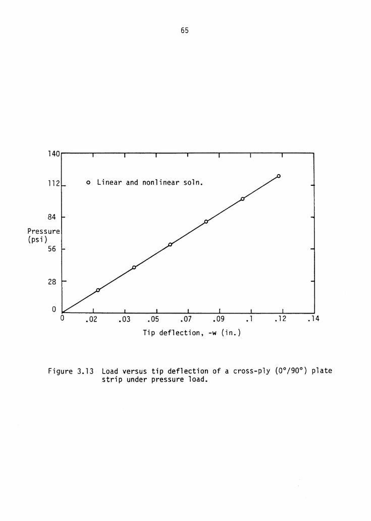
Figure 3.13 shows the plot of load versus deflection, which is

essentially linear. The loads are much smaller than the orthotropic

case as would be expected. The material effect is shown to have a

little more influence on the bending stress in the bottom (90°) ply.

The bending stress in the upper ply showed no appreciable material

effect as in the orthotropic case. Here, plasticity did not occur in

the (0°) ply. Plasticity started at the wall at a load of 40 psi and

grew to a distance of one and a half inches at the last converged

load. Another difference between the cross-ply case and the orthotropic

case is that the entire thickness of the (90°) ply went plastic. That

65

112 o Linear and nonlinear soln.

84

Pressure (psi)

56

28

0 0 .02 .03 .05 .07 .09

Tip deflection, -w (in.) • 1 • 12 • 14

Figure 3. 13 Load versus tip deflection of a cross-ply (0°/90°) plate strip under pressure load.

66

is, the bottom quarter inch of the structure for approximately 30% of

the strips length was plastic at the last load step. The stresses in

the matrix direction in the go 0 ply were also over their failure

strength, so that one could expect failure before this load level was

reached.

Both the Mathers-Hill and the maximum stress criteria predicted

failure near the wall in the go 0 ply at the 100 psi load level, then

farther from the wall at the 120 psi level. The deflections at the tip

however, were less than 6% over the case where no failure criterion was

employed. Therefore, even though failure was predicted (and the

constitutive matrices reduced) for the lower l/8 11 of the thickness of

the strip, the structure does not exhibit noticeable changes in stresses

and deflections. Therefore, the load path was not affected very much at

all, which is no surprise since the (0°) lamina is on top. The bending

stresses on the top do increase, but not dramatically, in taking up the

extra load.

3.6.4 Angle Ply (45°/-45°) Plate Strip

The thick plate strip used previously to show the effects of the

material nonlinearity is used again to evaluate the maximum stress,

Tsai-Wu, and Hashin 1 s failure criteria. All stress states are computed

using the geometric nonlinearity only. The loading used is the same as

before, namely, uniform pressure on the surface at all times. The load

step used was 10 psi until first failure occurred, then the computation

was terminated.

67

Both the maximum stress and the Tsai-Wu criteria predicted first

failure between 70 and 80 psi of load value at the same locations, at

the two Gauss points nearest the wall, top and bottom, and on opposite

sides (see Figure 3.14). Hashin 1 s criterion predicted failure at the

same load level, but only at the upper Gauss point. The mode of failure

is tensile matrix failure in the top lamina. At this same location the

maximum stress criterion was violated by a tensile normal stress in the

matrix direction (i.e. material x2-direction), and cr 2 stress was the

largest, as a percentage of its strength, in the Tsai-Wu criterion. At

the lower Gauss point, the same phenomenon occurred for the maximum

stress and Tsai-Wu criteria, except that the cr 2 stress was now in

compression.

The predicted failure locations are consistent with the mechanics

of composite material; the corners of the structure where the fibers of

each layer are short do not carry much of the load. It is reasonable to

expect a matrix failure in these regions. The results indicate this in

the corners opposite to where the failure occurred. The fiber is the

dominant load carrying member and the normal component of stress in the

matrix direction was about half of the value predicted at the failed

locations.

It is interesting to note that a noninteracting (no products of

different stress components) stress criterion (maximum stress) and an

interacting stress criterion (Tsai-Wu) predict failure at the same load

levels, both in compression and tension, at the same locations in the

structure. Recall that the interaction term, F12 , was set to zero in

the Tsai-Wu criterion, effectively taking away the stress interaction in

68

---- 45° - • ---- • -45° ---- . - (Front view) (end view)

-. i--x

(top view)

Figure 3. 14 First failure locations in the angle-ply plate strip.

69

the explicit sense (the stress interaction is still preserved implicitly

by the form of the tensor polynomial, e.g. the failure envelope is still

three dimensional with curved surfaces in stress space).

Of even greater interest is the fact that Hashin 1 s criterion

predicted only the tensile matrix failure, and not the compressive

matrix failure. This is due to the fact that for a compressive matrix

failure another term involving the in-plane and transverse shear

strengths is involved (transverse isotropy in the plane perpendicular to

the fibers is assumed). In the case of a nearly isotropic material,

this term is almost zero and one would expect tensile and compressive

failures to occur at nearly the same load level. As the transverse

shear strength (F 23 ) gets larger relative to the in-plane shear strength

(F 12), a larger compressive matrix normal stress component (a2) is

needed for failure to occur. The same stress component (a2) would

predict failure at lower magnitude if it were tension. This is one of

the 11 physical reasoning" points Hashin brings out in his criterion; it

should take more stress to compress a matrix to failure than it does to

pull a matrix to failure. The present example illustrates this point.

4.1 General Comments

CHAPTER 4

SUMMARY AND CONCLUSIONS

A finite element computational procedure is developed to analyze

laminated composite structures undergoing large deformations and

experiencing elastic-plastic behavior. The finite element model is

based on the total Lagrangian, incremental formulation of 3-D elasticity

with some simplifying assumptions concerning the thickness variations.

The modified Hill's criterion is used to determine plastic deformation

and reduce the material stiffness coefficients. Several failure

criteria, including the maximum stress, Tsai-Wu, and Hashin criteria are

also included in the computational scheme. The criteria can be used to

predict first-ply and post-first-ply failure of composite laminates.

The element developed is very general in that it can be used for

modelling of complex geometries (plates and shells), orthotropic and

anisotropic materials, and different types of mechanical loads. The

element is used to determine the load-deflection behavior with and

without geometric and/or material nonlinear effects. While the element

is capable of modelling more complex geometries, laminates and loadings,

the primary objective of this study was to develop the procedure,

validate it and illustrate its use in the analysis of simple problems.

This objective was successfully achieved. Some observations concerning

geometric nonlinearity, material nonlinearity and failure criteria are

presented in the following sections.

70

71

4.2 Geometric and Material Nonlinear Effects

For plate and shell structures, in general, the material

nonlinearity is important when the side-to-thickness ratio of the

structure becomes small, and the geometric nonlinearity is important

when the ratio is large. Thus, each nonlinearity is dominant in

different problems, and both are important in most problems undergoing

large deformations.

For laminated anisotropic structures, the material nonlinearity is

insignificant in both thick and thin cases. The matrix material becomes

plastic, but the fibers do not, and since a properly designed structure

has the fibers carrying the load as much as possible, the material

nonlinear effect, due to static loading, is negligible. The material

nonlinear effects due to thermal loads, for example, are known to play a

much more significant role than what the material nonlinear effect due

to static loading seems to have on composite structures made of

unidirectional composite laminae.

4.3 Failure Criteria

The four failure theories used in this study varied from an energy

description (derivable) to a stress space criterion (physical). Each of

these depend on the computed stress state in material coordinates and

each of them predicted failure for the orthotropic and cross-ply plate

strip examples at comparable locations and at comparable load levels.

For these two examples, any of the four criteria would be appropriate to

use, with the logical choice being Hashin 1 s criterion because it

predicts more information about the the mode of failure. For the angle-

72

ply example, where only geometric nonlinear effects were employed, again

the maximum stress, Tsai-Wu, and Hashin criteria all predicted the same

load level for failure and the same locations (Hashin 1 s theory

predicting only tensile matrix failure). The big difference in the

angle-ply and cross-ply cases is that a matrix failure is predicted in

angle-ply plates whereas in the orthotropic and cross-ply cases a fiber

failure is predicted.

The material nonlinear effect may have an important role to play in

the angle-ply case, as the plastic action of the matrix could increase

the failure load to a point where the fibers will fail. In this case

however, elastic unloading needs to be incorporated into the material

nonlinear scheme so that the matrix has a chance to increase its

stiffness when a negative effective plastic strain increment is arrived

at. Recall, this study is based only on stresses, and assumes the

strains computed are allowed by the structure.

4.4 Recommendations

As discussed earlier, the element can be used to solve much more

general problems than the sample problems discussed in this study.

Application of the element to laminated shell structures under

mechanical and thermal loads is awaiting. Developoment of a

preprocessor or interfacing the program with a general purpose computer

program would allow the solution of more practical geometries.

It would be interesting to see the elastic unloading incorporated

into the material nonlinear scheme used in this study, and then use that

improved model to compare with some of the other material nonlinear

73

models for anisotropic structures, for example, where matrix failure is

known to occur.

REFERENCES

1. Chang, T. Y. and Sawamiphakdi, K., "Large Deformation Analysis of Laminated Shells by Finite Element Method," Computers and Structures, Vol. 13, pp. 331-340, 1981.

2. Chao, W. C. and Reddy, J. N., "Analysis of Laminated Composite Shells using a Degenerated 3-D Element," International J. Numer. Mechanical Engineering, Vol. 20, pp. 1991-2007, 1984.

3. Chandrashakara, K. and Reddy, J. N., 11 Nonlinear Analysis of Composite Laminates Accounting for Elastic-Plastic Material Behavior," Proc. Int. Symp. on Composite Materials and Structures, Beijing, China, June 10-13, 1986.

4. Parisheh, H., "Large Displacements of Shells Including Material Nonlinearities," Computer Methods in Applied Mechanics and Engineering, Vol. 27, pp. 183-214, 1981.

5. Ramm, E. and Sattele, J. M., 11 Elastoplastic Large Deformation Shell Analysis Using Degenerated Elements," in Nonlinear Finite Element Analysis of Plates and Shells, edited by T. J. R. Hughes, A. Pifko and A. Jay, AMD-48, ASME, pp. 265-282, 1981.

6. Whang, B., 11 Elasto-Plastic Orthotropic Plates and Shells," Proc. Symposium on Application of F.E.M. in Civil Engineering, Vanderbilt University, Tennessee, 1969.

7. Owen, D. R. J., and Figueiras, J. A., 11 Elasto Plastic Analysis of Anisotropic Plates and Shells by the Semiloof Element," International Journal of Numerical Methods in Engineering, Vol. 19, pp. 521-539, 1983.

8. Adams, D. F., "Inelastic Analysis of a Unidirectional Composite Subjected to Transverse Normal Loading," Journal of Composite Materials, Vol. 4, pp. 310-328, 1970.

9. Foye, R. L., Theoretical Post-Yielding Behavior of Composite Laminates. Part I - Inelastic Micromechanics, 11 Journal of Composite Materials, Vol. 7, pp. 178-193, 1973.

10. Valliapan, S., Boonlaulohr, P. and Lee, I. K., "Non-linear Analysis for Anisotropic Materials, 11 International Journal for Numerical Methods in Engineering, Vol. 10, pp. 597-606, 1976.

11. Mulhern, J. F., Roger, T. G. and Spencer, A. J.M., 11 A Continuum Model for Fibre-Reinforced Plastic Materials, 11 Proc. Roy. Soc., Series A, Vol. 301, p. 473, 1967.

74

75

12. Mulhern, J. F., Roger, T. G. and Spencer, A. J.M., 11 Cyclic Extension of an Elastic Fibre with an Elastic-Plastic Coating, 11 J. Inst. Maths. Applies., Vol. 3, p. 21, 1967.

13. Hill, R., 11 Theory of Mechanical Properties of Fiber-Strengthened Materials: II. Inelastic Behavior, 11 J. Mech. Phys. Solids, Vol. 12, p. 213, 1964.

14. Mulhern, J. F., Roger, T. G. and Spencer, A. J. M., 11 A Continuum Theory of a Plastic-Elastic Fibre-Reinforced Material, 11 Int. J. Engr. Sci., Vol. 7, p. 129, 1969.

15. Spencer, A. J. M., 11 A Continuum Theory of a Plastic-Rigid Solid Reinforced by Two Families of Inextensible Fibres, 11 Q. J. Mech. Appl. Math., Vol. 23, p. 489, 1970.

16. Spencer, A. J.M., 11 Dynamics of Ideal Fibre-Reinforced Rigid-Plastic Beams, 11 J. Mech. Phys. Solids, Vol. 22, p. 147, 1974.

17. Pipkin, A. C. and Rogers, T. G., 11 Plane Deformations of Incompressible Fiber-reinforced Materials, 11 J. Appl. Mech., Vol. 38, p. 634, 1971.

18. Rogers, T. G. and Pipkin, A. C., 11 Small Deflections of Fiber-Reinforced Beams and Slabs, 11 J. Appl. Mech., Vol. 38, p. 1047, 1971.

19. Dvorak, G. J., Rao, M. S. M. and Tarn, J. Q., 11 Yielding in Unidirectional Composites Under External Loads and Temperature Changes, 11 J. Composite Materials, Vol. 7, p. 194, 1973.

20. Dvorak, G. J., Rao, M. S. M. and Tarn, J. Q., 11 Generalized Initial Yield Surfaces for Unidirectional Composites, 11 J. Appl. Mech., Vol. 41, p. 249, 1974.

21. Dvorak, G. J. and Rao, M. S. M., 11 Axisymmetric Plasticity Theory of Fibrous Composites, 11 Int. J. Engng. Sci., Vol. 14, p. 361, 1976.

22. Dvorak, G. J. and Rao, M. S. M., 11 Thermal Stress in Heat-Treated Fibrous Composites, 11 J. Appl. Mech., Vol. 43, p. 619, 1976.

23. Dvorak, G. J. and Bahei-El-Din, Y. A., 11 Elastic-Plastic Behavior of Fibrous Composites, 11 J. Mech. Phys. Solids, Vol. 27, p. 51, 1979.

24. Dvorak, G. J. and Bahei-El-Din, Y. A., 11 Plasticity of Composite Laminates, 11 Proceedings of the Research Workshop on Mechanics of Composite Materials, Dvorak, G. J., ed., Duke University, p. 32, October 1978.

25. Dvorak, G. J. and Bahei-El-Din, Y. A., 11 Plasticity Analysis of Fibrous Composites, 11 J. Appl. Mech., Vol. 49, p. 327, 1982.

76

26. Bahei-El-Din, Y. A., Dvorak, G. J. and Utku, S., "Finite Element Analysis of Elastic-Plastic Fibrous Composite Structures, 11

Computers and Structures, Vol. 13, p. 321, 1981.

27. Bahei-El-Din, Y. A. and Dvorak, G. J., "Plastic Yielding at a Circular Hole in a Laminated FP-Al Plate, 11 Modern Development in Composite Materials and Structures, Vinson, J. R., ed., The American Society of Mechanical Engineers, p. 123, 1979.

28. Bahei-El-Din, Y. A. and Dvorak, G. J., "Plasticity Analysis of Laminated Composite Plates, 11 J. Appl. Mech., Vol. 49, p. 740, 1982.

29. Hutchinson, J. W., "Elastic-Plastic Behavior of Polycrystalline Metals and Composites," Proc. Roy. Soc., Series A, Vol. 319, p. 247, 1970.

30. Bahei-El-Din, Y. A., "Plasticity Analysis of Metal-Matrix Composite Laminates, 11 Ph.D. Dissertation, Duke University, 1979.

31. Lou, Y. C. and Schapery, R. A., "Viscoelastic Characterization of a Nonlinear Fiber-Reinforced Plastic, 11 J. Composite Materials, Vol. 5, p. 208, April 1971.

32. Rao, M. S. M., "Plasticity Theory of Fiber-Reinforced Metal Matrix Composites," Ph.D. Dissertation, Duke University, 1974.

33. Hoffman, 0., 11 A Continuum Model for the Engineering Analysis of Metal Matrix Composites," Modern Development in Composite Materials and Structures, Vinson, J. R., ed., The American Society of Mechanical Engineers, p. 101, 1979.

34. Min, K. B., 11 A Plain Stress Formulation for Elastic-Plastic Deformation ofUnidirectional Composites," J. Mech. Phys. Solids, Vol. 29, p. 327, 1981.

35. Min, K. B. and Crossman, F. W., 11 History-Dependent Thermomechanical Properties of Graphite/Aluminum Unidirectional Composites, 11

Composite Materials: testing and Design (Sixth Conference), ASTM STP 787, Daniel, I. M., ed., American Society for Testing and Materials, p. 371, 1982.

36. Min, K. B. and Flaggs, D. L., 11 A Non-Isothermal Plasticity Analysis of Composite Laminates, 11 Mechanics of Composite Materials - 1983, Proceedings of the Symposium, Boston, MA, November 13-18, 1983, American Society of Mechanical Engineers, P. 51.

37. Min, K. B. and Flaggs, D. L., 11 A Thermomechanical Elastoplastic Analysis of Fibrous Composite Laminates, 11 Lockheed Aircraft Co., Sunnyvale, CA, 1985.

77

38. Hunsaker, B., Jr., Vaughan, D. K., Stricklin, J. A. and Haisler, W. E., 11 A Comparison of Current Work-Hardening Models Used in the Analysis of Plastic Deformation, 11 TEES-RPT-2926-73-3, October 1973, Aerospace Engineering Department, Texas A&M University, College Station, Texas.

39. Filippa, C. A., "Procedures for Computer Analysis of Large Nonlinear Structural Systems, 11 Large Engineering Systems, Wexler, A., ed., Pergamon Press, p. 60, 1976.

40. Wolf, E.G., Min, K. B. and Kural, M. H., 11 Thermal Cycling of a Unidirectional Graphite/Magnesium Composites," J. Materials Science, Vol. 20, p. 1141, April 1985.

41. Ruffin, A. C., Rimbos, P. G. and Bigelow, S. D., 11 Point-Stress Analysis of Continuous Fiber-Reinforced Composite Materials With an Elastic-Plastic Matrix, 11 Computers and Structures, Vol. 20, p. 375, 1985.

42. Aboudi, J., 11 A Continuum Theory for Fiber-Reinforced Elastic-Viscoplastic Composites, 11 Int. J. Engng. Sci., Vol. 20, p. 605, 1982.

43. Aboudi, J., 11 Effective Behavior of Inelastic Fiber-Reinforced Composites," Int. J. Engng. Sci., Vol. 22, p. 439, 1984.

44. Aboudi, J., 11 The Effective Thermomechanical Behavior of Inelastic Fiber-Reinforced Materials, 11 Int. J. Engng. Sci., Vol. 23, p. 773, 1985.

45. Aboudi, J. and Benveniste, Y., 11 Constitutive Relations for Fiber-Reinforced Inelastic Laminated Plates," J. Appl. Mech., Vol. 51, p. 107' 1984.

46. Petit, P. H. and Waddoups, M. E., 11 A of Predicting the Nonlinear Behavior of Laminated Composites," J. Composite Materials, Vol. 3, p. 2, 1969.

47. Hahn, H. T. and Tsai, S. W., 11 Nonlinear Elastic Behavior of Unidirectional Composite Laminae, 11 J. Composite Materials, Vol. 7, p. 102, 1973.

48. Hahn, H. T., 11 Nonlinear Behavior of Laminated Composites, 11 J. Composite Materials. Vol. 7, p. 257, 1973. ~

49. Hill, R., 11 A Theory of the Yielding and Plastic Flow of Anisotropic Metals, 11 Proc. Roy. Soc., Vol. 193, No. 1033, p. 189, 1948.

50. Hill, R., The Mathematical Theory of Plasticity, Oxford University Press, 1956.

78

51. Hu, L. W., "Studies on Plastic Flow of Anisotropic Metals, 11 J. Appl. Mech., September 1956. ~

52. Jensen, W.R., Falby, W. E. and Prince, N., 11 Matrix Analysis for Anisotropic Inelastic Materials, 11 AFFDL-TR-65-220, 1966.

53. Dubey, R. N. and Hillier, M. J., 11 Yield Criteria and Bauschinger Effect for a Plastic Solid, 11 J. Basic Engineering, Paper No. 711-MET-p., March 1972.

54. Shih, C. F. and Lee, D., 11 Further Developments in Anisotropic Plasticity," J. Engineering Materials and Technology, Vol. 100, p. 294, July 1978.

55. Pifko, P., Levine, H. S. and Armen, H., Jr., 11 PLANS-A Finite Element Program for Nonlinear Analysis of Structures," NASA CR-2568' 1975.

56. Renieri, G.D. and Herakovich, C. T., "Nonlinear Analysis of Laminated Fibrous Composites, 11 VPI-E-76-10, Engineering Science and Mechanics Department, Virginia Polytechnic Institute and State University, Blacksburg, Virginia, 1976.

57. Griffin, 0. H., Jr., Kamat, M. P. and Herakovich, C. T., 11 Three-Dimensional Analysis of Laminated Composites, 11 J. Composite Materials, Vol. 15, p. 543, November 1981.

58. Hill, R., 11 A Theory ofthe Yielding and Plastic Flow of Anisotropic Metals, 11 Procedures of the Royal Society of London, Series A, Vol. 193, pp. 281-297, 1948.

59. Tsai, S. W., "Strength Characteristics of Composite Materials," NASA CR-224, 1965.

60. Mathers, M. O. and Razzaque, A., FE2000 Manual, Numeric Corp., 1985.

61. Tsai, S. W. and Wu, E. M., 11 A General Theory of Strength for Anisotropic Materials," Journal of Composite Materials, Vol. 5, p. 58, 1971.

62. Goldenblat, I. and Kopnov, V. A., "Strength of Glass Reinforced Plastics in the Complex Stress State, 11 Mekhanika Polymerov, Vol. 1, p. 70, 1965. English Translation: Polymer Mechanics, Vol. 1, p. 54, 1966.

63. Tennyson, R. C., MacDonald 0. and Nanyaro, A. P., "Evaluation of the Tensor Polynomial Failure Criterion for Composite Materials," Journal of Composite Materials, Vol. 12, pp. 63-75, 1977.

79

64. Puppo, A. H. and Evenson, H. A., "Strength of Anisotropic Materials Under Combined Stresses," AIAA/ASME 12th Structures, Structural Dynamics and Materials Conference, April 19-21, 1971.

65. Hashin, Z., Theory of Fiber Reinforced Materials, NASA CR-1974, March 1972.

66. Bathe, K. J., Ramm E. and Wilson, E. C., 11 Finite Element Formulations for Large Deformation Dynamic Analysis," International Journal Numer. Methods in Engineering, Vol. 9, pp. 353-386, 1975.

67. Reddy, J. N., Energy and Variational Methods in Applied Mechanics, Wiley, New York, 1984.

68. Malvern, L. E., Introduction to the Mechanics of a Continuous Medium, Prentice-Hall, Englewood Cliffs, N.J., 1974.

69. Zienkiewicz, 0. C., The Finite Element Method in Engineering Science, McGraw-Hill, London, 1971.

70. Reddy, J. N., An Introduction to the Finite Element Method, McGraw-Hill, New York, 1984.

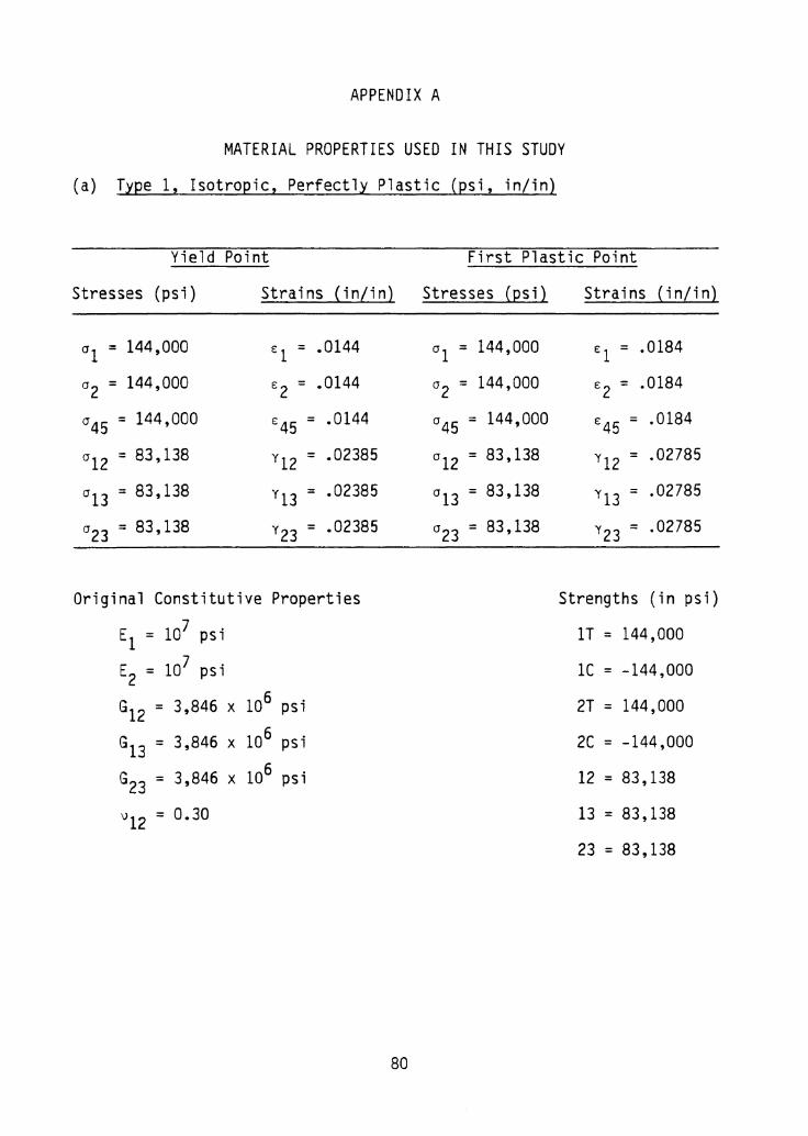
APPENDIX A

MATERIAL PROPERTIES USED IN THIS STUDY

(a) Type 1, Isotropic, Perfectly Plastic (psi, in/in)

Yield Point

Stresses (psi) Strains (inLin)

a1 = 144,000 El = .0144

a2 = 144,000 E = 2 .0144

a45 = 144,000 E45 = .0144

a12 = 83, 138 y12 = .02385

a13 = 83,138 Y13 = .02385

a23 = 83, 138 Y23 = .02385

Original Constitutive Properties

El = 107 psi

E2 = 107 psi

G12 = 3,846 x 106 psi

G13 = 3,846 x 106 psi

G23 = 3,846 x 106 psi

\)12 = 0.30

80

First Plastic Point

Stresses {psi)

al = 144,000

a2 = 144,000

045 = 144,000

012 = 83,138

a13 = 83,138

a23 = 83,138

Strains {in/in}

E 1 = .0184

E = 2 .0184

E45 = .0184

yl2 = .02785

Y13 = .02785

Y23 = .02785

Strengths (in psi)

lT = 144,000

lC = -144,000

2T = 144,000

2C = -144,000

12 = 83,138

13 = 83,138

23 = 83,138

81

{b) Type 2, Boron-Epoxy

Yield Point First Plastic Point

Stresses (psi) Strains {in/in) Stresses (psi) Strains (in/in)

a1 = 120,000 El = .004

a2 = 8,500 E2 = .0031

a45 = 6,600 E45 = .0024

a12 = 5,000 yl2 = .007

a13 = 5,000 Y13 = .007

a23 = 3,571 Y23 = .007

Original Constitutive Properties

E1 = 30 x 106 psi

E2 = 2.7 x 106 psi

G12 = 0.7 x 106 psi

G13 = 0.7 x 106 psi

G23 = 0.5 x 106 psi

\)12 = 0.21

(c) Type 3, Isotrpic II

E = 30 x 106 psi

\) = 0.30

a1 = 160,000

a2 = 20,000

a45 = 10,000

crl2 = 12,800

crl3 = 12,800

a23 = 9,143

El = .0054

E = 2 .0103

E45 = .0034

yl2 = .0221

Y13 = .0221

Y23 = .0221

Strengths (in psi)

lT = 200,000

lC = -200,000

2T = 12,500

2C = -12,500

12 = 19,000

13 = 19,000

23 = 13,800

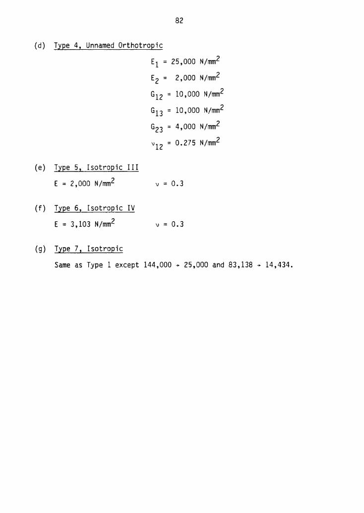
82

(d) Type 4, Unnamed Orthotropic

(e) T,Ype 5 2 Isotropic

E = 2,000 N/mm2

(f) T,Ype 6, Isotropic

E = 3,103 N/mm2

(g) T,Ype 72 Isotropic

III

IV

E1 = 25,000 N/mm2

E2 = 2,000 N/mm2

G12 = 10,000 N/mm2

G13 = 10,000 N/mm2

G23 = 4,000 N/mm2

v12 = 0.275 N/mm2

v = 0.3

v = 0.3

Same as Type 1 except 144,000 + 25,000 and 83,138 + 14,434.

The vita has been removed from the scanned document