1

Geomechanics Notes Robert S. Anderson University of Colorado

Section I - Heat

Table of Contents Chapter Topic Page 1 Introduction 2 2 Radiation – setting the temperature of the planet 5 3 Radiation II – setting the temperature of a one-layer atmosphere 21 4 Radiation III – absorption in translucent materials 25 From Antarctic lakes to coral reefs 5 The heat equation and steady problems: the geotherm 41 6 Radioactivity – bending the geotherm 51 7 Transient problems I – sinusoidal oscillations 62 The snake writhing in an exponential funnel 8 Transient problems II – instantaneous cooling and heating 69 From the grilled cheese sandwich to the age of the earth 9 The lithosphere as a thermal boundary layer 80 10 Advection of heat – temperature profiles in glaciers and orogens 87

total 98

2

Introduction These notes correspond closely to a course I have now taught for about 30 years, called Geomechanics. The course is meant both as a means of teaching the basics of how heat moves about, and how and why fluids move, but as a means of exercising the math and physics that many undergraduates have been exposed to or been made to take in their college career, but have not had the chance to apply to earth science problems. The problems we get to tackle are fundamental, as they touch upon many corners of our science. And they are fun.

Sources The course is inspired by two books, Geodynamics by Turcotte and Schubert, now in its 3rd edition, and by Geoff Davies’ books The Dynamic Earth and its concise and accessible sequel, Mantle Convection for Geologists. I have plucked examples and derivations from these texts, and while I do not attribute the specifics of the derivations in all cases, it should be clear that I have leaned heavily on these works for inspiration. The first edition of Turcotte and Schubert came out while I was in graduate school. I was given the opportunity to read much of it, to dabble in it, as an independent study with Bernard Hallet, for which I am forever grateful. I have also summarized developments of examples taken from the literature and try to give the reader references sufficient to access the original literature when I have done so. And some text has been lifted from other sources of my own, from The Little Book of Geomorphology, and from Suzanne and my book Geomorphology: The Mechancis ands Chemistry of Landscapes.

Strategy I start with how heat moves about because heat is a scalar. It has no direction attached to it. It is not a vector. Something is either hot or cold, not both hot and headed south or cold and going west. This simplifies the math. But the math that we do tangle with in the heat section of the course is useful as a prerequisite for the fluid mechanics that comes in the second portion of the course. The strategy in each of the sections is essentially the same. I start by developing the fundamental equations that represent the physical situation. We start from scratch using the principle of conservation, which in turn informs what physics is required to solve the problem. For example in heat problems, the physics required is representations of how heat is conducted within the medium, and what sources or sinks of heat might occur, say from phase changes or radioactive decay. These master equations are commonly 2nd order partial differential equations (PDEs), which in general can be nasty. Armed with the master equation – of heat or of momentum – we simplify the problem by making assumptions that govern the relative importance of the several terms in the

3

equation. In many cases this transforms our nasty 2nd order partial differential equation to a more easily solved 2nd order ordinary differential equation (an ODE). And then we solve this simpler equation for the problem at hand – in many cases by integrating twice. We will find that the problems differ from one another in what happens at the edges of the space we are considering. These serve as “boundary conditions”, and allow us to solve for the constants of integration that occur when we integrate our differential equations. Examples of boundary conditions include the surface temperature of the ground, or the fact that at a boundary the velocity of a fluid may be taken to be zero. These are things we either can safely assume, or can measure in a given problem. Once we have a final equation, for the temperature profile in heat problems, or the velocity profile in fluid mechanics problems, we may then exercise it. We can calculate the mean temperature or speed. We can calculate the maximum and minimum. Or we can calculate the fluxes that these profiles imply. I write this introduction sitting at my dining room table here in Boulder, Colorado, and am treated to a snowstorm I can watch outside my window. It occurs to me that many of the problems we approach in this course are exemplified by snow. I list a few here, but no doubt there are other connections. • Snow is white, and therefore alters the albedo both locally and on a planet-wide basis. The albedo of the planet oscillates from high in northern latitudes in northern winter to low albedo in the southern latitudes in southern winter. It alters the local radiation budget and distribution of heating on an annual cycle. And the mean albedo of the planet plays a significant role in setting the radiation budget of the planet, and hence the mean annual temperature of the planet. We start there in this course, as all earth scientists should know what sets the surface temperature, and the role of greenhouse gases in altering that temperature. • But snow also settles to the ground at a measurable rate – it looks like about 1 m/s with the flakes of several mm size that are currently falling. We address settling speeds of things in this course – from raindrops in air to crystals in magma to quartz in water. • The thickness of the snowpack alters the flux of heat into and out of the ground beneath it by conduction. Depending on the timing, snow can trap in the cold from early cold snaps, or protect the ground from subsequent cold periods. We spend a significant portion of the heat lectures discussion conduction problems. • It is the pattern of snowfall that governs the pattern of winter mass balance on a glacier. This, along with the summer melt pattern, in turn establishes the pattern of ice flux down a valley required for the glacier to be in equilibrium with the mass balance. We treat the physics of how ice moves down its channel – which in this case is the entire valley – in the fluids portion of this course. • In the course of accumulating, the snow metamorphoses first to firn and then to pure ice with only rare ice bubbles. The process requires diffusion of ice from the tips of the original flakes (high negative curvature) to the crooks of the flakes with high positive curvature. We establish in the heat portion of the course just how diffusion works to alter curvature – as much as Nature abhors a vacuum, She also abhors curvature. • And in lake and glacier ice, as well as in snow, light can penetrate to some degree. These materials are not perfectly opaque. They are translucent. And as the light penetrates, it changes color to leave only blue light at greater depths. We discuss

4

radiation in translucent materials in the first part of the course, addressing say the extinction of light in the ocean that governs the depth profile of photosynthetic (and hence coral) productivity.

References Anderson, R.S., 2008, The Little Book of Geomorphology: Exercising the Principle of

Conservation, 100 pp. Self-published on the web in December 2008 (see http://instaar.colorado.edu/people/robert-s-anderson/misc-detail/)

Anderson, R.S. and S.P. Anderson, 2010, Geomorphology: The Mechanics and Chemistry of Landscapes (Cambridge University Press) textbook, 640 pp., published June 2010.

Davies, G., 1999, Dynamic Earth: Plates, Plumes and Mantle Convection, Cambridge: Cambridge University Press.

Davies, G., 2011, Mantle Convection for Geologists, Cambridge: Cambridge University Press.

Turcotte, D.L. and G. Schubert, 2014, Geodynamics, 3rd edition, Cambridge:

5

Radiation and the Earth’s surface temperature Before we can understand climate change, we need to understand how climate works. We need some background. In particular we need to know what governs the surface temperature of the earth. So what I intend to do in the next few minutes is lay out the physics behind the problem. We’ll see that we must employ some basic physics that we all know about from one or another personal experience. We will assemble those into a story. To anticipate, what we will learn is that in the absence of any atmosphere at all, the earth’s surface will be minus 15°C, or 5°F. Way cold, frozen stiff. We’d live in any ice world. Or maybe not live at all – maybe life would not have evolved at all! So we’ll have to grapple with how the atmosphere does this trick of taking us from the expected -15°C to our present +15°C mean surface temperature. Again to anticipate, it will be those nasty greenhouse gases that actually allow us to be anywhere close to our present temperature. If you learn anything then from this lesson, it should be that these trace greenhouse gases have a lot of leverage on our climate. Ok, the basics. We live on a planet at a certain distance from a star. In fact, we memorized that the sun is 93 million miles away (that is 150 million kilometers). There will be a few other facts about this planet-star system that come into play. Can you think about what they are? Features that come to mind are how big and how hot the sun is, how big and how far from the sun our planet is. And maybe some properties of the planet. Like how white or black it is, and maybe whether or not it has an atmosphere. My task in this lecture is to get us organized and put these pieces together. How does the heat of the star, the Sun, get from the star’s surface to our planet? It is by radiation. This is the one means of transporting heat that can occur through a vacuum. The others, conduction (how heat moves form the coffee in your cup to the outer edge of the cup to warm your hand), and convection (how heat moves by motion of a fluid) cannot happen in deep space. So we must know something about radiation. I like to start with what I call a radiation balance. Consider our planet Earth as a sphere receiving solar radiation. If the planet’s surface is to achieve a constant, steady temperature, the heat it receives from the sun must exactly equal the heat that the earth itself loses to space by radiating. It’s the same thing as a bank account. Your balance is steady (doesn’t change in time) if your income equals your expenses. When we talk about the movement of heat, we use the term heat flux. You have heard about watts, and even perhaps about watts per square meter. A watt is a unit of energy per unit time, joules per second. So watts per square meter is energy per unit area per unit time. We call such things fluxes: something per unit area per unit time. If I now craft more formally my radiation balance, (see Figure 1) I can more specifically say that the energy is balanced if the total energy coming to the earth’s surface per unit time equals the total rate at which it is being lost from the earth’s surface. So we need

6

expressions for both of these, the incoming and the outgoing, each of which will be the product of a flux and an area. Let’s do these one at a time.

Figure 1. Elements of the radiation balance for the Earth. Middle: Earth shown in orbit around Sun, with radii of Sun, Earth and orbit, temperature of the Sun's surface, and the energy flux Qo arriving at the outer edge of the Earth's atmosphere. Top: Inverse - square law for energy flux as a function of distance between source and the object. Bottom: Black body radiation spectra for both Sun and Earth, showing both the dependence of the peak wavelength on surface temperature, and of the total energy emitted (integral beneath the curves). Note logarithmic scale for wavelengths. (after Figure 5.6 A&A 2010) Incoming radiation. The incoming rate of delivery of heat to the planet will simply be the product of the heat flux from the Sun times the area of the earth’s surface that intercepts the solar beam. This product will now have units of energy per unit time, or watts. We call the heat flux from the sun at our distance from the sun the solar constant. It is denoted Qo, and when we want to plug in numbers, its value is 1370 W/m2. (This is not a bad number to memorize.) What about the area we need to multiply by? The relevant area is the area of a circle the radius of the earth, so πR2, where R is the radius of the planet. But there is one more complicating factor: not all of this incoming radiation sticks on the earth. Some bounces, or is said to reflect off the earth. The whiter the earth, the more radiation bounces. We call this bounce factor the albedo of a surface, denoted a. The higher the albedo, the more radiation reflects. Albedo has the same root as albino; it derives from white in Latin for “whiteness”. Or if you are a geologist you might be

7

familiar with albite, a particularly white feldspar. Same root. So if a is the fraction that does not stick, the amount of energy that sticks is 1 minus the albedo. This leaves us with an expression for the incoming radiation that sticks, and that therefore participates in warming up the earth:

Qin = QoπR2 1− a( ) (2.1) But I want to unpack this solar constant a bit. Yes, we can measure it at this distance, but we will want to know how it depends upon some characteristics of the sun and our distance from the sun… We now have to learn a little about how radiation works – and in particular what governs both the flux of heat radiated from a surface and the wavelength of that radiation. It turns out that the heat flux is way sensitive to the temperature of the surface. Our expression for the heat flux from a radiating body is Q =σT 4 (2.2) where σ is a constant called the Stefan-Boltzmann constant, and T is the temperature in Kelvins (absolute temperature). This is called the Stefan-Boltzmann radiation law. Double the temperate and the radiative heat flux goes up by a factor of 24, or 16. This means two things. If we know the temperature of the Sun’s surface, we can calculate the heat flux from the Sun’s surface. And if the temperature of the Sun goes up a little, its radiative output will go up a lot. So the heat flux at the Sun’s surface is Q = σ Ts

4, where Ts is the Sun’s surface temperature. But we are (happily) not at the sun’s surface. We orbit at a distance some 150 million kilometers from the Sun. How do we bridge between the heat flux from at the Sun’s surface and the heat flux at this distance? Here we get to employ another elegant principle of physics. Let’s back into it. Consider for a moment what is between the sun and the earth. This is not a trick question. The answer is pretty much nothing. Certainly nothing that is going to absorb any radiation. The vacuum of space is transparent to radiation. This means that the total amount of radiation passing out across the sun’s surface per second or per year must be the same as the total amount of radiation that passes any sphere at any chosen distance from the sun’s surface in that same unit of time. Otherwise there would be a loss or a gain of energy in between, and we have just argued that there is nothing in between to warm up or to cool off! So we may set up the following little calculation. In words we may state that: The area of sun’s surface times the radiation flux from the sun’s surface = the area of a sphere with radius of the earth’s orbit times the radiation flux across that surface. If we then divide by the surface area of the sphere with our orbit’s radius, we have a formula for the energy flux at our distance from the sun, or the solar constant. Mathematically, this looks like: QsAs = QoAo (2.3)

8

where the s signifies the sun and o the earth’s orbit. Rearranging this we see that

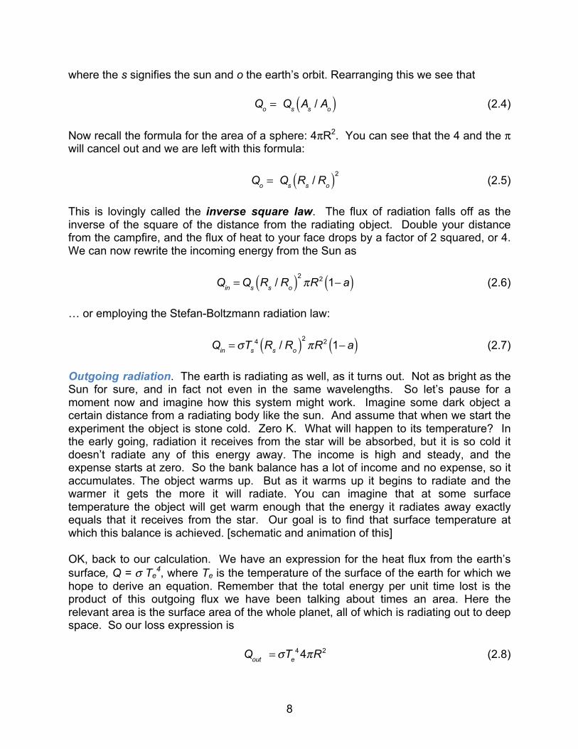
Qo = Qs As / Ao( ) (2.4) Now recall the formula for the area of a sphere: 4πR2. You can see that the 4 and the π will cancel out and we are left with this formula:

Qo = Qs Rs / Ro( )2 (2.5)

This is lovingly called the inverse square law. The flux of radiation falls off as the inverse of the square of the distance from the radiating object. Double your distance from the campfire, and the flux of heat to your face drops by a factor of 2 squared, or 4. We can now rewrite the incoming energy from the Sun as

Qin = Qs Rs / Ro( )2πR2 1− a( ) (2.6)

… or employing the Stefan-Boltzmann radiation law:

Qin =σTs4 Rs / Ro( )2

πR2 1− a( ) (2.7) Outgoing radiation. The earth is radiating as well, as it turns out. Not as bright as the Sun for sure, and in fact not even in the same wavelengths. So let’s pause for a moment now and imagine how this system might work. Imagine some dark object a certain distance from a radiating body like the sun. And assume that when we start the experiment the object is stone cold. Zero K. What will happen to its temperature? In the early going, radiation it receives from the star will be absorbed, but it is so cold it doesn’t radiate any of this energy away. The income is high and steady, and the expense starts at zero. So the bank balance has a lot of income and no expense, so it accumulates. The object warms up. But as it warms up it begins to radiate and the warmer it gets the more it will radiate. You can imagine that at some surface temperature the object will get warm enough that the energy it radiates away exactly equals that it receives from the star. Our goal is to find that surface temperature at which this balance is achieved. [schematic and animation of this] OK, back to our calculation. We have an expression for the heat flux from the earth’s surface, Q = σ Te

4, where Te is the temperature of the surface of the earth for which we hope to derive an equation. Remember that the total energy per unit time lost is the product of this outgoing flux we have been talking about times an area. Here the relevant area is the surface area of the whole planet, all of which is radiating out to deep space. So our loss expression is Qout =σTe

4 4πR2 (2.8)

9

The 4 is there because the surface area of a sphere is 4 times the area of the circle of the same radius. Remember your geometry? We may now set the incoming and outgoing terms equal to one another, and do some algebra to isolate or solve for the surface temperature of the planet: The words: Incoming = outgoing. The math:

QoπR2 1− a( ) =σTe4 4πR2 (2.9)

Notice that the πR2 cancels out. This means that it does not matter how big the planet is (! Can you articulate why that is the case?) Solving for the steady state surface temperature of the planet, we find:

Te = Qo 1− a( ) / 4σ⎡⎣ ⎤⎦

1/4 (2.10)

or if we do not know the solar constant, then more fundamentally:

Te = Qs Rs / Ro( )2

1− a( ) / 4σ⎡⎣⎢

⎤⎦⎥

1/4

(2.11)

Look at this for a moment. [plot of this] Let’s see if it makes sense. As the flux of heat from the star goes up, the temperature of the planet goes up. That makes sense. As the albedo of the planet goes up, the fraction of radiation that sticks, 1-a, goes down, so the temperature of the planet goes down. That makes sense: whiter objects reflect more of the incoming radiation, so receive less heat to warm them up. You can see that as soon as I give you values for Qo, a, and σ, you can calculate the surface temperature T that is required for a balance. I have already said that Qo = 1370W/m2. The Stefan-Boltzmann constant σ is something we can look up in a book: 5.67x10-8 watts m-2 K-4 (Note the progression of 5,6,7,8 that help to memorize this.) But what about this albedo? What is the albedo of our planet? That is a little hard, as dark pieces of the surface are low albedo and light patches are high. A dirt patch here and a puddle of water or a sward of grass and a snow patch… how do we go about documenting or estimating an average?

10

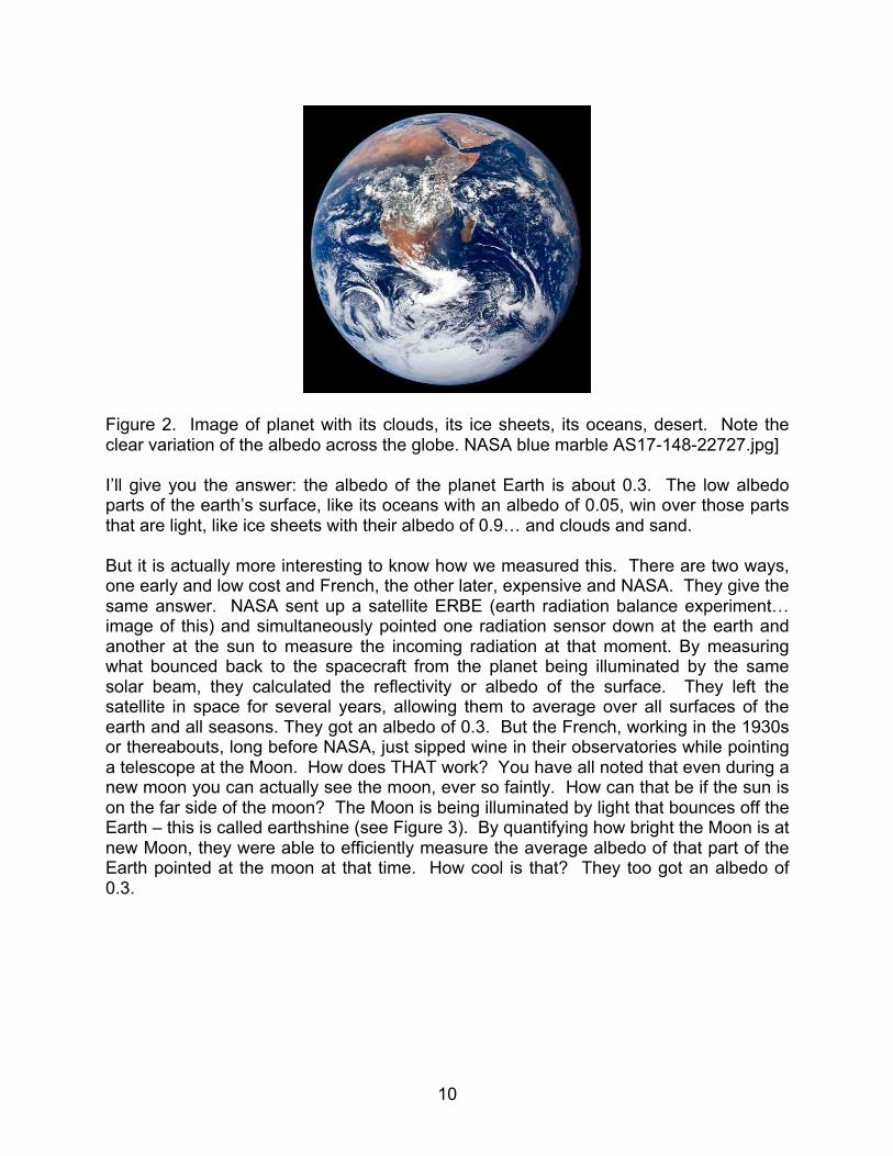
Figure 2. Image of planet with its clouds, its ice sheets, its oceans, desert. Note the clear variation of the albedo across the globe. NASA blue marble AS17-148-22727.jpg] I’ll give you the answer: the albedo of the planet Earth is about 0.3. The low albedo parts of the earth’s surface, like its oceans with an albedo of 0.05, win over those parts that are light, like ice sheets with their albedo of 0.9… and clouds and sand. But it is actually more interesting to know how we measured this. There are two ways, one early and low cost and French, the other later, expensive and NASA. They give the same answer. NASA sent up a satellite ERBE (earth radiation balance experiment… image of this) and simultaneously pointed one radiation sensor down at the earth and another at the sun to measure the incoming radiation at that moment. By measuring what bounced back to the spacecraft from the planet being illuminated by the same solar beam, they calculated the reflectivity or albedo of the surface. They left the satellite in space for several years, allowing them to average over all surfaces of the earth and all seasons. They got an albedo of 0.3. But the French, working in the 1930s or thereabouts, long before NASA, just sipped wine in their observatories while pointing a telescope at the Moon. How does THAT work? You have all noted that even during a new moon you can actually see the moon, ever so faintly. How can that be if the sun is on the far side of the moon? The Moon is being illuminated by light that bounces off the Earth – this is called earthshine (see Figure 3). By quantifying how bright the Moon is at new Moon, they were able to efficiently measure the average albedo of that part of the Earth pointed at the moon at that time. How cool is that? They too got an albedo of 0.3.

11

Figure 3. Earthshine discussed by DaVinci. Credit: Miguel Claro We are finally ready to make the calculation. Using an albedo of 0.3, and the other constants I have noted above, let’s do it first crudely: 1370*0.7 is about 1000, and 5.67 is about 5, and (1000/(4x5x10-8))1/4 = (50x108) 1/4 = 501/4 * 102 = sqrt(7)*100 = 2.64*100 = 264. I had to look up the square root of 7. 264K is -9°C. Doing it more carefully, we find that the surface temperature of the earth should be 258K, or -15°C, or 5°F. Chilly indeed! The whole planet would be locked up in ice. An icehouse world. That is definitely NOT what the surface temperature of our planet Earth is. We sit at about 15°C, plus 15°C. So what did we get wrong? We are off by a whole 30°C. You can see from our equations 10 or 11 that the solar constant would have to be a lot higher than we have measured it, or the albedo of the surface would have to be a lot lower than we have measured it, to achieve this much higher temperature. So, the issue must lie instead in the assumptions or the simplifications we have made. In particular, we have assumed so far that the planet has no atmosphere that might participate in some fashion in the radiation balance. What role can an atmosphere play?

More about radiation: the spectrum

To wrap our heads around this we need to back up and talk a little more about radiation. Recall that I said that temperature not only controls the heat flux, but also the wavelength of the radiation. Take a moment to familiarize yourself with the spectrum of radiation. We have names for a lot of the bands of radiation that should sound familiar:

12

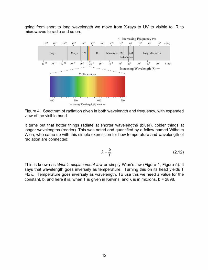
going from short to long wavelength we move from X-rays to UV to visible to IR to microwaves to radio and so on.

Figure 4. Spectrum of radiation given in both wavelength and frequency, with expanded view of the visible band. It turns out that hotter things radiate at shorter wavelengths (bluer), colder things at longer wavelengths (redder). This was noted and quantified by a fellow named Wilhelm Wien, who came up with this simple expression for how temperature and wavelength of radiation are connected:

λ = b

T (2.12)

This is known as Wien’s displacement law or simply Wien’s law (Figure 1; Figure 5). It says that wavelength goes inversely as temperature. Turning this on its head yields T =b/ λ. Temperature goes inversely as wavelength. To use this we need a value for the constant, b, and here it is: when T is given in Kelvins, and λ is in microns, b = 2898.

13

Figure 5. Spectrum of radiation for temperatures ranging from 3000-6000K, showing inverse relation between peak wavelength and surface temperature (dashed line). Wien’s law is really a pretty nifty tool! For example, how do we know how hot the sun is? No astronaut has gone up there with a thermometer and asked the Sun to open wide to put the thermometer under her tongue. But we can stand back here on Earth, point a spectrometer toward the Sun, and measure that its peak radiation is about 0.5 microns. See the graph above. This is in the middle of the visible band, around green. It is not a coincidence that humans have evolved to see in this wavelength band! This means that the temperature of the sun is about 2898/0.5 = 2898*2= 5800K. This is also how we measure the temperatures of other stars in the galaxy. And this is the root of the new thermometers that one uses in hospitals - non-contact thermometers that therefore prevent infections from being passed around. [Bring in such a thermometer.] Note that your skin temperature is around 300K, meaning that the peak radiation from your skin is about 2898/300 = 9-10 microns. This in the infrared (IR), which is why we use IR cameras to detect animals using night vision. Because you are so much cooler than the Sun, you radiate at a much longer wavelength. This also means that we can now rewrite our expression for the surface temperature of the Earth in terms of the Sun’s surface temperature:

Te =Ts

Rs

Ro

⎛

⎝⎜⎞

⎠⎟

1/2 1− a( )4

⎛

⎝⎜

⎞

⎠⎟

1/4

(2.13)

14

The temperature we calculated above for the earth’s surface is about 258K. The Earth would therefore radiate at wavelengths of about 11 microns, again in the IR band. So the incoming radiation from the Sun is centered at 0.5 microns, the outgoing at wavelengths of about 10-11 microns, as seen in the top plot below:

Figure 5. Top: Black body radiation from the Sun and Earth, assuming surface temperatures of 6000K and 255K respectively. Vertical scale is normalized by the peak in each case. Middle: Absorptivity spectra for trace gases in the atmosphere, and bottom: the resulting spectrum of radiation received at Earth’s surface (after Piexoto and Oort, 1994, Figure 6.2) (reproduced from Figure 4.8 in A&A 2010) But before we move on, let me emphasize that we have found out something really quite profound. The planet should be frozen up, an icehouse world, with its mean surface temperature well below 0°C. The measured surface temperature is 30°C above this…so we have done something wrong.

The role of the atmosphere Ok, finally, let’s get back to the role of the atmosphere in our radiation balance. In the interest of time I will simply tell you that the answer lies in the various trace gases that interact with the radiation in specific ways. By “trace” I mean that these gases occur in very small amounts. Remember, our atmosphere is mostly N2 (78%) and O2 (21%) and

15

a little Ar (0.93%), between them making up 99.93% of the atmosphere. That doesn't leave much room for anything else! So all the rest of the gases occur in minute or “trace” amounts. The important players are water vapor H2O, carbon dioxide CO2, methane CH4, and ozone O3. Note that all of these molecules consist of 3-5 atoms, rather than the 1-2 atoms of the major gases of the atmosphere. They are more complicated, and that makes them interact more interestingly with radiation. The bonds between these atoms, as in all molecules, “like” to be a certain length, and given the lengths and strengths of the bonds, and the masses of the atoms involved, they like to vibrate at a certain frequency. When exposed to radiation in this particular frequency band, the bonds get excited and vibrate, and by doing so absorb some of the energy of the radiation in that band. When exposed to radiation in some other band, with higher or lower frequency, they do not get excited, but instead simply allow the radiation to pass by without being absorbed. It is the absorption of radiation in certain wavelengths that alters the radiation balance we have performed. But just how is this radiation being absorbed? I like to think of these molecules doing something of a dance. If you will allow me to anthropomorphize a bit, take the CO2 molecule, which is collinear (the atoms are all lined up in a line – see figure below) and imagine that your head is the carbon, and that your two hands are the two oxygen atoms. Extend your arms out to either side at shoulder height. Now imagine that someone blows a dog whistle in the room. Do you get excited? No, you don’t even hear it! It is at such a high frequency you cannot hear it. But now someone puts on the Rolling Stones or the Grateful Dead or, you choose it, Lady Gaga? You can hear it, and importantly, your body can react at this frequency, given the strengths and the lengths of your muscles, the weights of your hands, and you begin to dance. Given that there are only these two bonds, you can only do several “moves”, each of which might be best done at a certain beat. These trace gases, with their various bond lengths and strengths, do the same thing. So there is a CO2 dance with variations. There is an H2O dance, a methane dance, an ozone dance, and so on. Each dance absorbs energy in a certain frequency (or equivalently, at a certain wavelength) of radiation.

16

Figure 6. Molecular structure of three principal trace gases in Earth’s atmosphere. The vibrational models are noted and the wavelength of absorbtion associated with each are denoted (after Piexoto and Oort, 1992, Figure 6.5, after Houghton, 1965, with permission from American Institute of Physics) (after Figure 5.9 in A&A 2010) Now it so happens that these molecules all get excited by, and therefore absorb energy in, the long wavelength band we call the infrared, or IR. They are completely unexcited by the short wavelength radiation that comes from the Sun, in the visible band, so do not absorb any of the incoming energy. To these molecules, visible radiation is like the dog whistle is to our ears. We see this in a plot of absorption as a function of wavelength, and by comparing the plots for the various molecules you can get some sense of the absorption “portrait” of each molecule. [plot of toothy IR spectrum, smooth SW spectrum] Gases that are “transparent” to incoming shortwave radiation, and absorb in the IR are called greenhouse gases. If you inspect the spectrum of the incoming and outgoing radiation, you can see the bites taken out of the outgoing radiation by the greenhouse gases. Let’s think about the consequences of the absorption in the IR. This absorption of IR constitutes something of a robbery on the outgoing side of our energy balance. Some of the long wavelength energy being emitted by the earth’s surface is being employed by the greenhouse trace gases to drive their little dances, and therefore fails to pass out to space. The earth’s surface must therefore get even warmer (remember, a radiative flux Q ~ T4) in order to radiate enough to balance the incoming radiation, overcoming this robbery of long wavelength radiation as it is transmitted toward space from the earth’s surface.

17

This is the greenhouse effect we have all heard about. And it is huge. The presence of these trace gases in the atmosphere means that the earth is something like 30°C warmer than it would otherwise be in the absence of an atmosphere (with these trace gases). We think that liquid water is a requirement for life. So the bottom line is that greenhouse gases are good in that without them life may not have evolved, or would have only found small refuges in which to exist on or in our planet. But we are also seeing that one can have too much of a good thing. The balance we have been talking about can be tipped by changes in one or another of the climate elements we have been talking about (to be short about it, these are the albedo of the planet, and the trace gas concentrations in the atmosphere.) Before we talk about change, though, at this point we know enough to connect this introductory discussion of climate to another endeavor of humanity – the search for extraterrestrial intelligence SETI. [Figure here or ref to SETI] If life elsewhere indeed obeys the same principles and both physical and chemical requirements as that on Earth, the mean surface temperature of the host planet must be close to the triple point of water, 0°C. One of the requirements for extraterrestrial life is therefore that there be another planet that occupies an orbit at the distance from its star such that its surface temperature is close to 0°C. We call this zone the goldilocks zone: it is not too hot that the water is all vapor, not so cold that it is all frozen, but it is juuuust right.

Figure 7. Goldilocks and the three bowls of porridge.

In the last decade, scientists have been treated to a hunt for planets around other stars, and then a hunt for those planets among them that are in the goldilocks zone. We knew of only a few exoplanets (planets in orbit around a star other than the Sun) before the Kepler experiment launched; the first was confirmed in 1992. [Images of and from Kepler.] The Kepler experiment, in which we trained a huge satellite telescope at a sector of the sky that covers some x% of the dome, and tracked hundreds of thousands of stars for years to watch for hints that they were being orbited by planets. So far we have identified more than 5287 (as of August 2017) exoplanets. And at least a few of these planets are in the goldilocks zone. You now know enough to figure out where that goldilocks zone is, given the star’s temperature (which we get from its color and Wien’s

18

Law), and the measured distance of the planet from its star. Given what we have talked about, you might want to think about what other assumptions go into the calculation of the goldilocks zone!

Figure 8. The sun and our solar system in relation to the Milky Way galaxy. The white circle indicates the area where the majority of exoplanets have been found with current telescopes. Credit: NASA/JPL-Caltech/T. Pyle (from Exoplanet web site)

Drivers of change

Armed with this conceptual and even quantitative picture of what governs the surface temperature of this or any other planet, we can begin to explore how various bits of the physics could potentially change through time – both in the deeper geological past and in the future, assisted by humans. We can list the potential culprits behind change: • Variation in the sun’s radiative output • Variation in the earth’s albedo • Variation in the distance to the sun • Variation in the trace gas content of the atmosphere

changes in the sun’s temperature Sun spot cycle. But this is only 0.1% change on 11-year cycle.

19

Faint young sun paradox. Why is this a paradox? Young stars are thought to emit less radiation, be cooler. Yet the early Earth still has evidence of liquid water at the surface during this less luminous phase. The Stefan-Boltzmann law connects Tsun to Q… then use inverse square law to get Qo, and then on to the surface temperature of the planet. You will find that an even larger greenhouse effect is required in order to counter the less luminous Sun. And now a wrinkle in this: young stars are very flare-y, and these flares could have driven space weather that produced nitrous oxides capable of warming the planet, and organic molecules from inorganic molecules, driving evolution of life, basically a monster global Urey Miller experiment… (see Eos July 2016 and NatGeo article on which the report is based)

changes in the earth’s albedo clouds deserts/vegetation ice and ocean (more ice with high albedo goes hand in hand with less ocean with low albedo, so ice ages have a double whammy impact) triggered snowball earth times are important pre-600Ma albedo feedback summary does albedo of the planet change when land plants evolve?

changes in the distance to the sun not in the mean but the orbit is eccentric and it changes. 1% to 4% on 100 ka cycles. Does this matter to the annually averaged radiation delivered to the earth surface?

changes in the trace gases Long term evolution of the atmosphere Short term changes as seen in ice record archive of atmospheric gas Human additions nailed down using 14C in CO2

Summary

To summarize, let me list what pieces of physics we have employed, and what facts we need to know to be quantitative about a planet’s mean annual surface temperature:

Physics we need to know Radiation balance Stefan-Boltzmann radiation law Wien’s law Inverse square law Albedo Absorption of radiation by molecules

20

Facts we need to know Radius of Earth’s orbit Radius of the Sun Albedo of the planet Stefan-Boltzmann constant Constant in Wien’s Law Wavelength of peak radiation from the Sun

Geometry we need to know Area of a circle Surface area of a sphere

Challenge II

What is the minimal explanation needed? Here is our system: One star with prescribed radius and temperature One planet with known distance from star, known radius, and surface temperature to be calculated The problem: Given a radiation law relating heat flux to surface temperature, calculate the surface temperature of the planet required to balance the input of energy from the star. You will have to craft a radiation energy balance for the planet You will have to figure out how to relate the surface radiation flux from the star to the flux at any other distance from the star. This nicely sets up the problem of evaluating the “goldilocks distance” for any planet orbiting any other star.

References A&A: Anderson, R.S. and S.P. Anderson, 2010, Geomorphology: The Mechanics and

Chemistry of Landscapes (Cambridge University Press) textbook, 640 pp., published June 2010.

21

Radiation II - The one-layer atmosphere We have now seen that the surface temperature of our planet in the absence of an atmosphere should be about -15°C. We have also discussed the essence of greenhouse gases, how they work to absorb energy especially in the IR. We have said that they must be responsible for warming the surface of the earth from the -15°C we expect in the absence of an atmosphere to its present level of about +15°C. I note here that a good candidate for the no-atmosphere calculation is the Moon … although the rate of rotation of the Moon may mean that one side is illuminated for a long time, and therefore experiences large temperature swings… Langley did calculations of this sort in 1890… While we have acknowledged that the atmosphere and in particular its trace gases significantly raise the temperature of the surface of the planet, we have calculated how warm the atmosphere ought to be. This is the goal of this lecture.

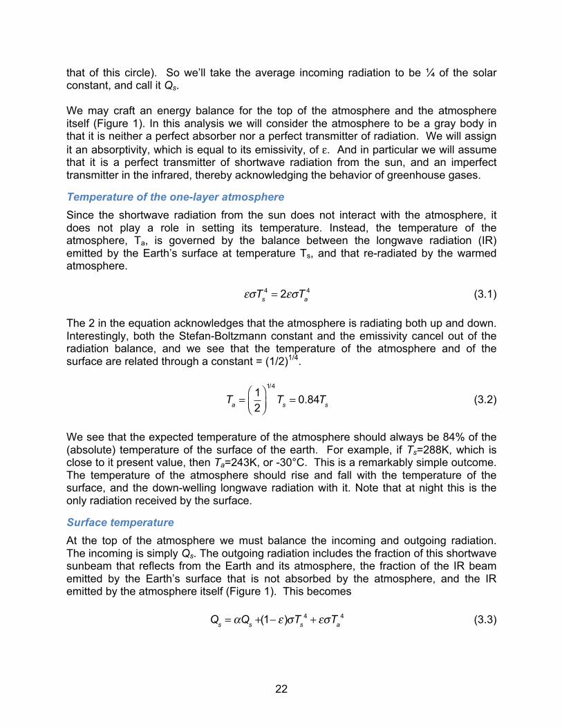
Figure 1. Schematic diagram of the one-layer atmosphere (gray) over the surface of the earth. Consider the simplest possible atmosphere, one in which the properties are uniform throughout and that lies between Earth’s surface and outer space. Our calculation is dubbed the one-layer atmosphere model for that reason. Let us assemble the constraints on this calculation. As always, we will assume that the system is in radiative equilibrium. The energy arriving from the sun must be balanced by the energy leaving the earth. Another way to take into account the different geometry of arrival vs. loss of energy is to employ the ratio of the surface area over which the sunlight is collected (the area of a circle the size of the planet) to the surface area of the planet (which is 4 times

22

that of this circle). So we’ll take the average incoming radiation to be ¼ of the solar constant, and call it Qs. We may craft an energy balance for the top of the atmosphere and the atmosphere itself (Figure 1). In this analysis we will consider the atmosphere to be a gray body in that it is neither a perfect absorber nor a perfect transmitter of radiation. We will assign it an absorptivity, which is equal to its emissivity, of ε. And in particular we will assume that it is a perfect transmitter of shortwave radiation from the sun, and an imperfect transmitter in the infrared, thereby acknowledging the behavior of greenhouse gases.

Temperature of the one-layer atmosphere Since the shortwave radiation from the sun does not interact with the atmosphere, it does not play a role in setting its temperature. Instead, the temperature of the atmosphere, Ta, is governed by the balance between the longwave radiation (IR) emitted by the Earth’s surface at temperature Ts, and that re-radiated by the warmed atmosphere. εσTs

4 = 2εσTa4 (3.1)

The 2 in the equation acknowledges that the atmosphere is radiating both up and down. Interestingly, both the Stefan-Boltzmann constant and the emissivity cancel out of the radiation balance, and we see that the temperature of the atmosphere and of the surface are related through a constant = (1/2)1/4.

Ta =12

⎛⎝⎜

⎞⎠⎟

1/4

Ts = 0.84Ts (3.2)

We see that the expected temperature of the atmosphere should always be 84% of the (absolute) temperature of the surface of the earth. For example, if Ts=288K, which is close to it present value, then Ta=243K, or -30°C. This is a remarkably simple outcome. The temperature of the atmosphere should rise and fall with the temperature of the surface, and the down-welling longwave radiation with it. Note that at night this is the only radiation received by the surface.

Surface temperature At the top of the atmosphere we must balance the incoming and outgoing radiation. The incoming is simply Qs. The outgoing radiation includes the fraction of this shortwave sunbeam that reflects from the Earth and its atmosphere, the fraction of the IR beam emitted by the Earth’s surface that is not absorbed by the atmosphere, and the IR emitted by the atmosphere itself (Figure 1). This becomes Qs = αQs +(1− ε)σTs

4 + εσTa4 (3.3)

23

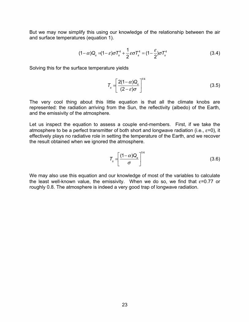
But we may now simplify this using our knowledge of the relationship between the air and surface temperatures (equation 1).

(1−α )Qs =(1− ε)σTs4 + 12εσTs

4 = (1− ε2)σTs

4 (3.4)

Solving this for the surface temperature yields

Ts =2(1−α )Qs

(2 − ε)σ⎡

⎣⎢

⎤

⎦⎥

1/4

(3.5)

The very cool thing about this little equation is that all the climate knobs are represented: the radiation arriving from the Sun, the reflectivity (albedo) of the Earth, and the emissivity of the atmosphere. Let us inspect the equation to assess a couple end-members. First, if we take the atmosphere to be a perfect transmitter of both short and longwave radiation (i.e., ε=0), it effectively plays no radiative role in setting the temperature of the Earth, and we recover the result obtained when we ignored the atmosphere.

Ts =(1−α )Qs

σ⎡

⎣⎢

⎤

⎦⎥

1/4

(3.6)

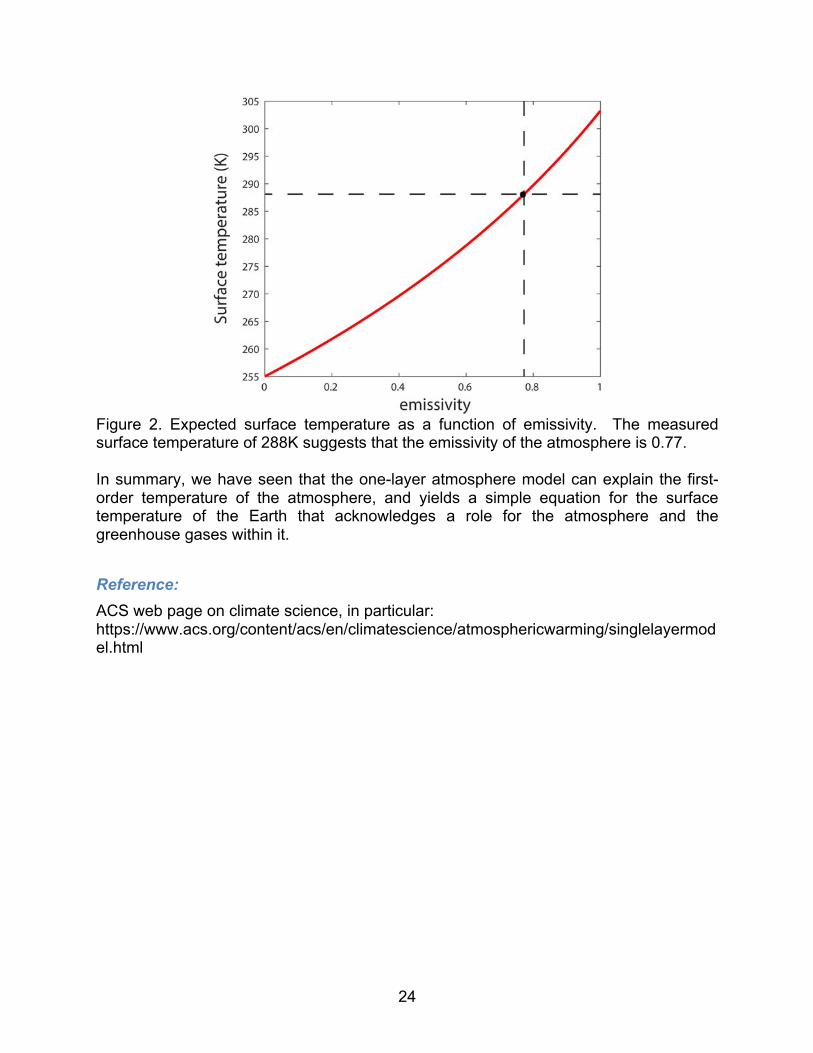
We may also use this equation and our knowledge of most of the variables to calculate the least well-known value, the emissivity. When we do so, we find that ε=0.77 or roughly 0.8. The atmosphere is indeed a very good trap of longwave radiation.

24

Figure 2. Expected surface temperature as a function of emissivity. The measured surface temperature of 288K suggests that the emissivity of the atmosphere is 0.77. In summary, we have seen that the one-layer atmosphere model can explain the first-order temperature of the atmosphere, and yields a simple equation for the surface temperature of the Earth that acknowledges a role for the atmosphere and the greenhouse gases within it.

Reference: ACS web page on climate science, in particular: https://www.acs.org/content/acs/en/climatescience/atmosphericwarming/singlelayermodel.html

25

Radiation III: Absorption within translucent materials Introduction We have seen how a radiation balance governs the mean annual surface temperature of our planet. We have seen how the presence of an atmosphere containing greenhouse gases alters this balance, allowing the surface temperature to be 30°C warmer. And we have calculated the expected mean temperature of a one-layer atmosphere. Here we tangle more directly with how radiation interacts with a medium that is neither perfectly reflective, nor perfectly opaque (like rock). Such materials are called translucent. They absorb some fraction of the radiation as it passes through, leaving less that travels yet further into the medium. Early studies of this system include Bouguer. Beer, and later Lambert, formalized the mathematical treatment of the attenuation of radiation. We now derive what is called Beer’s law, also known as the Beer-Lambert, or the Beer-Lambert-Bouguer law. We then apply that law to problems that include: the color of water, the extinction of light in the ocean and its relevance to the rate of coral growth, the thickness of ice on permanently frozen Antarctic lakes and the temperature profiles in the ice; and the expected profile with elevation of the rate of production of cosmogenic radionuclides. In the course of this discussion we will become familiar with the following terms: Scattering Transmittance Absorbance Attenuation factor Attenuation length scale Optical depth

Derivation of the Beer-Lambert Law Consider a material receiving light or radiation at a flux of Io, in units of watts/m2, or J/m2/s. For materials of uniform radiative properties, the rate of change of radiative flux, I, with depth, z, depends upon the product of an attenuation factor with the flux of radiation received at that position (Figure 0). Hence

dIdz

= −µI (4.1)

26

Figure 1. Illustration of the Beer-Lambert Law. Incoming radiation, Io, is attenuated through the medium at a rate governed by the attenuation coefficient µ. The radiation lost is equivalent to the heat energy gained by the material. This should look familiar as it has the same basic form as the equation for radioactive decay. This first order ordinary differential equation (ODE) may be solved by appeal to the boundary condition that at the surface, z=0, the radiative flux is Io. Separating variables yields

dII= −µdz (4.2)

Integrating both sides gives ln(I) = −µz +C (4.3) where C is a constant of integration. Appealing to the boundary condition suggests C = ln(Io ) (4.4) Making use of the property of logarithms that lnA - lnB = ln(A/B) then allows us to write

27

ln I

Io

⎡

⎣⎢

⎤

⎦⎥ = −µz (4.5)

Taking the anti-log of, or exponentiating, both sides reveals the final solution to the ODE: I = Ioe

−µz (4.6) The flux of radiation exponentially declines with depth at a rate governed by the attenuation factor (Figure 0). Again, recall that we have assumed the material properties are uniform. The transmittance of a material is defined as the ratio of radiation at some depth to that at the surface. The transmittance is therefore simply

T = I(z)

I0

= e−µz = e−τ (4.7)

where Io is the incident radiation at the surface of the material, µ is the extinction coefficient or attenuation factor (m-1), and z is depth into the material. Here τ is called the optical depth. The greater the optical depth, the less radiation is transmitted to the depth z. It is also convenient and perhaps more intuitive to define a characteristic e-folding attenuation depth, 1/k, at which the transmittance is 1/e of that at the surface. In many problems, such as oceanic light penetration, it is useful to define the depth at which the transmittance falls to 1% of that at the surface. This corresponds to 4.6τ; in the ocean this depth corresponds to the base of the photic zone. Where does all this radiation go? Energy does not simply disappear. It has been absorbed, randomized, and can now be considered a source of heat. We can obtain the absorption as a function of depth directly from the ODE in equation 1. It is merely the opposite sign of the rate of attenuation (Figure 0): A = µI = µIoe

−µz (4.8) Note that the dimensions of the absorption are carried in µI, which are now energy per unit volume per unit time, or W/m3. We now explore problems in which the profile of radiation, or the profile of heat production, are important.

The color of water It turns out that the attenuation of light depends upon the wavelength of that light and the molecular make-up of the material through which it is passing. Absorption of light in water is accomplished largely through the excitation of vibrational modes in the water

28

molecules, which are preferentially excited by red light. As the red light is absorbed, the remaining spectrum becomes bluer. The longer the path of the light through the water, the bluer the remaining light. One sees this in swimming pools, the deep end being bluer than the shallow, and even shallow pools are bluer than the water in a small bowl (which looks clear). Ocean or lake divers experience this; the light a few to a few tens of meters below the surface is distinctly bluer than the incident sunlight. Note that this is a different phenomenon altogether than that explaining the blue color of sky. Sky is blue because blue light preferentially scatters in air. The beam coming directly from the sun has the blue light scattered away from it, leaving it redder or yellower. The rest of the atmosphere looks blue because the only light we receive from it is the light scattered to your eye from the atmosphere, and it is preferentially blue (see Bohren, 2001).

Coral growth problem All models of carbonate platform evolution, or coral reef evolution must capture the essence of the growth rate of corals. These organisms are photosynthetic, and hence depend upon the amount of photosynthetically available radiation (also called PAR) as a function of position within the water column. One must marry algorithms for light extinction in the water column (physics), and for response of the coral to that light (biology). To capture the former we employ the Beer-Lambert Law, which collapses to I = Ioe

−kz (4.9) where z is depth into the water column, Io is the incident radiative flux in the visible range (hence available for photosynthesis), and k is the extinction coefficient (Figure 4). The latter ranges from 0.04 – 0.16 m-1 in seawater. This corresponds to characteristic penetration e-folding attenuation depths (1/k) of 7-20 m. Importantly, this extinction coefficient varies significantly with the particulate concentration in the water column. Hence light is much more rapidly extinguished with depth (high k) in the near-shore environment than on the shelf edge. The biological component of the growth rate is calculated from an empirically derived function based upon measured coral growth rates G = Gmax tanh(I / Isat ) (4.10) where Isat is a saturating radiation intensity that sets the shape of the growth rate curve, and Gmax is the maximum growth rate that the particular species is capable of achieving (e.g., Bosschler and Schlager, 1992) (Figure 4).

29

Figure 2. Radiation extinction profile and associated coral growth rate profile. Isat = 200; Io = 2100; k = 0.12 m-1; Gmax = 1 cm/yr. One may add complexity to this by explicitly acknowledging the tidal cycle (e.g., Toomey et al., 213). In addition, one may treat the roles of water temperature (K.D. Anderson et al., 2017), and the turbidity of the water, both of which will vary spatially, and will change on climate time scales. Armed with this coral growth algorithm, one may model the resulting evolution of coral reefs using a time series of relative sea level. This demands knowledge of the global sealevel history, as well as the local tectonic setting that governs the rock uplift pattern. I refer the reader here to early work by Galewsky (1998), and for more recent work by Toomey et al. (2013). Dependence on depth and hence light attenuation (uniform properties) Role of suspended particles that will reduce transmission And appeal to this as a means of damping coral growth near landmass (hence favoring barrier reefs over coral fringe)

Temperature of a lake On the North Slope of Alaska, and elsewhere in the Arctic, there are many lakes (e.g., Figure 3). Most of these are shallow, a few meters deep. And they are very important as sites of summer breeding grounds for many species of birds. While these freeze over in the winter, they have open water for the summer months. Here we ask what the lake temperatures might be in the summer. The simplest question to ask is what mean (time-averaged) temperature might be attained. A more difficult question would be what the day-night amplitude of the change might be.

30

Figure 3. A typical scene on the north slope of Alaska, here near Drew Point. These lakes are a few meters deep, and dot a landscape that is otherwise very flat. (RSA photo) Consider the thermal problem summarized in Figure 4. We first must craft a conservation of heat equation for a lake of depth H. We will assume that the sources of heat are shortwave radiation from the Sun, longwave radiation from the atmosphere, and geothermal heat from the Earth. The loss of heat we will assume is simply longwave radiation from its top surface. I acknowledge that the full energy balance is more complicated, but I argue that we can get a long way toward the answer with these simple assumptions.

31

Figure 4. Schematic diagram for the temperature of a shallow lake of area A and depth H. The energy balance is therefore:

∂(ρcTLAH)∂t

= I(1− a)A+σTA4A−σTL

4A+QGA (4.11)

Here T is temperature in Kelvins, subscripts L and A correspond to lake and atmosphere, respectively, A is lake area, H lake depth, σ is the Stefan-Boltzmann constant, I the shortwave solar radiation flux, a the albedo of the lake, and QG the geothermal energy flux. This looks pretty complicated, but let’s take some steps to simplify. One can see immediately that the area of the lake cancels from all terms. I will also assume that the geothermal flux is trivial compared to the energy delivered from the Sun. How can I simply assert this? It is worth knowing some values. Typical values of geothermal flux are tens of milliwatts per square meter, whereas typical values of solar flux, even at these high latitudes, are hundreds of watts per square meter. Remember the solar constant is 1370 W/m2. They are five orders of magnitude different… so we may safely neglect the role of geothermal heat (at least in the summer months…). That gets rid of the last term. In fact, if we stick to the simpler question of what sets the mean (temporally averaged) temperature of the lake, and not get tangled up in its change over the course of a day or a year, then we may even drop the whole left hand side and set it to zero. Well that is pretty cool, because it changes the problem from a differential equation (college problem) to an algebraic equation (middle school problem). We can do this. Now solve the remaining equation for the expected mean temperature of the lake, TL:

32

TL =

I(1− a)σ

+TA4⎡

⎣⎢

⎤

⎦⎥

1/4

(4.12)

Remember the answer will be in Kelvins. Does this make sense? Dimensions check out (do this yourself; it is always the first thing to do once you have what you think is an answer!). The lake temperature increases as the solar radiation increases, and as the lake albedo decreases. And it increases as the temperature of the atmosphere above it increases. Let’s plug in some reasonable numbers. Let I=200 Wm-2, a=0.05, σ=5.67x10-8 Wm-2K-4. But what about the atmosphere? We need its temperature. That is indeed hard to come by, but remember our one-layer atmosphere calculation? That is a place to start. Given that we are far north, let’s use a lower value, like TA=-40°C = 243K. I calculate that the time-averaged lake temperature is TL=282K, or about 9°C. Once again, working this simple problem arms us with a very efficient way to assess the roles of the various elements of the problem. We can ask what will change from place to place (I), and what will change with time as climate changes (TA, and perhaps a), and we can see how sensitive the system is to these changes. We can wait to ask more formally the more complicated question of how the temperature of the lake will change over the course of a day as the solar radiation varies. But just by inspection of equation 11, we can evaluate the role of the lake depth, H. As the lake depth, and the water density and heat capacity will not change over the course of a day, we may take them out of the time derivative and divide all terms by them. That will leave on the left hand side simply the rate of change of temperature, dT/dt, and on the right hand side all terms will have a (1/H) in front of them. This alone tells us that the rate of change of the lake temperature is inversely dependent on the lake depth. The shallower the lake, the more rapidly its temperature will change, and hence the more its temperature will change over the course of a day.

Cosmogenic radionuclide production This attention to how radiation is attenuated in a medium is also relevant to the emerging tool of cosmogenic radionuclides in geomorphology. We now commonly employ cosmogenic radionuclides like 10Be and 26Al to obtain ages of geomorphic features, and to calculate long-term erosion rates. In all such methods, we require knowledge of the production rate of cosmogenic radionuclides at the surface of the earth. Production of radionuclides in rock at the surface of the Earth requires passage of the beam of cosmic radiation through the atmosphere. As any other radiation, it is attenuated as it passes through the medium, at a rate that is governed by the mass it encounters along its path. This is captured by a version of the Beer-Lambert Law with a “mass attenuation” factor, Λ. The production rate falls off with distance downward into

33

the atmosphere. Taking elevation to be positive upward, production will increase with elevation toward the maximum rate one would encounter in outer space. We wish to derive a simple model of this production as a function of elevation.

SlabatmosphereThe simplest model is one in which we treat the atmosphere as being uniform in density, ρ, with a fixed thickness, H. For example, take the density to be that at sealevel, and calculate the height of atmosphere of that density required to generate the sea level atmospheric pressure. Since in a uniform density material P=ρgH, we can calculate this so-called scale height of the atmosphere to be H=Psl/gρ. For Psl=105 Pa, and ρ=1.22 kg/m3, this yields H=8364 m or 8.4 km. Attenuation of production rate with depth into this slab atmosphere is simply P = PH e

−(ρ(H−z)/Λ) (4.13) where PH is the production rate at the top of the atmosphere. The attenuation length, which is the inverse of the attenuation factor, is simply Λ/ρ; I sometimes denote this as z*, to acknowledge that it is a length scale. In reality we have better constraint on the production rate at sealevel rather than that in outer space (or the top of the atmosphere), hence use instead P = Psl e

(ρz/Λ) (4.14) For heights greater than H we assume the radiation is unchanging: P(z>H) =P(H). This is plotted in Figure 5. The production rate increases exponentially with elevation z. The effective e-folding length scale for the cosmogenic radionuclide production rate in the atmosphere is z* = Λ/ρ = 1300 m, or a little more than a kilometer. Note that the production rate at the top of the atmosphere, here taken to be 8 km, is of the order of 4000, while that at sealevel is about 6 atoms/gr-qtz-year. This three-orders-of-magnitude increase reveals the expected high levels of radiation one would encounter in outer scape – and indeed this is of great concern for space travel.

34

Figure 5. Profile of CRN production calculated for two cases. black dashed: slab atmosphere with uniform density and thickness 8.4 km; red: exponentially declining atmospheric density. [exercise for the reader: calculate the expected radiation at the height at which most airliners travel. Pilots and airline staff experience high doses at these elevations.] We will see that while this simple model breaks down at alpine elevations, it holds well for low elevations, and hence the scaling height of 1300 m is a useful and simple rule of thumb. For z=1300 m, P=Psl*e=6*2.7=16, while at z=2*1300m=2600m, P=Psl*a2=6*7.4=44 at/gr-qtz-yr. By elevations of 2600 m=8500 ft, the production rate is expected to be more than 7-fold greater than at sealevel.

AtmospherewithanexponentialdensityprofileIn the above simple model we have neglected the reality that the atmosphere is a gas whose density decreases with elevation. Think about how this should affect our simple slab model. This requires revisiting Beer’s Law. Our mass attenuation factor ρ/Λ now becomes a function of position because density ρ declines with z:

I = Io e− ρ (z)

Λ0

ℓ

∫ dz (4.15)

The attenuation factor is no longer uniform, and we must integrate the attenuation along the path l. In our case this translates into the need to integrate along the density profile in the atmosphere. Consider an atmosphere in which the density declines exponentially with elevation (this is an approximation that neglects the thermal structure of the atmosphere, but again is a good place to start). The density profile is then

35

ρ = ρsle

−z/h (4.16) where h is now the characteristic length scale for decline of density. In our atmosphere h=8.4 km. Acknowledging that z is taken positive upward, which is the opposite direction of the passage of the radiation, the proper form of the Beer-Lambert Law becomes

P = Po e−

ρsle− z/h

Λz

∞

∫ dz (4.17)

To evaluate the production at any elevation z, we must integrate the attenuation over the height z to infinity. Performing this integral yields

P = Po e−ρslhΛe− z/h

(4.18) Checking this, we see that at z=infinity, P=Po, as required. We plot the resulting profile of production in Figure 5, along with the simpler slab case. In both cases the farfield (outer space) value of the production rate is equivalent. Why? Because in both cases we require that the production rate at sealevel be that we measure, and in each case the total mass of the atmosphere is the same, hence the total attenuation of the radiation beam is equivalent. But in the more realistic non-uniform atmosphere, the production rate declines only trivially in the outer atmosphere where the air is so rarified, and then declines more rapidly at lower elevations. As the two curves separate significantly by about 2 km elevation, it is more appropriate to use the declining density profile case in estimating the radionuclide production rate at elevations above say 1 km.

TopographicshieldingAnother requirement in the cosmogenic world is calculation of the role of topographic setting in masking some portion of the cosmic radiation that can generate production of radionuclides. You might imagine that if you are sampling from a rock surface deep in a narrow canyon, that some fraction of the cosmic beam would be masked by the surrounding canyon walls. The calculation requires that we know the fraction of the flux from any particular direction that will be masked by a horizon of a measured height. We commonly document the angle of the horizon in a number (8 or more) directions from a sampling site, and then calculate the total blocking. We report a number between 0 and 1, 1 being no blocking, 0 being total blocking of the cosmic flux and hence production. We must therefore know the cosmic flux as a function of zenith angle (θ, defined as angle from vertical (the zenith)) (Figure 8). The dependence commonly employed in this calculation is a power law of the sin function, in particular sin2.3 (see for example Balco; Gosse and Phillips).

36

Here I ask what pattern we would expect if we start from first principles. Consider that the incoming radiation is isotropic, meaning that it is evenly distributed with angle at the top of the atmosphere. To be clear, this means that for a given position on the globe, the strength of the incoming radiative beam that could potentially produce radionuclides is uniformly distributed with respect to horizontal and vertical angle at the top of the atmosphere. The beam has nothing to do with the sun. The relevant beam, that with enough energy to generate the nuclear reactions from which these nuclides are comes not from the sun but from supernovae in the galaxy... and these are assumed to be evenly distributed over the sky dome. Ok, now consider a beam coming from some zenith angle θ (Figure 6). Given that the atmosphere has a finite thickness, the beam will pass through greater lengths of atmosphere as this angle increases. And given that the greater the length of the path through the atmosphere, the exponentially lower the production (as we have already seen above), one would expect that the production associated with beams far from the vertical will be dramatically lower. That is our expectation. But here we want to be quantitative about it so that we can do the proper calculation of the topographic shielding.

Figure 6. Schematic diagram for calculation of beam lengths through a slab atmosphere of uniform density. A) Flat Earth. B) Spherical Earth. θ=zenith angle. Io is beam intensity (W/m2) at the top of the atmosphere. H is atmospheric thickness, L beam length, and Lmax maximum length of beam in spherical earth case. We proceed incrementally. Let us start with the simplest calculation, as always. Consider therefore a slab atmosphere of uniform density... and a flat Earth (Figure 6A). Whoa, you say, how heretical of you Bob. Bear with me. It is still an appropriate place to start. In this case, the length of the beam, L, is related very simply to the zenith angle: L = H/cos(θ), where again H is the thickness of the slab atmosphere. We can then evaluate the effective strength of the beam and hence its ability to produce radionuclides as a function of L and hence θ. The intensity of the incoming cosmic beam at the surface is therefore simply I = Ioe

−ρH /Λcosθ (4.19)

37

This is a maximum when θ=0°, i.e., for the beam that is exactly vertical, is zero for the horizontal beam (θ=90°), and should smoothly decline from one the other. We show this pattern in Figure 7, normalized by the maximum, along with the empirically determined sin2.3 curve.

Figure 7. Ratio of radiation intensity for beams of full range of zenith angles. Green: slab atmosphere, flat Earth case. Black dashed: sin2.3 pattern. Red dashed: slab atmosphere but incorporates a curved Earth. While this appears to have the appropriate behavior, it only broadly mimics the curve used in most studies. Why the difference? We have two assumptions to revisit: 1) the Earth is in fact spherical (!), and 2) the density of the atmosphere declines with elevation. Do either of these two features of the atmosphere account for the difference?

Slabatmosphere,sphericalEarthFirst we move from the flat Earth to the spherical Earth, with radius R. From Figure 6B one can see that this will certainly impact the expected path lengths, especially for nearly horizontal beams. Even the perfectly horizontal beam is now finite in length, with length Lmax, rather than infinite. The essence of the problem is entirely geometric. We require a formula for the path length of the beam through the uniform atmosphere, and can then enact Beer’s law. But the path length formula is not trivial. Working some geometry, and employing the law of sines (A/sin(a) = B/sin(b) = C/sin(c), where the side A is opposite the angle a, etc.), results in the following formula for the path length:

L = R +H

sin(180 −θ)sin θ − asin R

R +Hsin(180 −θ)

⎛⎝⎜

⎞⎠⎟

⎡

⎣⎢

⎤

⎦⎥ (4.20)

The maximum length, that when θ=90°, is then

38

Lmax = R +H( )cos arcsin

RR +H

⎛⎝⎜

⎞⎠⎟

⎡

⎣⎢

⎤

⎦⎥ = R tan arccos

RR +H

⎛⎝⎜

⎞⎠⎟

⎡

⎣⎢

⎤

⎦⎥ (4.21)

Prove to yourself that these two expressions are equivalent using the diagram of Figure 6. Given these path lengths as a function of zenith angle, we can assess the attenuation of the beam using Beers Law. Again normalizing with respect to the shortest path (zenith angle = 0; L=H), we plot this in Figure 7 as the red dashed curve. At this scale, the pattern looks identical to that for the flat Earth case. The change in the pattern is trivial. This is largely because all the change occurs at high zenith angles (beams close to the horizon), as shown in Figure 8.

Figure 8. Path length for radiation traveling through atmosphere over the full range of possible zenith angles (θ=0 signifies vertical beam). A horizontal beam (zenith angle = 90°) in the flat Earth case yields infinite length, whereas a horizontal beam on spherical Earth with slab atmosphere 8.4 km thick has a path length of 322 km. Much to our dismay, we have not solved the problem. We are no closer to the sin2.3

pattern used by the cosmogenic radionuclide community. The next assumption we must revisit is that of uniform density. Here I give up (get lazy) and resort to a numerical calculation. I shoot rays in from different zenith angles, assess the density at each point along the path, calculate the attenuation rate, and update the remaining beam strength. There is one little trick required, however. At any point along a beam path, one must calculate the local height above the surface, z, which governs the local density of the atmosphere. I appeal to the law of cosines to calculate the distance from the center of the Earth (R + z)2 = R2 + L2 − 2RLcos(180 −θ) (4.22) where L is the distance from the point on the surface of the Earth along the beam. This results in the following formula for the local height above the surface:

39

z = R2 + L2 − 2RLcos(180 −θ) −R (4.23) The change in the beam strength is then dI = −(ρ(z) / Λ)IdL (4.24) where I is the beam strength entering this little element dL, and ρ(z) is the local density, which we calculate form the exponentially declining density structure. The pattern of the beam strength remaining at the surface of the Earth is shown in Figure 7. As it turns out, this too results in a profile that is essentially indistinguishable from that with a slab atmosphere. Given the assumptions I have made in the above analysis, I am still (sadly) unable to explain why the empirical pattern (black dashed line in Figure 7) is used. I hasten to say that this should not in any way reduce confidence in the use of the empirical rule – it simply means that there is other physics involved that my simple model does not capture.

Summary We have exercised several applications of how radiation matters in geologic and geomorphic systems. In all of these cases radiation can penetrate into translucent medium (the atmosphere, water, ice), and we can employ the Beer-Lambert Law to calculate the attenuation of the beam. We have seen how that penetration can result in heating of the medium. We have seen how the attenuation of the beam plays a role in extinction of life-driving light in the water column, and governs the elevation pattern of production of radionuclides in rock surfaces. And by addressing the dependence of extinction on wavelength of the light in water, we can even explain why deep water is blue. In the course of this chapter we have employed the following principles and rules from physics and math:

Beer-Lambert Law Conservation of heat Energy associated with phase change Law of sines Law of cosines Integration

References Anderson, K.D., N.E. Cantin, S.F. Heron, C. Pisapia and M.S. Pratchett, 2017, Variation

in growth rates of branching corals along Australia’s Great Barrier Reef, Scientific Reports 7: 2920, doi:10.1038/s41598-017-03085-1.

Bohren, C., 2001, Clouds in a Glass of Beer, Dover, 224 pp.

40

Bosschler, H. and Schlager, W., 1992, Computer simulation of reef growth, Sedimentology 39: 503-512.

Galewsky, J., 1998, The dynamics of foreland basin carbonate platforms: tectonic and

eustatic controls. Basin Research 10 (4): 409–416.

Gosse, J.C. and F.M. Phillips, 2001, Terrestrial in situ cosmogenic nuclides: theory and application, Quaternary Science Reviews 20: 1475-1560

McKay, C.P., Clow, G.D., Wharton, R.A. and Squyres, S.W., 1985, Thickness of ice on

perennially frozen lakes, Nature 313: 561-562. Toomey, M., A.D. Ashton, and J.T. Perron, 2013, Profiles of ocean island coral reefs

controlled by sea-level history and carbonate accumulation rates, Geology 41(7): 731–734; Data Repository item 2013204, doi:10.1130/G34109.1

****************** From the wikipedia site for beer-lambert law: The law was discovered by Pierre Bouguer before 1729.[1] It is often attributed to Johann Heinrich Lambert, who cited Bouguer's Essai d'optique sur la gradation de la lumière (Claude Jombert, Paris, 1729)—and even quoted from it—in his Photometria in 1760.[2] Lambert's law stated that absorbance of a material sample is directly proportional to its thickness (path length). Much later, August Beer discovered another attenuation relation in 1852. Beer's law stated that absorbance is proportional to the concentrations of the attenuating species in the material sample.[3] The modern derivation of the Beer–Lambert law combines the two laws and correlates the absorbance to both the concentrations of the attenuating species and the thickness of the material sample.[4]

41

The heat equation, conduction and the geotherm We now ask what governs the temperature profile in the earth’s crust. Knowledge of the temperature profile within the near-surface earth is fundamental to the interpretation of exhumation histories from thermochronology, for the prediction of the depth of permafrost, and may be used to deduce the temperature history of the earth’s surface. Indeed, many near-surface processes are driven by changes in temperature, or have rates that are modulated by temperature. The rates of chemical reactions, for example, are strongly dependent on temperature. This section is designed to serve as an introduction to the basic physics of heat conduction in this part of the planet. It will serve as well as an introduction to diffusion problems.

The heat equation Consider the box depicted in Figure 1. This is called the control volume for the problem. While I have chosen a parallelepiped for its shape, with faces perpendicular to the Cartesian coordinates x, y and z, I could have chosen any shape as long as it is a closed surface. Our goal is to craft an equation for the evolution of temperature in the volume.

Figure 1. Control volume for setting up the conservation of heat equation. Fluxes of heat are shown in and out of each side of the box. Note that z is taken to be positive downward, as we are addressing heat flux in the upper crust of the Earth.

We begin by writing an equation for the conservation of heat within this parcel of the earth. Here we take the material to be a solid, and do not allow it to be in motion (although this assumption could be relaxed later). The word picture for this statement of conservation is:

42

Rate of change of heat = rate of heat input – rate of heat loss +/- sources or sinks of heat Each term will have units of energy per unit time. The heat in the box is simply the temperature of the box (which we can think of as the concentration of heat per unit mass), times the volume of the box, times the mass per unit volume (the density), times the thermal heat capacity (energy per unit mass per degree of temperature): H = ρcTdxdydz . The rate of change of this quantity with time is therefore the left hand side of this equation. We use the partial derivative of the quantity with respect to time to

represent the time rate of change: ∂(ρcTdxdydz)

∂ t. Use of the partial notation implies

that all other variables are fixed, in other words, we sit at a fixed point in space (x,y,z). Now we need an expression for the rate at which heat is coming across the left hand side of the box. The heat moving across a boundary or wall of the box can be written as the product of a heat flux, here denoted Q, with the area of the wall. Throughout the book I will reserve the use of the term “flux” to mean the rate at which some quantity (here heat) moves per unit area per unit time. The inputs and losses of heat across left and right walls will therefore look like Qxdxdz. The transport of heat across the left wall is the product of Qx(x) (which reads “heat flux in the x-direction, evaluated at the location x”) with the area of the left wall, dy dz, while that crossing the right hand wall is the product of Qx(x+dx), or the heat flux in the x-direction evaluated at x+dx with the area of the right wall, dy dz. Terms relating to the fluxes of heat across the other sides of the box are analogous. Our equation then becomes:

∂(ρcTdxdydz)∂ t

= Qx(x)dydz −Qx(x + dx)dydz +Qy (y)dxdz −Qy (y + dy)dxdz

+Qz(z)dxdy −Qz(z + dz)dxdy + Aρcdxdydz(5.25)

The last term represents any heat that is produced within the box, which could happen by radioactive decay of elements, or strain heating of a fluid, or the change of phase of the material. Here A therefore has units of energy per unit volume of material per unit time. In what follows we will ignore such heat sources, and return to it in the next examples in the following lecture. We will therefore set A=0 at present. Now let's simplify this a little. We can hold the volume of material in this solid constant through time, allowing us to pull the dx, dy and dz out of the partial derivative with respect to time. For now I also assume that the density and the heat capacity of the material do not change over the temperature range of interest. We may then divide both sides by ρ c dx dy dz. The equation simplifies to one of temperature change:

∂T∂t

= − 1ρc

⎛⎝⎜

⎞⎠⎟

Qx (x + dx) −Qx (x)⎡⎣ ⎤⎦dx

+Qy (y + dy) −Qy (y)⎡⎣ ⎤⎦

dy+Qz (z + dz) −Qz (z)⎡⎣ ⎤⎦

dz

⎧⎨⎪

⎩⎪

⎫⎬⎪

⎭⎪ (5.26)

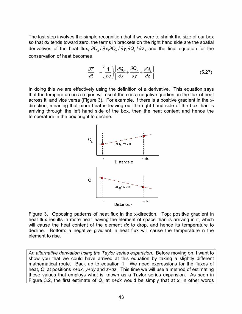
43

The last step involves the simple recognition that if we were to shrink the size of our box so that dx tends toward zero, the terms in brackets on the right hand side are the spatial derivatives of the heat flux,

∂Qx / ∂ x,∂Qy / ∂y,∂Qz / ∂z , and the final equation for the conservation of heat becomes

∂T∂t

= − 1ρc

⎛⎝⎜

⎞⎠⎟

∂Qx

∂x+∂Qy

∂y+∂Qz

∂z⎧⎨⎪

⎩⎪

⎫⎬⎪

⎭⎪ (5.27)

In doing this we are effectively using the definition of a derivative. This equation says that the temperature in a region will rise if there is a negative gradient in the flux of heat across it, and vice versa (Figure 3). For example, if there is a positive gradient in the x-direction, meaning that more heat is leaving out the right hand side of the box than is arriving through the left hand side of the box, then the heat content and hence the temperature in the box ought to decline.

Figure 3. Opposing patterns of heat flux in the x-direction. Top: positive gradient in heat flux results in more heat leaving the element of space than is arriving in it, which will cause the heat content of the element dx to drop, and hence its temperature to decline. Bottom: a negative gradient in heat flux will cause the temperature n the element to rise. An alternative derivation using the Taylor series expansion. Before moving on, I want to show you that we could have arrived at this equation by taking a slightly different mathematical route. Back up to equation 1. We need expressions for the fluxes of heat, Q, at positions x+dx, y+dy and z+dz. This time we will use a method of estimating these values that employs what is known as a Taylor series expansion. As seen in Figure 3.2, the first estimate of Qx at x+dx would be simply that at x, in other words

44

Qx(x+dx) = Qx(x). A second, better estimate would entail projecting the slope of the function Q over the distance dx. This would yield Qx(x+dx) = Qx (x) + (dQx/dx * dx). You can see from the figure that this ought to yield a better estimate. Better yet, you might take into account the curvature of the function. A Taylor series expansion formalizes this process of estimation:

Q(x + dx)=Q(x) + ∂Q∂xdx + 1

2∂2Q∂x 2

dx( )2 + ... 1n!

∂nQ∂xn

dx( )n (5.28)

Note that as we take smaller and smaller elements, as we shrink our control volume, the terms with dx2, dx3 and so on, will become very small very fast. These are called “higher order terms”, and they may be neglected in the limit as dx->0.

Figure 2. Taylor series expansion. Estimation of the value of the function Q at a position x+dx. The first guess would be the value of the function at a nearby point x (lower blue dot). The second estimate acknowledges the rate of change of the function at x, and projects the rate of change over the interval dx (second blue dot). A third estimate would include the curvature of the function at x (third blue dot), and so on. The Taylor series expansion includes all of these terms in the estimate. As the distance dx over which these projects or extrapolations are being made shrinks (i.e., as dx-> 0), the role of the higher order terms declines, and it is sufficient to use simply the local gradient, the first derivative, in the estimation.

Neglecting these higher order terms, when this estimate and the comparable ones for Qy(y+dy) and Qz(z+dz) are inserted into equation 1, it becomes

∂(ρcTdxdydz)∂ t

= Qx(x)dydz − Qx(x)+∂Qx

∂xdx

⎛⎝⎜

⎞⎠⎟

dydz +Qy (y)dxdz − Qy (y)+∂Qy

∂ydy

⎛

⎝⎜

⎞

⎠⎟ dxdz

+Qz(z)dxdy − Qz(z)+∂Qz

∂zdz

⎛⎝⎜

⎞⎠⎟

dxdy

(5.29)

Performing the subtractions yields

∂(ρcTdxdydz)∂t

= −∂Qx

∂xdxdydz −

∂Qy

∂ydydxdz −

∂Qz

∂zdzdxdy (5.30)

45

Dividing by ρcdxdydz, we arrive again at equation 3. The two mathematical routes have converged at the same equation for conservation of heat. From this point on, we will assume that the heat problem is one-dimensional, and vertical, in only the z direction. This will allow us to ignore gradients in heat flux in the horizontal dimensions x and y. As we see below, this situation arises when the gradients in temperature are small in the horizontal relative to those in the vertical. As yet, we have not identified the specific process by which heat is transported in the medium. There are three means of heat transport: conduction, advection, and radiation. Radiation requires that the medium of concern is at least partially transparent (hence translucent) in the proper wavelengths, which rock and soil certainly are not. Advection requires that the medium, or another fluid passing through it, be in motion. For now we are assuming that this is not the case. The principal means by which the near-surface rock is cooled is therefore by conduction. Vibrational energy is traded off between adjacent atoms in such a way as to even out the energy, meaning that it flows from regions of high energy (temperature) to regions of low temperature. The result is a relationship that has become known as Fourier's law, in which the flux of heat in a particular direction, say along the x-axis, is proportional to the local gradient of temperature in that direction, through a constant called the thermal conductivity, k.

Qz = −kz∂T∂z

(5.31)

This heat flux has units of energy per unit area per unit time. The minus sign assures that the heat travels down thermal gradients, from hot toward cold. When we combine this expression for the heat flux with the 1-D equation for conservation of heat, we obtain

∂T∂t

= − 1ρc

⎛⎝⎜

⎞⎠⎟

∂(−k∂T / ∂z)∂z

⎧⎨⎩

⎫⎬⎭

(5.32)

If the thermal conductivity of the material is uniform in the z-direction (k(z) = constant, we may remove k from the partial derivative, and the equation may be simplified to

∂T∂t

=κ ∂ 2T∂z2

(5.33)

Here I have defined κ = k / ρc as the thermal diffusivity. This is the diffusion equation, in which the rate of change of temperature is governed by the local curvature of the temperature profile. Diffusion equations – for anything – arise by combining statement

46

for conservation of some quantity, and a transport rule for that quantity that involves spatial gradients.

The steady geotherm Now we need to give this equation some exercise: we seek solutions for specific situations. We start with the simplest case: the steady geotherm. This is the expected steady temperature profile in the earth’s crust. In steady cases, we assume that any partial derivatives with respect to time are zero. In this case, the left hand side is therefore zero, leaving

d 2Tdz2

= 0 (5.34)

Note that this step has reduced the partial differential equation (PDE) to an ordinary differential equation (ODE); in recognition of this, the partial symbol

�

∂ /∂z has become d/dz. Without any more math we can already extract some in=sight into the solution. This equation says that the curvature is zero. A function that does not curve is a straight line. Our only task now is to assess which of all possible straight lines to choose. In order to solve for T(z), we must integrate this equation twice. Each integration will require appeal to a boundary condition to solve for the constant of integration. Integrating both sides of this equation for the first time results in an equation for the slope of the temperature profile, the gradient

∂T∂z

= c1 (5.35)

where c1 is the constant of integration. Here we appeal to Fourier’s Law to assess the gradient, c1. Rearrangement of equation 7 suggests that the gradient is set by the ratio of the heat flux and the conductivity:

∂T∂z

= −Qk

(5.36)

As it is customary to define the near-surface heat flux as positive upward, despite having defined depth as positive downward. We therefore use Qm= -Q to alter this equation to:

∂T∂z

=Qm

k (5.37)

where Qm signifies the mantle-derived heat flux. The second integration results in

T =Qm

kz +c2 (5.38)

47

One can see that this second constant of integration must have units of temperature. We use again a boundary condition, a place at the edge of the space of concern at which we know something about the system. Here it is the temperature. The most obvious choice is to take the mean annual ground surface temperature, Ts , which we might know from the local climatology. That temperature is being set by completely different physics than the temperatures at depth. It is set by the energy balance at the earth’s surface (which we have already dealt with in prior lectures). Substituting T(0)=

Ts suggests that c2= Ts , resulting in the final equation for the temperature profile:

T =Ts +Qm

kz (5.39)

This is the linear geotherm we expect in the steady state situation we have described. Combinations of thermal conductivity and mantle heat flux result in typical geothermal gradients on the order of 25-30°C/km.

Permafrost Let’s make use of this equation in cold regions. Consider what sets the base of the permafrost. By definition, permafrost is permanently frozen ground, in which the temperature does not rise above 0°C over several years. We can solve the above equation for the depth of the base of the permafrost by solving the equation for z, and setting the temperature to be T = 0°C. The solution is:

zb = −TskQm

= −Ts

dT / dz (5.40)

For example, if the temperature gradient is 25°C/km, and the mean annual temperature is -30°C, the base of the permafrost is 30/25 = 1.2 km. Everything between about 1 or 2 m (the base of the active layer that annually freezes and thaws) and 1200 m depths is frozen stiff, “permanently”. Note that this material does not have to contain water; the temperature simply has to be such that any water that does exist is in the form of ice. In Figure 4 the temperature profiles for several mean annual surface temperatures are shown, along with the resulting relationship between mean annual temperature and the depth to the base of the permafrost.

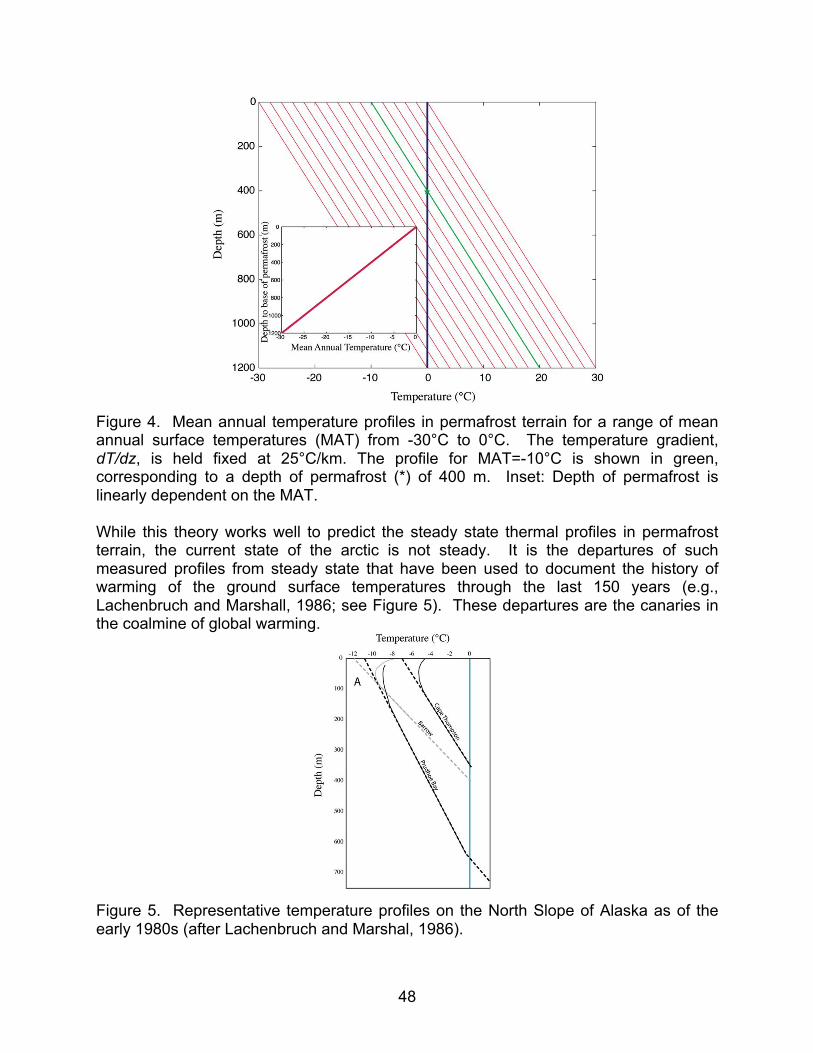
48

Figure 4. Mean annual temperature profiles in permafrost terrain for a range of mean annual surface temperatures (MAT) from -30°C to 0°C. The temperature gradient, dT/dz, is held fixed at 25°C/km. The profile for MAT=-10°C is shown in green, corresponding to a depth of permafrost (*) of 400 m. Inset: Depth of permafrost is linearly dependent on the MAT. While this theory works well to predict the steady state thermal profiles in permafrost terrain, the current state of the arctic is not steady. It is the departures of such measured profiles from steady state that have been used to document the history of warming of the ground surface temperatures through the last 150 years (e.g., Lachenbruch and Marshall, 1986; see Figure 5). These departures are the canaries in the coalmine of global warming.

Figure 5. Representative temperature profiles on the North Slope of Alaska as of the early 1980s (after Lachenbruch and Marshal, 1986).

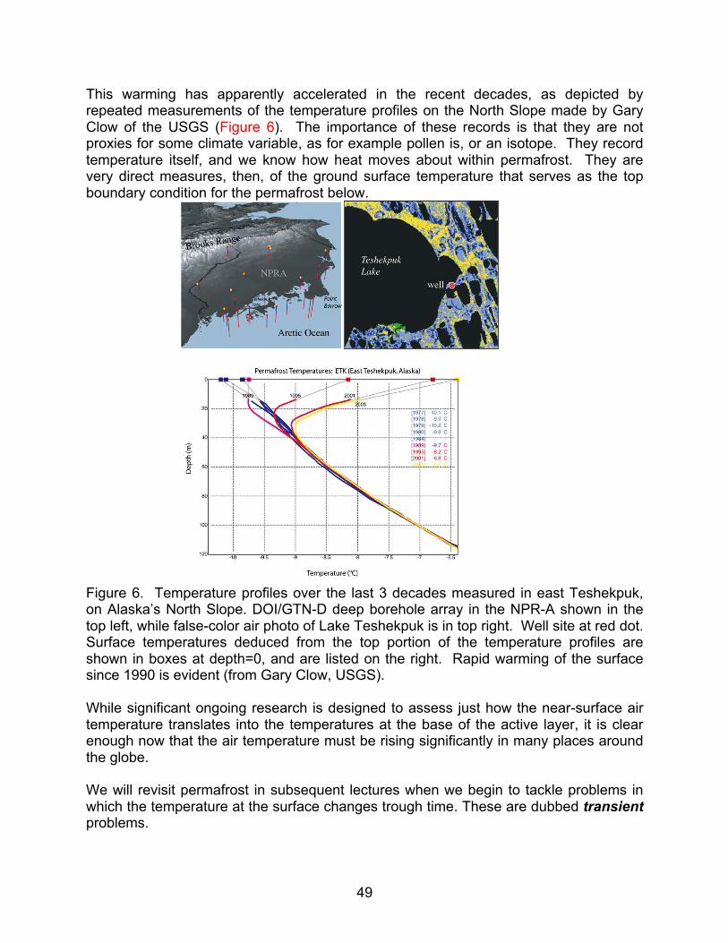
49

This warming has apparently accelerated in the recent decades, as depicted by repeated measurements of the temperature profiles on the North Slope made by Gary Clow of the USGS (Figure 6). The importance of these records is that they are not proxies for some climate variable, as for example pollen is, or an isotope. They record temperature itself, and we know how heat moves about within permafrost. They are very direct measures, then, of the ground surface temperature that serves as the top boundary condition for the permafrost below.

Figure 6. Temperature profiles over the last 3 decades measured in east Teshekpuk, on Alaska’s North Slope. DOI/GTN-D deep borehole array in the NPR-A shown in the top left, while false-color air photo of Lake Teshekpuk is in top right. Well site at red dot. Surface temperatures deduced from the top portion of the temperature profiles are shown in boxes at depth=0, and are listed on the right. Rapid warming of the surface since 1990 is evident (from Gary Clow, USGS). While significant ongoing research is designed to assess just how the near-surface air temperature translates into the temperatures at the base of the active layer, it is clear enough now that the air temperature must be rising significantly in many places around the globe. We will revisit permafrost in subsequent lectures when we begin to tackle problems in which the temperature at the surface changes trough time. These are dubbed transient problems.

50

Summary questions What are the basic steps involved in setting up the heat equation? What assumptions are made along the way? (there are several) What governs the geotherm on the Earth? (what physics and what constants are required, and what assumptions are made?) Can the geotherm be extrapolated to the whole Earth…and why not? Note: Much of this lecture is reprinted from the 1st chapter in The Little Book of Geomorphology, available on the web since 2008.

51

The role of radioactivity in altering the thermal structure of the crust Review of the geotherm Last time we developed the heat equation, and then began to exercise it. Recall that the heat equation involved a statement of conservation of heat, followed by an assumption that the heat flows by conduction in the problems we will be treating here. The statement of conservation left us with a left hand side representing the rate of change of heat content in our control volume. On the right hand side we found terms that represent the gradients of heat flux across opposite sides of the box – in the x, y and z directions -- plus a final term that allowed for the possibility of heat production or consumption in the control volume. And recall that those gradient terms were negative gradients. We talked about why they were negative. The conservation statement had temperature visible on the left but no temperatures on the right. We transformed the right hand side terms to those with temperature – a process called “closing” the equation -- using a relation between the fluxes and temperature. In particular we chose to close the equation using Fourier’s Law in which the heat flux is the product of thermal conductivity and the temperature gradient in the direction of the flux. And again it has a negative sign, which assures us that heat moves from hot to cold. These two steps resulted in the famous diffusion equation relating the rate of change of temperature to the curvature of the temperature field in all three directions, plus a source or sink term.

∂T∂t

=κ ∂2T∂x2 +κ ∂2T

∂y 2 +κ∂2T∂z2 + A

ρc (6.41)

This equation is a 2nd order linear partial differential equation. We first showed that this works as it should, killing strong spikes or bumps in a temperature profile, replacing them with smoother and smoother profiles through time. This meets our expectations both physically and mathematically, and justifies our impression of what diffusion should do: smooth things. We then chose to work the simplest possible problem, generating the geotherm in the top portion of the Earth’s crust. We asked what the temperature profile would look like (in z, depth into the earth) if the temperature at the surface were held steady, and if there were no sources of heat. If the solution is steady, the left hand side may be set to zero. If the problem is 1D, terms in x and y disappear. And if there is no heat source the last term disappears. This left us with one term on the right hand side, the curvature of temperature w.r.t. (with respect to) z, equal to zero. We then integrated this twice, and asserted boundary conditions to solve for the constants of integration associated with each integration. The first boundary condition corresponds to a temperature gradient, which we found by imposing Fourier’s Law. We employed the heat flux from

52

the mantle, Qm, and the conductivity of rock, k. The final boundary condition was the surface temperature, Ts. The resulting equation we call the geotherm:

T =Ts +

Qm

kz (6.42)

Temperature increases linearly with depth into the Earth at a rate governed by the heat flux from the mantle and the local thermal conductivity, pinned to be the long-term average surface temperature at that location.

Figure 1. The geotherm in the absence of radioactive heat sources. This plot was constructed assuming that Qm=50 mW/m2, k = 2W/m-K, and Ts = 15°C. We can exercise this equation in several ways. First calculate the temperature that a miner might experience while attempting to extract ore from one or more famous mining districts – say the Comstock lode in Nevada, or the gold mines of the Rhodesia (Zimbabwe since 1980).

53

Figure 2. Rhodesia was named for this man: Cecil Rhodes. Second, we can calculate the depth of permafrost. See the permafrost chapter in the Little Book. But know that permafrost is perennially frozen ground, which occurs in landscapes where the mean annual temperature is below zero. The ground is therefore frozen to depths where the temperature rises to 0°C. So here you need to rearrange the geotherm equation, and solve for depth rather than temperature, knowing that the temperature at that depth is 0°C. Third, we can estimate how deep into the planet one might expect to go before common minerals melt if this thermal structure were to hold. Quartz, say, is common, and melts at temperatures of about 600°C. If the temperature gradient were 25°C/km, we can rearrange our geotherm equation to yield a depth at which this specific temperature is found. We get 23 or 24 km depth depending on the chosen surface temperature (as we see in the plot). Think about whether this makes sense given what you have been told about the structure of the planet. Bottom line: it does not.

Role of radioactivity in the crust Now we will allow a role for the last term in the diffusion equation, the source term. So far we have neglected this, and arrived at nice simple straight geotherms. We can work two problems, one the role of radioactivity in the earth’s crust, the other the role of solar energy that penetrates into ice covering a lake or the ocean. What are the sources of heat within the crust of our planet? Below the first few meters, within which water can change phase from liquid to solid, the main heat source is radioactive decay of elements in the rock. The radioactive elements we need to be concerned with are those with long half-lives, which will therefore still be decaying at the age of the earth, 4.6 billion years (Ga), and therefore still around as heat sources. These elements are dominated by 238U an 232Th (see tables in Davies), with half-lives of 4.47 and 14.01 Ga, respectively, and by 40K. As they are large incompatible elements, they are incorporated only melts that crystallize

54

late, and hence are found in upper level, crustal rocks. According to Davies’ Table 7.2, heat production by such elements is 1000-fold greater in crustal vs mantle rock. Accounting for the possibility of heat production, our diffusion equation, again in the steady 1D case, becomes

0 =κ d 2T

dz2 + A(z)ρc

(6.43)

In order to integrate this we must assert (or guess) some dependence of the heat source A on z. In Turcotte and Schubert they treat a couple forms. We will employ the exponential dependence, as it gives us practice in use of exponentials that we will see many times over the semester. It is also justified as a functional form in that it is robust against the erosion history at a site. Let us therefore chose the form

dTdz

=A0kz*e

−(z/z* ) + c1 (6.44)

Here the A0 represents the heat production rate per unit mass per unit time in a sample of rock taken from the surface (when z=0, e-0 = 1), and z* is a characteristic depth. In particular, it is the depth to which one must go in the earth before the heat production rate has fallen to e-1 or 1/e or roughly 1/3 of that at the surface. Get used to this; we will very often employ this sort of scaling of exponential functions. Our task now is to integrate the diffusion equation with this specific form for the distribution of heaters. We will have to do this twice, each time employing something we know about the problem to solve for the constants of integration. 1st integration. Recalling that the integral of an exponential is an exponential, we obtain

dTdz

=A0

kz*e

−(z/z* ) + c1 (6.45)

where c1 is a constant of integration. The k is thermal conductivity – I have employed the definition of thermal diffusivity here. We have to solve for this constant before we can proceed to integrate the second time. The units of c1 are a temperature gradient. Where do we know something about the gradient? At great depths, below all these crustal heaters, we can employ the same temperature gradient we employed to arrive at the geotherm. By great depths, I really mean here when z>>z*. At that depth the exponential term vanishes. Formally, we say that the boundary condition we use is when z>>z*, dT/dz = Qm/k. Plugging these into our equation we see that

Qm

k=

A0

kz*

⎛⎝⎜

⎞⎠⎟

0 + c1 = c1 (6.46)

55

so that we may simply replace c1 in equation 4 with Qm/k:

dTdz

=A0

kz*e

−(z/z* ) +Qm

k (6.47)

We’ll return to this in a moment to think about what this looks like and why. But for now, let’s integrate a second time. 2nd integration. We obtain

T = −A0z*

2

ke−(z/z* ) +

Qm

kz + c2 (6.48)

Once again we must solve for the constant of integration, here called c2. This time the dimensions of the constant are temperature, so we seek a position where we know something about the temperature. Again, we can use the fact that at the surface, where z = 0, we impose a steady surface temperature, Ts. Inserting this into our equation, we see that

c2 =Ts +A0z*

2

k (6.49)

and inserting this into equation 7 yields

T =Ts +

Qm

kz +

A0z*2

k1− e−(z/z* )( ) (6.50)

OK. Now we have our solution! Let’s now plot it, think about it, make sure it makes sense in all ways – physically and mathematically… and then exercise it. Let’s first inspect the math. The fist two terms of the solution look like our good old geotherm, a straight line increasing with depth. If A0=0, and there are no heaters, in fact this is the solution. And that better be the case, right? In other words, we have recovered the simpler case. As the parameters collected in front of the last term are all positive, it looks like the temperatures at all depths will be above the geotherm if there are radioactive heaters in the crust. But what does this solution look like graphically? Let’s break out that last term and explore it. Use the math appendix from our book (A&A) to examine what a function y=B(1-e-(x/x*)) looks like. This is a classic example of an asymptotic function. Here it starts at 0 when x = 0, and asymptotically approaches B when x>>x*. And at a specific location x = x*, the value of the function is B/e or roughly B/3 (given that e = 2.7172…).

56

Figure 3. Bending of the straight geotherm (dashed) by the presence of exponentially distributed radioactive elements (red). We can now see the role of the heaters. They increase the temperatures everywhere, increasingly so at depth. But their effect is finite, as it asymptotically reaches a maximum offset at several times the characteristic depth scale – here z* = 8 km. Now consider what is going on physically. There are no heaters below a few z*, so the gradient of temperature, dT/dz, must simply pass the heat from the mantle, Qm. At shallower depths, the gradient must increase to accommodate all additional heat produced beneath that depth. The thermal gradient must therefore increase all the way to the surface. We can see this as well in our equation 6 for the temperature gradient. In fact, at the surface, where z = 0, the temperature gradient is

dTdz

=Qm

k+

A0z*

k (6.51)

The temperature gradient has increased by an amount A0z*/k. Given our formula for heat flux, Fourier’s Law, we can also calculate the heat flux at the surface by multiplying both sides by k:

Qs = Q(z = 0) = − Qm + A0z*( ) (6.52) where the minus sign reflects the fact that the heat is flowing in the negative z direction, or upward, out of the earth. This equation allows us to calculate what is called the reduced heat flux as an estimate for the mantle heat flux. Qm = Qs − A0z* (6.53) But how does one put this into operation? One must measure the surface heat flux at a location, using the local near-surface gradient say documented in a mine or a borehole

57

and a measure of the conductivity, k, measure the heat production rate in a surface sample, A0, and have some independent measure of z*. But this last item is hard to come by! Instead, we sample many locations in the region we suspect ought to have the same mantle heat flow, and hope to have a scatter of measured Qs and A0. When we plot them using equation 12, with Qs on the y-axis and A0 on the x-axis. The y-intercept is then the mantle heat flow, and the slope is z*. Pretty cool, eh? When this is done for the Sierras, as replicated in T&S, one obtains a depth scale z* of a few kilometers.

Thermal profiles in lake and sea ice: An example of absorption in translucent materials of uniform properties One may also address a problem of similar complexity involving a different source of heat source: the absorption of radiation in a partially transparent substance, here ice. Again, following our theme of simplicity, we assert that the system has achieved a steady thickness of ice, and that the profile of temperature within the ice is not changing. We are left with the same two terms in our diffusion equation, but now need both a description of the absorption of solar radiation with depth, and proper boundary conditions. Here we ask what governs the profile of temperature in the ice lid on a permanently frozen lake. Such lakes are found in the Dry Valleys of Antarctica, where the lake ice thickness varies from one to the other, commonly a few meters, but is relatively steady in each (McKay et al., 1985). This problem involves conduction of heat through the ice, production of heat within the ice by absorbed sunlight, heat released at the base of the ice by the change of phase of water into ice, and sublimation loss from the top of the ice. We start with the 1D heat conservation equation

∂T∂t

= − 1ρc

∂Q∂z

+ A(z)ρc

(6.1)

where T is temperature, t time, z depth, Q the heat flux [W/m2], A a heat source [W/m3], and ρ and c are the material density and heat capacity, respectively.

58

Figure 4. Schematic for lake ice calculation. At steady state, the rate of sublimation must equal the rate of freeze-on at the base of the ice. Attenuation of radiation with depth is characterized by the attenuation length h. Our development from this point onward mirrors that in McKay et al. (1985). They suggest that the lake ice is maintained at an annually averaged steady state thickness, H. In this steady case the ice lost off the top of the ice cover by ablation (or sublimation) must equal the new ice that is frozen onto the base of the ice. The rate of freeze-on is governed by the rate at which heat can be removed from the basal boundary by conduction through the ice lid, and hence by the gradient in T with depth, z. Hence we must assess the expected T(z) profile. The rate of release of latent heat by the phase change is

ρL ∂z

∂t (6.1)

where L is the latent heat energy released per unit mass of water converted to ice. Given that at steady state the rate of freeze-on must equal the ablation rate, ν (Figure 1), the heat flux boundary condition at the base of the ice must be

Q = −k ∂T∂z

= ρL ∂z∂t

= ρLν (6.2)

Here the first statement is simply Fourier’s Law. We can immediately see that the temperature gradient at the base of the ice must increase as the ablation rate increases. An additional complexity is that sunlight can penetrate into the translucent ice, and is absorbed as it does so. That absorbed radiation serves as a heat source that is depth-dependent. According to the Beer-Lambert law (eq. 6), the source term in the conservation of heat equation will be

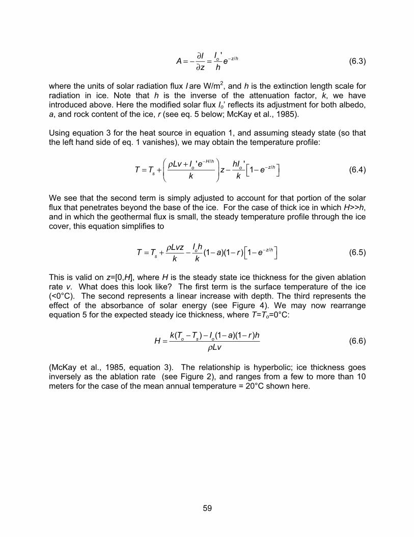
59

A = − ∂I

∂z=

Io 'h

e−z/h (6.3)

where the units of solar radiation flux I are W/m2, and h is the extinction length scale for radiation in ice. Note that h is the inverse of the attenuation factor, k, we have introduced above. Here the modified solar flux Io’ reflects its adjustment for both albedo, a, and rock content of the ice, r (see eq. 5 below; McKay et al., 1985). Using equation 3 for the heat source in equation 1, and assuming steady state (so that the left hand side of eq. 1 vanishes), we may obtain the temperature profile:

T =Ts +

ρLv + Io 'e−H /h

k⎛

⎝⎜⎞

⎠⎟z −

hIo 'k

1− e−z/h⎡⎣ ⎤⎦ (6.4)

We see that the second term is simply adjusted to account for that portion of the solar flux that penetrates beyond the base of the ice. For the case of thick ice in which H>>h, and in which the geothermal flux is small, the steady temperature profile through the ice cover, this equation simplifies to

T =Ts +ρLvzk

−Iohk(1− a)(1− r ) 1− e−z/h⎡⎣ ⎤⎦ (6.5)

This is valid on z=[0,H], where H is the steady state ice thickness for the given ablation rate v. What does this look like? The first term is the surface temperature of the ice (<0°C). The second represents a linear increase with depth. The third represents the effect of the absorbance of solar energy (see Figure 4). We may now rearrange equation 5 for the expected steady ice thickness, where T=To=0°C:

H =k(To −Ts ) − Io(1− a)(1− r )h

ρLv (6.6)

(McKay et al., 1985, equation 3). The relationship is hyperbolic; ice thickness goes inversely as the ablation rate (see Figure 2), and ranges from a few to more than 10 meters for the case of the mean annual temperature = 20°C shown here.

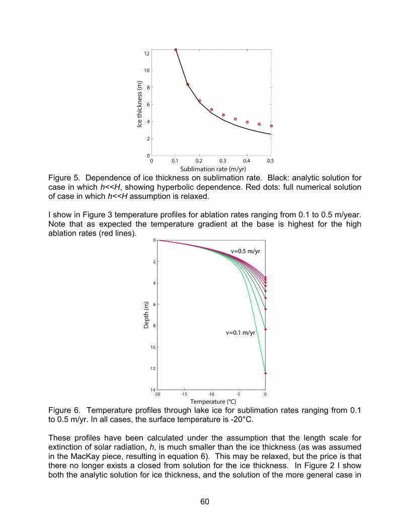
60

Figure 5. Dependence of ice thickness on sublimation rate. Black: analytic solution for case in which h<<H, showing hyperbolic dependence. Red dots: full numerical solution of case in which h<<H assumption is relaxed. I show in Figure 3 temperature profiles for ablation rates ranging from 0.1 to 0.5 m/year. Note that as expected the temperature gradient at the base is highest for the high ablation rates (red lines).

Figure 6. Temperature profiles through lake ice for sublimation rates ranging from 0.1 to 0.5 m/yr. In all cases, the surface temperature is -20°C. These profiles have been calculated under the assumption that the length scale for extinction of solar radiation, h, is much smaller than the ice thickness (as was assumed in the MacKay piece, resulting in equation 6). This may be relaxed, but the price is that there no longer exists a closed from solution for the ice thickness. In Figure 2 I show both the analytic solution for ice thickness, and the solution of the more general case in

61

which the assumption of H>>h is relaxed. We see that the analytic solution is sufficiently accurate for small sublimation rates (and hence large ice thickness), but is no longer accurate for large sublimation rates. In these cases one must find the appropriate ice thickness by calculating a set of T(z) profiles using equation 4 for a range of chosen H’s, and choosing that in which the temperature at z=H, at the base of the ice, is the required To=0°C. (This is done in the Matlab code lake_ice_temperatures_iterate.m). Interestingly, since the ice thickness is tied to the sublimation rate, we can assess for any case the residence time of the ice. It accumulates at the base and is lost at the top. The full residence time is therefore H/v. For the cases shown here, the residence time increases from 6 years to 120 years as the ablation rate declines from 0.5 to 0.1 m/year. The thicker ice therefore has a longer record of the chemistry and biology of the lake embedded in (frozen into) the ice lid. We can see from this example of an ice lid on a lake the role for both the latent heat associated with the phase change of water, and the role for deposition of solar heat within the ice associated with its translucence.

62

Transient problems I: Thermal profiles driven by oscillating surface temperatures, or The snake writhing in an exponential funnel Introduction to transient problems In the first few lectures we have explored a range of steady problems, by which I mean that the temperature at the surface of the object of concern –here the planet – has been kept steady for a long time so that at no point in the object is the temperature changing. We are now going to relax that assumption, and explore a variety of cases that we dub transient problems. In these the temperature at the surface is no longer held steady, and hence the temperatures at depth can never be truly steady either. Or at least in some region sufficiently close to the surface such variations will be “felt”. First let us imagine some scenarios in which the surface temperature is not constant. How might it vary? Can you think of a few cases – and sketch them out as histories of temperature at the surface, Ts(t)? I think you will agree that there are many possible histories. It is our task first to catalog a few of these, and then to describe them mathematically. Graph your own choice of a proposed temperature history at the surface here… in class exercise…and then propose how to describe that history mathematically. We will treat two specific cases that together encompass a wide range of geologic scenarios. These are cases in which the surface temperature oscillates sinusoidally (or is said to be periodic), or in which the surface temperature either drops or rises abruptly (the cases of instantaneous heating or cooling). Both of these transient problems are tractable without appeal to a numerical model. In other words, we will derive an analytic solution, one that can be written down with chalk or a pencil. The two classes of problems include the following: for periodic forcing, both the daily and the annual oscillation in surface temperature can be well captured by sinusoidal functions. We can ask more specifically such questions as: how deeply does it freeze? How deeply does it thaw on an annual basis in permafrost regions – a depth we call the active layer thickness? For instantaneous change at the surface, cases include cooling or even freezing of a lake, warming of permafrost due to global change, cooling of an intrusive dike, heating of a grilled cheese sandwich, cooking of a turkey. In fact, all cooking effectively entails instantaneous increase of the surface temperature of the object we wish to cook – be it an egg, a turkey, or a loaf of bread.

63

Periodic variations in surface temperature Rather than develop the solution for the diffusion equation for this particular case, as is done completely in Turcotte and Schubert, we will use the following strategy: state what the history of temperature is at the surface, then propose a plausible solution, and then see if it works by plugging it into the diffusion equation. Here again is the diffusion equation that governs how heat is transported by conduction within the material, in the absence of heat sources or sinks:

∂T∂t

=κ ∂2T∂z2 (7.1)

We now propose that the temperature history at the surface is sinusoidal:

T(0,t) =T + ΔT sin 2πt

P⎡

⎣⎢

⎤

⎦⎥ (7.2)

where T is the mean temperature at the surface, P is the period of the oscillation and ΔT is the amplitude at the surface (z=0). The maximum temperature is T + ΔT and the minimum temperature is T -ΔT. This serves as the boundary condition for the problem. We expect the temperature to be sinusoidal at depth as well, but with a different amplitude, and perhaps to be lagged in time relative to the temperature history at the surface. We therefore posit a solution that captures this expectation:

T(z,t) =T + ΔTe−z/z* sin 2πt

P− z

z *⎡

⎣⎢

⎤

⎦⎥ (7.3)

where z* is a so-far-undetermined depth scale that scales the decline in amplitude and the lag with depth. Here the amplitude, represented by the collection of symbols in front of the sine, is governed by an exponential decline in amplitude with depth. And the phase shift, also called the lag, represented by the symbols after the 2πt/P, is proposed to increase linearly with depth. Our next task is to determine whether this is indeed a solution to the diffusion equation, and under what conditions it is a solution. To do this we need to differentiate this equation 3 with respect to t to obtain the left hand side of the diffusion equation (1), and then differentiate the solution with respect to z two times (in other words, take its second derivative), and then plug that times the diffusivity into the right hand side of equation 1. All of this is pretty good practice to dredge back into your calculus! I recommend breaking up into two teams, the time derivative team and the spatial derivate team (who will have twice the work to do!). Differentiation with respect to t:

64

∂T∂t

= 2πΔTP

e−z/z* cos2πtP

− zz *

⎡

⎣⎢

⎤

⎦⎥ (7.4)

First differentiation with respect to z:

∂T∂z

= − 1z *

⎡

⎣⎢

⎤

⎦⎥ΔTe

−z/z*⎧⎨⎪

⎩⎪

⎫⎬⎪

⎭⎪sin

2πtP

− zz *

⎡

⎣⎢

⎤

⎦⎥ + ΔTe−z/z* − 1

z *⎡

⎣⎢

⎤

⎦⎥cos

2πtP

− zz *

⎡

⎣⎢

⎤

⎦⎥

⎧⎨⎪

⎩⎪

⎫⎬⎪

⎭⎪

= − ΔTz *e−z/z*

⎧⎨⎩

⎫⎬⎭sin

2πtP

− zz *

⎡

⎣⎢

⎤

⎦⎥ + cos

2πtP

− zz *

⎡

⎣⎢

⎤

⎦⎥

⎛

⎝⎜⎞

⎠⎟

(7.5)

Second differentiation with respect to z: ∂2T∂z2

= ΔTz*2

⎡

⎣⎢⎢

⎤

⎦⎥⎥e−z/z* sin

2πtP

− zz *

⎡

⎣⎢

⎤

⎦⎥ + cos

2πtP

− zz *

⎡

⎣⎢

⎤

⎦⎥ + cos

2πtP

− zz *

⎡

⎣⎢

⎤

⎦⎥ − sin

2πtP

− zz *

⎡

⎣⎢

⎤

⎦⎥

⎡

⎣⎢

⎤

⎦⎥

= 2ΔTz*2

⎡

⎣⎢⎢

⎤

⎦⎥⎥e−z/z* cos

2πtP

− zz *

⎡

⎣⎢

⎤

⎦⎥

(7.6)

Setting the time derivative (4) equal to the product of the diffusivity with the second spatial derivative (6) yields, after some algebra, this simple equation:

z* =

κPπ

(7.7)

This means that the right and left sides of the diffusion equation are equivalent as long as the condition represented by equation 7 is honored. This z*, the depth that scales both the amplitude and the lag of the thermal signal, must have a specific form. Returning to equation 3, the proposed solution that we now know is indeed a solution, we see that the amplitude declines exponentially with depth, with a characteristic length scale that goes as the square root of the period. This should sound a little familiar by now. We have found another situation in which length scales go as square roots of time scales. I refer the interested reader to Geoff Davies’ discussion of the square root relationship between time and length scales. We will see this again and again in diffusion or conduction problems. We can also see from equation 3 that the lag of the thermal signal ought to linearly increase with depth. It is instructive to see the solution plotted in a couple different ways. We can plot the temperature profiles with T on the horizontal axis and z vertical (as it is in nature), and plot several profiles corresponding to several different times. Or we can plot several temperature histories, one for each of several depths, on top of one another, in order to visualize the lag with depth. These are shown in Figure 1 A and B, respectively. Or we can make a movie of it. See the code provided to generate these plots and production of the movie.

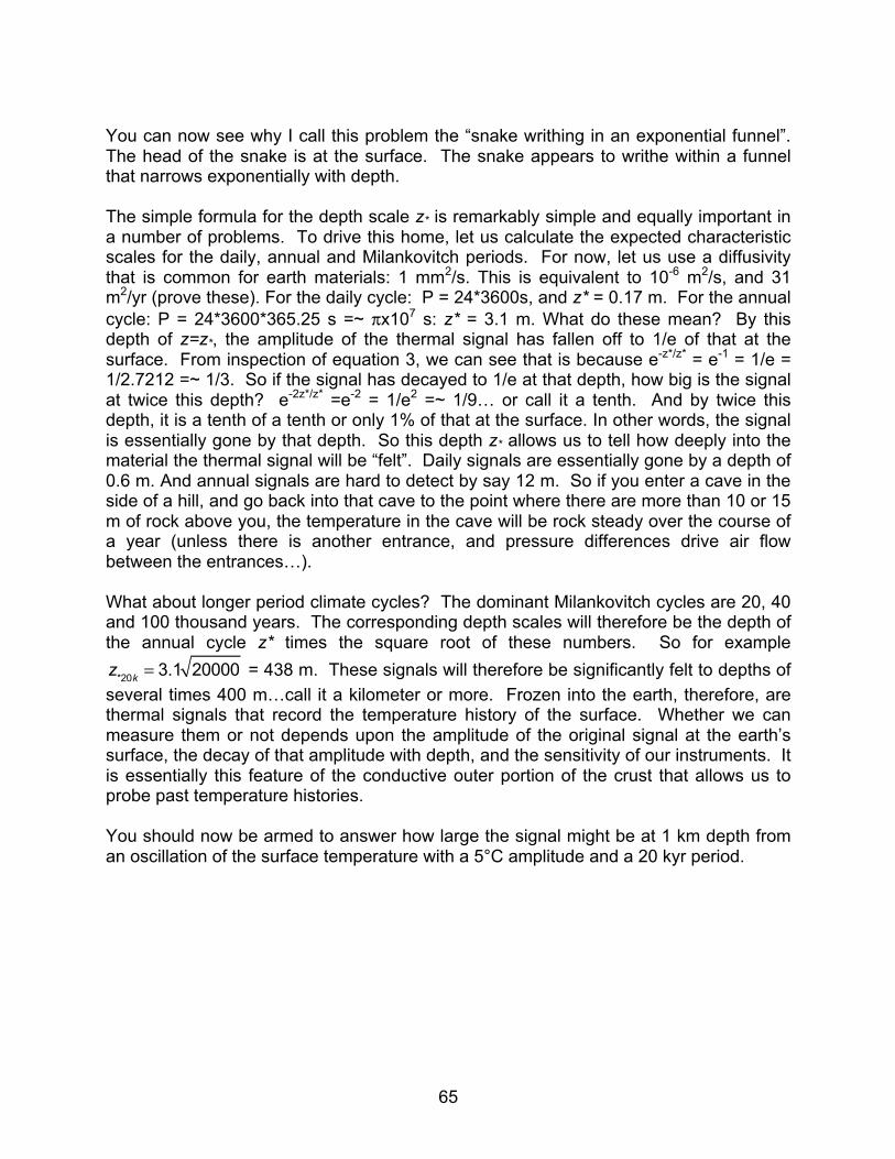
65

You can now see why I call this problem the “snake writhing in an exponential funnel”. The head of the snake is at the surface. The snake appears to writhe within a funnel that narrows exponentially with depth. The simple formula for the depth scale z* is remarkably simple and equally important in a number of problems. To drive this home, let us calculate the expected characteristic scales for the daily, annual and Milankovitch periods. For now, let us use a diffusivity that is common for earth materials: 1 mm2/s. This is equivalent to 10-6 m2/s, and 31 m2/yr (prove these). For the daily cycle: P = 24*3600s, and z* = 0.17 m. For the annual cycle: P = 24*3600*365.25 s =~ πx107 s: z* = 3.1 m. What do these mean? By this depth of z=z*, the amplitude of the thermal signal has fallen off to 1/e of that at the surface. From inspection of equation 3, we can see that is because e-z*/z* = e-1 = 1/e = 1/2.7212 =~ 1/3. So if the signal has decayed to 1/e at that depth, how big is the signal at twice this depth? e-2z*/z* =e-2 = 1/e2 =~ 1/9… or call it a tenth. And by twice this depth, it is a tenth of a tenth or only 1% of that at the surface. In other words, the signal is essentially gone by that depth. So this depth z* allows us to tell how deeply into the material the thermal signal will be “felt”. Daily signals are essentially gone by a depth of 0.6 m. And annual signals are hard to detect by say 12 m. So if you enter a cave in the side of a hill, and go back into that cave to the point where there are more than 10 or 15 m of rock above you, the temperature in the cave will be rock steady over the course of a year (unless there is another entrance, and pressure differences drive air flow between the entrances…). What about longer period climate cycles? The dominant Milankovitch cycles are 20, 40 and 100 thousand years. The corresponding depth scales will therefore be the depth of the annual cycle z* times the square root of these numbers. So for example

z*20k = 3.1 20000 = 438 m. These signals will therefore be significantly felt to depths of several times 400 m…call it a kilometer or more. Frozen into the earth, therefore, are thermal signals that record the temperature history of the surface. Whether we can measure them or not depends upon the amplitude of the original signal at the earth’s surface, the decay of that amplitude with depth, and the sensitivity of our instruments. It is essentially this feature of the conductive outer portion of the crust that allows us to probe past temperature histories. You should now be armed to answer how large the signal might be at 1 km depth from an oscillation of the surface temperature with a 5°C amplitude and a 20 kyr period.

66

Figure 1. A) Temperature profiles in a permafrost setting (mean annual temperature=-10°C < 0°C) recorded at each month of an annual cycle. Temperatures are confined to an exponential envelope. The depth to the base of the active layer atop the permafrost, za (blue dashed line), may be calculated by equating the formula for the maximum T envelope with 0°C. B) Time series of temperatures are the surface (bold) and at depths (denoted, in meters) up to 10 m, showing decline in amplitude and lag with depth. (after A&A Figure 9.5) Returning to the plot of temperature histories at several depths (Figure 1B), note the lag of the thermal signals with depth. Here let’s ask how big this lag is. To be more specific, let’s ask at what depth the lag would be half a period. In other words, if the temperature is at its maximum at the surface, at what depth is the temperature reaching the minimum of its cycle? The argument of the sin() is in radians. How many radians is half a period? There are 2π radians in a full cycle, so only 1π radians in half a cycle. So we can easily figure out this depth by setting the lag, z/z*, to π. In other words, z/z*=π. This means that z=πz*, or about 3 z*. For the daily cycle, for which z*=0.17 m, that is about 0.5 m. And for the annual cycle it is about 10 m. Of course we now know that by that

67

depth the amplitude is pretty small. Formally, the amplitude at this magic depth at which the temperature is exactly out of phase with the surface is e-π, or 0.043, or about 4% of that at the surface. Now try to simulate this with a slow dance. Stand up. Put one arm in the air straight up and make a fist. Make the fist wave back and forth by say a meter steadily. Let’s say your hips are at this magic depth, so must sway in exactly the opposite direction as your fist. To properly simulate the thermal situation, your hips should move only 4% of that by which your fist is waving, or just a few centimeters.

Relevance to the permafrost active layer Let’s apply this to the permafrost setting introduced when we were talking about the steady geotherm. We already have seen that the depth to the base of the permafrost may be calculated easily using the steady geotherm. These depths are usually many tens to many hundreds of meters… well below where these annual signals play a role. But up at the top, the temperature indeed swings significantly over the course of a year, from tens of °C below zero to well above it. This freezes and thaws the topmost layer of the ground. The layer that indeed thaws annually is called the active layer because it can participate in the ecological and hydrological cycle. Here we can ask what governs the depth to the base of the active layer (or the top of what we call the permafrost table). In Figure 3 we see the problem schematically. The depth of the active layer is where the outer right edge of the exponential envelope, which represents the maximum temperature that will be achieved at any depth, equals 0°C. We simply need an expression for that right edge. Noting that we don’t give a hoot about when it achieves this maximum, we can simply set the sin() to 1, and the T on the left hand side to 0. This leaves us with

− TΔT

= e−za /z* (7.8)

where z* is the annual depth scale of order 3 m. We can solve with for the depth za, the base of the active layer, by taking the natural logarithm of both sides and multiplying by –z* we find that

za = −z* ln − T

ΔT⎡

⎣⎢

⎤

⎦⎥ (7.9)

If we choose typical values for the mean and amplitude of the annual temperatures, we find that the active layer is commonly on the order of 1 m thick. examples: thermal data from Laramie range experiment, Wyoming example time series from Fahey site on Niwot Ridge (see animation)

68

Summary questions Describe quantitatively the pieces of the solution for the case of periodic surface

temperatures: mean, amplitude of the oscillation, phase shift (or lag) How does the characteristic depth scale depend upon the period? What is a good diffusivity κ to use? (1 mm2/s) This is worth memorizing!

69

Instantaneous cooling and heating: From the grilled cheese sandwich to the age of the Earth We have just seen an example of one type of transient thermal problem, that in which the surface temperature oscillates. We now visit another example in which the surface temperature is abruptly changed. It could be raised or dropped, after which it remains at that new temperature. If the temperature abruptly drops, we call it an instantaneous cooling problem. If it is instantaneously raised, we call it an instantaneous heating problem. Examples of relevant problems abound in the earth sciences, and indeed in life in general. Let us start by listing a few. A lava flow could flow out across a surface, instantaneously heating it. We might ask how deeply into the surface that heat wave penetrates. Contact metamorphism is all about the country rock being instantaneously heated by coming into contact with a much hotter magma. A forest fire can blaze across a landscape, bringing rock at the surface into contact with air that is now not 20°C but 500°C. For that matter, essentially all cooking entails instantaneously heating some object or substance. In many of these situations we ask how long it might take to reach a new temperature that is some fraction of the newly imposed temperature. In the cooking example, that specific temperature is the one we mean when we call the food “done” and ready to eat. We will visit two example instantaneous cooling problems in the earth sciences. Lord Kelvin suggested one could estimate the age of the earth by working the instantaneous cooling problem in which a molten sphere (the Earth) is instantaneously exposed to a new temperature at the surface of about 0°C. We will also see that the growth of the thickness of the lithosphere away from a spreading ridge can be thought of as an instantaneous cooling problem in which hot mantle is instantaneously exposed to ocean bottom temperatures at the spreading ridge.

Instantaneous cooling problem We will first develop the general problem for cooling. Consider a half space – a volume with one surface and extending infinitely in all other directions away from that surface – in which conduction is the only means by which heat is transported. The reigning equation is therefore our good friend the diffusion equation in one dimension, that normal to the surface:

∂T∂t

=κ ∂2T∂z2 (8.1)

Can you tell me what other assumptions go into this equation? No sources or sinks of heat, and uniform thermal properties.

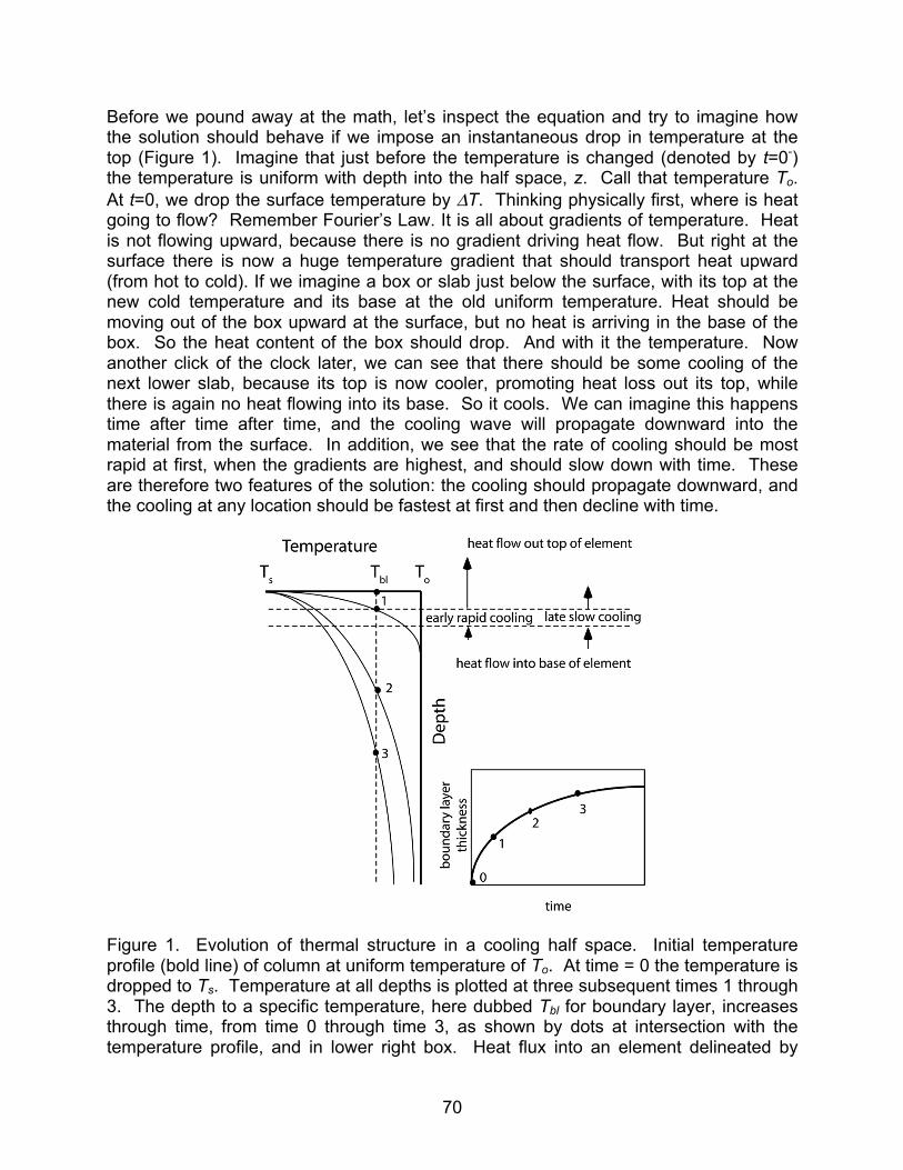
70

Before we pound away at the math, let’s inspect the equation and try to imagine how the solution should behave if we impose an instantaneous drop in temperature at the top (Figure 1). Imagine that just before the temperature is changed (denoted by t=0-) the temperature is uniform with depth into the half space, z. Call that temperature To. At t=0, we drop the surface temperature by ΔT. Thinking physically first, where is heat going to flow? Remember Fourier’s Law. It is all about gradients of temperature. Heat is not flowing upward, because there is no gradient driving heat flow. But right at the surface there is now a huge temperature gradient that should transport heat upward (from hot to cold). If we imagine a box or slab just below the surface, with its top at the new cold temperature and its base at the old uniform temperature. Heat should be moving out of the box upward at the surface, but no heat is arriving in the base of the box. So the heat content of the box should drop. And with it the temperature. Now another click of the clock later, we can see that there should be some cooling of the next lower slab, because its top is now cooler, promoting heat loss out its top, while there is again no heat flowing into its base. So it cools. We can imagine this happens time after time after time, and the cooling wave will propagate downward into the material from the surface. In addition, we see that the rate of cooling should be most rapid at first, when the gradients are highest, and should slow down with time. These are therefore two features of the solution: the cooling should propagate downward, and the cooling at any location should be fastest at first and then decline with time.

Figure 1. Evolution of thermal structure in a cooling half space. Initial temperature profile (bold line) of column at uniform temperature of To. At time = 0 the temperature is dropped to Ts. Temperature at all depths is plotted at three subsequent times 1 through 3. The depth to a specific temperature, here dubbed Tbl for boundary layer, increases through time, from time 0 through time 3, as shown by dots at intersection with the temperature profile, and in lower right box. Heat flux into an element delineated by

71

dashed lines shows large mismatch between heat flowing out top and into base at early times, evolves to much lower mismatch at later times. The large mismatch in temperature causes rapid cooling in early times, decaying to slower cooling rates at later times. (after A&A Figure 3.4) Thinking mathematically instead of physically, recall that the governing equation tells us that rates of change go as the curvature of the temperature profile (equation 1). There is no curvature at depth at first, as the temperatures are uniform. But at the top, immediately after we have turned down the temperature, the curvature is huge (Figure 1). Temperatures therefore ought to change rapidly at first. Armed with this insight into the problem, and some expectations about the behavior of the solution, let us proceed to solve the equation. Again, the full development is well aid out in Turcotte and Schubert. In general, these partial differential equations are hard to solve. In this style of problem we use a trick to convert the PDE to an ordinary differential equation (ODE). We define two dimensionless variables to replace our time and space (z) variables. The first is really just a normalization of the temperature scale so that it just goes between 0 and 1. For this cooling problem, we define a dimensionless temperature to be

θ =

T −Ts

To −Ts

(8.2)

where To is the initial uniform temperature, Ts is the new (colder) surface temperature, and T is temperatures at any other position and time. Make sure that you see that this will indeed be confined to the interval [0 1]. The other variable is more tricky. It combines depth and time by

η = z

2 κ t (8.3)

where t is time since the temperature was turned down at the surface. This is indeed dimensionless. Recall that we have seen repeatedly that length scales go as square roots of kappa times timescales in diffusion problems. This is called the similarity variable for reasons we will discover soon. When we plug these new variables into the diffusion equation (1), the equation is converted to the following ODE:

−η dθ

dη= 1

2d 2θdη2 (8.4)

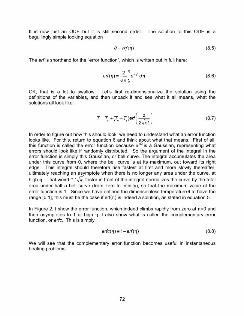
72

It is now just an ODE but it is still second order. The solution to this ODE is a beguilingly simple looking equation θ = erf (η) (8.5) The erf is shorthand for the “error function”, which is written out in full here:

erf (η) ≡ 2

πe−η2

dη0

η

∫ (8.6)

OK, that is a lot to swallow. Let’s first re-dimensionalize the solution using the definitions of the variables, and then unpack it and see what it all means, what the solutions all look like.

T =Ts + (To −Ts )erf

z

2 κ t

⎛⎝⎜

⎞⎠⎟

(8.7)

In order to figure out how this should look, we need to understand what an error function looks like. For this, return to equation 6 and think about what that means. First of all, this function is called the error function because e-x2 is a Gaussian, representing what errors should look like if randomly distributed. So the argument of the integral in the error function is simply this Gaussian, or bell curve. The integral accumulates the area under this curve from 0, where the bell curve is at its maximum, out toward its right edge. This integral should therefore rise fastest at first and more slowly thereafter, ultimately reaching an asymptote when there is no longer any area under the curve, at high η. That weird 2 / π factor in front of the integral normalizes the curve by the total area under half a bell curve (from zero to infinity), so that the maximum value of the error function is 1. Since we have defined the dimensionless temperature θ to have the range [0 1], this must be the case if erf(η) is indeed a solution, as stated in equation 5. In Figure 2, I show the error function, which indeed climbs rapidly from zero at η=0 and then asymptotes to 1 at high η. I also show what is called the complementary error function, or erfc. This is simply erfc(η) ≡ 1− erf (η) (8.8) We will see that the complementary error function becomes useful in instantaneous heating problems.

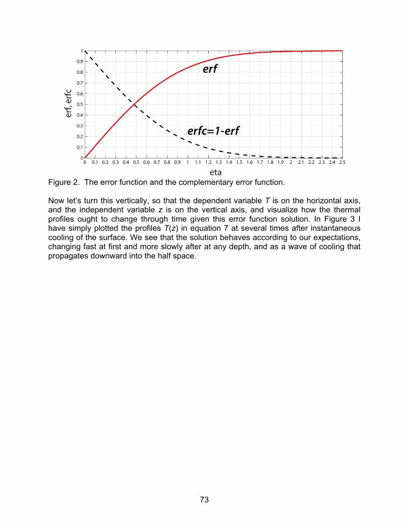
73

Figure 2. The error function and the complementary error function. Now let’s turn this vertically, so that the dependent variable T is on the horizontal axis, and the independent variable z is on the vertical axis, and visualize how the thermal profiles ought to change through time given this error function solution. In Figure 3 I have simply plotted the profiles T(z) in equation 7 at several times after instantaneous cooling of the surface. We see that the solution behaves according to our expectations, changing fast at first and more slowly after at any depth, and as a wave of cooling that propagates downward into the half space.

74

Figure 3. Instantaneous cooling problem. Temperature profiles at several evenly spaced times after cooling begins. Here, these are shown at 10-year intervals up to 100 years after the cooling begins. Initial profile is dashed. One can see that the solution simply looks like the error function plot shown in Figure 2 turned on its side. Importantly, every one of the profiles looks like this. They differ only in being “stretched” a little more with time. This is in fact why we call the variable η a similarity variable. Every profile at any time looks “similar” to any other, differing only in the degree of stretching.

Lord Kelvin and the Age of the Earth We will now exercise this solution. In the late 19th century there raged a debate about the age of the earth. We had no isotopic or radioactive method to employ to date rocks. We had to reply upon inferences derived form rates of sedimentation and thicknesses of sedimentary sections, for example. The community wished to go beyond Hutton’s famous cop-out “…there is no hint of a beginning, no prospect of an end…” statement early in the century. Enter Lord Kelvin. He said hey, this is nothing but an

75

instantaneous cooling problem. It is physics and we know this. Here is how he proposed to view the planet. At initial formation it was molten, so uniform with a temperature something like the melting point of rock. Thereafter the surface temperature has been held at something like what it is now, call it 0°C. And it has been cooling since in the face of this newly imposed boundary condition. But what can we measure that will be a proxy of time? On Figure 4, see what he proposed: while we cannot measure the entire profile, we can measure the topmost section of the profile. And in particular we can measure the gradient of temperature, dT/dz, say in deep mines. He said look, this is an instantaneous cooling problem, and all we need is an equation for the history of the dT/dz measured close to the earth’s surface.

Figure 4. Diagram of the temperature structure of a cooling body through time, and how the temperature gradient close to the surface should evolve. It is this gradient that Lord Kelvin proposed as the proxy for the age of the planet. In equation 7 we have the solution for T(t). All we need to do is differentiate this with respect to z, and evaluate it at z=0. Taking the derivative yields

dTdz

= (To −Ts )πκ t

e− z2 κ t

⎛⎝⎜

⎞⎠⎟2

(8.9)

76

and evaluating this where z=0 leaves us with the simpler equation that is only a function of time:

dTdz z=0

=(To −Ts )

πκ t (8.10)

This can be algebraically manipulated to arrive at a solution for time if we know both the gradient at the surface:

t = 1

πκ(To −Ts )

dT / dzz=0

⎡

⎣⎢

⎤

⎦⎥

2

(8.11)

All that remains is evaluating this using some appropriate numbers. Lord Kelvin used a variety of choices for these parameters over years of publication about the problem, but representative numbers are these: To=1600°C, Ts=0°C, dT/dz at the surface = 25°C/km = 0.025 °C/m, κ=31m2/yr. Lord Kelvin’s result: the age of the earth is 4x108 years of 40 million years. Pretty cool, right? And way wrong. At least now we know it is way wrong. At the time the debate raged, the geologists wanting/needing a much older earth. Much has been written about why Lord Kelvin was wrong. See discussions in Geoff Davies’s chapter 2; see also Carslaw and Jaeger, and England et al. paper on this debate. But the essence is that his analysis did not account for the production of heat by radioactive elements in the earth, and more importantly the major means by which heat is transported in the mantle of the earth is by convection.

Boundary layer defined Ok, let’s ask a different question. You have just poured hot coffee into your coffee mug, one of those with big thick ceramic walls. The mug is at room temperature, call it 20°C. The coffee doesn’t cool off immediately, but instead continues to bathe the inner wall of the mug with fluid at 100°C. It is an instantaneous heating problem. We might ask how far into the mug wall can the change in temperature be “felt”, or how deeply its temperature has been changed significantly. It varies from one problem to another what we mean by “felt” or “significantly”. To be specific, let’s say that in this case to be “felt” means its temperature has been raised by 10°C. This layer in which the material has responded to some fixed degree to a newly imposed condition at a surface is called a boundary layer, so-called because it is near a wall or boundary. We expect that this wave of heat, or here a thermal boundary layer, will move through time, penetrating more and more deeply into the mug wall. And we’d like to know what the history of thickening of the boundary layer should look like. How do we solve for this thickness of a boundary layer whose temperature has been changed “significantly”? See again Figure 1. First, note that this specific temperature corresponds to a specific non-dimensional temperature θbl where the subscript bl signifies boundary layer. And in the solution of our transient problem there arises a

77

relationship between θ and η through the error function. Once we know a specific θ, we can solve for a specific η. Returning to the definition of our similarity variable η, we can now solve for the relationship between z and t because η is now a constant value:

ηbl =

z2 κ t

(8.12)

This is easily solved for the history of the boundary layer thickness zbl(t): zbl = 2ηbl κ t (8.13) This is a profound result. Not just in this case, but in all cases, boundary layers in diffusion problems increase in thickness at the square root of time, the specific rate being governed by the specific temperature of concern that set θbl and hence ηbl in equation 13.

Instantaneous heating problems As you might imagine, the heating problem is perfectly analogous to cooling problems. We expect it to have the same sort of shape and the same time behavior, but somehow it has to be flipped or backwards. Let’s carry out the same analysis and see what happens. The first task is to define a different non-dimensional temperature. Remember this must have a range of [0 1]. Inspection of the problem set up suggests that we define

θ =

T −To

Ts −To

(8.14)

Assure yourself that this is indeed positive everywhere, and is limited by [0 1]. The boundary conditions on the problem are that at the surface, z=0, T=Ts and hence θ = 1 for all t>0, and T=To and hence θ = 0 at z =∞ for all t. Solving equation 4 with these boundary conditions results in θ = 1− erf (η) (8.15) Re-dimensionalizing this equation leaves us with this solution for instantaneous heating problems:

T =To + (Ts −To) 1− erfz

2 κ t

⎛⎝⎜

⎞⎠⎟

⎡

⎣⎢

⎤

⎦⎥ (8.16)

As with the cooling problem, I have plotted the solution at several times in Figure 5.

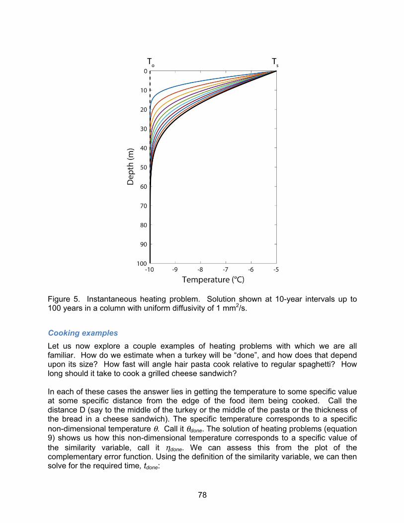
78

Figure 5. Instantaneous heating problem. Solution shown at 10-year intervals up to 100 years in a column with uniform diffusivity of 1 mm2/s.

Cooking examples Let us now explore a couple examples of heating problems with which we are all familiar. How do we estimate when a turkey will be “done”, and how does that depend upon its size? How fast will angle hair pasta cook relative to regular spaghetti? How long should it take to cook a grilled cheese sandwich? In each of these cases the answer lies in getting the temperature to some specific value at some specific distance from the edge of the food item being cooked. Call the distance D (say to the middle of the turkey or the middle of the pasta or the thickness of the bread in a cheese sandwich). The specific temperature corresponds to a specific non-dimensional temperature θ. Call it θdone. The solution of heating problems (equation 9) shows us how this non-dimensional temperature corresponds to a specific value of the similarity variable, call it ηdone. We can assess this from the plot of the complementary error function. Using the definition of the similarity variable, we can then solve for the required time, tdone:

79

tdone =

1κ

D2ηdone

⎛

⎝⎜⎞

⎠⎟

2

(8.17)

Without plugging in specific values, we can easily assess the sensitivity of the required cooking time to the size of the food item. If the bigger turkey is 50% bigger in radius, it will require 1.52 or about 2.5 times longer for the middle of the turkey to be at the required temperature. And if angel hair pasta is half the diameter as regular spaghetti, it will take a quarter of the time to cook. These are simple takeaway lessons from this kind of analysis.

Summary questions: Describe in words the physics behind why the thermal profile evolves as it does after the temperature at the surface drops or increases. Walk through the steps that Lord Kelvin used in estimating the age of the Earth from the thermal profile…Know the objections to it, what assumptions he made and what are better ones. Again, how are length and time scales related in diffusion problems… and why?

References Davies, G., 1999, Dynamic Earth: Plates, Plumes and Mantle Convection, Cambridge:

Cambridge University Press. Davies, G., Mantle Convection for Geologists England, P., P. Molnar, F. Richter, 2007, John Perry’s neglected critique of Kelvin’s age

for the Earth: A missed opportunity in geodynamics, GSA Today: 17(1), doi: 10.1130/GSAT01701A.1

Turcotte, D.L. and G. Schubert, Geodynamics, 3rd edition Examples of boundary layers in thermal problems, velocity fields, concentration fields heat flux through time also 1/sqrt(t) scale it first, using ΔT/δ, then do it formally using erf solution Examples of instantaneous heating problems: Heating Coffee cups, Grilled cheese sandwiches, and boiling potatoes Contact metamorphism

(note other metamorphic problems can be treated using steady solutions) Climate change signal (more on this later) Examples of instantaneous cooling problems: Other applications:

Cooling of lava flows – Steens mountain reversal story Freezing of a lake – Stefan problem, requires accounting for heat of fusion Abramov & Mojszis piece on early Earth thermal regime and life

Oceanic lithosphere, oceanic bathymetry (next time)

80

The lithosphere and a thermal boundary layer One of the classes of transient problems that we can work analytically is called “instantaneous warming or cooling of a half-space”. In general, the surface could be either warmed or cooled relative to the interior; the mathematical solution for the resulting wave of thermal disturbance progressing into the interior is the same. You can imagine that because this disturbance propagates into the interior, there must be some region near the boundary within which the temperature has changed “significantly” from its prior state. We call this region a “thermal boundary layer”. As we will see, the definition of “significant” change is somewhat arbitrary, but once we have defined it, the behavior of the boundary layer is quite understandable. Here I employ this notion to address a key element of the Earth – its lithosphere. We will see that the lithosphere is best thought of as a thermal boundary layer. At a mid-ocean spreading ridge, two lithospheric plates slide away in opposite directions at speeds of several cm/year. Mantle beneath the ridge rises to replace that lost, and in so doing experiences decompression melting. The basaltic melt rises to produce oceanic crust, solidifying either at the surface or in the subsurface. This basaltic oceanic crust is on the order of 5-7 km thick. But the plate is not the crust. The plate includes the crust, but is largely that portion of the upper mantle that is cool enough to behave as an elastic solid on geologic timescales. The word plate evokes something that does not flow; it is a rigid body. The distinction is one of material behavior, or rheology. The rheology of a substance is its response to forces (or more formally, to stresses, which are forces per unit area). An elastic rheology (the simplest solid) is one in which a finite strain of the material is produced by an imposed stress; the strain is recovered when the stress is released. In contrast a viscous rheology (the simplest fluid) is one in which the longer the stress is applied, the higher the strain. There is no single relationship between stress and strain. Instead, we find that the rate of strain is proportional to stress. Back to the lithosphere, we may think of these plates as being defined by a “rheological boundary layer”. In rocks, and for that matter in ice, we find that the rheology is critically dependent upon temperature. When either rock or ice is anywhere near its melting point, it behaves as a viscous material, while at much colder temperatures it behaves like an elastic solid. The cross-over temperature for mantle rock is sort of fuzzy, but call it 1200°C to 1300°C. That part of the upper mantle that is cooler than 1200°C will therefore behave as a solid on geologic timescales – this is the lithospheric “plate”. In assigning a thickness to the lithosphere, our task is now converted into determining the depth of the 1200°C isotherm. We have transformed the problem into a thermal problem. Beyond the region very close to the ridge, where groundwater circulation of fluids can extract heat efficiently from the thin cooling plate, the main means by which heat is transported within the lithosphere is conduction. The equations we have developed, in particular the diffusion equation, therefore capture the physics. The system is by no means steady, however, meaning that we cannot make the simplifying assumptions that allowed us to develop the equation for the geotherm. The problem is, however, much

81

like that involved in cooking problems, or in the warming of permafrost – only this time the temperature at the boundary has dropped rather than risen. Consider a column of crust and underlying upper mantle. This column is moving at half the spreading rate, but the entire column is moving. It is a solid. We can therefore think of the problem as being a 1D problem, in depth, as we ride along the spreading conveyor. At just before the clock starts, at time = 0-, the column is at the spreading ridge and is uniform in temperature. At time = 0, the top of the column is exposed to the base of the ocean, and thereafter this top surface is maintained at the temperature of the ocean floor. It IS the ocean floor. The column cools through time, and the depth to the 1200°C isotherm deepens. This is an instantaneous cooling problem, and is depicted in Figure 1 (after A&A chapter 3, Figure 4).

Figure 1. This is identical to Figure 1 in the last lecture, except that we are now specific about the temperatures at the surface. Physically, you should be able to see from the three profiles shown in the figure why the temperatures at any depth should change rapidly at first and then more slowly. Recall that the rate of cooling of an element of the material lying between the dashed lines is governed by the mismatch between the heat flowing out of the element and the heat flowing into it. The greater the mismatch, the faster the cooling. And the rate of heat flow by conduction is in turn governed by the gradient in temperature across the boundary. Turning to the math, recall how we defined the dimensionless variables θ and η to solve the diffusion equation for heating and cooling problems. For the cooling problem that is relevant to the lithosphere, the non-dimensional temperature is defined as

θ =

T −Ts

T0 −Ts

(9.1)

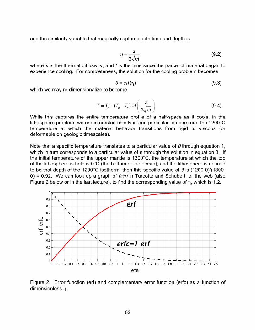
82

and the similarity variable that magically captures both time and depth is

η = z

2 κ t (9.2)

where κ is the thermal diffusivity, and t is the time since the parcel of material began to experience cooling. For completeness, the solution for the cooling problem becomes θ = erf (η) (9.3) which we may re-dimensionalize to become

T =Ts + (T0 −Ts )erf z

2 κ t

⎛⎝⎜

⎞⎠⎟

(9.4)

While this captures the entire temperature profile of a half-space as it cools, in the lithosphere problem, we are interested chiefly in one particular temperature, the 1200°C temperature at which the material behavior transitions from rigid to viscous (or deformable on geologic timescales). Note that a specific temperature translates to a particular value of θ through equation 1, which in turn corresponds to a particular value of η through the solution in equation 3. If the initial temperature of the upper mantle is 1300°C, the temperature at which the top of the lithosphere is held is 0°C (the bottom of the ocean), and the lithosphere is defined to be that depth of the 1200°C isotherm, then this specific value of θ is (1200-0)/(1300-0) = 0.92. We can look up a graph of θ(η) in Turcotte and Schubert, or the web (also Figure 2 below or in the last lecture), to find the corresponding value of η, which is 1.2.

Figure 2. Error function (erf) and complementary error function (erfc) as a function of dimensionless η.

83

Returning to the definition of the similarity variable in equation 2, we see that by setting η to 1.2, we may deduce the expected history of the thickness of the lithosphere, L, through

ηL = 1.2 =

L2 κ t

L = 2.4 κ t

(9.5)

where the bottom equation is a simple rewriting of the top. Note that the thickness of the lithosphere, L, goes simply as the square root of time. This by now should be familiar – in conduction problems, length scales go as square roots of timescales, whereas timescales go as squares of length scales. Given that plate speeds are pretty steady, we can transform time into distance from the spreading ridge through x = u1/2t, where u1/2 is the half spreading rate. We therefore predict that the profile of lithospheric thickness, L, across a spreading ocean basin is

L = ηLκ xu1/2

(9.6)

The lithosphere should thicken as the square root of distance from the spreading ridge. How would we check this? The figure below shows the bathymetry of two major ocean basins with distance from the mid-ocean spreading ridges.

Figure 3. Bathymetry in two ocean basins as a function of lithosphere age.

84

It has been argued that this bathymetric profile reflects the thickening of the lithosphere. The argument goes like this: Part 1 is that the lithosphere thickens with time and distance as we have just discussed, and as the square root of time in particular. Part 2 is that the profile of ocean-crust-lithosphere-mantle is in isostatic balance. By definition, the lithosphere is cooler than the mantle immediately below it (its mean temperature is about (1300-0)/2 ~ 650°C, which is therefore about 650°C cooler than the 1300°C mantle immediately beneath it). Part 3 acknowledges that cooler material is denser than hotter material. Isostatic compensation of this cooler denser lithosphere dictates that the thickness of low-density ocean be greater where the thickness of high-density lithosphere is greater. Hence the bathymetry should mimic the thickness profile of the lithosphere. The analysis of Parsons and Sclater (1977) has been updated by Stein and Stein (1992), but the essence remains: we can explain straight-forwardly the ocean basins of the planet, and hence the gross topography of 70% of the planet’s surface. Just to get specific and more quantitative, let us calculate the expected thickness of the lithosphere when the age of the plate is 60 million years. We have from equation 5 L = 2.4 κ t = 2.4 31* 60 *106 = 2.4 * 41km = 98km (9.7) The lithosphere should therefore be about 100 km thick at 60 Ma.

Figure 4. Schematic diagram of the relationship between lithospheric thickness and ocean bathymetry. (after A&A chapter 3, Figure 5) Let’s see how well we do in predicting how deep the ocean should be above a plate that thick. The isostatic problem is depicted in Figure 4. The pressures at points 1 and 2 must be equal to prevent flow of mantle in one or the other direction along the dashed line. Summing of pressures associated with the different materials with different thickness in each column yields an equation that can be algebraically manipulated to yield

85

D = L

ρL − ρm

ρm − ρw

⎡

⎣⎢

⎤

⎦⎥ (9.8)

where the subscripts m, w and L correspond to upper mantle, ocean water and lithosphere. Before we evaluate this, note that the depth of water below that of the spreading ridge should simply mimic the thickness of the lithosphere; in other words, the fraction in the brackets is simply a number. To evaluate this number we need to know the densities. That of the hot upper mantle is simply peridotite, and we are pretty safe in saying this is 3300 kg/m3. That of ocean water is 1030 kg/m3, which we can approximate as 1000 kg/m3. But what about lithosphere? Recall that the lithosphere is simply cooled upper mantle, so we have to address how the density of a material changes as we cool it. All materials contact as they cool, meaning you can fit more mass into the same volume, which is to say that their density must rise. But by how much? The densities are related through this simple linear relationship with temperature,

ρnew = ρold 1−αΔT( ) (9.9) where ΔT is the change in temperature (negative if cooled, positive if warmed), and α is a material property called the coefficient of thermal expansion. This coefficient is measured to be 1-3x10-5/°C for rock. We may now rewrite equation 8 as

D = Lρm(1+αΔT ) − ρm

ρm − ρw

⎡

⎣⎢

⎤

⎦⎥ = L

ρmαΔTρm − ρw

⎡

⎣⎢

⎤

⎦⎥ (9.10)

Using the densities of upper mantle and ocean above, 3x10-5/°C for the coefficient of thermal expansion, and ΔT=650°C, we find that D=0.03L; the excess water depth below the spreading center should be about 3% of the lithosphere thickness. Turning this on its head, the lithosphere thickness should be about 1/0.03 or 33 times that of the excess water depth. Going back to Figure 3, we see that at 60 Ma the excess water depth is about 3 km. The lithosphere should be about 3x33=99 km thick. Recall that our thermal calculation suggests that the lithosphere ought to be 100 km thick at 60 million years. We get the same answer (!) This means that not only can we explain the square root pattern of the ocean floor depths, but that we can do so quantitatively. This is one of the great triumphs of the plate tectonics model. It can explain 2/3 of the planet’s topography! Let me summarize. We can explain the square root of time dependence of the ocean bathymetry as a mirror of the square root of time thickening of the lithosphere. The lithosphere is therefore simply explained as a thermal boundary layer that grows in thickness with time and hence with distance from spreading centers. The droop of the seafloor is required to remain at isostatic balance. And the density difference between the hot upper mantle or asthenosphere beneath the plate and the lithosphere itself is simply calculated as a result of thermal contraction. In this calculation we have

86

appealed to a few material properties: the thermal diffusivity, the coefficient of thermal expansion, and densities of mantle and ocean. Knowledge of these simple properties allows us to explain the topography of 2/3 of the planet!

87

Advection

I introduce here a topic that many students find confusing. We have already talked about how heat can conduct in a solid, moving from hot to cold. And we have talked about radiation, transporting heat through translucent media. There is a third mechanism, called advection, that plays a major role in transporting heat in moving media, like water and air. Advection is the main means of transport of momentum and heat (and many other quantities) in the atmosphere and in rivers. It also provides an important analog for transport of any quantity in a moving medium. When the medium is in motion, there is a possibility that the temperature, which we can think of as the concentration of heat at a point, can change due to that motion. Whether this happens or not depends upon whether there is a gradient of the temperature as well, and in particular a gradient of temperature in the direction of motion. I will define advection as follows: Advection: The rate of change of some quantity due to material motion in the direction in which there is a gradient in the concentration of that quantity. Advection can be very efficient because the transport is accomplished by the fluid motion. The quantity is embedded in the fluid and moves with it. The process does not depend upon the passage of heat (or any other quantity) by random molecular motion, as in conduction of heat, but involves the bulk motion of the fluid. I use this discussion of advection as an excuse to introduce two other topics. The role of advection can be illuminated by comparing the same phenomenon from two points of view. But let us begin. Consider a herd of sheep on a hillslope. The herd of sheep is being watched by two shepherds. Shepherd 1, call him Elmer, is riding his horse along with the herd, while the other, shepherd 2, call him Clovis, is taking a break on a hillside across the stream, and is watching as the herd moves left to right across the opposite hillside (Figure 1). Sheep always move left to right. Let us say that the quantity of concern is the concentration of sheep, the number of sheep per unit area, say a hectare (100m x 100m). The sheep have arranged themselves into a band with a sharply defined leading edge, defined by a couple bellwethers and the sheep who follow closely on their heels, and a more diffuse straggelly back end with the slowpokes, the injured, and the renegades, who if it were not for the trusty sheepdog would be lost entirely. What does this look like to Elmer, the shepherd traveling with the band? It looks like a steady pattern with not much change as he slowly rides along with the band. Looking ahead he sees the strongly defined front, and behind he sees the diffuse trailing edge to the band. It looks the same another half an hour later, on a different hillside, the entire herd having moved hundreds of meters. But what does this look like to Clovis, the shepherd taking a break? Looking across the creek, he sees anything but a steady pattern.

88

Staring at the same segment of hillside he has in his field of view, he sees first the arrival of the sharply defined front end of the herd, then the high concentration of the middle of the band, with Elmer at the edge of it, and finally he sees the diffuse tail go by, after which the concentration of sheep on this hillside returns to zero. From his perspective there has been a temporal pattern of sheep concentration, while for his buddy moving with the sheep the pattern was steady, not changing in time. What is seen depends upon the point of view. These points of view are the end-member cases, one still, the other traveling with the medium. These have names: that traveling with the medium is the Lagrangian point of view, while that pinned down at a point is the Eulerian point of view. (Joseph Louis Lagrange (1736-1813) was an Italian-born mathematician and astronomer, teacher of Fourier and Poisson; Leonhard Euler (1707-1783) was a prolific Swiss-born mathematician and physicist who spent most of his life in Germany and Russia.) In order to go back and forth between these points of view, which in the end must describe the same system, we need advective terms in the equation describing the system. But let me do this graphically first.

Figure 1. Lagrangian and Eulerian points of view and advection. Top: pattern of sheep on a hillside traveling left to right seen at an instant. Middle (Lagrangian point of view): the pattern of sheep concentration plotted as a function of distance along the hillside,

89

with the sharp leading edge and diffuse tail. Bottom (Eulerian point of view): pattern of sheep concentration as a function of time as seen by an observer fixed in space. At an early time, t1, the concentration of sheep steeply rises (dC/dt>0) as the tightly bunched leading edge of the band comes by the view. At a later time, t2, the concentration of sheep slowly falls (dC/dt<0) as the diffuse tail rambles by. (Can you find the black sheep?) We would like to be able to get back and forth between these two points of view. After all, they describe the same system. Clearly we need some mathematical mechanism that involves derivatives in time and derivatives in space. Let us get precise. To describe the Lagrangian point of view, we must define a derivative following along with the medium. This is called the “substantial derivative”, or the “derivative following the fluid” or medium. It is denoted D/Dt, with a big D instead of a partial. In the case I have illustrated, the rate of change of sheep concentration following along with the herd, as seen by the herder embedded in the herd, is zero. He (or she) sees no change in the pattern through time; it would always look like that shown in the top graph; DC/Dt = 0, C being the concentration of sheep. The herder across the creek, however, is fixed in space. In his fixed field of view, he sees a temporal pattern of concentration, shown in the bottom diagram. He sees temporal changes while fixed in space. We use the partial derivative to denote this, or ∂C / ∂ t . This means formally that, all other variables fixed (here we only had one spatial variable, x), this is the pattern seen. It is only changing in time. So how do we get between these points of view? It comes through the full definition of the substantial derivative. Let me define it first, and then turn back to the sheep. The substantial derivative of a hypothetical quantity, which I have called A, is:

DADt

= ∂A∂ t

+ u∂A∂ x

+v∂A∂y

+w∂A∂z

(10.1)

Here u is the speed in the direction x, v that in the direction y and w that in the direction z. Translating to words, the rate of change following the medium, the substantial derivative, depends upon the rate of change at a fixed point plus the rate of change caused by motion in any direction in which there is a gradient of the concentration. These last 3 terms are called the advective terms. In our case, the variable of concern is the concentration of sheep, C, we have only one spatial dimension, x, and the speed of the herd moving in that direction is u. For the case involving the sheep, the substantial derivative then becomes:

DCDt

= ∂C∂ t

+ u∂C∂ x

(10.2)

In the scenario I have described, the substantial derivative is zero. There is no change following along with the herd, from Elmer’s point of view. We can now translate between what Elmer sees and what Clovis sees by setting DC/Dt=0:

90

∂C∂ t

= −u∂C∂ x

(10.3)

Does this work? Turning back to the figure, focus on the two times, t1 and t2. In the early time, the rate of change of sheep concentration with time is positive and high. It corresponds to the passage of the sharply defined front end of the band of sheep, with a strong negative concentration gradient, passing the site at a rate u. C changes because there is motion, u, in the direction in which there is a gradient, x. The minus sign assures us that concentration increases when negative concentration gradients advect by. Consider now the later time. Motion is in the same direction at the same speed, but this time the concentration gradient is positive. The negative sign assures that the concentration seen at the fixed site now declines as the pattern with a positive concentration gradient passes by. Consider a different problem, adapted from the one I originally heard (from JD Smith) to illustrate the concepts of advection and the substantial derivative. Imagine that you are a bug on a leaf, floating steadily northward in the ocean, having been delivered to the ocean from a river draining the cloud forest of Costa Rica. What temperature history might you record in your bug-sized thermometer? You are traveling with the medium, here seawater, so any changes you experience will involve the substantial derivative of temperature. This will include two kinds of change, one associated with temporal changes at any fixed point (say associated with daily oscillations in temperature), and the other with the fact that you are in motion in the direction in which there are gradients in temperature (associated with latitudes). The equation for the rate of change of temperature will be

DTDt

= ∂T∂t

+ u ∂T∂x

(10.4)

Here the 1st term on the right hand side represents the rate of change at a point (daily cycle) and the 2nd term represents the change associated with northward motion (defining x northward, and again u the component of velocity in the x direction). The first term will therefore rapidly vary with the daily temperature cycle. This oscillation will be embedded on a slow decline represented by the second term, as you the bug slowly advect into colder climates. I have attempted to capture this in Figure 2.

91

Figure 2. Temperature history recorded by a bug on a leaf floating northward from Costa Rica. The oscillations reflect the daily cycle of temperatures. The net cooling reflects advection into colder climates. Let us examine a couple more relevant thermal examples. In the first, imagine a site on a polar glacier in which there is no melting in the summer, and only slow net accumulation, at a rate b. If the ice were not in motion, the temperature profile would simply be a geotherm, reflecting steady operation of the conduction process, with a uniform gradient set by the heat flux and the thermal conductivity of the ice, Q/k. The net accumulation slowly buries a parcel of ice, giving it a velocity that transports heat in the direction of a temperature gradient, from the relatively cold surface downward. The full equation for the evolution of the temperature, ignoring sources of heat, is then

DTDt

= ∂T∂t

+ b ∂T∂z

=κ ∂ 2T∂z2

(10.5)

This differs from that presented in the discussion of permafrost in that it includes the second term on the left, representing downward advection of ice. There is advection because there is motion in the direction of a temperature gradient. A perfectly analogous situation exists when we consider the temperature profile we might expect in a landscape that is steadily eroding. This is analogous to the ablation area of a glacier, in which the surface is being brought closer and closer to a parcel of ice at depth. These problems involving a diffusive system in the face of motion of the medium in which diffusion is occurring can display a range of behaviors that depend upon the relative importance of the two processes of diffusion and advection. We can get formal

92

about defining which dominates by evaluating the relative importance of the mathematical terms in the master equation. Let us do this formally. Consider the heat equation that includes advection

∂T∂ t

=κ ∂ 2T∂z2 +w ∂T

∂z (10.6)

We now use a trick to non-dimensionalize this equation by appealing to the scales of each of the terms. In a way we are simply normalizing the length and time variables by relevant scales. Specifically, let’s say that the depths z can go form 0 to L. Maybe L is the thickness of ice, for example. If we construct a new dimensionless variable z’=z/L, it will only range from 0 to 1. We could also say T’=T/To. If we re-write the heat equation in these new variables, it becomes

∂(T 'To )∂ t

=κ∂ 2(T 'To )∂(z 'L)2 +w

∂(T 'To )∂(z 'L)

(10.7)

Separating out the scales from each term gives

To

∂T '∂ t

=κTo

L2

∂ 2T '∂z '2

+wTo

L∂T '∂z '

(10.8)

Now dividing by the scales in front of the diffusion term yields:

L2

κ t⎛⎝⎜

⎞⎠⎟∂T '∂ t

= ∂ 2T '∂z '2

+ wLκ

⎛⎝⎜

⎞⎠⎟∂T '∂z '

(10.9)

The collections of constants in front of each term (in parentheses) are all dimensionless. Note that there is an invisible 1 in front of the diffusion term. The term in front of the temperature gradient we name the Peclet number (Pe):

Pe = wL

κ (10.10)

This represents the relative importance of advection to diffusion in the particular problem at hand. Therefore, when Pe>>1, advection dominates, and we may therefore ignore the diffusion term altogether, whereas if Pe<<1, the advection term may be ignored. This is a powerful way to reduce the complexity of a problem. Let us now work a couple examples.

93

Temperature profiles in polar glaciers In many glaciers around the world, the temperature may be safely assumed to be both uniform, and very close to the pressure melting point of ice. However, if the mean annual surface temperatures are way below freezing, and the melting of ice at the surface and its percolation to depths where it refreezes - thereby depositing its latent heat – are insufficient to homogenize the temperatures, the temperatures are governed by a combination of conduction (hence diffusion) and advection of heat. The problem set up is illustrated in Figure 2. Consider a steady glacier, in which its shape is unchanging from year to year. We have two cases, one in which the ice is moving downward from one year to the next, and one in which ice at the surface is moving upward from one year to the next. The former occurs in the accumulation zone, where net accumulation of new snow must be accommodated, whereas the latter occurs in the ablation zone, where net loss of ice from the surface requires that ice thicken there. (See discussion in both Cuffey and Paterson (2010) and in Hooke (2005) of the expected temperature profiles in both accumulation and ablation areas of glaciers.)

Figure 3. Schematic diagram for temperature profile at two sites on a glacier. A) accumulation zone, and B) ablation zone. The ice has thickness H, and a local mass balance b (which is positive in the accumulation area, and negative in the ablation area). Climate imposes the surface temperature Ts and the tectonic setting imposes geothermal heat flux and hence the temperature gradient at the base, dT/dz. Vertical speed structure w(z) is assumed to ramp linearly from zero at the bed to the surface value (see text). The relevant heat equation includes both diffusive and advective terms. Here we just focus on the vertical component of motion and of heat flow, knowing that this is a simplification:

94

∂T∂t

=κ ∂2T∂z2 −w ∂T

∂z (10.11)

where w is the component of ice velocity that is vertical. In steady state we may ignore the left hand side of the equation. To proceed, we must specify boundary conditions, or what happens at the top and bottom of the ice. At the bottom, the temperature structure is required to have the proper gradient to pass the geothermal heat, hence dT/dz=-Qm/k at z=0, where k is the thermal conductivity and Qm is the mantle heat flux. At the top of the ice, the temperature is the surface temperature Ts. The velocity structure requires that w=0 at the bed (z=0) (we assume that ice is still well below the pressure melting point there) and must equal the annual net balance, b, at the surface, (where z=H). We assume the simplest case in which the vertical speed linearly changes from the bed to the surface, in other words,

w = b z

H (10.12)

We may then arrive at a solution for the heat equation of the form (Cuffey and Paterson, 2010, eq. 9.16):

T =To +

dTdz z=0

exp(−z2 / z*2)dz

0

z

∫ (10.13)

where To is the basal temperature and

z* =

2κHb

(10.14)

The resulting solution may be attained for the case in which b>0:

T =Ts +

z* π2

dTdz z=0

erf (z / z* )− erf (H / z* )⎡⎣ ⎤⎦ (10.15)

The solution is plotted in Figure 4 for a range of conditions, each situation characterized by a particular Peclet number, Pe=bH/κ. Formally, only when b>0 is this called a Peclet number. It is called in the glaciological community the advection parameter, γ, which can range from >0 through 0 to <0 (See Figure 3).

γ = bH

κ (10.16)

95

Figure 4. Temperature profiles in a glacier in the face of vertical advection of the ice, either upward (b<0) in the ablation zone, or downward (b>0) in the accumulation zone. For the particular case shown, the surface temperature is set to -30°C, and the basal temperature gradient to -25°C/km (negative since z is taken positive upward). We should test this solution to make sure it makes sense. For example, in the case in which advection is turned off entirely (b=0, hence γ =0), we expect to recover the steady geotherm, a linear profile with slope Qm/k. Indeed this is the case. (Prove it: when z=0 in equation 13, the argument of the integral becomes 1 and upon integration is simply z. Hence the equation becomes that for the geotherm.) We also expect that the temperature gradient at the base of the ice is the same in all cases, in order to pass the geothermal heat upward into the ice. That too is clearly seen in the plot. Downward advection of cold ice from the surface occurs homogenizes the temperature profile for high accumulation rates (high γ). It is also clear on this plot that in the ablation zone of polar glaciers, the ablation rate cannot exceed a particular value before the temperature at the base of the ice reaches its pressure melting point. Here we have used H=500 m, and the last case shown (γ =-4) corresponds to b=-0.25 m/yr. Ablation rates exceeding this will result in basal ice at the pressure melting point. Typical values of the advection parameter for the accumulation zone in Greenland, using H=3 km, b=0.25 m/yr, are γ=21. Typical values for the accumulation zone in central East Antarctica, using H=4 km, b=0.025 m/yr, are γ =2.8. The bottom line is that

96

the geotherm is not greatly affected by advection in Antarctica, whereas in Greenland advection dominates.

Warped geotherms in active orogens Finally, I note that the same physics pertains to a package of rock that is being uplifted within an active orogeny. Motivations for studying the thermal structure of an orogeny include both the dependence of the material properties on the temperature of the rock (its rheology), and interpretation of thermochronometers such as fission tracks and He concentrations (e.g., Reiners and Brandon, 2006). These encode information about the thermal history, in particular passage through partial annealing zones and closure temperatures. In order to employ this thermal information to deduce patterns and rates of exhumation or erosion, one must know the dependence of temperature on depth. Consider a steady orogeny, in which the rate of rock uplift equals the rate of erosion. The rock simply wafts upward through the orogeny. The rock uplift rate is uniform through the orogen, entering at its base at a depth L, and leaving through the top by erosion of the rock, all at a speed w. The temperature at the base of the orogeny is assumed fixed at Tb, and the temperature at the surface is set to Ts. Under these conditions, the solution to the diffusion-advection equation becomes

T =Ts + (TL −Ts ) 1− e−wz/κ

1− e−wL/κ

⎡

⎣⎢

⎤

⎦⎥ (10.17)

(Reiners and Brandon, 2006, eqn. 8a, although the 1 is missing in the denominator in their equation). For conditions appropriate for the northern Apennine orogen in Italy, this is plotted in Figure 5 for a range of plausible rock uplift rates.

97

Figure 5. Steady temperature profiles for a variety of erosion rates (= rock uplift rates) from 0 to 10 mm/yr at 1 mm/yr intervals. (after Reiners and Brandon, 2006, Figure 3). Just as in the ablation zone of a glacier, the warping of the temperature profiles increases as the uplift rate increases, reflecting the increasing role of advection in governing the shape of the profile. And again, the cases can be discriminated using the relevant Peclet number or advection parameter, here Pe=wH/κ.

Summary We have seen that this other means of transporting heat, by motion of the medium in which the heat is embedded, can be important in many geologic cases. Just as diffusion terms are always second derivatives of some property with respect to distance, so too do advection terms always have the same look. They are always the products of a component of velocity with a gradient of some property (here temperature) in the same direction. The relative importance of the advection and diffusion in transporting heat (or any other quantity in the material) can be captured by a non-dimensional collection of constants that we call the Peclet number. We have explored a two cases in which advection is important. In both the glacial and orogeny cases, the temperature profiles can be warped significantly. We will see later that the resulting temperature structure can strongly influence the rheology of the material.

References Cuffey, K., and W.S.B. Paterson, 2010, The Physics of Glaciers, 4th edition

98

Reiners, P.W. and M.T. Brandon, 2006, Using thermochronology to understand orogenic erosion, Annu. Rev. Earth Planet. Sci., 34:419–66, doi: 10.1146/ annurev.earth.34.031405.125202

Turcotte, D., and G. Schubert, 2014, Geodynamics, 4th edition. Cambridge: Cambridge

University Press. Note: The front end of this chapter/lecture was presented as introductory material in the

Little Book of Geomorphology.

99