University of New MexicoUNM Digital Repository

Mechanical Engineering ETDs Engineering ETDs

2-1-2016

Geolocation of Utility Assets UsingOmnidirectional Ground-Based PhotographicImageryHisham Tariq

Follow this and additional works at: https://digitalrepository.unm.edu/me_etds

This Thesis is brought to you for free and open access by the Engineering ETDs at UNM Digital Repository. It has been accepted for inclusion inMechanical Engineering ETDs by an authorized administrator of UNM Digital Repository. For more information, please contact disc@unm.edu.

Recommended CitationTariq, Hisham. "Geolocation of Utility Assets Using Omnidirectional Ground-Based Photographic Imagery." (2016).https://digitalrepository.unm.edu/me_etds/52

i

Hisham Tariq Candidate

Mechanical Engineering

Department

This thesis is approved, and it is acceptable in quality and form for publication:

Approved by the Thesis Committee:

Andrea Mammoli, Chairperson

Thomas Caudell

Peter Vorobief

ii

Geolocation of Utility Assets Using

Omnidirectional Ground-Based

Photographic Imagery

by

HISHAM TARIQ

B.E., NED UNIVERSITY OF ENGINEERING AND

TECHNOLOGY

THESIS

Submitted in Partial Fulfillment of the

Requirements for the Degree of

Master of Science

Mechanical Engineering

The University of New Mexico

Albuquerque, New Mexico

December, 2015

iii

ACKNOWLEDGMENTS

Firstly, I would like to express my sincere gratitude to my advisor Dr. Andrea

Mammoli for the continuous support of my M.S. study and related research, for his

patience, motivation, and immense knowledge. His guidance helped me in all the

time of research and writing of this thesis. I could not have imagined having a

better advisor and mentor for my M.S. study. He supported me throughout not just

in my thesis but my entire graduate career. Also, I would like to thank him for

encouraging me and pushing me to produce quality work. His teachings and

guidance will remain with me as I continue my career.

I also thank my committee members, Dr. Thomas Caudell and Dr. Peter Vorobief,

for their recommendations pertaining to this study and for their willingness to

serve on my committee and share their knowledge and expertise. I like to thank

them for their insightful comments and encouragement, but also for the hard

question which incented me to widen my research from various perspectives.

And finally to my parents, especially my mom who gave me immeasurable

supports over the years and pushed me to do my best.

iv

Geolocation of Utility Assets Using

Omnidirectional Ground-Based

Photographic Imagery

by

HISHAM TARIQ

B.E., Mechanical Engineering, NED University Of Engineering and

Technology, 2013

M.S., Mechanical Engineering, University of New Mexico, 2015

ABSTRACT

A process for using ground-based photographic imagery to detect and locate

power distribution assets is presented. The primary feature of the system

presented here is it's very low cost compared to more traditional inspection

methods because the process takes place entirely in virtual space. Specifically,

the system can locate assets with a precision comparable to typical GPS units

used for similar purposes, and can readily identify utility assets, for example,

transformers, if appropriate training data are provided. Further human

intervention would only be necessary in a small fraction of cases, where very

high uncertainty is flagged by the system. The feasibility of the process is

demonstrated here, and a path to full integration is presented.

v

Table of Contents

List of Figures ............................................................................................................................................... vii

List of Tables ................................................................................................................................................. x

1 Introduction ........................................................................................................................................... 1

1.1 Motivation and Approach .............................................................................................................. 4

2 Literature Review .................................................................................................................................. 7

2.1 Transmission and Distribution ....................................................................................................... 7

2.2 Smart Grid and GIS ....................................................................................................................... 7

2.3 GIS Data through Panoramic images ........................................................................................... 9

2.4 Google Street View ..................................................................................................................... 11

3 Image Acquisition ............................................................................................................................... 14

3.1 Google Street View Parameters.................................................................................................. 15

3.2 Google Street View Usage Limits ............................................................................................... 18

3.3 Concept ....................................................................................................................................... 20

3.3.1 External Script Files ............................................................................................................ 23

3.3.2 Code Algorithm .................................................................................................................... 25

4 Large-Scale Image Acquisition ........................................................................................................... 28

4.1 Steps Leading to Image Acquisition ............................................................................................ 33

4.2 Database Creation for Image Acquisition ................................................................................... 33

4.2.1 Sequence of Operation for Database Creation ................................................................... 33

4.2.2 Building Tables in Database ............................................................................................... 35

vi

4.2.3 Code Algorithms: ................................................................................................................. 39

4.3 Text File Generation .................................................................................................................... 50

4.3.1 Index.php ............................................................................................................................. 50

4.3.2 Generate-txt.php ................................................................................................................. 52

4.4 Image Acquisition ........................................................................................................................ 56

4.4.1 Poly-Map.html ..................................................................................................................... 57

4.4.2 Image-Acq.html ................................................................................................................... 60

5 Asset Geo-Location and Error Analysis ............................................................................................. 64

5.1 Detection of Poles ....................................................................................................................... 64

5.2 Geolocation of Pole ..................................................................................................................... 70

5.3 Errors cause and Analysis: ......................................................................................................... 72

5.4 Clustering .................................................................................................................................... 82

6 Conclusion .......................................................................................................................................... 87

6.1 Results of the study ..................................................................................................................... 87

6.2 Future Research ......................................................................................................................... 87

Appendices ................................................................................................................................................. 90

References ................................................................................................................................................ 121

vii

List of Figures

Figure 1. Installed transmission line length by region [1] ................................................. 2

Figure 2. Scope of project .............................................................................................. 5

Figure 3. Two user-specified cross-slits cameras, represented by slit pairs WX-g and

YZ-b, partitions the camera path WXYZ into three sections. The plane P1, formed by

the slit g and point X, represents the rightmost column of pixels in cross-slits camera

WX-g and their associated ray directions. Similarly, P2 is the plane formed by slit b and

point Y. These two planes P1 and P2 intersect in line r, which becomes the interpolating

slit. The XY-r cross-slits pair becomes the interpolating camera. Note that the

interpolating camera has the same ray directions on its edges as its neighboring

cameras. This ensures that the generated image contains no discontinuities [8] .......... 10

Figure 4. Google Street View R7 camera ...................................................................... 12

Figure 5. Route covering part of Corrales road, NM for image acquisition .................... 15

Figure 7. Different pitch angles ..................................................................................... 16

Figure 8. Zoom levels available in Google Street View ................................................. 18

Figure 8. Markers showing Street View car‟s position from where images were captured

...................................................................................................................................... 20

Figure 10. Images returned at every location of Google Street View car ...................... 21

Figure 11. Headings of the images at each car ............................................................. 22

Figure 11. Stitched panoramic image ............................................................................ 23

Figure 12. Central Ave route, Albuquerque ................................................................... 28

Figure 13. Central Ave route passing through waypoint ................................................ 29

viii

Figure 15. Fetching Sequence for Database tables ...................................................... 31

Figure 16. Web pages based on internal database ....................................................... 32

Figure 16. Basic structure of large-scale image acquisition application ........................ 33

Figure 17. Database creation ........................................................................................ 34

Figure 18. Accessing database through CMD ............................................................... 35

Figure 20. Code Execution Sequence for Address Database Tables Creation ............. 36

Figure 20. Sample address text file ............................................................................... 37

Figure 21. State‟s table ................................................................................................. 41

Figure 22. County‟s table .............................................................................................. 45

Figure 23. Zip code‟s table ............................................................................................ 49

Figure 24. Map showing routes of NM 87048 ................................................................ 59

Figure 25. Pole recognition ........................................................................................... 64

Figure 26. Transformer recognition ............................................................................... 65

Figure 27. Manual process of clicking on pole‟s position ............................................... 66

Figure 28. Acquisition of four images at a geographical location, corresponding to a 90º

field of view in the direction of each corner of the car.................................................... 67

Figure 29. Panorama showing the angular position of a pole with respect to the North.67

Figure 30. The intersection of lines in the direction of features detected in two

panoramas, each associated with a vehicle-mounted camera position. Each intersection

is a possible geo-location of a pole. .............................................................................. 71

Figure 31. Intersection results ....................................................................................... 72

Figure 33. Combined errors .......................................................................................... 74

ix

Figure 33. Errors in position of individual point .............................................................. 75

Figure 34. Errors in angle of individual point ................................................................. 76

Figure 36. Errors in angle of both points ....................................................................... 77

Figure 36. Histogram Plot .............................................................................................. 78

Figure 37. Contour Plot ................................................................................................. 79

Figure 38. Error in angle from pixel-based heading estimate ........................................ 80

Figure 39. Uncorrected Markers Position ...................................................................... 81

Figure 40. Corrected Markers Position .......................................................................... 82

Figure 41. Inter-particle attractive force ......................................................................... 83

Figure 42. Clustering algorithm: the form of the inter-particle force is shown in the inset.

Initial clustered pole locations from multiple triangulations (green squares) coalesce into

a single point for each cluster (triangles). The purple line indicates the camera vehicle

path, the crosses the location of panorama image collection. ....................................... 84

Figure 43. Examples of the location of poles using multiple triangulations from

omnidirectional image panoramas. In the majority of cases, the triangulated location is

within one meter of the actual pole position. ................................................................. 85

Figure 44. Clustering Result .......................................................................................... 85

Figure 45. Consumer-Grade GPS Result ...................................................................... 86

x

List of Tables

Table 1. Zoom levels and corresponding field of view ................................................... 17

Table 2. Google Street View requests limitations [15] ................................................... 19

Table 3. Google Street View map loads quantity pricing [15] ........................................ 19

xi

Glossary

AC Alternating Current

API Application Programming Interface

CMD Command Prompt

EPRI Electric Power Research Institute

FOV Field of View

GIS Geographic Information System

GPS Global Positioning System

HTML Hyper Text Markup Language

HVAC Heating, Ventilation and Air conditioning

PHP Personal Home Page (Server-side scripting language)

PV Photo Voltaic

PX Pixels

R2, 5 or 7 Rosettes 2, 5 or 7

SQL Structured Query Language

T & D Transmission and Distribution

URL Uniform Resource Locator

RR, RL, FL, FR Rear Right, Rear Left, Front Left, Front Right

1

1 Introduction

Electricity Generation occurs in Power Generation Plants located in far off areas. The

electricity produced reaches the consumer through a Network of Transmission and

Distribution (T&D) Lines. These T&D lines are spread all over the US, present even in

remote areas, and provide consumers with Electric energy. In 2011, the total installed

T&D lines length reached 69.5 million kilometers; in 2016, that figure will reach 74.2

million kilometers [1].

Although they are part of the same network, Transmission lines and Distribution lines

can be easily differentiated. Transmission lines, which can be hung overhead or

underground, are operated at relatively high voltages, they transmit large quantities of

power, and they transmit the power over large distances. Distribution Lines, however,

includes the lines that are connected to, poles, transformers and other equipment

needed to deliver electric power to the customer at the required voltages.

Transmission and distribution lines can be underground or overhead, but due to the

cost, maintenance and transmission losses in underground Lines esp. for high voltage

transmission, Overhead Lines are preferred. It is estimated that in the US, the

2

percentage of existing underground transmission lines out of the total transmission lines

is around 0.5-0.6 percent [2].

Figure 1. Installed transmission line length by region [1]

The current grid layout in the US is designed to support uni-directional flow only and has

been in use for over a century now [3]. More Complex systems are needed to cope with

the growth of societies, power requirements and sustainable energy areas. There is a

need for smart grid system and the intelligence of smart grid relies heavily on GIS data

3

[4]. All T&D lines have Geographic Information System (GIS) data associated with them.

This data includes useful information like the location of poles and transformers linked

to these lines.

Utility companies, in majority cases, maintain a GIS field data for various purposes.

However, their data is not reliable and the errors in readings are also not consistent.

This variance in the data is because utility companies have traditionally used

technicians to ride out T&D lines to determine reliability issues and to update related

systems with most current field information. This task typically requires two people to

scan the line. While one drives the vehicle, the other person documents the findings.

Because this work is usually distributed among teams, and also requires several years

to complete, in which these team members may also change, the results and

subsequent errors vary.

Advances have been made in the inspection processes; such as line robots. These

advances, however, are targeted and limited to transmission applications. While

distribution lines represent over 90% of the total lines length [1], their economic

significance per unit length is much smaller than for transmission lines. Therefore,

inspection of transmission infrastructure is essential in comparison to distribution lines.

Nevertheless, the performance of electricity grid hinges on the reliability of distribution

infrastructure. Moreover, the importance of the distribution system will increase as a

result of the increasing penetration of distributed resources such as rooftop PV. Hence,

4

there is a need for a low cost, accurate, and easily adaptable inspection tool for

distribution applications.

1.1 Motivation and Approach

A collection of utility poles field data is a tedious process. Also, the current method of

measurements, to go physically for each utility pole and gather data associated with the

pole, costs both time and money. Typically, data related with utility poles includes

images of the pole, geo-locations, distances between poles, pole and attachment

heights.

To improve this process and make it fast and economical, work has been done in this

project on the idea of remote capturing of pole related data. This method will save time,

and subsequently the cost, and has an added advantage of measuring reliable field

data.

Most of the distribution infrastructure is located near the roads for accessibility reasons.

Ground-based imagery databases, notably Google Street View, are available for the

bulk of the road system in the United States and other industrialized countries.

Mimicking the activity of utility technicians who go to the field, take images of poles and

other related data, a “virtual drive-by” is established, which is an automated system for

extracting images of a particular location available from Google Street View and later

5

on, these images can be processed for information on power distribution assets that are

embedded in imagery, including poles, lines, transformers and capacitor banks.

In this study, the groundwork for implementing a system that automatically inspects,

maps and categorizes distribution assets that are visible in ground-based imagery, is

performed.

There are three primary components of the framework, as illustrated schematically in

Figure 2: (1) automated acquisition of relevant ground-based imagery; (2) automated

Figure 2. Scope of project

Automated Acquisition of

Ground Based Imagery

Chapter 3 & 4

Automated Recognition of

Distribution Assets

Chapter 5

Geographical Location of

Utility Asset

Chapter 5

6

recognition of distribution assets from an image; (3) geographic location of the assets.

In the rest of the report, a description of these components is given. The accuracy of the

results is then discussed, followed by the outline of component integration needed for a

fully automated system.

7

2 Literature Review

2.1 Transmission and Distribution

There is continuous development in Transmission and Distribution (T&D) network of

electricity worldwide and this trend will continue with an increase in human population

and economic development.

Grid stability and reliability has driven new investment and overall spending in the T&D

markets with fewer major outages occurring in recent years. Despite a strong focus on

current grid infrastructure renewal, there has also been a significant expansion of the

grid network. To fulfill needs for ever expanding the network and accommodating power

generated through alternative means, a smart grid is needed.

2.2 Smart Grid and GIS

The smart grid system is dramatically changing the way electrical energy is delivered.

What has historically been a uni-directional flow of energy from power plant to

consumer is now increasingly paralleled with a bidirectional communication network to

optimize the use and flow of electricity [5].

Smart grid systems rely heavily on geospatial data in order to monitor assets and to

maintain accurate “as-designed” and “as-operated” models of the distribution system.

Consequently, as the smart grid model matures, and complexity will increase, the

availability and integrity of GIS data are becoming more imperative to augment [4].

8

The quality of GIS data has become increasingly important as the smart grid matures.

EPRI [5] undertook surveys of member utilities in 2012 to understand the costs

experienced by utilities due to unreliable GIS data. Utilities continuously struggle with

the quality of geospatial information system (GIS) data. With the advent of the Smart

Grid and advanced metering infrastructure, utilities are facing increased pressure to

resolve data quality issues.

GIS quality issues are primarily related to [5]:

Gaps, e.g. certain key information is missing;

Redundancies with other systems, e.g. data are captured in many systems and it

is inconsistent or requires duplicate data entry to update;

Inaccuracies with the field, e.g. GIS data exists but does not represent the actual

system in the field;

Inaccurate or unavailable land-base, e.g. Depending on its source, varying

degrees of accuracy of land-based data;

Customer to transformer connectivity by phase is in doubt.

Despite the importance of GIS data, electric utilities have not invested significantly in its

improvement due to the inability to cost-justify the effort [5].

9

2.3 GIS Data through Panoramic images

Utilities are photographed, in most cases unintentionally, in Ground-based imagery

along with various other landmarks. If utilities are located in them, these images can be

effectively utilized to obtain their GIS data. To improve accuracy, a multi-perspective

image is used. A multi-perspective image is in fact multiple views of a single scene from

different perspectives. In more common terms, they are called Panoramic Images.

Multi-perspective images generated from a collection of photographs or a video stream

can be used to effectively summarize long, roughly planar scenes such as city streets.

The final image will span a larger field of view than any single input image [6]. There are

several approaches for creating a multi-perspective image.

One possible approach to depicting the eye level urban fabric is to use a wide angle or

omnidirectional views around a single viewpoint. Omnidirectional camera [7] provides a

possible optical solution for capturing such views [8]. An omnidirectional camera is a

camera with a 360-degree field of view in the horizontal plane, or with a visual field that

covers (approximately) the entire sphere

Photo-mosaicking (the alignment and blending of multiple overlapping photographs) is

an alternative approach for creating a wide field of view images. These mosaics can be

made by capturing a part of the scene surrounding a single point by rotating a camera

around its optical center [9].

10

Another possible approach is to use pushbroom [10] or cross-slits imaging [11]. A

pushbroom image is an image that is perspective in one direction (e.g., vertically) and

orthographic in the other while a cross-slits image is an image which is perspective in

one direction but is the perspective from a different location in the other direction.

Google‟s ground based-imagery tool, Street View, uses an interactive system as shown

in Figure 3. Google Street View system visualizes urban landscapes using a blend of

adjacent cross-slits images.

Figure 3. Two user-specified cross-slits cameras, represented by slit pairs WX-g and YZ-b, partitions the camera path WXYZ into three sections. The plane P1, formed by the slit g and point X, represents the rightmost column of pixels in cross-slits camera WX-g and their associated ray directions. Similarly, P2 is the plane formed by slit b and point Y. These two planes P1 and P2 intersect in line r, which becomes the interpolating slit. The XY-r cross-slits pair becomes the interpolating camera. Note that the interpolating camera has the same ray directions on its edges as its neighboring cameras. This ensures that the generated image contains no discontinuities [8]

11

2.4 Google Street View

Google Street View was launched in 2007. Google Street View displays panoramas

of stitched images. Most photography is carried out by car, but some inaccessible areas

are covered by other means such as trekkers, tricycles, boats and on foot.

The initial car design of Google Street View included a side- and front-facing laser

scanner, two high-speed video cameras, eight high-resolution cameras in a rosette (R)

configuration, and a rack of computers recording data to an array of 20 hard drives at

500 Mbytes per second. The car also included special shock absorbers and a heavy-

duty alternator from a fire truck. The third generation of vehicles had a low-resolution

camera connected to a standard desktop PC with a single hard drive. These vehicles

were quite successful, recording a vast amount of imagery in the US and enabling

international expansion to places like Australia, New Zealand, and Japan [12].

In the fourth-generation design, Google Street View developed a custom panoramic

camera system, the “R5”. This system was mounted on a custom hinged mast, allowing

the camera to be retracted when the vehicle passed under low bridges. The R5 design

also allowed them to mount three laser scanners on the mast, thereby enabling the

capture of coarse 3D data alongside the imagery. This fourth generation of vehicles has

captured the majority of imagery live in Street View today [12]. The new rosette

configuration which Google Street View is using in its projects is R7.

12

Both R5 and R7 are rosettes of small, outward-looking cameras using 5-megapixel

CMOS image sensors and custom, low-flare, controlled-distortion lenses. Some of

earliest photos were captured by R2, a ring of eight 11-megapixel, interline-transfer, and

charge - coupled device (CCD) sensors with commercial photographic wide-angle

lenses. The R5 system uses a ring of eight cameras, like R2, plus a fish-eye lens on top

to capture upper levels of buildings [12].

R7 uses 15 of these same sensors and lenses, but no fish-eye, as shown in Figure 4.

The deployed cameras have no moving parts.

Figure 4. Google Street View R7 camera

13

Accurate position estimates of Street View vehicles are essential for associating high-

resolution panoramas with a street map and enabling an intuitive navigation experience.

They use a GPS, wheel encoder, and an inertial navigation sensor data logged by the

vehicles to obtain these estimates [12].

Google Street View, which is the application to display panoramas associated with the

locations, utlizes three steps in the production of panoramas. First is a collection of

imagery followed by aligning of imagery and then turning photos into 360-degree

panoramas.

During the collection of imagery, the Google Street View car photographs locations and

stores the best possible images. Next, in the aligning phase, Google Street View system

combines signals from the sensor of the Google car, which is measuring GPS, to

associate photographs with the car route. Those photographs are then stitched together

by Google system to form a 360-degree panorama [13]. These stitched panoramas can

be seen in Google Street View application by panning around a location, but these

panoramas are not accessible by Google Javascript Application Program Interface

(API).

14

3 Image Acquisition

In this chapter the images acquisition process and parameters related with the process

will be discussed. The requirement is to obtain images along a route with each image

covering 360 degrees of field of view i.e. forming a panorama. Corrales Rd, New Mexico

is chosen as the route; see Figure 5, for the images acquisition in this project. Images

are gathered from the Google Street View database and after collection; images are

processed and analyzed to find pole locations. The reason for choosing Google Street

View for the collection of imagery is because of its huge image database covering 39

countries and about 3,000 cities [14]. The process that will be explained in this project

can be used to find geographical locations of utility distribution poles wherever Google

Street View imageries are available.

15

Figure 5. Route covering part of Corrales road, NM for image acquisition

3.1 Google Street View Parameters

To use Google Street View imagery, an application needs to be developed. The

purpose of the application will be to extract images from selected route for post

processing of images, that part will be discussed in chapter 5. The Google Maps

JavaScript API (Application Programming Interface) provides a Street View service for

obtaining and manipulating the imagery used in Google Maps Street View. The

parameters needed in JavaScript API to get images from the Google Street View

database are heading, pitch and field of view.

The heading (default 0) defines the rotation angle around the camera locus in degrees

relative from true north. Headings are measured clockwise (90 degrees is true east)

[15].

16

The pitch (default 0) defines the angle variance "up" or "down" from the camera's initial

default pitch, which is often (but not always) flat horizontal. (For example, an image

taken on a hill will likely exhibit a default pitch that is not horizontal.) Pitch angles are

measured with positive values looking up (to +90 degrees straight up and orthogonal to

the default pitch) and negative values looking down (to -90 degrees straight down and

orthogonal to the default pitch) [15].

Figure 6. Images acquired with fifferent pitch angles

Pitch: -5 Pitch: 0 Pitch: 5

Pitch: 10 Pitch: 15 Pitch: 20

Pitch: 25

17

Different pitches angles can be seen in Figure 6, all images have same heading and

field of view. Starting from top left they represent -5, 0, 5,10,15,20 and 25 degrees

respectively. The pitch parameter is very useful in the assets identification process, for

example, transformer on utility poles.

The last parameter needed by the API for images acquisition is FOV, which is just

simply the zoom level; the standard is zoom level 1 which is a 90-degree field of view as

can be seen in Table 1.

Street View Zoom Level Field of View

0 180

1 90

2 45

3 22.5

4 11.25

Table 1. Zoom levels and corresponding field of view

Different zoom levels can be seen from Figure 7, images are at the same geographical

location of latitude 35.260228 and longitude -106.601511. Starting from top left corner

zoom levels are 0,1,2,3 and 4 respectively.

18

Zoom: 5

3.2 Google Street View Usage Limits

Once parameters are set, Google Street View images can then be temporarily stored in

the local machine by passing requests to PHP (a server-side scripting language). The

maximum dimension of the image that can be stored through the free API key is

640x640 pixels. With a premier account, the image size can go up to 2048x2048 pixels.

Zoom: 1 Zoom: 2 Zoom: 3

Zoom: 4

Figure 7. Zoom levels available in Google Street View

19

Table 2. Google Street View requests limitations [15]

Requests limitations can be seen from

Table 2. All of the working performed in this project was under this limitation i.e. images

requests sent are not more than 25000/day. However, in future to expand the

application of this project more requests can be made per day. After reaching 25,000

maps or images requests, there will be $0.50/1000 additional rate that will apply and up

to 1,000,000 requests can be made daily [15]

Table 3. Google Street View map loads quantity pricing [15]

20

All images are collected from Google Street View images database against API key. All

JavaScript API applications require authentication using an API key. The key in

requests to Google Street View allows the user to monitor application's API usage in

the Google Developers Console [15].

3.3 Concept

At every 5m distance along the route, the code, based on Google Street View API, is

designed to look for street view imagery in a radius of 5 meters and then code returns

the first available image available in a 5m radius. The reason for setting 5m distance to

look for images is because average distance between positions from where images are

acquired by Google Street View car is around 9m, can be seen in Figure 8, and by

setting 5m distance it was made sure that no images are missed.

Figure 8. Markers showing Street View car’s position from where images were captured

21

Markers in Figure 8 show the position of Street View‟s car from where images are

actually taken on Corrales Rd, NM. For positions refer to Appendix A.3. These camera

locations are at a variable distance with an average of 9 meters. This average distance

also varies by area for example in Roswell, NM this average distance might be 11m.

The possibility that two positions return the same image are also present but the code is

designed to overcome that, such that it will skip two or more similar image and just will

keep one. Skipping of two or more similar images is done by comparing Google Street

View car location of these images because same images will return exactly same

Google Street View car position. In short, the returned images locations from Google

Street View should be unique and these locations represent the position from where

these images are taken by Google Street View car.

Images returned by code at each location are similar to shown in Figure 9. Every image

is obtained at set heading with a 0-degree pitch and at a zoom level of 1; RL, FL, FR,

and RR represents the rear left, front left, front right and rear right respectively.

Figure 9. Images returned at every location of Google Street View car

[Type a quote from the

document or the summary of an

interesting point. You can

position the text box anywhere

in the document. Use the

Drawing Tools tab to change

the formatting of the pull quote

RL FL FR RR

22

The heading of each image is shown below.

The middle arrow shows the direction of the car and the rest of the four arrows show the

center of the image. Starting from right in clockwise direction center of images are at 45,

135, 225 and 315 degrees from the direction of car respectively.

Now, each location has four images which are stitched together as shown in Figure 11.

Stitching is done by an automated process based on ImageMagick, which is a free

software for image‟s modification and editing.

Figure 10. Headings of the images at each car

FR

RR RL

FL

Car Heading

23

Figure 11. Stitched panoramic image

In this chapter images, acquisition from the route is discussed, in chap 5 the images

acquisition from large areas will be discussed.

The pseudo-code for an algorithm that collects images along a predetermined path that

can be used to form panoramas is given below:

3.3.1 External Script Files

JavaScript code for the Maps API is loaded via a URL of the form

http://maps.google.com/maps/api/js?sensor=false&libraries=geometry. URL shows the

inclusion of the geometry library, which is a library that allows programmer to use utility

functions within Google API for calculating scalar geometric values (such as distance

and area) on the surface of the earth.

v3_epoly.js is also used as an external script in code, which is a Google Maps API

Extension [16] that enables programmer to add various methods to objects

“google.maps.Polygon” and “google.maps.Polyline” like “GetPointAtDistance()” .

24

Besides this, jQuery and Cascading Style Sheets (CSS) external scripts are also

provided to the code. jQuery is a JavaScript library designed to simplify the client-side

scripting of HTML. CSS is a style sheet language used for describing the presentation

of a document written in HTML.

25

3.3.2 Code Algorithm

,

26

1- On execution of the program, code asks for start, end and waypoint for the route.

2- The call is made to initialize() with five seconds delay, the delay is because

Google‟s server takes up to 5 seconds to response.

3- In initialize() a map is set, which is centered at Albuquerque, NM and a call is

made to calcroute().

4- Calcroute() generates a request based on starting, ending and middle addresses

passed from step 01.

5- „DirectionsRequest‟ checks for requested route status, if status returns „ok‟ then

directions are set up on map and also a call is made to addstepmarkers().

6- Addstepmarkers() reads latitude and longitude of the path and sets that path to a

polyline.

7- If status doesnot returns „ok‟, it means that Google‟s direction service is not

available for that route and program will stop executing here.

8- Within calcroute() after step 05, call to computeTotalDistance() is made, which

calculates the total length of the route.

9- If the length of the route comes null, it means starting and ending point are same

and program ends here, Else it moves to next step.

10- In same calcroute() another call is made for polylinexml() after 5 seconds delay

because Google‟s server response time sometimes may take up to 5 seconds.

11- New map is set up with the same path as in the first map

12- „While loop‟ executes on path and grabs geographical location in the path at

every 5 meters and stores value of geographical location in xlatlng array.

27

13- Now using a first/next point from xlatlng array, Street View status is checked. If

status returns „ok‟, it means Street View is available at that location and

panorama is set up on screen with all options.

14- If status doesn‟t return „ok‟, it doesn‟t set the panorama and moves to step 19

15- Next value from xlatlng array is also read and the call is made to

ProcessSVdata, here again, Street View‟s status is checked.

16- If status returns „ok‟ then dates associated with images, locations associated

with images and car headings associated with images is determined through

Google‟s built-in function. Locations associated with images are not valued

present in xlatlng array, but it is actually location from where images were

captured by Google‟s car. Car headings are calculated using step 15 xlatlng

array values.

17- Ajax call is made to “fileupload.php” which writes four images having a field of

view of 90 degrees and all four images covering 360 degrees with heading and

location parameter came from step 16.

18- Three text files are generated having car‟s heading, image‟s location and date

which are associated with each Google Street View image. All parameters came

from Step 16.

19- A jump is made to step 13

20- If xlatlng array is completely read then the program stops execution.

28

4 Large-Scale Image Acquisition

This chapter will concentrate on image acquisition methodology for capturing images

from large areas such as cities or towns. As discussed in Chapter 3, for image

acquisition from the particular route, inputs needed are address, ending address and

waypoint, but because here covered area will have several roads so data related with

every road will be read from database. The reason for having waypoints is because

built-in Google maps response returns result based on Dijkstra's algorithm with some

modifications [17] between two points, and that might not lie along the same road.

Dijkstra's algorithm is an algorithm for finding the shortest paths between nodes in

a graph or map and modified form of algorithm also considers speed limits of roads.

For starting and ending points on Central Ave, Albuquerque, Google map returns the

result shown in Figure 12.

Starting: 35.082519, -106.635283

End Address: 13240-13304 Central Ave SE, Albuquerque, NM 87123

Figure 12. Central Ave route, Albuquerque

29

Based on observation from Figure 12, to force a path through Central Avenue,

waypoints need to be provided, which should be in between starting and ending point.

In other words, the waypoint is forcing the route to pass through a certain path. The

forced path through Central Avenue by using waypoint is shown in Figure 13.

Waypoint: 35.077221, -106.579482

Figure 13. Central Ave route passing through waypoint

For more complex routes, multiple waypoints option can also be utilized. According to

Google policy total waypoints should not exceed 8 waypoints for each direction request

when using free API key. The number of waypoints can be increased to up to 23

waypoints by purchasing business API key according to the clause below.

Use of the Google Directions API is subject to a query limit of 2,500 directions requests

per day. Individual directions requests may contain up to 8 intermediate waypoints in

30

the request. Google Maps API for Work customers may query up to 100,000 directions

requests per day, with up to 23 waypoints allowed in each request [15].

The arrangement of waypoints also matters because directions follow the order of

waypoints. There is an option of optimizing them too by setting optimize to true in

DirectionsRequest object, this request query needs to be sent to DirectionsService.

(This optimization is an application of the Travelling Salesman Problem.) [15]

There are other ways to force the direction though certain path as well, like restrictions.

Restriction option can be applied in the code with „avoid‟ parameter. The restrictions

supported are tolls, highways and ferries [15]. The code can also be written to avoid all

three of them, for example by using avoid=tolls|highways|ferries.

Up to chapter 3, the discussion was about covering a single route. In this chapter, code

application is extended to cover large areas. To accomplish this, it is needed to have

address databases for areas intended to be covered. It is required to have started,

ending points and waypoints of all roads in an area to be in the database.

There are some already built address databases available to buy like infoUSA and

USAData. In this project address database available on Zillow.com website is used.

This database can be accessed for free. Although addresses tables are not complete

31

and accurate but there are sufficient data to cover a reasonable amount of roads in

Corrales, NM area.

To build a database, the code is written to fetch data from the website Zillow.com and

stored in the internal database. This data fetching is one time only. The reason for

having data in the internal server is because it decreases response time on the client

side as compared to the response time client side would get, in case they scrape data

from website database directly. Scraping is simply, getting data from other website

database instead of building a new database. Tables of states, counties and zip codes

were created in the internal database. Storing these tables in database occupied around

8 Mb of storage, which is not much.

Next, street addresses need to be taken care of. In internal database storing all street

addresses of the whole United States consumes a large amount of memory and it isn‟t

worth it when same data is available on Zillow.com website. So, dynamic scrapping is

used to cover street addresses to fetch data directly from website Zillow.com whenever

the user clicks zip code option, data are fetched directly from the website Zillow.com

instead of our databases. MYSQL is used for the creation of all databases with PHP

integration.

States Table Counties

Table

Zip codes

Table

Figure 14. Fetching sequence for database tables

32

Three web pages shown in Figure 15, fetch data directly from the internal database.

Refer to Appendix B for a code of the web page.

After selection of zip code, text file is generated which has addresses of streets written

in format as shown

Minimum address: Middle address: Maximum address

This address line is written under street name.

Figure 15. Web pages based on internal database

33

4.1 Steps Leading to Image Acquisition

Local server Apache is being used along with MySQL to run this application. For

application refer to Appendix B. Databases of states, counties and zip codes are saved

in the database, and later on accessed through HTML page shown in Figure 15. Next,

in creating a text file, which has road addresses in it, there is no database involved as

code fetches data live from website Zillow.com and converts it into a text file. And then

using this text file, images are acquired through Google street view database.

Figure 16. Basic structure of large-scale image acquisition application

4.2 Database Creation for Image Acquisition

4.2.1 Sequence of Operation for Database Creation

To create the database as present in Appendix B “addressdb.db”, CMD on windows or

GUI on PHPMyAdmin localhost page on Xampp can be used.

By accessing “localhost/PHPMyAdmin” from a local machine having Xampp MySQL

and Apache server running in it, “PHPMyAdmin” page can be accessed as shown in

Figure 17.

34

Figure 17. Database creation

Click on Database tab, write database name and then click create. As highlighted in

Figure 17.

Through CMD, change directory to Xampp folder usually present in the main drive.

After this, it is needed to „cd‟ to „mysql‟ folder followed by „bin‟.

From local machine, this is how it should look after all these commands

C:\ Xampp\mysql\bin>

And then provide username and password to access MySQL

The CMD screen will look like Figure 18

35

Figure 18. Accessing database through CMD

Now, database can be created by the following command

Mysql>Create database addressdb;

4.2.2 Building Tables in Database

It is needed to run PHP code first to build a table for states within the database, followed

by counties table as they will be extracting data from states table and after that zip

codes table which is extracting data from both states and county tables.

As shown in Figure 19,

36

After running all these codes, index.php can be executed from localhost which will

access addressdb.db database to show first, second and third pages showing States,

counties and zip codes respectively.

Figure 19. Code Execution Sequence for Address

Database Tables Creation

37

Once zip code is selected, it will access another code “generatetxt.php”, which will fetch

road data directly from website for that particular zip code and will generate text file in

the format shown below

Figure 20. Sample address text file

This text file will serve as input for path highlighting and image capturing code, will be

discussed in Section 4.4. As can be seen in Figure 20, some roads have three

addresses, some have two, some have one and some with no addresses. The reason is

because database acquired from Zillow.com is not complete and the roads which have

Zip Code

Road Name

38

just one address means that, these are the roads in which just one road address is

available in the database. The roads which have two addresses means that database

has two road addresses and three addresses means the database has three or more

road addresses available in the database and three addresses are written in order so

that first represent minimum, last represent maximum and middle represent any middle

address. In roads where no addresses are written means database has no address

available for those roads.

39

4.2.3 Code Algorithms:

4.2.3.1 States.php

40

1- With addressdb.db already created, mysql_connect() connects to database.

2- mysql_select_db() selects database addressdb.db

3- Data is fetched from website 'http://www.zillow.com/browse/homes/' through

file_get_contents().

4- Fetched web page is searched for „<li>‟, list tag. And by analyzing the HTML

code of the web page, that <li> tag is found under <div> tag of a specific class.

Using preg_match(), which is a method for performing regular expression match,

particular part from complete web page having just states in it is stored.

After step 04 results are stored in an array, data are similar to one shown below

5- Now using preg_match_all(), which is similar to preg_match() with the only

difference is that it forms multiple arrays by breaking the data obtained from

preg_match(). Each array has a state name in it. Each array is storing data

41

present under <li> list tag. Data stored by one of the value in an array is shown

below

Using strip_tags() on expression above, tags were removed and remaining expression,

which is left with the state name only, is stored under state‟s variable.

6- Now used preg_match() to just match the part having state‟s code in it, instead of

stripping complete < a > anchor tag, state codes is obtained and saved under

variable state_code. This preg_match() is performed under „for loop‟ counting to

the size of the array returned from step 05.

7- After step 06 preg_match(), states are stored in the database under state‟s table

along with the state code using mysql_query().

State‟s table accessed through CMD is shown in Figure 21

Figure 21. State’s table

In Figure 21, from left to right, columns shows id, state, and state_code respectively

42

4.2.3.2 Counties.php

43

8- With addressdb.db already created and table of states already present,

mysql_connect() connects to database.

9- mysql_select_db() selects databse addressdb.db

10- mysql_query() selects state‟s table and mysql_num_rows() returns the total

number of rows present in the state‟s table.

11- „While loop‟ runs on mysql_fetch_object() to fetch every state from state‟s table

with state id and state code.

12- State code is used to complete hyperlink of the website, from where counties

data will be captured. Complete link looks like

“http://www.zillow.com/browse/homes/ca//"

13- Data is fetched from completed link of step 05 through file_get_contents()

14- Fetched web page is searched for „<li>‟, list tag. And by analyzing the HTML

code of the web page, that <li> is found under <div> tag of a specific class. Using

preg_match() which is a method for performing regular expression match,

particular part from complete web page having just counties in it is stored.

After step 07 results are stored in an array, data are similar to one shown below

44

15- Using preg_match_all(), which forms multiple arrays by breaking the data

obtained from preg_match(). Each array stores data present under <li> list tag.

Data stored by one of the value in an array is shown below

Using strip_tags() on expression above, tags were removed and remaining expression,

which is left with the county names only, stored under county‟s variable.

16- Now used preg_match() to just match the part having county code in it, instead of

stripping complete < a > anchor tag, county codes are obtained and saved

under variable county_code. This preg_match() is done under „for loop‟ counting

to the size of the array returned from step 08.

17- After step 09 preg_match(), now counties are stored in the database under

counties table along with state id (obtained in step 04) and county code using

mysql_query().

18- „While loop‟ of step 04 continues until it fetches all the state‟s data and fills it with

state specific counties table.

Counties table accessed through CMD is shown in Figure 22

45

Figure 22. County’s table

Where from left to right column shows id, state_id, county and county_code respectively

46

4.2.3.3 Zipcode.php

47

1- With addressdb.db already created with table of state‟s and countie‟s in it already

present, mysql_connect() connects to database.

2- mysql_select_db() selects database addressdb.db

3- mysql_query() selects „counties‟ table and mysql_num_rows() returns total

number of rows present in counties table.

4- „While loop‟ runs on mysql_fetch_object() to fetch every county from counties

table and to get every county id, county code, and state id.

5- Again mysql_fetch_object() function is called, this time to fetch every state‟s code

from state‟s table against state id number fetched in step 04.

6- State code and county code fetched in step 04 and 05 is used to complete

hyperlink of the website, zipcode‟s data will be captured from this hyperlink.

Completed link looks like

“http://www.zillow.com/browse/homes /state_code/county_code/”

7- Data is fetched from completed link of step 06 through file_get_contents()

8- Fetched web page is searched for „<li>‟, list tag. And by analyzing the HTML

code of the web page, that <li> is found under <div> tag of a specific class. Using

preg_match() which is a method for performing regular expression match,

particular part from complete web page having zipcodes in it is stored.

After step 08 results are stored in an array, data are similar to one shown below

48

9- Now using preg_match_all() to form multiple arrays by breaking the data

obtained from preg_match(). Each array is storing data present under <li> list

tag. Data stored by one of array is shown below

Using strip_tags() on expression above, tags were removed and remaining expression

which is left with the zip codes only, stored under zipcode‟s variable.

10- Now again used preg_match() to just match the part having detailed link in it,

instead of stripping complete < a > anchor tag, the detailed link is obtained and

saved under variable detail_link. This preg_match() is done under „for loop‟

counting to the size of the array returned from step 09.

11- After step 10 preg_match(), now zip codes are stored in database in zip code‟s

table along with county id and detail link using mysql_query().

49

12- „While loop‟ of step 04 continues until it fetches all the counties data and fills it

with zip codes against those counties.

Zip codes table accessed through CMD is shown in Figure 23

Figure 23. Zip code’s table

In Figure 23, from left to right, column shows id, state_id, county and county_code

respectively

50

4.3 Text File Generation

4.3.1 Index.php

51

52

4.3.2 Generate-txt.php

Once the user clicks on zip code, Generate-txt.php starts executing. This code

generates a text file by fetching data directly from the website instead of through

database.

53

1- Mysql_connect() connects to database and mysql_select_db() selects database

addressdb.db

2- mysql_query() selects „zipcode‟ from zip code‟s table against clicked zipcode_id

and mysql_num_rows(). It returns total number of rows present in returned zip

code‟s table.

3- „While loop‟ runs on mysql_fetch_object() to fetch every zip code from zip code‟s

table and to get every county id and detail_link.

4- Again mysql_query() is called to select „counties‟ from counties table against

county_id returned from step 03 and mysql_num_rows() returns the total number

of rows present in returned counties table.

5- „While loop‟ runs on mysql_fetch_object() to fetch every county_code from

county‟s table.

6- The text file is generated in a folder “text file” with the name in format

“zipcode_county_code_addresses.txt” . Where zip code and county_code are the

same fetched in step 03 and 05

7- After creation of text file, selected zip code is written in the first line.

8- Detail_link fetched in step 03 is used to complete the hyperlink of the website,

from where street names will be captured. Completed link looks like

“http://www.zillow.com/browse/homes/az/pima-county/85745/”

9- Data is fetched from completed link of step 08 through file_get_contents()

10- Fetched web page is searched for „<li>‟, list tag. And by analyzing the HTML

code of the webpage, that <li> is found under <div> tag of a specific class. Using

54

preg_match(), which is a method for performing regular expression match,

particular part from complete web page having street names in it is stored.

After step 10 results are stored in an array, data are similar to one shown below

11- Now used preg_match_all() to form multiple arrays by breaking the data

obtained from preg_match(). Each array is storing data present under <li> list

tag. Data stored by one of array is shown below

Using strip_tags() on expression above, tags are removed and expression left with the

street name only, which are then stored under road_name variable.

12- Now again used preg_match() to just match the part having a detailed link in it,

instead of stripping complete < a > anchor tag. The detailed link is obtained and

55

saved under variable “detail_link”. This preg_match() is done under „for loop‟

counting to the size of the array returned from step 11.

13- Within same „for loop‟ link_data fetched in step 12 is used to complete the

hyperlink of the website, from where street addresses will be captured.

Completed link looks like

“http://www.zillow.com/browse/homes/az/pima-county/85745/melwood-

ave_3369252/”

14- Data is fetched from completed link of step 13 through file_get_contents()

15- Fetched web page is searched for „<li>‟, list tag. And by analyzing the HTML

code of the web page, that list is found under <div> tag of a specific class. Using

preg_match() which is a method for performing regular expression match,

particular part from complete web page having street addresses in it is stored.

After step 15 results are stored in an array, data are similar to one shown below

56

16- Now used preg_match_all() to form multiple arrays by breaking the data

obtained from preg_match(). Each array is storing data present under <li> list

tag. Data stored by one of array is shown below

Using strip_tags() on expression above, tags are removed and expression left with the

street addresses only, which then stored under the address_arr array.

17- Now using sort() with Numeric sorting property, address_arr is then sorted.

18- Now maximum, least and middle address is used from stored array and to write it

on text file in format

1) Road Name

Address: Minimum Address: Middle Address: Maximum Address

19- Again „for loop‟ of step 12 continues until it fetches all the street data with street

addresses and then write them on a text file.

4.4 Image Acquisition

Both Poly-Map.html and Image-Acq.html are using same external script file as

described in Chapter 3, a section of code algorithm.

57

4.4.1 Poly-Map.html

58

1- On start, the code looks for text file; to be provided by the user.

2- After validating file extension through validateFileExtension(), ajax call to “ajax-

get-address.php” is made to read text file generated by “index.php” and set

“first”,”second” and “ptp” array storing starting, end and middle address of roads,

read from text file.

3- The call is made to initialize() where a map is set, which is centered at

Albuquerque, New Mexico. And also a call is made to calcroute().

4- Calcroute() generate a request based on starting, ending and middle address of

first/next road coming from step 02

5- Also, DirectionsRequest checks for request route status, if status comes ok

directions are set on the map.If the status doesn‟t returns „ok‟ then it moves to

step 06.

6- In same calcroute() another call is made for polylinexml() after 5 sec delay

because Google‟s server response time sometimes may take up to 5 sec

7- Another map “new_map” is set up, it again checks for direction status of

addresses. If they don't return „ok‟, it moves to step 03 and to read next road

address from a text file.

8- If status returns „ok‟, it stores all geographical locations available on returned

route from Google and store it in array “myRoutes”

9- The call is made to initialize() function again, processes are repeated from step

03, but this time reading next address from a text file.

59

10- After a complete reading of text file, the code will stop executing. And when user

press “Show Polyline” button polyline() will be called.

11- In polyline() „for loop‟ starts executing and reads “myRoutes” array which are

storing all routes and set each of them on new_map as shown in Figure 24

Figure 24. Map showing routes of NM 87048

60

4.4.2 Image-Acq.html

61

1. On start, code looks for file being uploaded by user

2. After validating file extension through validateFileExtension(), it made ajax

call to “ajax-get-address.php” to read text file generated by index.php and set

“first”,”second” and “ptp” variable representing starting address, end address

and middle address of the first road read from text file.

3. The call is made to initialize() with five-second delay, the delay is because

Google‟s server takes up to 5 sec to response.

4. Then a call is made to initialize() where a map is set, which is centered at

Albuquerque. And also a call is made to calcroute().

5. Calcroute() generates a request based on starting, ending and middle

addresses, returned from step 02.

6. Also directions request checks for request route status, if status returns „ok‟

then directions are set up on map and also a call is made to

addstepmarkers().

7. Addstepmarkers() reads latitude and longitude of route path and sets that

path to a polyline.

8. If the status doesn't return „ok‟, then it means direction services are not

available on that specific route, a call is made to initialize() function after 5 sec

delay, again step 03, and this time reading next address from a text file.

9. Within calcroute() after step 06, call to computeTotalDistance() is made,

which calculates the total length of the route

62

10. If the length of the route is came out to be zero, it means starting and ending

point are same, a call is made to initialize() function after 5 sec delay, again

step 03, and this time reading next address from a text file.

11. Similar to step 10 limit is also made on the maximum length of the route, to

avoid taking images from false positive routes.

12. Also in the same calcroute() another call is made for polylinexml() after 5 sec

delay because Google‟s server response time sometimes may take up to 5

seconds.

13. New map is set up with the same path as in the first map

14. „While loop‟ executes on the path and grabs geographical locations in path

every 5m and stores it in xlatlng array.

15. Now using a first/next point from xlatlng array, Street View status is checked.

If status returns „ok‟, it means the street view is available at that location and

panorama is set up on screen with all user-provided options.

16. If status doesn‟t return „ok‟, it doesn‟t set panorama and moves to step 17

17. Next value from xlatlng array is also read and the call is made to

ProcessSVdata, here again, Street View status is checked.

18. If status returns „ok‟ then dates associated with images, locations associated

with images and car headings associated with images are found out.

Locations associated with images are not valued from xlatlng array but is

actually location from where images were captured by Google‟s car. Car

heading is calculated using step 17 xlatlng array values.

63

19. Now ajax call is made to “fileupload.php” which writes four images having

field of view of 90 degrees and all four covering 360 degrees with heading

and location parameter came from step 18

20. Three text files are generated having car‟s heading, image‟s location and date

associated with the image in it. All parameter came from Step 18.

21. If the status doesn't return „ok‟, a jump is made to step 20 directly from step

16.

22. Again jump to step 17 is made.

23. If xlatlng array is completely read or if complete address file is read from step

02 at any point, then a jump to step 03 is made.

64

5 Asset Geo-Location and Error Analysis

5.1 Detection of Poles

Panoramic images are used for detection of utility poles in this project. Image

processing can be used for automated detection of poles or it can be performed

manually through human interaction by pointing and clicking on poles from panoramic

images, an application is developed dedicated for this purpose. Refer to Appendix B for

application‟s code. For automated process, with minimal human interaction, image

processing technique needs to be used. There is work done on recognition of traffic sign

signal from Google Street View image [18] and the same technique can be used to

detect utility poles. Also work on detection of utility poles by neural image processing

system is performed in this project, some of the results of the image processing can be

seen from Figure 25

Figure 25. Pole recognition

65

Images in Figure 25 show the results of pole‟s detection using neural image processing

system. Extending this, transformers on poles can also be recognized using image

processing as can be seen in Figure 26.

Figure 26. Transformer recognition

The manual process of clicking on pole‟s position is an alternate way for detection of

utility poles. The manual process is still better than going to the field and measure the

geographical location of the pole.

66

Figure 27. Manual process of clicking on pole’s position

The cursor on a pole of panoramic image can be seen in Figure 27, clicking on pole

returns 399, 277 which are horizontal and vertical coordinates of the pixel. The total

panoramic image size is 2400 x 600 pixels which are stitched result of four 600 x 600

pixels images.

Once pixel position is there from a manual method or neural image processing

technique, the angle can be determined from it. Note that Panoramic images are formed

by stitching four images together each having field of view of 90º.

67

Figure 28. Acquisition of four images at a geographical location, corresponding to a 90º field of view in the direction of each corner of the car.

In Figure 28 and Figure 29 FR, RR, RL, and FL are Front Right, Rear Right, Rear Left

and Front Left.

Figure 29. Panorama showing the angular position of a pole with respect to the North.

68

In Figure 29 center, the red line represents the angle of a car heading from the North.

This angle came from text file “Heading.txt” generated by code in “Image-Acq.html”

described in Section 3.3.2

From panoramic image shown in Figure 29, it can also be seen that image can be

divided into four-pixel groups

RL 0-600 PX

FL 600-1200 PX

FR 1200-1800 PX

RR 1800 -2400 PX

The algorithm of converting those pixels to angle is described below

69

Yes Yes Yes Yes

No No No

70

Position_of_pole is angle of pole from the north denoted by θ in Figure 29

5.2 Geolocation of Pole

The Google Street View API enables the user to automatically extract the geographical

location of the vehicle-mounted camera that is associated with an image, downloaded

from the database.

This information is used to obtain the location of assets detected by the image

recognition component. In a panorama, the angular position of a pole is denoted by

angle θ, as depicted in Figure 29. Consider two camera geo-locations, denoted by

latitude and longitude coordinates (ξ1,η1) and (ξ2,η2), and two feature directions θ1 and

θ2, as illustrated in Figure 30. For the latitude of Corrales, NM, the location of the data

considered in this study, one degree of latitude and longitude correspond to 110,942 m

and 91,199 m respectively. If distance from point 1 along a line emanating in θ1 direction

is denoted by r, and distance from point 2 along the θ2 direction by s, then at the

intersection, the following holds:

ξ1 +

r = ξ2+

s

η1 +

r = η2+

s

71

Figure 30. The intersection of lines in the direction of features detected in two panoramas, each associated with a vehicle-mounted camera position. Each intersection is a possible geo-location of a pole.

The solution of this system yields the calculated location of a pole. Because each pole

can be seen from multiple locations, generally multiple locations are associated with

each pole, as a result of an error in the geographical location of the camera and in the

angular location of the feature.

72

Figure 31. Intersection results

Image shows intersection results, they are obtained by ignoring the negative value of s

and r, this makes sure that there is no virtual intersection. Also, lines which are parallel

or almost parallel are also ignored as they would result in outliers.

5.3 Errors cause and Analysis:

A critical measure of the usefulness of this methodology is the location accuracy of an

asset. If the error is on the order of a meter, then it is possible for utility maintenance

operations to clearly identify utility assets, discriminate between geographically close

ones, and dispatch crews where needed. The error in the location of a pole by the

triangulation procedure discussed here can result from an error in the position of the

camera vehicle, and error in the angle of the asset being triangulated (θ1 in fig. 5).

73

ξ = ξ1 +

r

η =η1 +

r

Solving simultaneously for „r‟

η = η1+( ξ1- ξ ) *(cot θ2) * (0.822) ----------------------------------------------------------(i)

Also,

η =η2+

s

ξ =ξ2+

s

Solving simultaneously for„s‟

ξ = ξ2-( η - η2) *(tan θ2 )* (1.216) ---------------------------------------------------------(ii)

Inserting (ii) in (i)

η = {η1 + cot θ1 (0.822)* ( ξ1- ξ2 ) -

* η2 } *

Above equation shows that

η = f(η1, η2, ξ1, ξ2, θ1, θ2)

Similarly,

ξ= {ξ1 + tan θ1 (1.216)* (η1- η2) -

* ξ2 } *

-----------------------(A)

ξ = f(η1, η2, ξ1, ξ2, θ1, θ2) -----------------------------------------------------------------(B)

74

Equation (A) and (B) shows that resultant latitude and longitude of the pole is a function

of „position 1‟ and „position 2‟ latitude, longitude and angle.

To assess the effect of individual error sources, pole positions were obtained using

Eqns. 1 and 2 using vehicle positions and angles that were normally distributed, with a

standard deviation of 1 m and 5º respectively. Overall asset positioning error from the

combined individual errors is shown in Figure 32.

Figure 32. Combined errors

75

The influence of error in camera position and error in the angular location of the asset is

shown in Figure 33 and Figure 34 respectively. Figure 33 shows three different results

plotted on the same graph. Red points show the result of equations (A) and (B) when

everything is changing i.e. latitude, longitude, and angle of both points 1 and point 2.

While dark blue plot shows when everything is constant except location i.e. latitude and

longitude of point 1 is varying. Similarly, light blue plot shows when just latitude and

longitude of point 2 is varying.

Figure 33. Errors in position of individual point

76

Three different results plotted on the same graph are shown in Figure 34. Red scatter

again shows all errors while green shown when the just angle of point 1 is varying by 5º.

Similarly blue shows when just the angle of point 2 is varying.

Figure 34. Errors in angle of individual point

Clearly, the error induced by the inaccuracy of angular location of the asset is dominant,

as is evident by the reduction in positioning error obtained by reducing the standard

deviation of the angular location error by a factor of two, visible in Figure 35.

77

Above plots are obtained using the normrand() function in Matlab.

Figure 36 shows points concentration is still near to true position of the pole and

probability density function is shown using histogram plot.

Figure 35. Errors in angle of both points

78

Figure 36. Histogram Plot

Also, concentration of points can be seen from contour plot in Figure 37

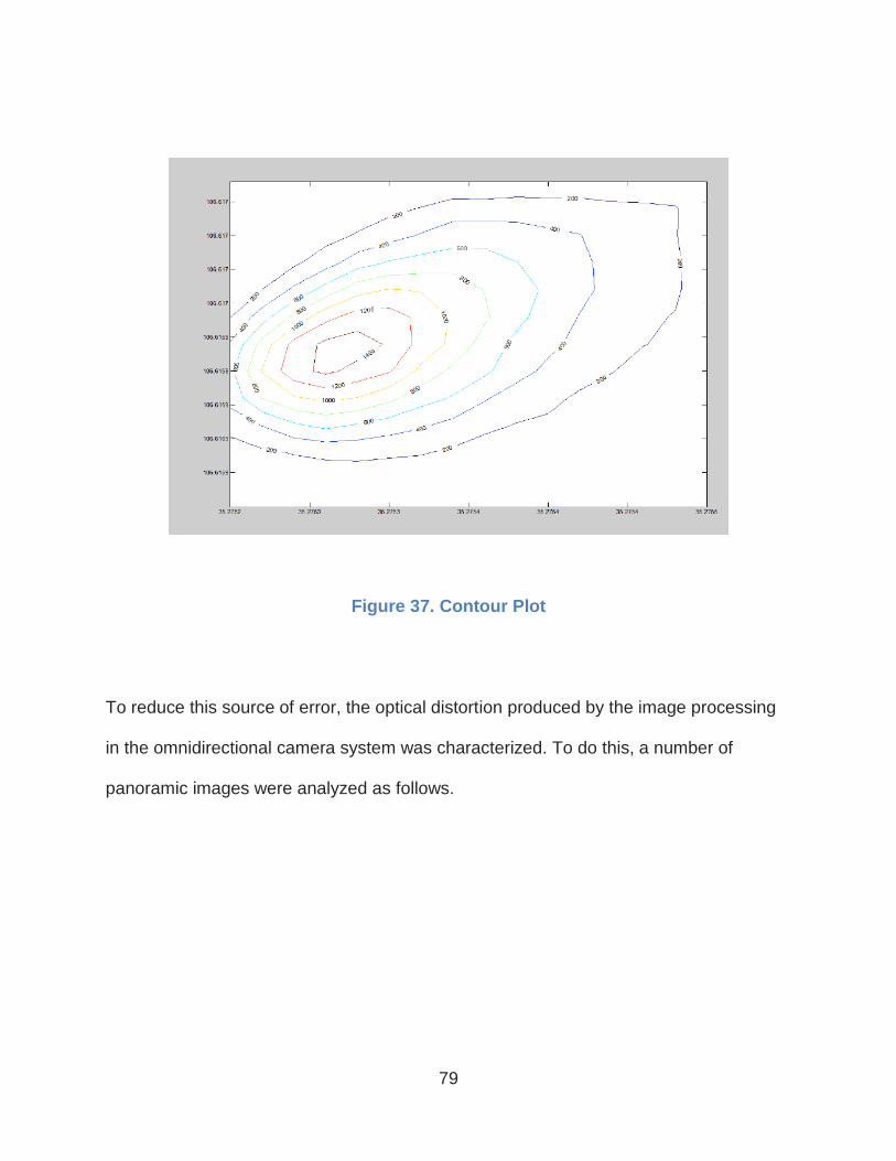
79

Figure 37. Contour Plot

To reduce this source of error, the optical distortion produced by the image processing

in the omnidirectional camera system was characterized. To do this, a number of

panoramic images were analyzed as follows.

80

Figure 38. Error in angle from pixel-based heading estimate

First, in each image, a set of clearly defined features (poles, trees, street signs) were

identified. For each of these features, first the apparent angular position θa was

calculated by assuming that true angular position is proportional to the horizontal pixel

location of the feature. Second, the “true” angular position θt of the feature was

determined manually by maximizing the zoom (12º field of view), centering the feature,

and obtaining the heading of the image from the Street View directly.

The error in angular position, shown in Figure 38, has well-defined characteristics, that

appear to be directly related to the optics and the processing used to obtain the

omnidirectional images. The error can be described by the sinusoidal relationship

81

θe= -4.05 sin(4 θa), where θe = θt - θa. Correcting for optical distortion is, therefore, a

simple matter. For each pair of viewing position, triangulation results in a pole location.

Because an individual pole is usually observed from several camera viewing position

pairs, multiple locations are produced for the same pole that may not coincide perfectly

as a result of the previously discussed positioning errors. This can be used to increase

the accuracy of pole location, owing to the fact that random errors in multiple

observations cancel each other out.

Figure 39. Uncorrected Markers Position

For corrected marker position “position_of_pole” determined in Section 5.2 is

recalculated from formula : Position_of_pole= -4.05*sin(4 * Position_of_pole)

82

Figure 40. Corrected Markers Position

5.4 Clustering

To produce unique locations for each pole, a “gravity clustering” algorithm is adopted.

Like most clustering algorithms, the basic principle is to minimize a potential energy

function that results from the dispersion of points. For this case, the total potential

energy results from an interparticle attractive force with magnitude F = d exp(d/d0),

where d0 is a distance of normalization that sets the distance of maximum attractive

force, which is set to 2m, as shown in the inset in Figure 42.

83

Figure 41. Inter-particle attractive force

“Particles” are interpreted as individual point locations. The particle positions are

adjusted using an Euler explicit calculation until equilibrium (i.e. energy minimization) is

achieved. If points are within certain radius they coalesce to form a single point. An

example of the result of the clustering algorithm is shown in Figure 42, points initially

close to each other coalesce into a single point, but the centroid of one cluster is not

influenced by the position of other clusters.

84

Figure 42. Clustering algorithm: the form of the inter-particle force is shown in the inset. Initial clustered pole locations from multiple triangulations (green squares) coalesce into a single point for each cluster (triangles). The purple line indicates the camera vehicle path, the crosses the location of panorama image collection.

Practical results of the pole location for a path along Corrales Rd., in Corrales, NM, are

shown in Figure 42. Visual inspection reveals that the error in pole location is generally

on the order of 1.5m. This level of accuracy is better than what is possible with a

consumer-grade GPS device, typically on the order of 2.5 m [12].

85

Figure 43. Examples of the location of poles using multiple triangulations from omnidirectional image panoramas. In the majority of cases, the triangulated location is within one meter of the actual pole position.

Figure 44. Clustering Result

Using consumer-grade GPS device badelf, the result for thirty pole position is shown in

figure below (Appendix A.2)

86

Figure 45. Consumer-Grade GPS Result

87

6 Conclusion

6.1 Results of the study

Getting pole location using Google Street view imagery was a success and successful

determination of utility assets was demonstrated in Chapter 5, all these vertical

structures are geo-located using the triangulation and clustering strategy procedure

described, and recorded in a list.

This technology is cost effective and time efficient as compared to current methods of

finding utility assets used by industries which are generally performed by employing at

least two technicians to ride out to transmission and distribution (T & D) lines to

determine reliability issues and position of poles. In their setup usually one drives the

vehicle and other person documents the findings. This method is not just time

consuming but also not economical.

The accuracy of the method discussed in this report is on the order of 1.5m. This level

of accuracy is better than what is possible with consumer-grade GPS device, typically

on the order of 2.5m.

6.2 Future Research

The feasibility of detecting and geographically locating utility assets from public ground-

based imagery databases was demonstrated. A full implementation requires three

88

primary components: a route-planning and imagery collection tool; a geographical

location tool; and a machine-learning-based image analysis tool. By integrating these

components, it will be possible to map and catalog the vast majority of utility distribution

assets that are visible from public roads.

To obtain a fully integrated system, the components described in chapters must be

integrated. For an automated system, image processing algorithm needs to be

optimized to increase detection accuracy, percentage and reduce false detections.

Results obtained from neural image processing need to be integrated to further

minimize user interference and time. Also, this detection process can be done from

multiple locations, to reduce uncertainty in the detection process

In Chapter 4, for large-scale image acquisition, addresses were obtained from real

estate website which does not have a complete database for addresses, because of

that large part of Corrales, NM was not covered. To overcome this, address data from

USPS or any other sources can be purchased in the future and can be integrated with

the code to cover complete area.

Moreover, the application of this technology will be further expanded for the assets

detection on vertical structures and for the height of structures. Poles will be scanned

vertically to find and determine transformer, its type and other assets on the pole.

89

This technology can find applications in planning, maintenance operations, and even

disaster relief. In future, a full characterization of the integrated tool, in terms of location

accuracy, detection accuracy and asset recognition ability will be performed.

90

Appendices

91

Appendix A

Tabular Data

92

Table A.1: Pixels and Angle

Image No. Pixel ( X-coord) Angle

Image 1 34.47 36

Image 1 109.17 106

Image 1 133.47 135

Image 1 262.62 262

Image 1 268.92 266

Image 1 272.52 270

Image 2 24.50 22

Image 2 42.73 46

Image 2 59.60 64

Image 2 74.68 76

Image 2 93.13 90

Image 2 113.83 125

Image 2 221.98 224

Image 3 6.74 159

Image 3 22.04 21

Image 3 27.67 29

Image 3 42.52 43

Image 3 60.29 64

Image 3 88.42 85

Image 3 289.57 287

Image 4 34.46 37

93

Image 4 17.552 20

Image 4 89.66 86

Image 4 124.46 127

Image 4 132.26 136

Image 5 14.05 12

Image 5 22.00 22

Image 5 34.15 37

Image 5 84.40 80

Image 5 98.80 96

Image 5 106.90 105

Image 5 109.30 108

Image 5 121.00 123

Image 5 124.60 128

Image 5 129.40 133

Image6 33.45 27

Image6 37.80 42

Image6 54.00 57

Image6 80.10 76

Image6 92.10 89

Image6 114.60 116

Image6 118.20 121

Image6 123.00 126

Image6 130.20 134

94

Image7 34.48 38

Image7 71.08 67

Image7 105.28 107

Image7 107.98 111

Image7 112.03 115

Image7 119.53 123

Image 8 350.98 348

Image 8 32.38 37

Image 8 44.68 47

Image 8 56.23 55

Image 8 117.28 122

Image 8 186.13 186

Image 8 242.68 240

Table A.2: BadElf Pole Positions

Pole Position GeoLocation

1 35.275482,-106.616959

2 35.275471,-106.616943

3 35.275028,-106.617272

4 35.274879,-106.615753

5 35.274479,-106.614929

95

6 35.273663,-106.613281

7 35.273552,-106.612961

8 35.273022,-106.611855

9 35.272560,-106.610863

10 35.272137,-106.610863

11 35.272137,-106.609840

12 35.271610,-106.609383

13 35.271667,-106.609032

14 35.271191,-106.608002

15 35.270073,-106.606590

16 35.265572,-106.602669

17 35.264690,-106.602402

18 35.264652,-106.602043

19 35.269741,-106.606766

20 35.270813,-106.607185

21 35.273994,-106.613960

22 35.262352,-106.601479

23 35.262585,-106.601486

24 35.262592,-106.601555

25 35.262897,-106.601440

26 35.263008,-106.601433

96

27 35.263466,-106.601501

28 35.263889,-106.601921

29 35.262123,-106.601448

30 35.261646,-106.601387

Table A.3: Camera Locations

1 35.27512 -106.617

2 35.27508 -106.617

3 35.27501 -106.617

4 35.27496 -106.617

5 35.27493 -106.617

6 35.27493 -106.617

7 35.27488 -106.616

8 35.27483 -106.616

9 35.27478 -106.616

10 35.27473 -106.616

11 35.27468 -106.616

12 35.27462 -106.616

13 35.27458 -106.616

14 35.27458 -106.616

15 35.27453 -106.616

97

16 35.27449 -106.615

17 35.27445 -106.615

18 35.27439 -106.615

19 35.27439 -106.615

20 35.2743 -106.615

21 35.27425 -106.615

22 35.27425 -106.615

23 35.27421 -106.615

24 35.27416 -106.615

25 35.27412 -106.615

26 35.27407 -106.615

27 35.27403 -106.614

28 35.27394 -106.614

29 35.27389 -106.614

30 35.27389 -106.614

31 35.27385 -106.614

32 35.2738 -106.614

33 35.27376 -106.614

34 35.2737 -106.614

35 35.27365 -106.614

36 35.27361 -106.614

98

37 35.2736 -106.613

38 35.27352 -106.613

39 35.27348 -106.613

40 35.27338 -106.613

41 35.27338 -106.613

42 35.27334 -106.613

43 35.27329 -106.613

44 35.27327 -106.613

45 35.27322 -106.613

46 35.27317 -106.613

47 35.27312 -106.612

48 0

49 35.27297 -106.612

50 35.27297 -106.612

51 35.27282 -106.612

52 35.27282 -106.612

53 35.27277 -106.612

54 35.27272 -106.612

55 35.27267 -106.611

56 35.27262 -106.611

57 35.27257 -106.611

99

58 35.27251 -106.611

59 35.27246 -106.611

60 35.27238 -106.611

61 0

62 35.27226 -106.611

63 35.2722 -106.611

64 35.27214 -106.611

65 35.27209 -106.61

66 35.27203 -106.61

67 35.27197 -106.61

68 35.27191 -106.61

69 35.27185 -106.61

70 35.27179 -106.61

71 35.27174 -106.61

72 35.27168 -106.61

73 35.2716 -106.61

74 35.27154 -106.61

75 35.27149 -106.609

76 35.27149 -106.609

77 35.27142 -106.609

78 35.27142 -106.609

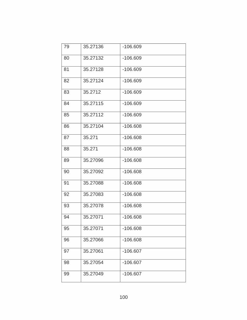
100

79 35.27136 -106.609

80 35.27132 -106.609

81 35.27128 -106.609

82 35.27124 -106.609

83 35.2712 -106.609

84 35.27115 -106.609

85 35.27112 -106.609

86 35.27104 -106.608

87 35.271 -106.608

88 35.271 -106.608

89 35.27096 -106.608

90 35.27092 -106.608

91 35.27088 -106.608

92 35.27083 -106.608

93 35.27078 -106.608

94 35.27071 -106.608

95 35.27071 -106.608

96 35.27066 -106.608

97 35.27061 -106.607

98 35.27054 -106.607

99 35.27049 -106.607

101

100 35.27037 -106.607

101 35.2703 -106.607

102 35.27022 -106.607

103 35.27022 -106.607

104 35.27015 -106.607

105 35.27005 -106.607

106 35.26996 -106.607

107 35.26985 -106.607

108 35.26979 -106.607

109 35.26979 -106.607

110 35.26972 -106.606

111 35.26966 -106.606

112 35.2696 -106.606

113 35.26953 -106.606

114 35.26946 -106.606

115 35.26939 -106.606

116 35.26924 -106.606

117 35.26924 -106.606

118 35.26917 -106.606

119 35.2691 -106.606

120 35.26903 -106.606

102

121 35.26896 -106.606

122 35.26881 -106.606

123 35.26881 -106.606

124 35.26874 -106.606

125 35.26867 -106.605

126 35.2686 -106.605

127 35.26853 -106.605

128 35.26846 -106.605

129 35.26839 -106.605

130 35.26832 -106.605

131 35.26822 -106.605

132 35.26814 -106.605

133 35.268 -106.605

134 35.268 -106.605

135 35.26794 -106.605

136 35.26787 -106.605

137 35.2678 -106.605

138 35.26773 -106.604

139 35.26766 -106.604

140 35.26759 -106.604

141 35.26745 -106.604

103

142 35.26745 -106.604

143 35.26738 -106.604

144 35.26731 -106.604

145 35.26724 -106.604

146 35.2671 -106.604

147 35.26703 -106.604

148 35.26695 -106.604

149 35.26688 -106.604

150 35.26688 -106.604

151 35.26681 -106.604

152 35.26674 -106.603

153 35.26667 -106.603

154 35.26658 -106.603

155 35.2665 -106.603

156 35.26642 -106.603

157 35.26631 -106.603

158 35.26627 -106.603

159 35.26619 -106.603

160 35.26619 -106.603

161 35.26604 -106.603

162 35.26596 -106.603

104

163 35.26596 -106.603

164 35.26587 -106.603

165 35.26578 -106.603

166 0

167 35.26488 -106.602

168 35.26481 -106.602

169 35.26471 -106.602

170 35.26462 -106.602

171 35.26452 -106.602

172 35.26443 -106.602

173 35.26424 -106.602

174 35.26414 -106.602

175 35.2641 -106.602

176 35.26405 -106.602

177 35.26405 -106.602

178 35.2639 -106.602

179 35.2639 -106.602

180 35.26383 -106.602

181 35.2638 -106.602

182 35.26371 -106.602

183 35.26364 -106.602

105

184 35.26358 -106.602

185 35.2635 -106.602

186 35.26343 -106.602

187 35.26339 -106.602

188 35.26328 -106.602

189 0

190 35.26308 -106.601

191 35.26298 -106.601

192 35.26285 -106.601

193 35.26269 -106.601

194 35.26269 -106.601

195 35.26257 -106.601

196 35.26245 -106.601

197 35.26245 -106.601

198 35.26229 -106.601

199 35.26221 -106.601

200 35.26221 -106.601

201 35.26211 -106.601

202 35.26201 -106.601

203 35.26191 -106.601

204 35.2618 -106.601

106

205 35.2617 -106.601

206 35.26159 -106.601

207 35.26146 -106.602

208 35.26141 -106.601

209 35.26135 -106.601

210 35.26135 -106.601

211 35.26125 -106.601

212 35.26117 -106.601

213 35.26106 -106.601

214 35.26106 -106.601

215 35.26097 -106.601

216 35.26088 -106.601

217 35.26068 -106.601

218 35.26059 -106.601

219 35.26059 -106.601

220 35.2605 -106.601

221 35.26041 -106.601

222 0

223 35.2602 -106.602

224 35.26012 -106.602

225 35.26002 -106.602

107

226 35.25984 -106.602

227 35.25981 -106.602

228 35.25981 -106.602

229 35.25962 -106.602

230 35.25962 -106.602

231 35.25953 -106.602

232 35.25944 -106.602

233 35.25935 -106.602

234 35.25925 -106.602

235 35.25916 -106.602

236 35.25906 -106.602

237 35.25895 -106.602

238 35.25883 -106.602

239 35.25872 -106.602

240 35.25861 -106.602

241 35.25852 -106.602

242 35.25844 -106.602

243 35.25834 -106.602

244 35.25819 -106.601

245 35.25819 -106.601

246 35.25814 -106.601

108

247 35.25806 -106.601

248 35.25799 -106.601

249 35.25793 -106.601

250 35.25785 -106.601

251 0

252 35.25773 -106.601

253 35.25761 -106.601

254 35.25754 -106.601

255 35.25754 -106.601

256 35.25747 -106.601

257 35.2574 -106.601

258 35.25731 -106.601

259 35.25725 -106.601

260 35.25717 -106.601

261 35.2571 -106.601

262 35.25703 -106.601

263 35.25695 -106.601

264 35.25686 -106.6

265 35.25676 -106.6

266 0

267 35.25659 -106.6

109

268 35.25659 -106.6

269 35.25651 -106.6

270 35.25633 -106.6

271 35.25625 -106.6

272 35.25625 -106.6

273 35.25617 -106.6

274 35.25608 -106.6

275 35.25596 -106.6

276 0

277 35.25579 -106.6

278 35.2557 -106.6

279 35.25561 -106.6

280 35.25551 -106.6

281 35.25541 -106.6

282 35.25532 -106.6

283 35.25528 -106.599

284 35.25515 -106.599

285 35.25515 -106.599

286 35.25505 -106.599

287 35.25498 -106.599

288 35.2549 -106.599

110

289 35.25482 -106.599

290 35.25472 -106.599

291 35.25463 -106.599

292 35.25455 -106.599

293 35.25438 -106.599

294 35.25438 -106.599

295 35.25429 -106.599

296 35.25421 -106.599

297 35.25412 -106.599

298 35.25401 -106.599

299 35.25393 -106.599

300 35.25385 -106.599

301 35.25376 -106.599

302 35.25359 -106.599

303 35.25359 -106.599

304 35.25351 -106.599

305 35.25342 -106.599

306 35.25332 -106.599

307 35.25323 -106.598

308 35.25314 -106.598

309 35.25305 -106.598

111

310 35.25296 -106.598

311 35.25287 -106.598

312 35.25278 -106.598

313 35.25269 -106.598

314 35.2526 -106.598

315 35.2525 -106.598

316 35.25233 -106.598

317 35.25233 -106.598

318 35.25224 -106.598

319 35.25215 -106.598

320 35.25205 -106.598

321 35.25196 -106.598

322 35.25187 -106.598

323 35.25164 -106.598

324 35.25164 -106.598

325 35.25149 -106.598

326 35.25142 -106.598

327 35.25142 -106.598

328 35.25135 -106.598

329 35.25127 -106.598

330 35.25118 -106.598

112

331 35.25109 -106.598

332 35.25098 -106.598

333 35.25088 -106.598

334 35.25076 -106.598

335 35.25057 -106.598

336 35.25057 -106.598

337 35.25048 -106.598

338 35.25038 -106.598

339 35.25025 -106.598

340 35.25015 -106.598

341 35.25006 -106.598

342 35.24997 -106.598

343 35.24987 -106.598

344 35.24978 -106.598

345 35.2497 -106.598

346 35.24965 -106.598

347 35.2495 -106.598

348 35.2495 -106.598

349 35.2494 -106.598

350 35.24932 -106.598

351 0

113

352 35.24919 -106.598

353 35.2491 -106.598

354 35.24901 -106.598

355 35.24892 -106.598

356 35.24884 -106.598

357 0

358 35.24868 -106.598

359 35.2486 -106.599

360 35.24853 -106.599

361 35.24844 -106.599

362 35.24836 -106.599

363 35.24827 -106.599

364 35.24815 -106.599

365 35.24815 -106.599

366 35.24807 -106.599

367 35.24799 -106.599

368 35.24791 -106.599

369 35.24783 -106.599

370 35.24774 -106.599

371 35.24763 -106.599

372 35.2475 -106.599

114

373 35.24744 -106.599

374 35.24737 -106.599

375 35.24737 -106.599

376 35.24731 -106.599

377 35.24724 -106.6

378 35.24706 -106.6

379 35.24706 -106.6

380 35.24698 -106.6

381 35.24691 -106.6

382 35.24684 -106.6

383 35.24676 -106.6

384 35.24668 -106.6

385 35.2466 -106.6

386 35.24652 -106.6

387 35.24646 -106.6

388 35.24642 -106.6

389 35.24631 -106.6

390 35.24623 -106.6

391 35.24612 -106.601

392 35.24608 -106.601

393 35.246 -106.601

115

394 35.246 -106.601

395 35.24591 -106.601

396 35.2458 -106.601

397 35.2458 -106.601

398 35.24565 -106.601

399 35.24558 -106.601

400 35.24558 -106.601

401 35.24553 -106.601

402 35.24546 -106.601

403 35.24538 -106.601

404 35.24531 -106.601

405 35.24516 -106.601

406 35.24516 -106.601

407 35.24509 -106.601

408 35.24501 -106.602

409 35.24494 -106.602

410 35.24485 -106.602

411 35.24478 -106.602

412 35.24469 -106.602

413 35.24461 -106.602

414 35.24453 -106.602

116

415 35.24446 -106.602

416 35.24427 -106.602

417 35.24427 -106.602

418 35.24415 -106.602

419 35.24409 -106.602

420 35.24397 -106.602

421 35.24397 -106.602

422 35.24388 -106.602

423 35.24379 -106.602

424 35.2437 -106.602

425 35.2436 -106.602

426 35.24351 -106.602

427 35.24343 -106.602

428 35.24335 -106.602

429 35.24326 -106.602

430 35.24317 -106.603

431 35.24308 -106.603

432 35.24299 -106.603

433 35.24289 -106.603

434 35.24279 -106.603

435 35.24268 -106.603

117

436 35.24259 -106.603

437 35.24259 -106.603

438 35.2425 -106.603

439 35.24236 -106.603

440 35.24227 -106.603

441 35.24227 -106.603

442 35.24218 -106.603

443 35.24209 -106.603

444 35.242 -106.603

445 35.24191 -106.603

446 35.24181 -106.603

447 35.24172 -106.603

448 35.24163 -106.603

449 35.24149 -106.603

450 35.24149 -106.603

451 35.2414 -106.603

452 35.24127 -106.603

453 35.24122 -106.603

454 35.24104 -106.603

455 35.24098 -106.603

456 35.24089 -106.603

118

457 35.2408 -106.603

458 35.24066 -106.603

459 35.24057 -106.603

460 35.24057 -106.603

461 35.24043 -106.603

462 35.24039 -106.603

119

Appendix B

Supplementary Data

120

Please refer to supplemental file in LoboVault.

121

References

1. Xcel Energy. (2011). Retrieved from XCELENERGY:

https://www.xcelenergy.com/staticfiles/xe/Regulatory/Transmission/OverheadvsUnderground.pdf.

2. Electricity T&D White Paper. s.l. : NRG Expert, 2013.

3. Center, E. T. (2013). The History of Electrification: The birth of our power grid.

4. Sarfi, R. J., Tao, M. K., Lyon, J. B., & Simmins, J. J. (2012, May). Data quality as it relates to asset

management. In Transmission and Distribution Conference and Exposition (T&D), 2012 IEEE PES (pp. 1-

5). IEEE.

5. Monetizing the Geospatial Information System (GIS): The Value of GIS Data Quality for Electric

Utilities. s.l. : EPRI, 2012.

6. Román, A., & Lensch, H. P. (2006). Automatic Multiperspective Images.Rendering

Techniques, 2(2006), 161-171.

7. Roman, A., Garg, G., & Levoy, M. (2004, October). Interactive design of multi-perspective images for

visualizing urban landscapes. In Proceedings of the conference on Visualization'04 (pp. 537-544). IEEE

Computer Society.

8. Nayar, S. K. (1997, June). Catadioptric omnidirectional camera. In Computer Vision and Pattern

Recognition, 1997. Proceedings., 1997 IEEE Computer Society Conference on (pp. 482-488). IEEE.

9. QuickTime, V. R. (1995, January). An Image-Based Approach to Virtual Environment Navigation,

Shenchang Eric Chen, Apple Computer, Inc. InSiggraph, Computer Graphics Proceedings, Annual

Conference Series (pp. 29-38).

10. Gupta, R., & Hartley, R. (1997). Linear pushbroom cameras. Pattern Analysis and Machine

Intelligence, IEEE Transactions on, 19(9), 963-975.

11. Zomet, A., Feldman, D., Peleg, S., & Weinshall, D. (2003). Mosaicing new views: The crossed-slits

projection. Pattern Analysis and Machine Intelligence, IEEE Transactions on, 25(6), 741-754.

122

12. Anguelov, D., Dulong, C., Filip, D., Frueh, C., Lafon, S., Lyon, R., ... & Weaver, J. (2010). Google

street view: Capturing the world at street level.Computer, (6), 32-38.

13. http://www.google.com/maps/about/behind-the-scenes/streetview/. (n.d.).

14. Farber, D. (2012). Google takes Street View off-road with backpack rig.

15. Google Developers. (n.d.). Retrieved from https://developers.google.com/maps/documentation

16. (n.d.). Retrieved from

https://code.google.com/p/gisgraphy/source/browse/trunk/gisgraphy/src/main/webapp/scripts/v3_epoly.js

?r=67.

17. Stackoverflow. (n.d.). Retrieved from http://stackoverflow.com/questions/430142/what-algorithms-

compute-directions-from-point-a-to-point-b-on-a-map

18. Salmen, J., Houben, S., & Schlipsing, M. (2012, June). Google street view images support the

development of vision-based driver assistance systems. InIntelligent Vehicles Symposium (IV), 2012

IEEE (pp. 891-895). IEEE.

19. Hisham Tariq, A. M. (2015). Geolocation of Utility Assets Using Omnidirectioal Ground-Based

Photographic Imagery. IEEE.