Geol 3050 – GIS for Geologists – Exercise 7

1

Exercise 7 Presenting your Data: Layouts and intro to 3D Displays.

Due: Tuesday, February 11 by start of classGoal: Learn about the Layout View and make a simple 3D Display. Note: Bolstad Chapter 11, page 389‐390.

Datasets: Use the datasets downloaded and adjusted in Exercise 6. You will need:

• cogeology1_projected_Dissolve.shp (Tweto’s 1979 geologic map of Colorado in a LambertConformal projection, centered on ‐105.5 degrees), and dissolved based on our classification – theend product of Exercise 6.

• A Digital Elevation Model (DEM), also projected in a Lambert Conformal Conic projection withcentral meridian ‐105.5 (provided).

Assignment

Every map has a scalebar (or at least latitude longitude information – also called a “graticule”), a north arrow, a title and a legend. Today we will make a nice looking map from your exercise 6 and new data.

Steps I already did for you: A. Downloaded a DEM from the Web. For this, I used the Shuttle Radar Mission Topography data:(http://srtm.csi.cgiar.org/). One could also search the nationalmap.gov site for an appropriate

GIS‐ready DEM. First I had to mosaic the data.

B. Projected the WGS84 data to the 1927 NAD to match the Tweto map.C. Clipped the DEM to the boundaries of Colorado by opening the Toolbox and going to DataManagement Tools > Raster > Raster Processing > Clip.

Steps you need to do today: A. Make a hillshade of your DEM for a nice base image.B. Make a 3D drape of your map in ArcScene.

C. Make a spiffy Layout.

Part A. Make a Hillshade from your DEM

Workflow Part A

1. Open ArcMap, preferably your own map document from Exercise 6. If you don’t have that saved,quickly rebuild your project (see exercise 6), with the cogeology1_Project_Dissolve layer added andcolored according the previously given color scheme.

2. Download the CO_DEM.zip from our website, unzip, and add the layer to your map document.Check the projection! Make sure it is Lambert Conformal Conic!

3. Check for overlap: Does the DEM match the boundaries of your Dissolved CO Geology Map?

Geol 3050 – GIS for Geologists – Exercise 7

2

4. To improve our visual effect, we can apply an algorithm to our DEM to artificially illuminate ourtopography. This is also called a “Hillshade” effect.

5. Make sure the Arc Extensions are turned on by going to Customize > Extensions and thencheckmark the boxes (need 3‐D Analyst and Spatial Analyst for this exercise).

6. Go to Arc Toolbox, and follow the path Spatial Analyst Tools > Surface > Hillshade

7. Open the tool, and enter the following parameters:

8. Save your file on your flash drive.

9. Your new dataset “CO_hs” will be automatically added to your map.

Part B. Make a 3D drape of the geology in ArcScene

Workflow Part B

10. Still in the “data view” of ArcMap, zoom to the full extent of the geologic map (do this by clicking onthe little globe on your Tools toolbar).

11. Make sure the order of the layers is:

• co_geol_Project_Dissolve.shp (Projected and Dissolved map from Ex. 6)o Also with Transparency of 50%

• Colorado hillshade clipped to match the geology.

• Turn the other Layers off!!

Your map should look like this, with no edges showing from beneath the geology:

Geol 3050 – GIS for Geologists – Exercise 7

12. Go to File > Export Map

13. Fill out the dialog as follows:

Make sure to check the Write World File. Before you hit save, click on Format tab and check the Write GeoTIFF

Tags box. Now you can hit save. 3

4

You can check this out by moving the “Scene” around:

Geol 3050 – GIS for Geologists – Exercise 7

Why this step? When you drape shapefiles directly in 3D, you often get a weird looking, “curtain”‐ like effect. This is because only the vertex points of every polygon or line are plotted directly on the DEM. The lines or surfaces in between the polygons are extrapolated for their elevation in between these points, as straight lines. This will most of the time look unacceptable.

Therefore, we are using a raster format, an image, to drape. So, we are exporting our nice look from the data view to image format and saving the coordinates (via the World File!) We can then directly use this file in ArcScene.

14. Open ArcScene (part of ArcGIS). Select a blank scene.

15. Add the following layers to ArcSence in this order(!) ("+" button or copy/paste from ArcMap)

• co_geol_Project_Dissolve.shp• The Digital Elevation Model (topography) –clipped (CO_DEM)

• The newly exported CO_geol_drape.tif fileo You may build pyramids on both.

16. Notice that all layers show up, but do not have any elevation, and that they plot on top of eachother.

17.

Use your left‐ right and mouse‐wheel button, similar to Google Earth!

18. Go to the Properties of the CO_geol_drape.png layer (the one we just exported from ArcMap)

19. Notice that the Properties are slightly different than in ArcMap:

We are now going to set the elevation for the geologic map:

20. Go to the Base Heights TAB.

21. Set the heights for this surface to your Colorado DEM clip and click OK

Geol 3050 – GIS for Geologists – Exercise 7

5

This will use the elevation values of the Colorado DEM to drape the geology image:

22. Look back at your “scene”. Can you see the result?

Probably just barely! But it is there…

23. To enhance the effect, set the Vertical Exaggeration via the Scene Properties:

• Right click on Scene Layers, and scroll down to Scene Properties• Set the Vertical Exaggeration to 10

24. Turn off all layers (also the DEM) except for CO_geol_drape.tif as only one.

25. Play around with your view.

If you like you can take the “Co_geol_Project_Dissolve.shp layer adjust the base heights the same way as you adjusted them for the draped image (so set them to the CO_DEM). Can you see the curtains (I set my transparency to 50% upder Properties>Display)

Geol 3050 – GIS for Geologists – Exercise 7

6

26. Again, turn off all layers (also the DEM) except for CO_geol_drape.tif

27. Keep track of where North is as you will need to know that in the next step!

28. When you find a nice view perspective, stop there and go to File > Export > 2D

29. Export your View as a tiff image, (200 dpi), that we will import back into ArcMap for our Layout!

Part C. Integrating it all in a Layout

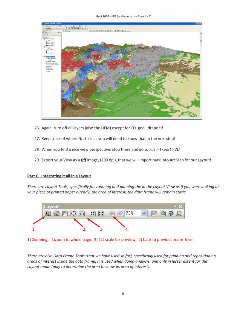
There are Layout Tools, specifically for zooming and panning the in the Layout View as if you were looking at your piece of printed paper already, the area of interest, the data frame will remain static.

1. 2. 3. 4.

1) Zooming, 2)zoom to whole page, 3) 1:1 scale for preview, 4) back to previous zoom level

There are also Data Frame Tools (that we have used so far), specifically used for panning and repositioning areas of interest inside the data frame. It is used when doing analysis, and only in lesser extent for the Layout mode (only to determine the area to show as area of interest).

Geol 3050 – GIS for Geologists – Exercise 7

7

Make sure you play with these and know the difference!

Setting up the Page

30. Go to View > Layout View

31. Go to File > Page and Print Setup and choose either Portrait or Landscape. Also check the checkboxfor “Scale map elements proportionally to changes in page size.” And click OK.

32. Adjust the size of your dataframe by pulling the little squares on its edges, and make sure it fits thepage nicely and that there is still room for a legend and a title, a picture (your ArcScene Export) andan Index Map.

33. Go to Insert > Insert Title, and type Geology of Colorado, or Age Distribution of Rocks in Colorado, oranother useful title for this map.

Making an Index Map

34. Go to Insert > Data Frame

35. For this new dataframe add the Worldcountry.shp layer (via the PLUS button) we used in Exercise 5.(You can re‐download and extract this file from: geode.colorado.edu\~geol3050).

36. Give the countries some appropriate symbology (even no fill would do with just a black outline).Zoom in to the US/North America (via the data frame zooming tools!).

37. Go to the “New Data Frame” > Properties

38. Go to Extent Indicators TAB:

• Set the other Data Frame (i.e. Layers) to show up as an extent rectangle inside the Data.You can set the color (optional: red?) and line thickness (maybe 2) via the Frame Button:

Geol 3050 – GIS for Geologists – Exercise 7

8

Make sure you can see in your map what happened! This will give the outline of the Layers ‐Data Frame, even if you zoom in or out in the geologic map! The Data Frames are now dynamically linked.

Making a Legend

39. Go to Insert > Insert Legend, add a legend for the cogeology1 layer. Make sure no other layers showup in the legend, as a legend for a hillshade is not appropriate in this case.

40. You can make the legend prettier by adjusting the cogeology_dissolve layer name into “Ages ofColorado Rocks” via the Table of Contents (click lightly on the name two times to rename).

41. You can also add some more text to the legend under Layer Properties> Symbol in the Label field

42. Uncheck the “All other Values button, as it will make the legend prettier too. An example:

Geol 3050 – GIS for Geologists – Exercise 7

9

Age Of Colorado Rocks

Cenozoic Igneous

Cenozoic Sedimentary

Cenozoic Unconsolidated

Mesozoic

Paleozoic

Precambrian

Water

More touching up:

43. Insert your 3D Map via Insert > Picture

44. Add a North Arrow (via the Insert Menu) for the geologic map.

45. Hand draw a north arrow for your 3D map, in the correct north direction. Or Insert a north arrowand rotate it to show north correctly.

46. Add a graticule (Data Frame Properties > Grids) of 1 degree intervals for the geologic map (as wedid in exercise 5).

47. Insert a scalebar and change the properties of the default:

• Change the way it displays axes and tics by going too Scale and units > adjust width to a value that makes sense NOT 2.345 km intervals, or

something like that.

o Adjust the division value (Use the “Adjust Width” option).o Adjust the units to be either meters or miles!

48. Add a text box (Insert > Text) with your name and another one with projection information(remember all the settings? If you forgot, you can peek under “Data Frame Properties”, CoordinateSystem)! You only need to mention the projected coordinate system, central meridian and yourdatum!

Make the font of these small.

54. Experiment with adding neatlines (new rectangle‐ tool), i.e. little boxes around the legend and text.

55. Make sure all your map items are distributed nicely over the piece of paper and empty white space isminimized. It must be nice to look at.

Think about the 5 D’s of map making…are all ingredients there and appropriate? Design, Density, Description, Distance, Direction

Geol 3050 – GIS for Geologists – Exercise 7

10

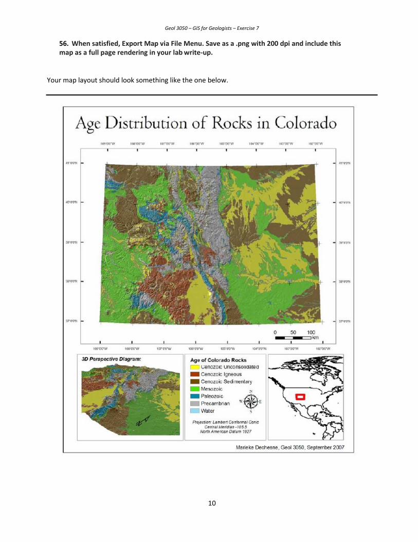
56. When satisfied, Export Map via File Menu. Save as a .png with 200 dpi and include thismap as a full page rendering in your lab write-up.

Your map layout should look something like the one below.

11

From now on, when you are asked to turn in a complete map layout rather than a screenshot, it should be constructed similarly to what you now have (though the number of actual maps and insets will differ). The following items should always be included along with any other specific information: title, name, a grid/graticule, a legend that includes all symbolized data, a north arrow, scale bar, and your projection/meridian/datum.

Part D.

Now, let’s put our map on Google Earth so you can learn how to portray any GIS layer in this powerful software!

1. Open ArcMap if you don’t already have it open and make sure the co_geol_Project_Dissolve.shp layeris available. (you can just reopen the .mxd from Ex. 6 if you wish).

2. Open Arc Toolbox and go to Conversion Tools > To KML > Layer to KML3. Once the Map to KML dialogue box is open, fill out the parameters as follows:

• Layer: use your Exercise 6 dissolved map of Colorado

• Ouptut File: **name this something you will remember

• Map Output Scale: 50000

• Clamped features to ground box is checked.4. Now, open Google Earth.5. Right Click on My Places (which is located in the Places drop down menu on the left hand side of the

screen).6. From there go to Add > Network Link.7. Name the file as you wish, then under Link use the Browse button to go to your class folder and select

your recently made .kml file. Click Open, then OK. Find your file listed under Places and double click on it.Check out what happens!

8. Under Tools>Options> change the elevation exaggeration to the max (3).9. Expand the “Borders and Labels” in the table of contents. Uncheck the “Borders” box but turn on

(check) the “Places” box. Also turn on “Roads” and “Terrain” if they aren’t already checked. All otherlayers should be off.

Part D Questions to Answer:

D.1) Given our definition of a Geographic Information System (a computer‐based system to aid in thecollection, maintenance, storage, analysis, output, and distribution of spatial data and information), isGoogle Earth a true GIS? Why or why not?

D.2) What are the different advantages of ArcGIS and Google Earth?

Now fly around in Google Earth so you have a perspective view looking west with Boulder in the foreground. It should look something like the view on the next page. Then answer these questions.

D.3) What are the rock units under the city of Boulder? (Hint: you can click on the colors to identify)

D.4) What is the age of the rocks that make up Boulder Canyon?

12

D.5) Capture a screenshot of your perspective view akin to the one on the next page and include this in your labreport.

Note that ArcGIS also has a similar functionality to Google Earth. From the Programs folder, open upArcGlobe. Try to add your CO geologic map. Does it work?

(Hint: if the colors don’t match your rock type/age classification there’s an easy fix. In ArcMap, right‐click onyour co_geol_Project_Dissolve layer and click Save as Layer File. After you’ve made that layer file, go back toArcGlobe. Then Right click on your co_geol_Project_Dissolve layer, go to Properties> Symbology. Then click“Import” and navigate to your layer file.)This will apply the color classification from the map layer in ArcMap to the one in ArcGlobe. Make ascreenshot and caption and include it with the one above in your lab report.

Your lab report should include all of the following: Your complete one-page map layout. Your answers to questions D.1 – D.5 including two screenshots on a separate page. Turn in both parts by the start of class next week.