Acta Geodyn. Geomater., Vol. 13, No. 1 (181), 19–26, 2016

DOI: 10.13168/AGG.2015.0041

journal homepage: http://www.irsm.cas.cz/acta

ORIGINAL PAPER

GEOID DETERMINATION FOR THE AREA OF POLAND BY THE LEAST SQUARES MODIFICATION OF STOKES' FORMULA

Joanna KUCZYNSKA-SIEHIEN*, Adam LYSZKOWICZ and Monika BIRYLO

University of Warmia and Mazury in Olsztyn, Oczapowskiego 1,10-719 Olsztyn, Poland

*Corresponding author‘s e-mail: joanna.kuczynska@uwm.edu.pl

ABSTRACT

Previous geoid/quasigeoid models calculated for the area of Poland were based on the traditional“remove-compute-restore” procedure. One of the modifications of this method is the leastsquares modification of Stokes’ formula with additive corrections method (LSMSA), which wasdeveloped at the Royal Institute of Technology (KTH) in Stockholm in Sweden. The modifiedStokes integral combines the regional terrestrial gravity data with a global geopotential model(GGM) giving the approximate geoid heights. To obtain the gravimetric geoid, four additivecorrections, topographic, downward continuation, atmospheric and ellipsoidal, are calculated andapplied. This paper presents the results of computation of a new gravimetric geoid model for Polandusing the KTH method. In computations terrestrial gravity anomalies derived from nine differentgravimetric data sets, global geopotential model EGM2008 and global elevation data SRTMv. 4.1 were used. The determined gravimetric geoid model was evaluated with GPS/levellingpoints of the Polish ASG-EUPOS network. After fitting the geoid model to the GPS/levellingdata using a 7-parameter model, the standard deviation of differences was estimated to 2 cm.

ARTICLE INFO

Article history:

Received 10 February 2015 Accepted 13 July 2015 Available online17 September 2015

Keywords: KTH method of geoid modelling Rgional geoid determination Stokes integral

where the term NGM reflects the contribution of thegeopotential model coefficients, while N∆g representsthe contribution of the Faye’a anomalies (∆g) afterremoving the effects of the geopotential model. Theterm NH is called the indirect effect on the geoid, andaccounts for the change of equipotential surface afterthe terrain reduction is applied to ∆g. The term N∆g

can be calculated using the Fast Fourier Transform orthe least squares collocation method (Łyszkowicz,2012; Kryński, 2007). Accuracy of the last quasi-geoid model computed from gravimetric data andgeopotential model EGM08 by the collocation methodafter fitting to the vertical reference height system inPoland is accurate to ± 1.4cm (Łyszkowicz, 2010).

But at the same time, there are no geoid modelsfor Poland computed using the LSMSA method (leastsquares modification of Stokes’ formula with additivecorrections). In order to determine the next geoidmodel for Poland, this method was used in this paper.The method was developed at the Royal Institute ofTechnology (KTH) in Stockholm and is also known asthe KTH method. This method was successfullyapplied for a gravimetric geoid determination inseveral countries. The results of the regional geoidmodelling using the KTH method were given amongothers in (Ågren, 2004; Ellmann, 2004; Kiamehr,2006; Abdalla 2009; Ulotu, 2009; Ågren et al., 2009;Daras et al., 2010).

The KTH method utilizes the least squaresmodification of the Stokes integral for the biased,unbiased, and optimum stochastic solutions. Theprinciple of this modification is to match errors within

1. INTRODUCTION

Geoid model determination is a crucial challengein the development of the Earth sciences. Knowledgeof the precise geoid model contributes to the study ofthe Earth’s interior, long-term geophysical processesand is used in oceanography. An accurate regionalgeoid model, in particular, enables the user in manycases to replace the traditional height determinationtechniques by faster and more cost-effective GPS-levelling.

In Poland, over the years, a number ofgeoid/quasigeoid models were calculated based ondifferent methods. The first regional astro-gravimetricgeoid model for Poland was developed in 1961(Bokun, 1961), whereas the last astro-gravimetricgeoid model was computed in 2005 on the basis ofcorrected astro-geodetic and astro-gravimetricdeflections of the vertical (Rogowski et al., 2005).The first gravimetric geoid model for the region ofCentral Europe, including Poland, was computed by(Tanni, 1949). The first gravimetric geoid model forPoland (geoid92) was calculated at the Department ofPlanetary Geodesy in Warsaw in 1993. To computethis geoid the least squares collocation combined withthe integral method was used (Łyszkowicz, 1993). Itis estimated that the accuracy of this geoid model is ofthe order of ± 26 cm (Łyszkowicz, 1993).

Further gravimetric quasigeoid models werecalculated using technique "remove-compute-restore"according to the formula

GM g HN N N NΔ= + + (1)

Cite this article as: Kuczynska-Siehien J, Lyszkowicz A, Birylo M: Geoid determination for the area of Poland by the least squaresmodification of Stokes´ formula, Acta Geodyn. Geomater. 13 (1) (2016) 19–26. DOI: 10.13168/AGG.2015.0041

J. Kuczynska-Siehien et al.

20

where 0N is the approximate geoid height, TopocombNδ is

the combined topographic correction, which includesthe sum of the direct and indirect topographicaleffects on the geoid heights; DWCNδ is the downward

continuation correction, acombNδ is the combined

atmospheric correction, which includes the sum of thedirect and indirect atmospherical effects, and eNδ is

the ellipsoidal correction for the sphericalapproximation of the geoid in Stokes’ formula toellipsoidal reference surface.

The approximate geoid height 0N is calculatedbasing on modified Bruns-Stokes’ formula (Sjöberg,2003c):

( )0

0

22

MGGM

L n nn

cN S g d c b g

σ

ψ Δ σ Δπ =

= + (3)

where the first term of the equation (3) containsmodified Stokes’ function ( )LS ψ and is computed

using Faye’a anomalies gΔ with the spherical cap

0σ , parameter c = R/2γ0, where R is the Earth’s mean

radius, and γ0 is the mean normal gravity. The secondterm represents the Global Geopotential Model(GGM) contribution to the approximate geoid heightand GGM

ngΔ is the Laplace spherical harmonics of the

gravity anomaly calculated from the GGM of degreen, M is the maximum degree of GGM, bn is the least-squares modification parameters.

Precise geoid height is obtained by applying fouradditive corrections. The combined topographic effect

TopocombNδ is the sum of the direct and indirect effects,

and is calculated using formula (Sjöberg, 2000):

2 22 2

3Topocomb dir dir

i

GpN N N H H

R

πδ δγ

= + = − + (4)

where ρ is the mean topographic mass density, G isthe gravitational constant, γι is the normal gravity andH is the orthometric height.

terrestrial gravity data and the global geopotentialmodel (GGM) omission and commission errors bymeans of the least squares. In the method the satellite-only GGM are using what is discussed, for example,at work (Vaníček and Sjöberg, 1991). The maindifference between the KTH method and otherapproaches to the gravimetric geoid determinationcomes from a different treatment of the gravitycorrections. In conventional Stokesian approaches, theobserved gravity anomalies are first corrected for thetopographic and atmospheric gravitational effects andthen reduced to the geoid surface. In the KTH method,the Stokes integration is applied directly to the gravityanomaly data. The complete contribution of the directand secondary indirect effects of topography andatmosphere on the gravity anomalies andconsequently the primary indirect effects oftopography and atmosphere on the geoid heights aretreated as the combined topographic and atmosphericcorrections applied to the approximate geoid heights(Sjöberg, 2003b). The contribution of the downwardcontinuation of the gravity anomalies from the Earth’ssurface onto the geoid surface is added to theapproximate geoid heights as the downwardcontinuation correction. The geoid heights are alsocorrected due to the ellipsoidal approximation of theEarth’s shape.

The KTH method is briefly discussed in Section2. Description of the utilized data is given in Section3. The geoid computation results are shown in Section4. Section 5 gives the results of the computed geoidmodel validation using GPS/levelling data.Conclusions could be found in Section 6.

2. LSMSA METHOD

The computational procedure for estimation of

the geoid height N

using KTH method can besummarized by the following formula (Sjöberg,2003b):

0 Topo acomb DWC comb eN N N N N Nδ δ δ δ= + + + +

(2)

Downward continuation effect in the KTH method is computed applying following formulas:

( ) ( ) ( ) ( ) ( )1 1 2L ,Far LDWC DWC DWC DWCN P N P N P N Pδ δ δ δ= + + (5)

( ) ( ) ( ) 01 1

32

pDWC p p

pp

g P gN P H H

r r

ςΔ Δδγ γ

∂= + − ∂ (6)

( ) ( ) ( )2

1

2

1

nM

L ,Far M GGMDWC n n n

n p

RN P c s Q g P

rδ Δ

+

∗

=

= + −

(7)

( ) ( ) ( )0

2

2LDWC L p Q Q

p

c gN P S H H d

rσ

Δδ ψ σπ

∂= − ∂ (8)

where P is the computation point, 0pς is an approximate value of the height anomaly and Q is the running point

in Stokes’ integral, rp = R + HP, and n ns s∗ = , if 2 n M≤ ≤ , otherwise 0ns∗ = , ns is the modification parameter,

see (Ågren, 2004).

GEOID DETERMINATION FOR THE AREA OF POLAND BY THE LEAST SQUARES … .

21

The combined atmospheric effect acombNδ can be approximated using the equation:

0 0

2 1

2 22 2 2

1 1 2 1

Ma L Lcomb n n n n n

n n M

R R nN s Q H Q H

n n n

π ρ π ρδγ γ

∞

= = +

+ = − − − − − − − + (9)

where ρ0 is the atmospheric density at sea level, and Hn is the Laplace harmonic of degree n for the topographicheight.

The ellipsoidal correction eNδ to the modified Stokes’ formula takes the following form:

( )2

2

2 1L GGM

e n n n e nn

R a R aN s Q g g

n R Rδ Δ δ

γ

∞∗

=

− = − − + − (10)

where formula for ( )e ngδ calculation with necessary coefficient explanation is given by (Sjöberg, 2004).

All these gravimetric data were referred to thenormal field defined by GRS80 ellipsoid and IGSN71gravity reference level.

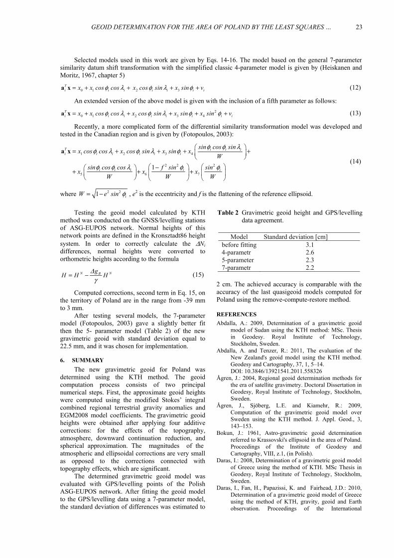
In order to determine the geoid using the KTHmethod, free-air gravity anomalies (Kryński, 2007)were interpolated by the least squares predictionmethod on 1.5' x 3.0' grid nodes for the area 47o <ϕ<57o and 11o <λ <27o (Fig. 1). The GRAVSOFTprogram geogrid.for (Forsberg and Tscherning, 2008)was applied for this task. The geogrid.for programuses covariance function parameters with variance C0

and correlation length ξ (Fig. 2). To determine theseparameters from gravity data, empcov.for programwas used. The obtained results are equal to45600 (μms-2)2 for variance and 35.5’ (65.8 km) forcorrelation length.

As a result of interpolation, a set of 128,721gravity anomalies were obtained. This set of gravityanomalies is characterized by a mean value 62.4 μms-2

(6.24 mGal) and a standard deviation 231.6 μms-2

(23.16 mGal). In a new geoid model calculations global

geopotential model EGM2008 was used. The resultsof evaluation tests have revealed that the EGM08model is very accurate over all existing geopotentialmodels for the area of Poland (Łyszkowicz, 2009).EGM2008 is a spherical harmonic model of theEarth's gravitational potential, developed by a leastsquares combination of the ITG-GRACE03Sgravitational model and its associated error covariancematrix, with the gravitational information obtainedfrom a global set of area-mean free-air gravityanomalies defined on a 5 arc-minute equiangular grid(Pavlis et al., 2012).

SRTM data v. 4.1 was chosen as a digitalelevation model (DEM) and used in the processing.The SRTM DEM has a resolution of 90 m at theequator, and are provided by the CGIAR-CSIGeoPortal for the entire world (http://srtm.csi.cgiar.org).The data are derived from the USGS/NASA SRTMdata. Areas with regions of no data in the originalSRTM data have been filled using interpolationmethods described by (Reuter et al., 2007).

More details about the theoretical basis of themethod, including computation of signal and noisedegree variances, are presented e.g. by (Sjöberg, 1984,1991, 2003a, 2003b, 2003c; Ellman, 2004; Daras,2008; Ågren et al., 2009; Abdalla and Tenzer, 2011). 3. DATA

Gravimetric data used in this work consists ofnine sets of gravity anomalies (Fig. 1) obtained fromvarious sources and collected in the years from 1990to 1995 at the Department of Planetary Geodesy atSpace Research Centre in Warsaw (Łyszkowicz,1994). The data from the Czech Republic, Slovakia,Hungary, Romania and Western Ukraine wereprobably developed in a consistent manner that isbased on the Bouguer anomaly map, which assumesthe density of the Earth's crust is equal to 2.67 g/cm3.The mean gravity anomalies were probably created asthe average values in the 5' x 7.5' areas. The numberof measurements in the block is not known. For thesedata information about the accuracy is also unknown.In contrast, gravity anomaly collections from the areaof Poland are well-documented.

Land gravimetric measurements on Polishterritory were made over the period 1957 - 1979 usingAskania, Sharpe, Scintrex, Sodin and Wordengravimeters. In total, approximately 1,000,000 pointswere measured with mean error of free-air gravityanomaly no greater than ± 0.5 μms-2 (Królikowski,1994). The original anomalies have been converted toanomalies related to normal field of GRS80 ellipsoidand IGSN71 gravity reference level. Subsequently,these anomalies were interpolated on 1' x 1' grid nodes(Kryński, 2007, p. 135) and used in our geoidcomputation.

Sea gravimetric measurements on the southernpart of Baltic Sea were carried out in 1978 -1980. Thetotal number of measured points is 8,423. The meanerror of computed free-air gravity anomalies isestimated as ± 5.7 μms-2. On the basis of themeasured point anomalies, 14,981 mean anomalies on1' x 1' grid nodes were interpolated. The accuracy ofthe mean marine anomaly is estimated to be ± 4 μms-2

(0.4 mGal) (Łyszkowicz, 1994).

J. Kuczynska-Siehien et al.

22

Table 2 Gravimetric geoid height and GPS/levellingdata agreement.

Model Standard deviation [cm] before fitting 3.1 4-parametr 2.6 5-parameter 2.3 7-parametr 2.2

Table 1 Statistics of results (in m).

Minimum Maximum Mean Standard Deviation

Approximate geoid height 0N 22.221 47.932 35.389 6.654 Combined topographic correction -5.325 0.006 -0.082 0.181 Downward continuation correction -0.027 0.216 0.003 0.010 Atmospheric correction -0.002 0.002 0.001 0.001 Ellipsoidal correction 0.000 0.003 0.001 0.000

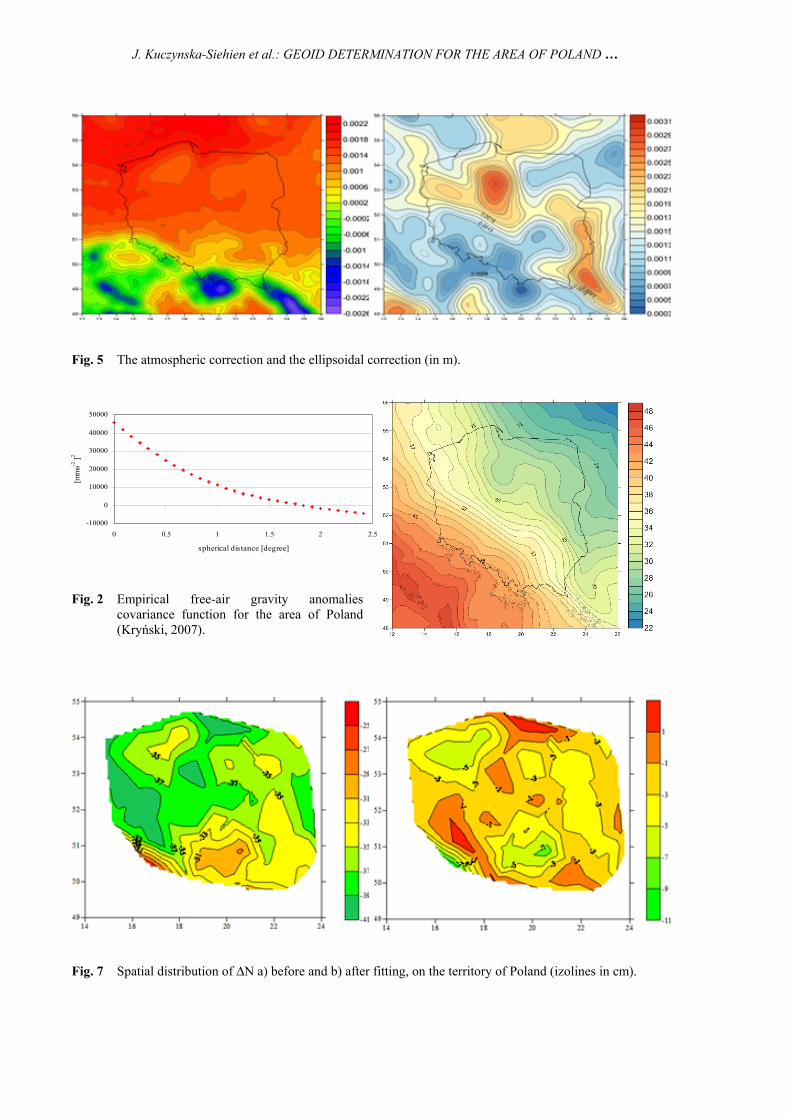
The calculated combined atmospheric correctionand ellipsoidal correction are illustrated respectivelyin Figure 5. Combined atmospheric correction iscomputed using Eq. 9, whereas ellipsoidal correctionusing Eq. 10. The aforementioned additive correctionsdepend on the modification method, cap size andmaximum degree of the GGM being used. Themaximum degree of the GGM is still M = 360. Boththe atmospheric and ellipsoidal corrections are of theorder of millimeters and are almost not significant.

The last step in the geoid height N

computationusing LSMSA method is adding up all the partscalculated in the previous steps according to Eq. 2.Results are illustrated in Figure 6. Evaluation of thecomputed gravimetric geoid model is described in thenext section.

The full statistics of the above constituencies ofEq. 2 is given in Table 1.

5. EVALUATION OF THE COMPUTED

GRAVIMETRIC GEOID MODEL

Currently, evaluation of the accuracy ofcalculated geoid models is realized by theircomparison with the geoid spacing computed fromindependent data, that is from ellipsoidal heightsobtained by GNSS measurements and orthometricheights H from geometric levelling and gravity data.

In practice, due to the occurrence of variousrandom and systematic errors in h, H and N, theknown relationship for each i point

0i i ih H N− − = (11)

is not fulfilled, and we get

i i i ih H N ε− − = (12)

The elimination of systematic factors iε is

necessary in order to properly assess the calculatedgeoid model. This task can be accomplished by leastsquares method using the extended observationequation

Ti i ivε= +a x (13)

in which additional parameters (nuisance) x and thevector of coefficients ia dependent on the spatial

point position were introduced. Examples ofparametric models, which were used to describesystematic factors in a mixed set of geometric,orthometric heights and geoid-ellipsoid separations,can be found in the paper (Fotopoulos, 2003).

The obtained geoid model was evaluated usingthe ASG-EUPOS network. It is a network ofpermanent GNSS stations established for surveyingpractice and has been operating fully since 2008. Thenetwork is based on 98 reference stations situated inPoland and 22 foreign stations. The complete set ofcoordinates of the domestic reference stations of theASG-EUPOS system used in this paper are in ETRF-2000 coordinate system and was downloaded from thewebsite www.asgeupos.pl. The ellipsoidal heights ofthe network points were determined with an accuracyof 1 cm. The normal heights of these points weredetermined in the Kronsztadt86 datum by connectingthem to the national precise levelling network.

4. GEOID COMPUTATION AND RESULTS

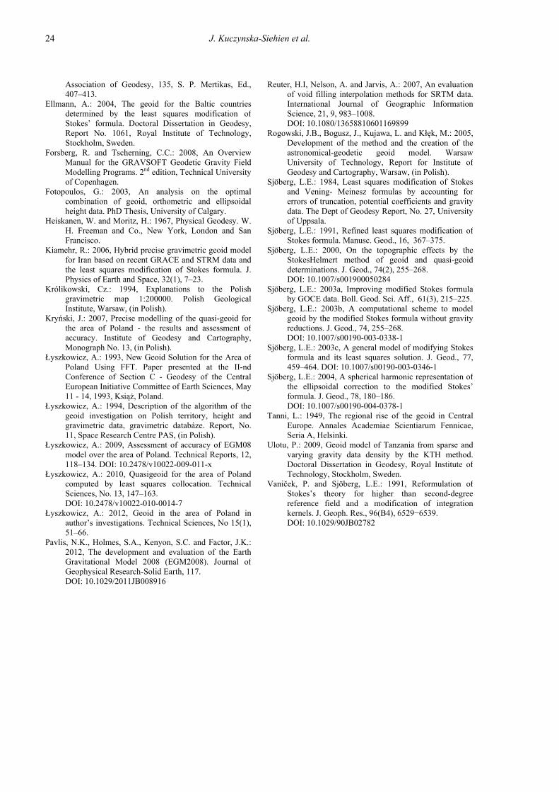
Based on Eq. 2, approximate geoid height 0Nwas calculated in 1.5' x 3.0' grid. The South-Westcorner of the target area grid has ϕ = 48◦ and λ = 12◦,while the North-East has ϕ = 56◦ and λ = 26◦. Incomputation EGM2008 model was used up to degree360. The part of the determined geoid from terrestrialgravity data is shown on the left side of Figure 3,whereas the part of the determined geoid from GGMon the right side. By adding the two foregoing gridfiles we got the approximate geoid height which wasready for applying correction terms.

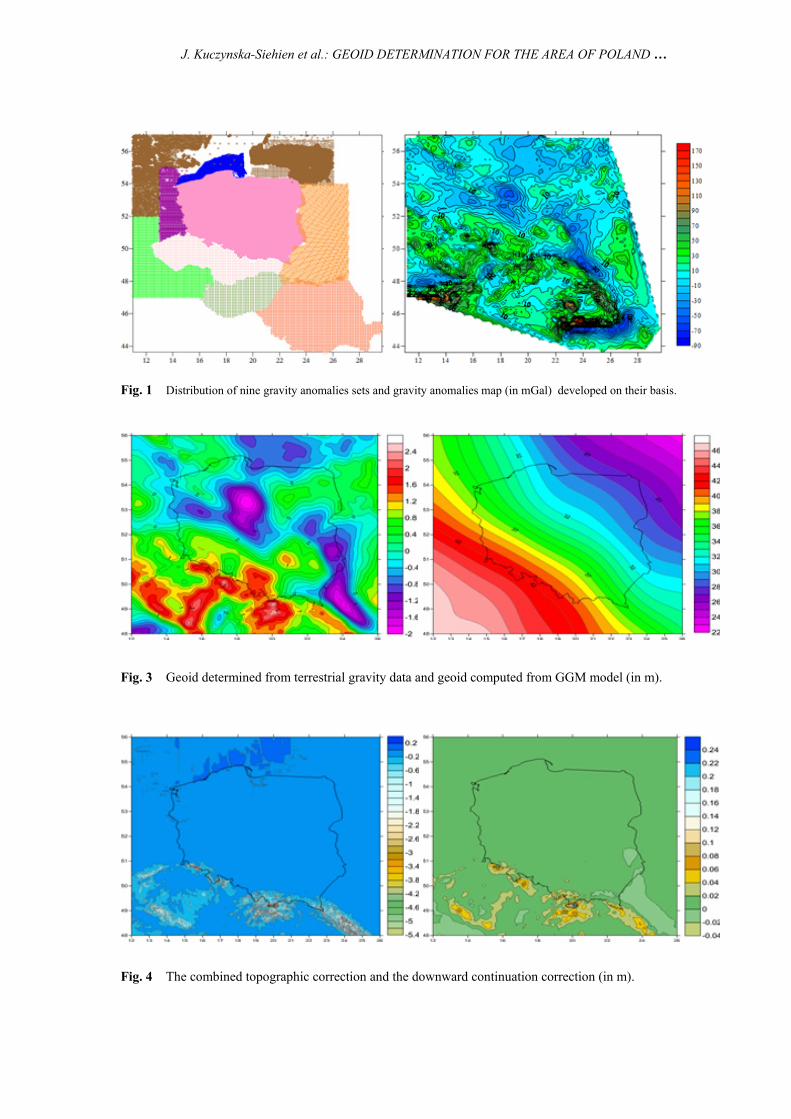
The KTH technique for geoid adds the direct andindirect effects on the geoid heights giving thecombined topographic correction, which was obtainedusing Eq. 4. Moreover, topographic effects is alsoconnected with a downward continuation correction,which is used to reduce gravity data located at surfaceof the Earth to sea level (approximated by a sphere) tobe consistent with Stokes formula. The downwardcontinuation correction was computed according toEq. 5. Topographic heights, necessary to computeboth corrections were interpolated from SRTM data v.4.1 (see Sect. 3). In the downward continuationcorrection calculations EGM2008 with M = 360 wasinvolved. The magnitude of the combined topographiccorrection is illustrated on the left side of Figure 4,whereas downward continuation correction on theright side. It is clear that the topographic effects arelarge in the mountainous areas in the Southern part ofPoland. In the lowlands, the downward continuationcorrections are at the 1-cm level. The combinedtopographic effect is very significant, reaching a fewmeters for the highest part of the mountain. However,part of this effect is counteracted by the downwardcontinuation effect.

GEOID DETERMINATION FOR THE AREA OF POLAND BY THE LEAST SQUARES … .

23

Selected models used in this work are given by Eqs. 14-16. The model based on the general 7-parametersimilarity datum shift transformation with the simplified classic 4-parameter model is given by (Heiskanen andMoritz, 1967, chapter 5)

0 1 2 3Ti i i i i i ix x cos cos x cos sin x sin vφ λ φ λ φ= + + + +a x (12)

An extended version of the above model is given with the inclusion of a fifth parameter as follows:

20 1 2 3 4

Ti i i i i i i ix x cos cos x cos sin x sin x sin vφ λ φ λ φ φ= + + + + +a x (13)

Recently, a more complicated form of the differential similarity transformation model was developed andtested in the Canadian region and is given by (Fotopoulos, 2003):

1 2 3 4

2 2 2

5 6 7

1

T i i ii i i i i i

i i i i i

sin cos sinx cos cos x cos sin x sin x

W

sin cos cos f sin sinx x x

W W W

φ φ λφ λ φ λ φ

φ φ λ φ φ

= + + + +

− + + +

a x

(14)

where 2 21 iW e sin φ= − , e2 is the eccentricity and f is the flattening of the reference ellipsoid.

2 cm. The achieved accuracy is comparable with theaccuracy of the last quasigeoid models computed forPoland using the remove-compute-restore method.

REFERENCES

Abdalla, A.: 2009, Determination of a gravimetric geoidmodel of Sudan using the KTH method: MSc. Thesisin Geodesy. Royal Institute of Technology,Stockholm, Sweden.

Abdalla, A. and Tenzer, R.: 2011, The evaluation of theNew Zealand's geoid model using the KTH method.Geodesy and Cartography, 37, 1, 5–14. DOI: 10.3846/13921541.2011.558326

Ågren, J.: 2004, Regional geoid determination methods forthe era of satellite gravimetry. Doctoral Dissertation inGeodesy, Royal Institute of Technology, Stockholm,Sweden.

Ågren, J., Sjöberg, L.E. and Kiamehr, R.: 2009,Computation of the gravimetric geoid model overSweden using the KTH method. J. Appl. Geod., 3,143–153.

Bokun, J.: 1961, Astro-gravimetric geoid determinationreferred to Krassovski's ellipsoid in the area of Poland.Proceedings of the Institute of Geodesy andCartography, VIII, z.1, (in Polish).

Daras, I.: 2008, Determination of a gravimetric geoid modelof Greece using the method of KTH. MSc Thesis inGeodesy, Royal Institute of Technology, Stockholm,Sweden.

Daras, I., Fan, H., Papazissi, K. and Fairhead, J.D.: 2010,Determination of a gravimetric geoid model of Greeceusing the method of KTH, gravity, geoid and Earthobservation. Proceedings of the International

Testing the geoid model calculated by KTHmethod was conducted on the GNSS/levelling stationsof ASG-EUPOS network. Normal heights of thisnetwork points are defined in the Kronsztadt86 heightsystem. In order to correctly calculate the ΔNi

differences, normal heights were converted toorthometric heights according to the formula

N NBgH H H

Δγ

= − (15)

Computed corrections, second term in Eq. 15, onthe territory of Poland are in the range from -39 mmto 3 mm.

After testing several models, the 7-parametermodel (Fotopoulos, 2003) gave a slightly better fitthen the 5- parameter model (Table 2) of the newgravimetric geoid with standard deviation equal to22.5 mm, and it was chosen for implementation.

6. SUMMARY

The new gravimetric geoid for Poland wasdetermined using the KTH method. The geoidcomputation process consists of two principalnumerical steps. First, the approximate geoid heightswere computed using the modified Stokes’ integralcombined regional terrestrial gravity anomalies andEGM2008 model coefficients. The gravimetric geoidheights were obtained after applying four additivecorrections: for the effects of the topography,atmosphere, downward continuation reduction, andspherical approximation. The magnitudes of theatmospheric and ellipsoidal corrections are very smallas opposed to the corrections connected withtopography effects, which are significant.

The determined gravimetric geoid model wasevaluated with GPS/levelling points of the PolishASG-EUPOS network. After fitting the geoid modelto the GPS/levelling data using a 7-parameter model,the standard deviation of differences was estimated to

Table 2 Gravimetric geoid height and GPS/levellingdata agreement.

Model Standard deviation [cm] before fitting 3.1 4-parametr 2.6 5-parameter 2.3 7-parametr 2.2

J. Kuczynska-Siehien et al.

24

Reuter, H.I, Nelson, A. and Jarvis, A.: 2007, An evaluationof void filling interpolation methods for SRTM data.International Journal of Geographic InformationScience, 21, 9, 983–1008. DOI: 10.1080/13658810601169899

Rogowski, J.B., Bogusz, J., Kujawa, L. and Kłęk, M.: 2005,Development of the method and the creation of theastronomical-geodetic geoid model. WarsawUniversity of Technology, Report for Institute ofGeodesy and Cartography, Warsaw, (in Polish).

Sjöberg, L.E.: 1984, Least squares modification of Stokesand Vening- Meinesz formulas by accounting forerrors of truncation, potential coefficients and gravitydata. The Dept of Geodesy Report, No. 27, Universityof Uppsala.

Sjöberg, L.E.: 1991, Refined least squares modification ofStokes formula. Manusc. Geod., 16, 367–375.

Sjöberg, L.E.: 2000, On the topographic effects by theStokesHelmert method of geoid and quasi-geoiddeterminations. J. Geod., 74(2), 255–268. DOI: 10.1007/s001900050284

Sjöberg, L.E.: 2003a, Improving modified Stokes formulaby GOCE data. Boll. Geod. Sci. Aff., 61(3), 215–225.

Sjöberg, L.E.: 2003b, A computational scheme to modelgeoid by the modified Stokes formula without gravityreductions. J. Geod., 74, 255–268. DOI: 10.1007/s00190-003-0338-1

Sjöberg, L.E.: 2003c, A general model of modifying Stokesformula and its least squares solution. J. Geod., 77,459–464. DOI: 10.1007/s00190-003-0346-1

Sjöberg, L.E.: 2004, A spherical harmonic representation ofthe ellipsoidal correction to the modified Stokes’formula. J. Geod., 78, 180–186. DOI: 10.1007/s00190-004-0378-1

Tanni, L.: 1949, The regional rise of the geoid in CentralEurope. Annales Academiae Scientiarum Fennicae,Seria A, Helsinki.

Ulotu, P.: 2009, Geoid model of Tanzania from sparse andvarying gravity data density by the KTH method.Doctoral Dissertation in Geodesy, Royal Institute ofTechnology, Stockholm, Sweden.

Vaniček, P. and Sjöberg, L.E.: 1991, Reformulation ofStokes’s theory for higher than second-degreereference field and a modification of integrationkernels. J. Geoph. Res., 96(B4), 6529−6539. DOI: 10.1029/90JB02782

Association of Geodesy, 135, S. P. Mertikas, Ed.,407–413.

Ellmann, A.: 2004, The geoid for the Baltic countriesdetermined by the least squares modification ofStokes’ formula. Doctoral Dissertation in Geodesy,Report No. 1061, Royal Institute of Technology,Stockholm, Sweden.

Forsberg, R. and Tscherning, C.C.: 2008, An OverviewManual for the GRAVSOFT Geodetic Gravity FieldModelling Programs. 2nd edition, Technical Universityof Copenhagen.

Fotopoulos, G.: 2003, An analysis on the optimalcombination of geoid, orthometric and ellipsoidalheight data. PhD Thesis, University of Calgary.

Heiskanen, W. and Moritz, H.: 1967, Physical Geodesy. W.H. Freeman and Co., New York, London and SanFrancisco.

Kiamehr, R.: 2006, Hybrid precise gravimetric geoid modelfor Iran based on recent GRACE and STRM data andthe least squares modification of Stokes formula. J.Physics of Earth and Space, 32(1), 7–23.

Królikowski, Cz.: 1994, Explanations to the Polishgravimetric map 1:200000. Polish GeologicalInstitute, Warsaw, (in Polish).

Kryński, J.: 2007, Precise modelling of the quasi-geoid forthe area of Poland - the results and assessment ofaccuracy. Institute of Geodesy and Cartography,Monograph No. 13, (in Polish).

Łyszkowicz, A.: 1993, New Geoid Solution for the Area ofPoland Using FFT. Paper presented at the II-ndConference of Section C - Geodesy of the CentralEuropean Initiative Committee of Earth Sciences, May11 - 14, 1993, Książ, Poland.

Łyszkowicz, A.: 1994, Description of the algorithm of thegeoid investigation on Polish territory, height andgravimetric data, gravimetric databáze. Report, No.11, Space Research Centre PAS, (in Polish).

Łyszkowicz, A.: 2009, Assessment of accuracy of EGM08model over the area of Poland. Technical Reports, 12,118–134. DOI: 10.2478/v10022-009-011-x

Łyszkowicz, A.: 2010, Quasigeoid for the area of Polandcomputed by least squares collocation. TechnicalSciences, No. 13, 147–163. DOI: 10.2478/v10022-010-0014-7

Łyszkowicz, A.: 2012, Geoid in the area of Poland inauthor’s investigations. Technical Sciences, No 15(1),51–66.

Pavlis, N.K., Holmes, S.A., Kenyon, S.C. and Factor, J.K.:2012, The development and evaluation of the EarthGravitational Model 2008 (EGM2008). Journal ofGeophysical Research-Solid Earth, 117. DOI: 10.1029/2011JB008916

J. Kuczynska-Siehien et al.: GEOID DETERMINATION FOR THE AREA OF POLAND …

Fig. 1 Distribution of nine gravity anomalies sets and gravity anomalies map (in mGal) developed on their basis.

Fig. 3 Geoid determined from terrestrial gravity data and geoid computed from GGM model (in m).

Fig. 4 The combined topographic correction and the downward continuation correction (in m).

J. Kuczynska-Siehien et al.: GEOID DETERMINATION FOR THE AREA OF POLAND …

Fig. 5 The atmospheric correction and the ellipsoidal correction (in m).

Fig. 7 Spatial distribution of ΔN a) before and b) after fitting, on the territory of Poland (izolines in cm).

-10000

0

10000

20000

30000

40000

50000

0 0.5 1 1.5 2 2.5

spherical distance [degree]

[mm

s-2 ]2

Fig. 2 Empirical free-air gravity anomaliescovariance function for the area of Poland(Kryński, 2007).