Geography, Technology, and Optimal TradePolicy with Heterogeneous Firms

Antonella Nocco, Università del Salento∗

Gianmarco I.P. Ottaviano, LSE, University of Bologna, CEP and CEPRMatteo Salto, European Commission

This version: December 2015PRELIMINARY AND INCOMPLETE DRAFT

DO NOT CITE WITHOUT AUTHORS’PERMISSION

Abstract

How should multilateral trade policy be designed in a world in whichcountries differ in terms of technology and geography, and firms withmarket power differ in terms of productivity? To answer this question wedevelop a normative analysis of the model by Melitz and Ottaviano (2008)in the case of an arbitrary number of asymmetric countries. We first takethe viewpoint of a global planner maximizing global welfare constrainedonly by technology and endowments. We characterize the corresponding‘first best’allocation in terms of cross-country specialization, trade pat-terns, firm productivity distribution and product variety. We show howthe first best allocation departs from the free market equilibrium alongall four dimensions, pinning down the policy tools needed for its decen-tralization. As these tools are hardly enshrined in any real multilateraltrade agreement, we then study alternative scenarios, in which the set ofavailable policy tools is increasingly restricted.

Keywords: international trade, trade policy, monopolistic competition,heterogeneity, selection, welfare.

J.E.L. Classification: D4, D6, F1, L0, L1.

∗Nocco: University of Salento, Department of Management, Economics, Mathematics andStatistics, Ecotekne, via Monteroni, 73100, Lecce, ITALY, antonella.nocco@unisalento.it. Ot-taviano: London School of Economics, Department for Economics, Houghton Street, WC2A2AE, UK, g.i.ottaviano@lse.ac.uk. Salto: European Commission, Rue de la Loi 200, B- 1049,BELGIUM, matteo.salto@ec.europa.eu. We are grateful to participants at the seminar of theCenter of théorie économique, modélisation et applications (THEMA) of the Université Cergy-Pontoise, the XX DEGIT Conference (Graduate Institute Geneva, Université de Genève, 3-4September 2015) and the ETSG Conference 2015 (Université Paris 1 Panthéon-Sorbonne, 10-12 September 2015), for useful comments and suggestions. The views expressed here are thoseof the authors and do not represent in any manner the EU Commission.

1

1 Introduction

How should multilateral trade policy be designed in a world in which countriesdiffer in terms of technology and geography, and firms with market power differin terms of productivity? Should policy tools differ in kind or implementationbetween more and less developed countries? Should smaller less productivefirms be protected against larger more productive (foreign) rivals? Should na-tional product diversity be defended against competition from cheaper importedproducts? What is the optimal degree of product diversity on a global scale?To answer these and other related questions we propose a normative analysis

of the monopolistic competition model by Melitz and Ottaviano (2008). Thismodel exhibits several features useful for our purposes. As even with heteroge-nous firms it is analytically solvable with all sorts of asymmetries in countrysize, technology and accessibility, the model allows for transparent comparativestatics. As it features variable markups, it allows for firm heterogeneity to be-come a key source of misallocation.1 As income effects are neutralized due toquasi-linear preferences, constant marginal utility of income allows for a con-sistent global welfare analysis based on a straightforward definition of globalwelfare for an economy with heterogeneous countries as the sum of all individ-uals’indirect utilities. While the absence of income effects gives our results apartial equilibrium flavor, this approach shares the focus on social surplus withmainstream policy analysis.Melitz and Ottaviano (2008) model an economy in which countries differ in

terms of market size, barriers to international trade and state of technology.Countries are active in two sectors with labor as the only production factor. A‘traditional’perfectly competitive sector supplies a freely traded homogeneousgood. A ‘modern’monopolistically competitive sector supplies varieties of ahorizontally differentiated good. In each country the productivity of entrantsin the modern sector is dispersed around a country-specific mean dictated bythe national state of technology, which thus defines the country’s comparativeadvantage in the modern sector with respect to the other countries. More-over, in the modern sector countries face different physical transport costs fortheir international and domestic trade as dictated by geography. In equilibriumtechnology and geography endogenously determine a country’s intersectoral spe-cialization as well as its patterns of inter- and intra-industry trade. They alsodetermine the productivity distribution of a country’s modern producers as wellas the number and the prices of varieties the country’s consumers have accessto and the dimension of the differentiated good sector in each country.Melitz and Ottaviano (2008) do not provide any normative analysis of their

model. The aim of this paper is to show that filling this gap yields new insightson optimal multilateral trade policy. In particular, we first take the viewpointof a global planner maximizing global welfare constrained only by technologyand endowments. We characterize the corresponding ‘first best’allocation interms of cross-country specialization and firm productivity distribution, tradepatterns, size of the differentiated good sector and product variety. We show howthe first best allocation departs from the free market equilibrium along all thesedimensions, pinning down the policy tools needed for its decentralization. Theseinclude country-specific lump-sum instruments for both firms and consumers as

1See the discussion in Nocco, Ottaviano and Salto (2014).

2

well as production and consumption subsidies and taxes differentiated acrossfirms both between and within countries.As the wide array of policy tools needed to decentralize the first best is hardly

enshrined in any real multilateral trade agreement, we then study alternativemultilateral ‘n-th best’ scenarios, in which the set of available policy tools isincreasingly restricted. In the ‘second best’, lump-sum instruments are stillavailable but subsidies and taxes can not be differentiated across firms. In the‘third best’, also lump-sum instruments for firms are ruled out. Finally, whenalso lump-sum tools for consumers are removed, the economy can not be drawnaway from the free market equilibrium.Our analysis speaks to two main literatures. First, there is the literature on

optimal trade policy both under perfect competition (see, e.g., the discussion inCostinot, Donaldson, Vogel and Werning, 2014) and imperfect competition (see,e.g., Grossman, 1992). This literature does not feature an arbitrary number ofcountries and firms, and firm heterogeneity has been introduced only recentlyin models that analyse the impact of non wasteful import tariffs (that is, tradebarriers that generate revenues) in monopolistically competitive sectors.2 Inthis case, tariffs are either set unilaterally by a country or in a non-cooperativeframework in a setup that considers the case of a small open economy or that oftwo large open economies. This literature basically explores the effects producedin a framework with heterogeneous firms by policy intervention on the terms oftrade (i.e. a tariff produces an increase in the domestic wage that creates an ar-gument in favour of policy intervention) and/or on the monopolistic competitiondistortion (i.e. a tariff on imports, or a subsidy on domestic sales, increases thenumber of varieties that are offered in the market, where variety is ineffi cientlylow and, thus, corrects the entry distortion and, eventually, also the mark-updistortion).3 Using the Melitz and Ottaviano (2008) model, Bagwell and Lee(2015) analyze trade policies finding that in the case of two symmetric countriesthere is an incentive for a country to introduce a small import tariff and theyalso identify the conditions under which two symmetric countries have unilateralincentives to introduce beggar-thy-neighbor export subsidies. Considering thecase of symmetric trade policies, they find that global free trade is generally noteffi cient. Within the same framework, Demidova (2015) finds that the intro-duction of pro-competitive gains from trade due to variable markups does notchange the relationship between the impact of unilateral trade liberalization onthe welfare level of the home country and the presence of an outside good: witha wasteful import tariff, a unilateral reduction in trade tariff increases welfarein the absence of an outside good both in the case of two large economies and inthe case of a small home economy; with non wasteful import tariff, on the con-trary, in the absence of an outside good unilateral trade liberalization reduceswelfare at home in both cases. Our perspective is, however, different from that

2The results with homogeneous firms and monopolistic competition can be recalled makinguse of the words by Felbermayr, Jung and Larch (2013, p. 13) who write that: "[f ]irst, Flamand Helpman (1987) show that tariffs correct for a mark-up distortion due to monopolypricing. Second, Venables (1987) argues that a tariff can induce welfare-enhancing additionalentry. Third, as in other trade models, there is a terms-of-trade rationale for import tariffs;see Gros (1987).

3The small-country analysis with one sector built on the Melitz (2013) model started byDemidova and Rodriguez-Claire (2009) has been extended to consider two large countries byFelbermayr, Jung and Larch (2013) or to introduce an outside good sector by Haaland andVenables (2015).

3

taken in all these works, as we analyze the "global" welfare properties of theMelitz and Ottaviano (2008) model identifying the ineffi ciencies of the marketoutcome and showing how the different n-th best allocations can be attainedwith different set of policy instruments.Second, there is the literature on optimal product variety without firms

heterogeneity (Spence, 1976, and Dixit and Stiglitz, 1977) and with firm het-erogeneity (Dhingra and Morrow, 2012; Melitz and Redding, 2012).4 This liter-ature focuses on the closed economy or open economies in which countries aresymmetric.5

The rest of the paper is organized as follows. Section 2 presents the marketequilibrium in the model by Melitz and Ottaviano (2008) for the case of Mtrading open economies and derives the optimum solutions for the first bestplanner. Section 3 analyzes the distortions in the market equilibrium bothin the case of symmetric and asymmetric countries and discusses the effectson these distortions of an increase in the number of trading countries due to‘globalization’, an enlargement of the dimension of the home market size dueto ‘demographic growth’, an improvement in the technologies of productionstemming from ‘development’and a reduction in trade barriers due to processesof economic ‘international integration’. Section 4 presents the optimal solutionsfor alternative ‘n-th best’planners comparing the main results they deliver interms of selection, average firms’supply, product variety, number of domesticand exported varieties and overall size of the differentiated good sector in eachcountry. Section 5 analyzes how these optimal solutions can be implemented bymeans of appropriate sets of policy instruments, and Section 6 concludes.

2 The model

In this Section we present the model with M trading countries in order tounderstand how the distortions in the market equilibrium with respect to thatset by a first best global planner are affected by the number of trading countriesand the trade barriers they face, by the dimension of the home market size ofeach country and by the level of development of the technology available withineach country.We set the analysis in a framework that is that of the traditional litera-

ture on optimum product diversity with monopolistic competition enriched byfirm heterogeneity in productivity levels in which the market can potentiallymisallocate resources not only within the monopolistically competitive sectorbut also between this sector and the rest of the economy. This allows us alsoto use comparative static analysis to evaluate how increases in the number oftrading countries (‘globalization’), in the dimension of each country (‘marketsize’), in the state of development of the level of technology available withineach country (‘development’), and reductions in trade barriers (‘internationalintegration’) affect the intensity of market distortions.

4 In a closed economy setup, Nocco, Ottaviano and Salto (2013) offer a systematic quanti-tative analysis of the impact of different degrees of firm heterogeneity on the extent of marketineffi ciencies, and Nocco, Ottaviano and Salto (2014) provide a discussion of decentralizationof the first best outcome and of a constrained solution for a planner that can only rely onlump-sum tools on consumers and who can not impose lump-sum taxes/subsidies on firms.

5See Nocco, Ottaviano and Salto (2013) for an analysis of the main developments in theliterature of optimum product diversity with monopolistic competition.

4

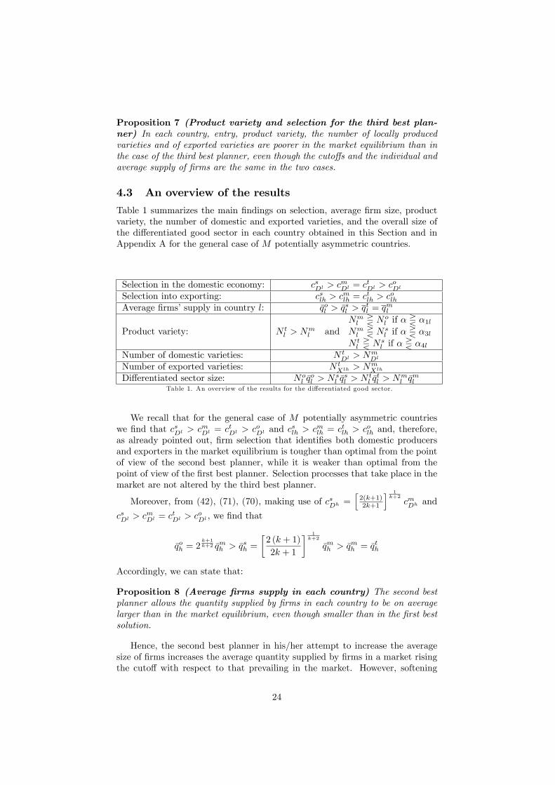
Following Melitz and Ottaviano (2008), we consider the case in which eachcountry, indexed by l = 1, ...,M , is populated by Ll consumers, each endowedwith one unit of labor. Preferences of consumers in l are defined over a contin-uum of differentiated varieties available in l that are indexed by i ∈ Ωl, and ahomogeneous good indexed by 0. All consumers in l indexed ε share the sameutility function given by

U l = qε0l + α

∫i∈Ωl

qεl (i) di− 1

2γ

∫i∈Ωl

(qεl (i))2di− 1

2η

(∫i∈Ωl

qεl (i) di

)2

(1)

with positive demand parameters α, η and γ, the latter measuring an inversemeasure of the ‘love for variety’as it represents the degree of product differen-tiation, and the others measuring the preference for the differentiated varietieswith respect to the homogeneous good. More precisely, α represents the inten-sity of preferences for the differentiated good relative to the homogeneous goodand η represents the degree of nonseparability across the differentiated varieties.The initial individual endowment ql0 of the homogeneous good is assumed to belarge enough for its consumption to be strictly positive in each country at themarket equilibrium and optimal solutions.Labor is the only factor of production. It is employed for the production of

the homogeneous good under constant returns to scale with unit labor require-ment equal to one. It is also employed for the production of the differentiatedvarieties. The technology requires a preliminary R&D effort of f l > 0 units oflabor in country l to design a new variety and its production process, whichis also characterized by constant returns to scale. The R&D effort cannot berecovered resulting in a sunk setup (‘entry’) cost. The R&D effort leads to thedesign of a new variety with certainty whereas the unit labor requirement c ofthe corresponding production process is uncertain, being randomly drawn froma continuous distribution with cumulative density

Gl(c) =

(c

clM

)k, c ∈ [0, clM ] (2)

This corresponds to the empirically relevant case in which marginal productivity1/c is Pareto distributed with shape parameter k ≥ 1 over the support [1/clM ,∞)for country l. Hence, as k rises, density is skewed towards the upper bound ofthe support of Gl(c). Notice that the scale parameter clM determines the level of‘richness’, defined as the measure of different unit labor requirements that canbe drawn within a country. Larger clM leads to a rise in heterogeneity along therichness dimension and to a reduction in the comparative advantage of countryl as it becomes possible to draw also larger unit labor requirements than theoriginal ones. The shape parameter k is an inverse measure of ‘evenness’, thatis of the similarity between the probabilities of different draws of c to happen.When k = 1, the unit labor requirement distribution is uniform on [0, clM ] withmaximum evenness.6 As k decreases, the unit labor requirement distributionbecomes less concentrated at higher unit labor requirements close to clM andevenness increases leading to a rise in heterogeneity along this dimension making

6When k tends to infinity, the distribution becomes degenerate at clM with all drawsdelivering a unit labor requirement clM with probability one.

5

low unit labor requirements more likely. Accordingly, more richness (larger clM )comes with higher average unit labor requirement (‘cost-increasing richness’),more evenness (smaller k) comes with lower average unit labor requirement(‘cost-decreasing evenness’).Countries are allowed to potentially differ not only in their size Ll, but also

in terms of their technology with country l having a comparative advantage(disadvantage) with respect to country h = 1, ...,M in the differentiated goodsector if clM is smaller (larger) than chM , and differences allowed also in the f

l

units of labor required for the preliminary R&D effort in country l. Moreover,differentiated varieties are traded at an iceberg trade cost that can differ bothacross and within countries. Specifically, we assume that τ lh units of the goodhave to be produced and shipped from the production country l to sell one unitin the destination country h, and ρlh ≡

(τ lh)−k ∈ (0, 1] measures the ‘freeness

of trade’for exports from l to h. As within country trade may not be costlessdue to domestic trade costs τ ll, we assume that ρll ≡

(τ ll)−k ∈ (0, 1]. The

homogenous good is, instead, assumed to be freely traded.Given that we allow for a potentially asymmetric multi-country framework,

we will try to understand how the differences in terms of the dimension ofthe domestic market (‘home market effect’), of technology and comparativeadvantage (‘development’) and market access due to trade barriers (‘geography’)and number of trading countries (‘globalization’) affect the intensity of marketdistortions.

2.1 Market equilibrium and first best optimum

We present now the free market equilibrium and then the allocation of theresources determined by a first best global planner maximizing global welfareconstrained only by technology and endowments.

2.1.1 The market outcome

In the decentralized equilibrium, within each country, consumers maximize util-ity under their budget constraints, firms maximize profits given their techno-logical constraints, and all markets clear. It is assumed that the labor marketas well as the market of the homogeneous good are perfectly competitive. Thehomogeneous good is chosen as numeraire and this, together with its produc-tion technology and the fact that it is freely traded, implies that the wage ofworkers equals one in all countries. The market of differentiated varieties is,instead, monopolistically competitive with a one-to-one relation between firmsand varieties and consumers buy both locally produced and imported varieties.The first order conditions for utility maximization give individual inverse

demand for variety i in l as

pl (i) = α− γqεl (i)− ηQεl (3)

whenever qεl (i) > 0, with pl (i) denoting the price of variety i in l, and Qεl =∫i∈Ωl q

εl (i) di representing the individual aggregate demand in l of differentiated

varieties.Aggregate demand for each variety i in country l can be derived from (3) as

ql (i) ≡ Llqεl (i) =αLl

ηNl + γ− Ll

γpl (i) +

ηNlηNl + γ

Ll

γpl, ∀i ∈ Ωl∗ (4)

6

where the set Ωl∗ is the largest subset of Ωl such that demand in l is positive,Nl is the measure (‘number’) of varieties in Ωl∗, that is given by the sum ofdomestic and imported varieties sold in l, and pl = (1/Nl)

∫i∈Ωl

∗pl (i) di is their

average price. Variety i belongs to this set when

pl (i) ≤1

ηNl + γ(γα+ ηNlpl) ≡ plmax (5)

where plmax ≤ α represents the price at which demand for a variety in l is drivento zero.7

The aggregate consumption in country h of a variety that is produced in lwith productivity 1/c is

qlh(c) = qεlh(c)Lh

where qεlh(c) is the individual consumption of that variety. Note that when twosuffi xes are used, the first one denotes the production country while the secondone the country in which the good is consumed.The quantity qlh(c) is obtained by

maxqlh(c)

πlh(c) =[plh(c)− τ lhc

]qlh(c)

subject to its aggregate inverse demand in h, that is

plh(c) = α− γ

Lhqlh(c)− η

LhQmh

where ‘m’labels equilibrium variables and Qmh ≡∑Mj=1

(N jE

∫ cjM0

qjh(c)dGj(c))

represents the total supply of differentiated varieties available in the market incountry h with N j

E denoting the number of firms entering in country j.The corresponding first order conditions for profit maximization are satisfied

by

qmlh(c) =

Lh

2γ τlh (cmlh − c) if c ≤ cmlh ≡

phmaxτ lh

= 1τ lh

(α− η

LhQmh)

0 if c > cmlh(6)

Expression (6) defines a cutoff rule as only entrants in country l that areproductive enough (c ≤ cmlh) sell their variety in country h. For them, theprice set in h that corresponds to the profit-maximizing quantity qmlh(c) ispmlh(c) = τ lh (cmlh + c) /2, implying a markup on sales in h equal to µmlh(c) =pmlh(c)− τ lhc = τ lh (cmlh − c) /2 and maximized profits are given by

πlh(c) =Lh

4γ

(τ lh)2

(cmlh − c)2 (7)

Notice that sales in the domestic market can be obtained considering h = l. Inthis case, the domestic cutoff cmll is also denoted by c

mDl .

7Melitz and Ottaviano (2008) show that rewriting the indirect utility function in terms ofaverage price and price variance reveals that it decreases with average prices p, but rises withthe variance of prices σ2p (holding p constant), as consumers then re-optimize their purchasesby shifting expenditures towards lower priced varieties as well as the numeraire good. Notealso that the demand system exhibits ‘love of variety’: holding the distribution of pricesconstant (namely holding the mean p and variance σ2p of prices constant), utility rises withproduct variety N .

7

Expression (6) implies that for all marginal firms selling in h we haveτ lhcmlh = τhhcmDh = phmax . Hence, the relationship among cutoffs for firmsselling in h is such that

cmlh =τhh

τ lhcmDh ∀l, h = 1, ....,M (8)

Due to free entry and exit condition, in equilibrium expected profit of firmsproducing in l is exactly offset by the sunk entry cost f l and, therefore,

M∑h=1

∫ cmlh

0

Lh

4γ

(τ lh)2

(cmlh − c)2dGl(c)

= f l (9)

Given (2), (7) and (8), the ‘free entry condition’can be rewritten as

M∑h=1

Lhρlh(τhhcmhh

)k+2= 2γ (k + 2) (k + 1)

(clM)kf l (10)

This expression, together with the analogous expressions holding for all otherM − 1 countries, yields a system of M equations that, making use of Cramer’srule, can be solved for the M equilibrium domestic cutoffs given by

cmDl =1

τ ll

2γ (k + 1) (k + 2)

Ll

M∑h=1

[fh(chM)k |Chl|]

|P |

1

k+2

∀l = 1, ...,M (11)

where |P | is the determinant of the trade freeness matrix

P =

ρ11 ρ12 · · · ρ1M

ρ21 ρ22 · · · ρ2M

· · · · · · . . . · · ·ρM1 ρM2 · · · ρMM

and |Chl| is the cofactor of its ρhl element.8In general, the total number of varieties consumed in country l is given by the

sum of domestic and of imported varieties from all trading partners. Specifically,the number of varieties produced in h and consumed in l is derived from theselection conditions and is given by

Nhl = NhEG

h(chl) (12)

The total number of varieties consumed in country l (Nl) is

Nl =

M∑h=1

Nhl (13)

8Notice thatM∑h=1

[fh(chM)k |Chl|] > 0 ∀l = 1, ...,M has to be satisfied also to have a

positive production for domestic consumers in all countries for the market solution.

8

Given (12), (2) and (8), product variety Nl in (13) can be rewritten in thecase of the market equilibrium as follows

Nml =

(τ llcmDl

)k M∑h=1

ρhlNhE

(1

chM

)k(14)

Moreover, as the average price in country l is

pml =2k + 1

2 (k + 1)τ llcmDl , (15)

it can be combined with the price threshold in (5) to express the number ofvarieties sold in l in the market equilibrium as

Nml =

2γ (k + 1)

η

(α− τ llcmDl

)τ llcm

Dl

(16)

Hence, Nml in (16) can be equalized to Nm

l in (14) to get

M∑h=1

(ρhlNh

E

1(chM)k)

=2γ (k + 1)

η

(α− τ llcmDl

)(τ llcm

Dl

)k+1

This gives a system ofM linear equations that using Cramer’s rule can be solvedfor the number of entrants in the M countries

N lmE =

2γ (k + 1)(clM)k M∑

h=1

[(α−τhhcm

Dh)(τhhcm

Dh

)k+1 |Clh|]

η |P | ∀l = 1, ...,M (17)

which, as the domestic cutoffs in (11) and the cutoffs for exporting firms derivedmaking use of (8), is affected by parameters determining the technology ofproduction available in each country and by comparative advantage, as well asby the market size of each country, the number of trading countries and thelevel of trade costs.9

2.1.2 The first best optimum

Let us now consider the problem faced by a social planner who can allocatethe resources available within each country to design a specific number of newvarieties, with the corresponding unit labor requirement c uncertain, and tothe production of only a specific subset of these potentially available varietiestogether with the homogenous good.The quasi-linearity of (1) implies transferable utility. Thus, social welfare

may be expressed as the sum of all consumers’utilities in all M countries. Thisimplies that the first best (‘unconstrained’) planner chooses the number of vari-eties and their output levels so as to maximize the total social welfare function

9Notice that in the example of two trading countries with no internal trade costs andcommon sunk entry cost f that will be presented later on in Section 5.1.1, the conditions thathave to be satisfied to have positive values for both N1m

E and N2mE , imply that cm12 < cm

D1 andcm21 < cm

D2 , so that only a subset of relatively more productive firms export in the market.

9

given by the sum of aggregate utility of all countries obtained for each coun-try multiplying individual utility in (1) for the number of consumers Ll. Thismaximization is subject to the resource constraints, the varieties’productionfunctions and the stochastic ‘innovation production function’(i.e. the mecha-nism that determines each variety’s unit labor requirement as a random drawfrom Gl(c) after f l units of labor have been allocated to R&D) that hold for allcountries.In other words, the planner maximizes the utility derived by all consumers

living in the M countries from the consumption of the homogeneous good andof the differentiated varieties that are both those domestically produced andthose imported. Specifically, the utility of all Ll workers living in country l isgiven by

W l(Ll) = qε0lLl + α

M∑h=1

[NhE

∫ chM

0

qεhl(c)LldGh(c)

]+ (18)

−γ2

1

Ll

M∑h=1

[NhE

∫ chM

0

[qεhl(c)L

l]2dGh(c)

]+

−η2

1

Ll

M∑h=1

[NhE

∫ chM

0

qεhl(c)LldGh(c)

]2

,

Thus, the planner maximizes the ‘global’utility which is given by

W =

M∑l=1

W l(Ll) =

M∑l=1

qε0lLl + α

M∑l=1

M∑h=1

[NhE

∫ chM

0

qεhl(c)LldGh(c)

]+(19)

−γ2

M∑l=1

1

Ll

M∑h=1

[NhE

∫ chM

0

[qεhl(c)L

l]2dGh(c)

]+

−η2

M∑l=1

1

Ll

[M∑h=1

(NhE

∫ chM

0

qεhl(c)LldGh(c)

)]2

with respect to consumption of the homogeneous goods in each country, thequantities produced for consumption in all countries by all firms in the differ-entiated good sector and the number of entrants in all countries, subject to theresource constraints, the firm production functions and the stochastic ‘varietyproduction function’expressed in the selection conditions (12) that hold for allM countries.From the resource constraint of country l, the supply of the homogenous

good in country l is given by

Ql0 = ql0Ll + Ll − f lN l

E −N lE

M∑h=1

[∫ clM

0

τ lhcqεlh(c)LhdGl(c)

](20)

This implies that the supply of the homogeneous good in country l (Ql0) is givenby the sum of total local endowments of the good (ql0L

l) and its local productionobtained employing labour units locally available (Ll) once subtracted thoseemployed, respectively, to undertake the local R&D investment (f lN l

E) and to

10

produce the differentiated varieties sold in the local and in the foreign countries

(N lE

∑Mh=1

[∫ clM0

τ lhcqεlh(c)LhdGl(c)]).

The condition that the global supply of the homogenous good is equal to itsglobal demand requires that

M∑l=1

Ql0 =

M∑l=1

qε0lLl (21)

which, making use of (20), implies

M∑l=1

qε0lLl =

M∑l=1

ql0L

l + Ll − f lN lE −N l

E

M∑h=1

[∫ clM

0

τ lhcqεlh(c)LhdGl(c)

](22)

Substituting (22) into (19), and making use of qlh(c) = qεlh(c)Lh, the plannermaximizes

W =

M∑l=1

W l(Ll) = (23)

=

M∑l=1

ql0L

l + Ll − f lN lE −N l

E

M∑h=1

[∫ clM

0

τ lhcqlh(c)dGl(c)

]+

+α

M∑l=1

M∑h=1

[NhE

∫ chM

0

qhl(c)dGh(c)

]+

−γ2

M∑l=1

1

Ll

M∑h=1

[NhE

∫ chM

0

[qhl(c)]2dGh(c)

]+

−η2

M∑l=1

1

Ll

[M∑h=1

(NhE

∫ chM

0

qhl(c)dGh(c)

)]2

with respect to the quantities produced for all markets by all firms and thenumber of entrants in all countries, that is with respect to qij(c)∀c and N i

E withi, j = 1, ....,M .10

The first order conditions obtained for the quantity of a variety producedwith productivity 1/c in country i and consumed in j is

∂W

∂qij(c)= 0 ∀c

(α− τ ijc

)N iE −

γ

LjN iEqij(c)−

η

Lj

[M∑h=1

(NhE

∫ chM

0

qhj(c)dGh(c)

)]N iE

dGi(c) = 0 ∀c

10More precisely, in addition to the first order conditions written with respect to qij(c)∀cand N i

E , the first best planner should also consider the first order condition with respect tothe cutoffs. However, making use of the Pareto distribution in (2), it can be shown that thefirst order conditions with respect to the cutoffs becomes redundant because they identify thesame cutoffs as those derived from the first order condition with respect to qij(c) given inexpression (24).

11

that making use of the total quantity consumed in country j, that is Qoj ≡∑Mh=1

(NhE

∫ chM0

qhj(c)dGh(c)

), can be rewritten as

α− τ ijc− γ 1

Ljqij(c)− η

1

LjQoj = 0

Hence, for quantities produced in l to be consumed in h the planner followsthe rule

qolh(c) =

Lh

γ τlh (colh − c) c ≤ colh with colh ≡ 1

τ lh

(α− η 1

LhQoh)

0 c > colh(24)

where ‘o’labels first best optimum variables. Results in (24) reveal that, justlike the market, also the planner follows M cutoff rules, one for each country,allowing only for the production in country l for consumption in country h ofthose varieties whose unit labor requirements are low enough with c ≤ colh. Itcan be readily verified from (24) that the first best output levels would clearthe market in the decentralized scenario only if each producer in l priced thequantities sold in h at its own marginal cost, that is only if plh(c) = τ lhc.Indeed, from the inverse demand function, we know that plh(c) = α− γ

Lhqlh(c)−

ηLhQoh = τ lhcolh −

γLhqlh(c) that, together with plh(c) = τ lhc, implies qlh(c) =

Lh

γ τlh (colh − c).The definitions of the cutoffs in (24) imply that the relationships between

the optimal cutoffs for all marginal firms selling in h are such that

colh =τhh

τ lhcoDh ∀l, h = 1, ....,M (25)

which are the same as those for the market equilibrium in (8), even though thecutoffs are different. Therefore, we can state that

Proposition 1 (Principle of no discrimination) There is no discrimina-tion of the first best planner with respect to the market equilibrium in favour ofdomestic or imported varieties.

The cutoffs of the unconstrained planner are derived in Appendix A from thefirst order conditions for the maximization of (23) with respect to the numberof entrants in each country i (that is from ∂W

∂NiE

= 0) and are given by

coDl =1

τ ll

γ (k + 1) (k + 2)

Ll

M∑h=1

[fh(chM)k |Chl|]

|P |

1

k+2

∀l = 1, ...,M (26)

Notice thatM∑h=1

[fh(chM)k |Chl|] > 0 ∀l = 1, ...,M has to be satisfied also to

have a positive production for domestic consumers in all countries for the firstbest solution.

12

In Appendix A we derive also the optimal number of entrants in each countryas a function of the cutoffs, that is

N loE =

γ (k + 1)(clM)k M∑

h=1

[(α−τhhco

Dh)(τhhco

Dh

)k+1 |Clh|]

η |P | ∀l = 1, ...,M (27)

Finally, making use of (12), for each country l the optimal number of domesticvarieties is No

Dl = Gl(coDl)NloE and the optimal number of exported varieties to

country h is NoXlh = Gl(colh)N lo

E .11

3 Equilibrium vs. optimum

There are different dimensions along which the effi ciency of the market outcomecan be evaluated, such as: the (conditional) cost distribution of firms producingand exporting the different varieties as dictated by the cutoff cmlh and the numberof varieties available for consumption in each country (product variety). In turn,the cost distributions determine the effi ciency of the corresponding distributionsof firm sizes, domestic production and exports. Moreover, it contributes indetermining the effi ciency of the overall dimension of the differentiated goodssector in the market of each country (i.e. total supply of differentiated varieties),the mass (number) of firms that undertake the initial R&D effort entering ineach market, and the number of firms that survive producing the differentiatedvarieties for the domestic and the foreign consumers.At the origins of the ineffi ciencies of the market equilibrium is the fact that

consumers in each country value variety and monopolistically competitive firmsheterogeneous in their productivity levels are price setters. Setting their pricefor each locality with a markup over their marginal cost, firms reduce the averagequantity that consumers buy within each of these locations with respect to theaverage quantity that they would have purchased if differentiated varieties hadbeen sold at their marginal cost.12

As shown in the last part of Appendix A, most of the evaluations in termsof effi ciency of the market outcome can be obtained for the general case ofasymmetric countries. In this Section, we use the results derived in AppendixA to compare the equilibrium outcome with the optimal unconstrained solutionalong different dimensions such as: selection processes that identify firms thatsurvive producing for domestic and foreign consumers; individual and overallaverage size of firms in the differentiated good sector; product variety availablefor consumption and entry of innovating firms in each country. These results arefirst presented in the case of M symmetric trading countries facing no internaltrade costs and, then, in the case in which countries differ in terms of thesize of their domestic market (Ll), technology that defines their comparative

11Notice that in the case of two countries with no internal trade costs and common sunkentry cost f considered in Section 5.1.1, the conditions that have to be satisfied to havepositive values for both N1o

E and N2oE , imply that co12 < co

D1 and co21 < co

D2 , so that in eachcountry only a subset of relatively more productive firms export in the optimal solution.12The tradeoffs the first best planner faces when firms are monopolistically competitive and

heterogeneous are discussed in Nocco, Ottaviano and Salto (2014) for the closed economy.Specifically, see expression (8) at page 306 in Nocco, Ottaviano and Salto (2014) and thesubsequent comments.

13

advantage (clM ) and the fl units of labor required for the preliminary R&D

effort, and, finally, trade barriers (τ lh) that identify their accessibility in eachcountry/locality.

3.1 The case of symmetric countries

Let us first consider the case of M perfectly symmetric trading countries with-out internal trade costs (that is with τ ll = 1 implying ρll = 1∀l = 1, ...,M) toevaluate how the intensity of market distortions is affected by different phenom-ena such as: a process of ‘globalization’that increases the number of tradingcountries /M ; ‘demographic growth’and processes that increase the size of eachcountry L allowing to evaluate ‘home market effects’; ‘international economicintegration’that reduces trade barriers increasing the freeness of trade ρ; im-provements in the technology available within each country (‘development’) thatreduce the highest cost draw cM or the entry/innovating cost f , or, eventually,increase the chances of having a high productivity draw reducing the shape pa-rameter k. Recall that while a smaller cM reduces heterogeneity along the cost-richness dimension implying lower average unit labor requirement, a smaller kincreases heterogeneity along the evenness dimension reducing the average unitlabor requirement.Notice that all the results discussed in the case of symmetric countries are

consistent with those of a closed economy, which can be obtained with M = 1and/or ρ = 0, presented in Nocco, Ottaviano and Salto (2013, 2014).

3.1.1 Selection and firm size

In the case of perfectly symmetric countries,13 τ lh = τ and ρlh = ρ∀l, h =

1, ....,M imply |P | = [1 + (M − 1)ρ] (1− ρ)M−1 and

M∑h=1

[|Chl|] = (1− ρ)M−1,

and therefore the market equilibrium domestic cutoffs in (11) can be rewrittenas

cmD =

2γ (k + 1) (k + 2) fckM

[1 + (M − 1)ρ]L

1k+2

(28)

and the first best domestic cutoffs in (26) as

coD =

γ (k + 1) (k + 2) fckM

[1 + (M − 1)ρ]L

1k+2

(29)

Comparing the equilibrium domestic cutoff in (28) with the optimal one in(29) reveals that cmD = 21/(k+2)coD, which implies c

oD < cmD . Accordingly, vari-

eties with c ∈ [coD, cmD ] should not be supplied in the domestic market. Moreover,

differences in the strength of selection translate also into the export status. Inparticular, comparing expressions (28) with (29) together with (8) and (25),reveals that the cutoffs for exporting firms (denoted as cX when countries aresymmetric) are such that cmX = 21/(k+2)coX , which implies c

oX < cmX . Accord-

ingly, varieties with c ∈ [coX , cmX ] should not be exported or, equivalently, looking

this phenomenon from the other side of the coin, should not be imported byother countries.13Recall that in all this subsection, we consider the case in which there are no domestic

trade costs.

14

The intuition behind the causes at the origin of these ineffi ciencies is that,in the market equilibrium, firms are price setters and a firm with marginal costc producing in l sets the price for its variety sold in h with a markup over itsmarginal cost that is equal to µmlh(c) = τ lh (cmlh − c) /2. This implies that theprices of differentiated varieties are ineffi ciently high within each country withrespect to the price of the numeraire good and, consequently, this biases theconsumption in favor of the homogeneous good softening the selection processamong the producers of the differentiated varieties.

The results on optimal selection processes have also implications in terms ofoptimality of the firm size distribution of domestic and exporting firms. Adapt-ing to the specific case of M symmetric countries the general results derived inthe final part of Appendix A for asymmetric countries, we find that, with re-spect to the optimum, the market equilibrium undersupplies varieties producedwith marginal cost c ∈ [0,

(2− 21/(k+2)

)coD), and oversupplies varieties with

marginal cost c ∈ ((2− 21/(k+2)

)coD, c

mD ] in the domestic countries. Moreover,

in the market equilibrium firms export a quantity that is smaller than optimalof varieties produced with marginal cost c ∈ [0,

(2− 21/(k+2)

)coX), and larger

than optimal of those produced with marginal cost c ∈ ((2− 21/(k+2)

)coX , c

mX ].

The intuition behind this can be explained by the fact that the markupµmlh(c) is a decreasing function of c and this implies that more productive firmsdo not pass on their entire cost advantage to consumers as they absorb part ofit in the markup. As a result, the price ratio of less to more productive firmsis smaller than their cost ratio and thus the quantities sold by less productivefirms are too large from an effi ciency point of view relative to those sold by moreproductive firms.

Moreover, the cutoff ranking implies that in the market not only the aver-age production of firms in each country for any of their destination country isineffi ciently low (as qmD < qoD and qmX < qoX), resulting in an ineffi ciently lowaverage firm size, but also that the average quantity supplied by all, domesticand foreign, firms within each country is smaller than optimal (as qm < qo).14

The intuition behind this is that the lower cutoff implied by marginal costpricing followed by the first best planner makes firms on average larger in theoptimum than in the market equilibrium.

Finally, the implications of the results and comparative statics in Appen-dix A allow us to state that the percentage gap in the cutoffs, in average firmsize and in the average quantity supplied within each country and the withinsector misallocation that materializes as the overprovision of high cost varietiesand underprovision of low cost varieties are not affected by any of the follow-ing processes: ‘globalization’that increases the number of trading countries /M ;‘demographic growth’that increases the home market size L of each country; ‘in-ternational integration’that reduces trade barriers increasing ρ; ‘development’that improves the technology available within each country reducing cM and/or

14Again, these results are obtained adapting the more general ones for asymmetric countriesin (69), (70) and (71) presented in the last part of Appendix A. Notice that when countriesare symmetric we avoid in the variable the suffi x that denotes the country (i.e. we use qm

instead of qmh ).

15

the entry cost f . Instead, more heterogeneity due to more cost-decreasing even-ness, that is a smaller k that implies a higher chance of having high productivitydraws: leads to a larger percentage gap in the cutoffs between the market equi-librium and the optimum; makes the overprovision of varieties relatively morelikely than its underprovision in the market equilibrium and decreases the per-centage gap in the average production of firms in each country for their domesticand foreign markets and in the average quantity supplied by all firms within eachcountry.

3.1.2 Size of the differentiated sector, product variety and entry

Adapting the general results in (72) and (73) in Appendix A, we find that,also in the specific case of M symmetric countries, coD < cmD implies that themarket misallocate resources between sectors as the total supply of differentiatedvarieties is smaller than optimal in each country (that is, Nmqm < Noqo).In this case, the percentage gap in the total output of differentiated varietiesbetween the market equilibrium and the optimum is

Noqo −Nmqm

Noqo=cmD − coDcoD

coDα− coD

where (cmD − coD)/coD is only affected by k, which, together with γ, L, M , f andcM , affects also coD/ (α− coD).Specifically, as larger values of the market size L, of the number of trading

countriesM and of the freeness of trade ρ, and smaller values of γ, f and cM de-crease coD/ (α− coD), they imply smaller values for the ratio (Noqo −Nmqm) /Noqo.Moreover, we find that there can exist a threshold value of k, k∗,15 such thatmore cost-decreasing evenness decreases the gap in the total output of the dif-ferentiated varieties between the market equilibrium and the optimum if k > k∗

and, viceversa, it increases the gap if k < k∗. The threshold value k∗ increaseswith L, M , ρ and cM , and decreases with γ and f . However, if L, M , ρ and cMare suffi ciently small and/or γ and f are suffi ciently large, more cost-decreasingevenness does always decrease the gap.Consequently, we can state what follows:

Proposition 2 With M symmetric countries, the total supply of differentiatedvarieties in the market equilibrium is smaller than optimal in all locations. Thisgap is smaller (larger): in larger overall economies due to larger (smaller) homemarkets, more (less) integrated countries or to a larger (smaller) number oftrading countries, in more (less) developed economies that benefit from better(worse) available technologies, lower (larger) entry costs and higher (smaller)chances of having low cost firms, and in countries in which varieties are closer(farther) substitutes. More cost-decreasing evenness decreases the gap if k > k∗

and, viceversa, it increases the gap if k < k∗.15More precisely, more cost-decreasing evenness increases the gap if[

21

k+2 ln 2− (2k + 3)(

21

k+2 − 1)/ (k + 1)

]/(

21

k+2 − 1)

+ ln [(k + 1)(k + 2)] >

ln

[1 + (M − 1)ρ]Lc2M/ (γf); viceversa, it decreases the gap if the opposite inequal-

ity sign holds. The threshold k∗ corresponds to the value at which the function[2

1k+2 ln 2− (2k + 3)

(2

1k+2 − 1

)/ (k + 1)

]/(

21

k+2 − 1)

+ ln ((k + 1)(k + 2)), which is

increasing in k, crosses ln

[1 + (M − 1)ρ]Lc2M/ (γf), and it exists only if L, M , ρ and cM

are suffi ciently large and/or γ and f are suffi ciently small.

16

Hence, increases in the overall size of the economy due to ‘globalization’,‘demographic growth’and ‘economic integration’and processes of ‘development’that reduce cM or f , decrease the percentage gap in the total output of thedifferentiated varieties between the market equilibrium and the optimum.

Turning to the mass (number) of varieties supplied respectively in the do-mestic and in the M − 1 foreign markets, they are, respectively, given by

NmD =

2γ (k + 1)

η [1 + (M − 1)ρ]

(α− cmD)

cmDand Nm

X = ρ2γ (k + 1)

η [1 + (M − 1)ρ]

(α− cmD)

cmD(30)

while their optimal values correspond to

NoD =

γ (k + 1)

η [1 + (M − 1)ρ]

(α− coD)

coDand No

X = ργ (k + 1)

η [1 + (M − 1)ρ]

(α− coD)

coD(31)

Comparing the number of domestic and exported varieties in (30) and (31), andoverall product variety available within each country from (16) and (67), wefind that cmD = 21/(k+2)coD implies N

mD > No

D, NmX > No

X and Nm > No as long

as

α > α1 ≡1

2k+1k+2 − 1

coD =1

2k+1k+2 − 1

γ (k + 1) (k + 2) fckM

[1 + (M − 1)ρ]L

1k+2

(32)

which is the case when α as well as L, M and ρ are large and when γ, cM , fand k are small. On the contrary, Nm

D < NoD, N

mX < No

X and Nm < No whenα < α1.Turning to entry, the equilibrium number of entrants in (17) can be rewritten

in the case of symmetric countries as

NmE =

2γ (k + 1) ckMη [1 + (M − 1)ρ]

(α− cmD)

(cmD)k+1

while that for the first best planner in (27) as

NoE =

γ (k + 1) ckMη [1 + (M − 1)ρ]

(α− coD)

(coD)k+1

These can be used to show that cmD = 21/(k+2)coD implies NmE > No

E as long as

α > α2 ≡22/(k+2) − 1

21/(k+2) − 1coD =

22/(k+2) − 1

21/(k+2) − 1

γ (k + 1) (k + 2) fckM

[1 + (M − 1)ρ]L

1k+2

> α1

(33)which is the case when α as well as L, M and ρ are large and when γ, cM , fand k are small. On the contrary, Nm

E < NoE when α < α2.

In summary, we can state that

Proposition 3 In the case of M symmetric countries, entry, overall productvariety and the number of domestic and imported varieties are larger (smaller)in the market equilibrium than in the optimum when market size is large (small),the number of trading countries is large (small), their level of integration is high(low), varieties are close (far) substitutes, the sunk entry cost is small (large),the difference between the highest and the lowest possible cost draws is small(large), and the chances of having low cost firms are large (small).

17

This has interesting implications for the impact of increases in the overalldimension of the economy driven by different channels such as: internationalintegration processes that increases ρ, globalization processes that increase thenumber of trading countries and/or demographic growth or other processes thatincrease the home market size. Moreover, it has also interesting implicationsfor the impact of economic development that reduce the highest cost draw cMor the entry/innovating cost f , or, eventually, increase the chances of havinga high productivity draw reducing the shape parameter k. Indeed, startingfrom suffi ciently small levels of the overall size of the economy and/or levels ofdevelopment of the technologies, increases in one or both of these levels (due toincreases in ρ, L andM or to decreases in cM , f and k) can switch the countriesfrom a situation in which α < α1 to one in which α > α1, decreasing α1. Then,this would cause the transition from a situation in which product variety, thenumber of domestic and exported varieties are ineffi ciently poor in each country(Nm < No, Nm

D < NoD and Nm

X < NoX) to a situation in which they become

ineffi ciently rich (Nm > No, NmD > No

D and NmX > No

X).As larger overall sizes of the economies and technology improvements reduce

α2, they may well cause the transition from a situation in which the resourcesdevoted to develop new varieties are ineffi ciently small in each country (Nm

E <NoE) to a situation in which they are ineffi ciently large (N

mE > No

E). Given that(32) and (33) imply α1 < α2, the market provides too little entry with too littlevariety in each country for α < α1 and too much entry with too much varietyin each country for α > α2. For α1 < α < α2 it provides, instead, too muchvariety and too little entry.

3.2 The case of asymmetric countries

Let us now turn to the case of M asymmetric countries to understand if theeffi ciency properties of the market change with respect to the case with Msymmetric countries.16

3.2.1 Selection and firm size

The analysis in Appendix A reveals that also in the general case ofM asymmet-ric countries, selection in the market equilibrium is weaker than optimal in eachcountry: varieties with c ∈ [coDl , c

mDl ] should not be supplied in domestic mar-

kets, and varieties with c ∈ [colh, cmlh] should not be exported by firms producing

in l to be consumed in country h.In turn, the cost distribution determines the effi ciency of the firm size distri-

bution and we find that resources are misallocated within the differentiated goodsector. Indeed, the results for the general case confirm those for symmetric coun-tries as, with respect to the optimum, the market equilibrium undersupplies ineach country h varieties produced in country l with low marginal cost, that is va-rieties produced with c ∈ [0,

(2− 21/(k+2)

)colh), and oversupplies varieties with

high marginal cost, that is varieties produced with c ∈ ((2− 21/(k+2)

)colh, c

mlh].

Finally, also in the general case of M asymmetric countries, the cutoff rank-ing colh < cmlh dictates the same average output ranking with the average quan-tities produced in each country for each destination and the average supply of

16For the analytical derivation of the results see the final part of Appendix A.

18

a variety in each country smaller than optimal in the market as qmlh < qolh andqmh < qoh.

Hence, summarizing the results discussed above for both the symmetric andasymmetric countries, we can state what follows:

Proposition 4 In the market equilibrium with respect to the optimum: firmselection in the production status for domestic and foreign countries is weakerthan optimal; high (low) cost firms oversupply (undersupply) their varieties in allcountries they are serving; both the average production of firms in each countryfor any of their destination country and the average quantity supplied by alldomestic and foreign firms within each country are smaller than optimal.

Moreover, from comparative statics in Appendix A we find that in generalfor both the cases of symmetric and asymmetric countries:

Proposition 5 The number of trading countries, the size of each economy,the technology available for the production of the modern differentiated goodsas determined by the upper-bound cost and the cost of innovation, and tradebarriers that affect the accessibility of other countries by exporting firms haveno impact on the overprovision or on the underprovision of varieties in bothdomestic and foreign countries and on the percentage deviation of the marketequilibrium from the optimum for domestic and export cutoffs, for the averagesupply of firms in each of their destination country and for the average quantitysupplied by all firms within each country. However, more heterogeneity amongfirms due to more (less) cost-decreasing evenness that reduces (increases) k,increases (decreases) the percentage gaps in the cutoffs, makes the overprovisionof high cost varieties relatively more (less) likely than its underprovision in themarket equilibrium and decreases (increases) the percentage gap in average firmsize and in the average quantity supplied by all firms within each country.

3.2.2 Size of the differentiated sector, product variety and entry

The ranking of the domestic cutoffs coDh < cmDh is also responsible of the rankingof the overall size of the differentiated good sector that is smaller than optimalin the market in each country as No

hqoh > Nm

h qmh . Moreover, the ratio (No

hqoh −

Nmh q

mh )/No

hqoh is affected by k as well as by the technology available in all

countries for the production of the modern differentiated goods as determinedby the upper-bound costs and the cost of innovation, and by the number oftrading countries and their accessibility to other localities as defined by trade

barriers, that is by all factors affecting the termM∑h=1

[fh(chM)k |Chl|] / |P |.

Turning to product variety, Noh in (67) can be used to evaluate the number

of product supplied in the market in (16). In this case Noh and N

mh can not

be ranked unambiguously. More precisely, as cmDh = 21/(k+2)coDh we have that

19

Nmh > No

h when

α > α1h ≡1

2k+1k+2 − 1

τhhcoDh =1

2k+1k+2 − 1

γ (k + 1) (k + 2)

Lh

M∑l=1

[f l(clM)k |Clh|]

|P |

1

k+2

which is the case when α as well as Lh are large and when γ and the termM∑h=1

[fh(chM)k |Chl|] / |P | are small. On the contrary, Nm

h < Noh when α < α1h.

In the general case of asymmetric countries, the comparison between N loE

in (27) and N lmE in (17), and, consequently the comparison between exported

and domestic varieties determined by the first best planner and the market,

is complicated by the presence of the summation (M∑h=1

) in the numerator of

the solutions. Specifically, while the terms in the summation are smaller in themarket and this works in favour of having less entry in the market (N lm

E < N loE ),

the numerator of the solution for the market has a 2 in the numerator that, onthe contrary, works in favour of having more entry in the market (N lm

E > N loE ).

This captures two contrasting effects present in the market, that were alreadydescribed by Spence (1976). Indeed, adapting his words to this specific case,revenues in the market may fail to cover the costs of a socially desirable productbecause of setup costs, while they could be covered by a social planner who couldallow for production at a loss. This produces a force that tends to produce inthe market less entry (and product variety) than optimal. On the other hand,as firms in the market hold back output setting their price above their marginalcost, they leave more room for entry than would marginal cost pricing that wouldbe followed by the first best planner decentralizing his/her choices, producing abusiness stealing effect that tends to generate more entry (and product variety)than optimal.

Finally, the number of domestic producers and of exporters in the market isclearly not optimal as No

Dl = Gl(coDl)NloE is different from Nm

Dl = Gl(cmDl)NlmE

and NoXlh = Gl(colh)N lo

E is different from NmXlh = Gl(cmlh)N lm

E . However, as forthe case of the number of firms entering the market, the comparison betweenthe two cases is not straightforward and requires to specify all the parametersof the model.

4 The constrained planners

We show in the next Section that the first best optimum can not be decentral-ized when differentiated production subsidies/taxes are not available. However,the constrained (second or third best) planner relies on a common productionsubsidy (eventually tax if it is negative) that in an open economy frameworkimplies that profits of a firm producing in h for l are

πhl(c) =[phl(c) + shl

]qhl(c)− τhlcqhl(c)

20

where shl is the specific common subsidy offered to firms producing in h to sellin l the quantity qhl(c).With inverse demand phl(c) = α − γ

Llqhl(c) − η

LlQl = plmax − γ

Llqhl(c) and

plmax = α− ηLlQl, profit from sales in l of a good produced in h can be rewritten

as

πhl(c) =[plmax + shl − γ

Llqhl(c)− τhlc

]qhl(c)

In this case, the first order condition for profit maximization with respect toqhl(c) holds for

qhl(c) =Ll

2γ

(plmax + shl − τhlc

)(34)

showing that, for a given plmax, a positive (negative) specific subsidy can be usedto increase (decrease) firm sales in l.The choke price pins down the highest marginal cost chl such that qhl(c) is

non-negativeplmax = τhlchl − shl (35)

so that we can rewrite the profit maximizing quantities in (36) as

qhl(c) =

Ll

2γ τhl (chl − c) c ≤ chl

0 c > chl(36)

and prices as

phl(c) =1

2τhl (chl + c)− shl (37)

Moreover, profits are given by

πhl(c) =Ll

4γ

(τhl)2

(chl − c)2 (38)

Notice that, while quantities in (36) and profits in (38) have the same ex-pression as in the market equilibrium given, respectively, in (6) and (7), pricesin (37) are affected by the subsidy.Finally, making use of the Pareto distribution in (2) and expressions (36),

the average production of firms in h for consumption in l for the constrainedplanners is

qhl =

∫ chl

0

qhl(c)dGlhl(c) =

Ll

2γ

1

(k + 1)τhlchl (39)

4.1 The second best planner

The second best planner is unable to choose the output level supplied by eachfirm to local consumers and eventually exported, but he/she can set the mini-mum amount of productivity required for firms to survive in the domestic marketand those required to export in each of the other countries and, finally, deter-mine the number of firms that operate in each country controlling the numberof R&D projects undertaken in each economy.Specifically, the second best planner chooses the number of R&D projects

(N lsE ) and the cutoffs for domestic production and for exports (c

slh with l, h =

21

1, ...,M) for each country l so as to maximize social welfare in (23) subject tothe profit maximizing quantity qhl(c) in (36) and the selection conditions in(12).In Appendix B we write the first order conditions and find the solutions for

the second best planner, showing that the relationship between the cutoffs forthe second best planner has to be the following

cslh =τhh

τ lhcsDh ∀l, h = 1, ....,M (40)

where ‘s’labels second best optimum variables. Thus, as the first best plannerin (25), also the second best planner does not alter the relationship between thecutoffs of the two types of marginal firms (domestic and foreign) selling in eachcountry that characterizes the market equilibrium (8). So, also for the secondbest planner holds the principle of no discrimination with respect to the marketequilibrium in favour of domestic or imported varieties stated in Proposition 1for the first best planner.Expression (40) together with (35) implies that the specific subsidy which

can be used to implement the solution by the second best planner requires

sil = sjl = sl ∀i, j, l = 1, ....,M (41)

To show this, we know from (35) that plmax = τ ilcil − sil = τ jlcjl − sjl thatmaking use of (40) can be rewritten as τ il τ

ll

τ ilcsDl − sil = τ jl τ

ll

τjlcsDl − sjl that

implies sil = sjl.

The expression for the cutoffs (78) in Appendix B, can be compared with the

corresponding expression for the market (11), showing that csDl =[

2(k+1)2k+1

] 1k+2

cmDl ,

which respectively implies csDl > cmDl and, using (8) and (40), that cshl > cmhl

given that cshl =[

2(k+1)2k+1

] 1k+2

cmhl. Accordingly, varieties with c ∈ [cmDl , csDl ] are

not supplied in the market, while they would be supplied by the second bestplanner. Furthermore, varieties with c ∈ [cmhl, c

shl] are not exported from country

h to country l in the market, while they would be exported by the second bestplanner.Expressions (39) and (40) can be used to compute the average quantity

supplied in each country h by all domestic and foreign firms in the case of thesecond best planner

qsh =

M∑l=1

Nslhq

slh

M∑l=1

Nslh

=Lh

2γ

1

k + 1τhhcsDh (42)

with qsh > qmh as csDh > cmDh . Thus, we have:

Proposition 6 (Selection and average supply for the second best plan-ner) Firm selection that identifies both domestic producers and exporters in themarket equilibrium is tougher than optimal from the point of view of the secondbest planner who extends the average supply of varieties in each country.

22

Finally, making use of (12), the number of domestic varieties set by thesecond best planner for each country l is Ns

Dl = Gl(csDl)NlsE , while the number

of exported varieties from l to country h is NsXlh = Gl(cslh)N ls

E .17

4.2 The third best planner

The third best planner in the open economy can not affect the profit maximizingchoices of firms in terms of quantities and prices but he/she can affect thenumber of firms that operate in each country in order to maximize the socialwelfare in (23).Hence, the third best planner maximizes W with respect to N i

E for eachcountry i = 1, ...,M subject to: i) the profit maximizing quantity qhl(c) in (36);ii) the selection conditions in (12); and, finally, the free entry conditions for eachcountry l in (9) that, with (8) implying the same relationship between domesticand foreign cutoffs for firms selling in a country, impose to the planner the samecutoffs of the market equilibrium given in (11).In other words, the third best planner makes use of the same relationship

between cil and cDl that applies between domestic and foreign cutoffs in themarket equilibrium. Indeed, the third best planner is unable to set any cutoffas he/she can not rely on lump sum instruments on firms, which, instead, areavailable for the second best planner. However, as the second best planner,the third best planner can use a specific common production subsidy for allquantities sold in country l by firms producing in different countries h. Thus,the third best planner uses the instrument sil = sjl = sl given in (41) thatimplies cil = τ llcDl/τ il.18

In Appendix B we write the first order conditions and find the solutions forN ltE given in expression (79) with ‘t’labeling third best optimum variables when

they differ from the corresponding market equilibrium values.19

Finally, comparing (79) with (17) reveals that N ltE > N lm

E . Moreover, giventhat N t

Dl = Gl(cmDl)NltE and that N t

Xlh = Gl(cmlh)N ltE , we find that N

mDl < N t

Dl

and that NmXlh < N t

Xlh , and comparing (46) obtained in the next subsectionwith (16) reveals that Nm

l < N tl .

Moreover, given that the third best planner sets the same cutoffs of themarket equilibrium, the average quantity supplied by firms producing in l forconsumers in h in (39) and the average quantity supplied in each country h by

all domestic and foreign firms qth =M∑l=1

N tlhq

tlh/

M∑l=1

N tlh, obtained making use of

(69) and (8), are the same as those of the market equilibrium, that is qthl = qmhland qth = qmh .Therefore, we can state that

17Notice that in the case of two countries with no internal trade costs and common sunkentry cost f , the conditions that have to be satisfied to have positive values for both N1s

E andN2sE in (76) in Appendix B, imply that cs12 < cs

D1 and cs21 < cs

D2 , so that in each countryonly a subset of relatively more productive firms export in the second best case.18To show this, we know from (35) that plmax = τ ilcil − sil = τ jlcjl − sjl that with

sil = sjl = sl becomes τ ilcil = τ jlcjl that with j = l implies cil = τ llcDl/τ il.19 In the case of two countries with no internal trade costs and common sunk entry cost f ,

the solutions N1tE and N2t

E are both positive when ct12 < ctD1 and c

t21 < ct

D2 , so that, as inthe market equilibrium, only a subset of relatively more productive firms export.

23

Proposition 7 (Product variety and selection for the third best plan-ner) In each country, entry, product variety, the number of locally producedvarieties and of exported varieties are poorer in the market equilibrium than inthe case of the third best planner, even though the cutoffs and the individual andaverage supply of firms are the same in the two cases.

4.3 An overview of the results

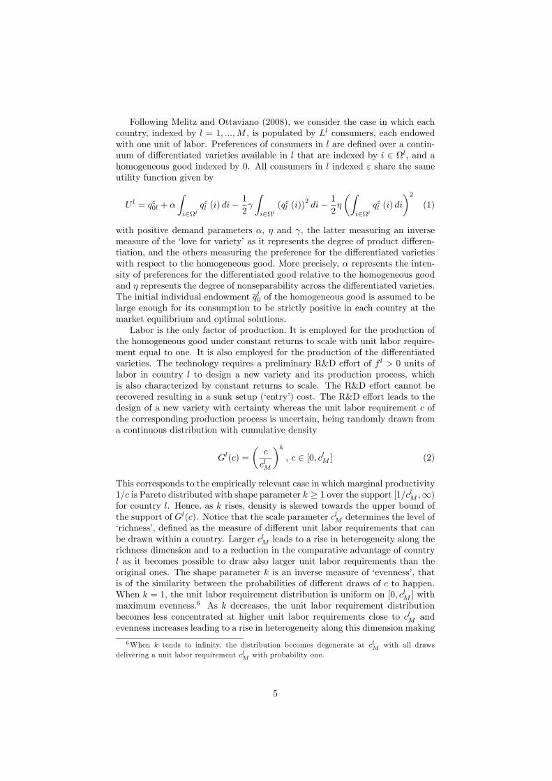
Table 1 summarizes the main findings on selection, average firm size, productvariety, the number of domestic and exported varieties, and the overall size ofthe differentiated good sector in each country obtained in this Section and inAppendix A for the general case of M potentially asymmetric countries.

Selection in the domestic economy: csDl > cmDl = ctDl > coDl

Selection into exporting: cslh > cmlh = ctlh > colhAverage firms’supply in country l: qol > qsl > qtl = qml

Product variety: N tl > Nm

l andNml R No

l if α R α1l

Nml R Ns

l if α R α3l

N tl R Ns

l if α R α4l

Number of domestic varieties: N tDl > Nm

Dl

Number of exported varieties: N tXlh > Nm

Xlh

Differentiated sector size: Nol qol > Ns

l qsl > N t

l qtl > Nm

l qml

Table 1. An overview of the results for the differentiated good sector.

We recall that for the general case of M potentially asymmetric countrieswe find that csDl > cmDl = ctDl > coDl and cslh > cmlh = ctlh > colh and, therefore,as already pointed out, firm selection that identifies both domestic producersand exporters in the market equilibrium is tougher than optimal from the pointof view of the second best planner, while it is weaker than optimal from thepoint of view of the first best planner. Selection processes that take place in themarket are not altered by the third best planner.

Moreover, from (42), (71), (70), making use of csDh =[

2(k+1)2k+1

] 1k+2

cmDh and

csDl > cmDl = ctDl > coDl , we find that

qoh = 2k+1k+2 qmh > qsh =

[2 (k + 1)

2k + 1

] 1k+2

qmh > qmh = qth

Accordingly, we can state that:

Proposition 8 (Average firms supply in each country) The second bestplanner allows the quantity supplied by firms in each country to be on averagelarger than in the market equilibrium, even though smaller than in the first bestsolution.

Hence, the second best planner in his/her attempt to increase the averagesize of firms increases the average quantity supplied by firms in a market risingthe cutoff with respect to that prevailing in the market. However, softening

24

competition also for less productive firms, he/she does not allow supply of firmsand thus firms’size to increase as much as in the first best case when, instead,the planner allows only more productive firms to increase their size, reducingthe production of less productive firms and stopping the production of the leastproductive ones.

Moreover, we know that the number of domestic and exported varieties andproduct variety is richer in the case of the third best planner than in the marketequilibrium.

Let us now compare the total consumption of differentiated varieties in acountry for the second and third best planners.20 To do this, we need to rewrite

the total quantity consumed in country l, Ql =∑Mh=1

(NhE

∫ chM0

qhl(c)dGh(c)

),

for the constrained planners making use of (36), (12), (13) and cil = τ llcDl/τ il

as

Ql =Ll

2γ

1

(k + 1)τ llcDlNl (43)

Moreover, for the second and third best planners plmax = α − ηLlQl with (35)

imply that in both cases the cutoffs have to satisfy the following relationship

α− η

LlQl = τhlchl − shl (44)

Then, in the specific case of the second best planner, we can rewrite (44) makinguse of (43), cil = τ llcDl/τ il, shl = sl and sl in (60) derived in the followingSection, to find

Nsl =

2γ (k + 1)

ητ llcsDl

(α− 1

2

2k + 1

k + 1τ llcsDl

)(45)

In the case of the third best planner, instead, shl =(sl)tgiven in (63) has to

be used, to get

N tl =

2γ (k + 1)

ητ llcmDl

(α− 1

2

2k + 3

k + 2τ llcmDl

)(46)

Hence, given (45), (46), (42) and qth = qmh in (70), we find that the total con-sumption of differentiated varieties in a country in the case of the second and of

the third best planner, respectively, evaluates toNsh qsh = Lh

η

α−

[2k+1

2(k+1)

] k+1k+2

τhhcmDh

and N t

hqth = Lh

η

[α− 2k+3

2(k+2)τhhcmDh

]. Comparing the dimensions of the differ-

entiated sector in all situations, we find that Noh qoh > Ns

h qsh > N t

hqth > Nm

h qmh .

21

20 In general, notice that Qh =∑Ml=1

(N lE

∫ clM0 qlh(c)dGl(c)

)=∑M

l=1

(N lEG

l (clh)∫ clh0 qlh(c)dGllh(c)

)=

∑Ml=1

(N lEG

l (clh) qlh)

=∑Ml=1 (Nlhqlh) =

Nhqh21To prove that No

h qoh > Ns

hqsh > Nt

hqth > Nm

h qmh we consider that the following inequalities

1 > 2k+32(k+2)

>[2k+12(k+1)

] k+1k+2

> 2−1/(k+2) hold for k ∈ [1,∞). Indeed, it is readily seen that

1 > 2k+32(k+2)

. Moreover, plotting the graphics of 2k+32(k+2)

−(

2k+12(k+1)

) k+1k+2 we can see that it is

positive for k ∈ [1,∞). Finally, for the last inequality, it holds if[2k+12(k+1)

]k+1> 1/2 which is

always true as[2k+12(k+1)

]k+1= 9/16 when k = 1 and it is increasing in k (tending to 1 when

k tends to ∞).

25

In summary, we can state what follows.

Proposition 9 The larger number of available varieties in a country is respon-sible for the larger size of the differentiated sector in the case of the third bestplanner with respect to the market equilibrium, while the increase in the aver-age supply of firms in each country (potentially also accompanied by a smallernumber of supplied varieties than in the market) is responsible for the additionalextension of the size of the differentiated good sector in the second best solution;the optimal level of production set for each firm according to its productivityimplies the largest average supply of firms within each country and overall di-mension of the differentiated good sector in the case of the first best planner.

Comparing the number of varieties supplied in (16) and (45), making use of

csDl =[

2(k+1)2k+1

] 1k+2

cmDl , we find that product variety is richer in the market than

in the second best case (Nml > Ns

l ) as long as

α > α3l ≡

[2(k+1)2k+1

] 1k+2

2 (k + 1)

[2(k+1)2k+1

] 1k+2 − 1

τ llcmDl

which holds when α as well as L, M and ρ are large and when γ, cM and f aresmall. On the contrary, Nm

l < Nsl when α < α3l.

Instead, comparing (46) and (45), yields that N tl > Ns

l when

α > α4l ≡

[2(k+1)2k+1

] 1k+2

2 (k + 2) (k + 1)

[2(k+1)2k+1

] 1k+2 − 1

τ llcmDl

with α3l > α4l, which is the case when α as well as L, M and ρ are large andwhen γ, cM and f are small. On the contrary, N t

l < Nsl when α < α4l.

4.3.1 More results with symmetric countries

Finally, more results can be obtained in the case ofM symmetric countries withno internal trade costs presented in the following paragraphs.In this case, the number Ns of varieties available for consumption in each

country for the second best planner is given by the sum of domestic varieties

NsD = G(csD)Ns

E =2γ (k + 1)

η [1 + (M − 1)ρ] csD

(α− 1

2

2k + 1

k + 1csD

)(47)

and of the (M − 1)NsX varieties imported from all other countries with

NsX = G(csX)Ns

E = ρ2γ (k + 1)

η [1 + (M − 1)ρ] csD

(α− 1

2

2k + 1

k + 1csD

)= ρNs

D (48)

Therefore, product variety is

Ns = NsD + (M − 1)Ns

X =2γ (k + 1)

ηcsD

(α− 1

2

2k + 1

k + 1csD

)(49)

26

For the third best planner, we find that the number of domestic varietiesand exported varieties by each country are respectively given by

N tD = G(cmD)N t

E =2γ (k + 1)

η [1 + (M − 1)ρ] cmD

(α− 1

2

2k + 3

k + 2cmD

)and N t

X = G(cmX)N tE = ρN t

D

(50)so that product variety is

N t = N tD + (M − 1)N t

X =2γ (k + 1)

ηcmD

(α− 1

2

2k + 3

k + 2cmD

)(51)

Moreover, in the latter case of symmetric countries, (30), (31), (47), (48) and(50) imply that the number of domestic varieties for the market and for each ofthe n− th planners is smaller than the number of exported varieties with

NrX = ρNr

D < NrD with r ∈ m, o, s, t

However, the number of the imported varieties from the (M − 1) countries canin principle be larger than the number of domestic varieties.

Comparing the number of varieties supplied in (16) and (49), of domestic and

exported varieties in (47), (48) and (30), making use of csD =[

2(k+1)2k+1

] 1k+2

cmD ,

we find the number of domestic and exported varieties and product variety isricher in the market than in the second best case with Nm

D > NsD, N

mX > Ns

X

and Nm > Ns as long as

α > α3 ≡

[2(k+1)2k+1

] 1k+2

2 (k + 1)

[2(k+1)2k+1

] 1k+2 − 1

cmDwhich is the case when α as well as L, M and ρ are large and when γ, cM andf are small.22 On the contrary, Nm

D < NsD, N

mX < Ns

X and Nm < Ns whenα < α3.Finally, comparing the number of varieties supplied in (51) and (49), of

domestic and exported varieties in (47), (48) and (50) making use of csD =[2(k+1)2k+1

] 1k+2

cmD we have that the number of domestic and exported varieties

and product variety is richer in the case of the second best planner than for thethird best planner with N t

D > NsD, N

tX > Ns

X and N t > Ns when

α > α4 ≡

[2(k+1)2k+1

] 1k+2

2 (k + 2) (k + 1)

[2(k+1)2k+1

] 1k+2 − 1

cmDwith α3 > α4, which is the case when α as well as L, M and ρ are large andwhen γ, cM and f are small.23 On the contrary, N t

D < NsD, N

tX < Ns

X andN t < Ns when α < α4.22Notice that α3 corresponds to α3l evaluated in the specific case of symmetric countries

with no internal trade costs.23Notice that α4 corresponds to α4l evaluated in the specific case of symmetric countries

with no internal trade costs.

27

5 Decentralization of the optimal solutions

5.1 Implementation of the first best solution

In the case of the open economy, the unconstrained planner has to consider foreach country not only that the market equilibrium delivers a suboptimal firmproduction for the domestic consumers, but also that it delivers suboptimalexports for each firm that sells its production abroad. Moreover, the plannerhas to deal with suboptimal entry in all countries. This, in turn, implies thatthe number of domestic producers and exporters is not optimal.Therefore, the first best planner uses for each country h a specific domes-

tic production subsidy (tax) that varies across firms and destination countries.More precisely, a specific subsidy shl(c) is offered to firms with productivity 1/cproducing in h for consumers located in l to deal with their suboptimal pro-duction for each market. Moreover, the unconstrained planner uses a lump sumentry tax for each country Th to deal with the suboptimal entry and selectionin each country.More precisely, with the specific subsidy shl(c), the expression for the profit

maximizing quantity sold in l by a firm producing in h is

qhl(c) =Ll

2γ

(plmax + shl(c)− τhlc

)(52)

showing that, given plmax, a positive (negative) specific subsidy can be used toincrease (decrease) firm sales in l.

In this case, the choke price that pins down the highest marginal cost cdhlsuch that qhl(c) is non-negative becomes

plmax = τhlcdhl − shl(cdhl)

so that qhl(c) in (52) can be rewritten as

qhl(c) =Ll

2γ

[τhlcdhl − shl(cdhl)

]−[τhlc− shl(c)

]with the price set and the profits derived in country l by a firm producing in hwith productivity 1/c, respectively, given by

phl(c) =1

2

[τhlcdhl − shl(cdhl)

]+[τhlc− shl(c)

]and

πhl(c) =Ll

4γ

[τhlcdhl − shl(cdhl)

]−[τhlc− shl(c)

]2(53)

Thus, the planner chooses the schedule shl(c) that implements the first bestoutput for country l such that phl(c) = τhlc which requires setting

shl(c) = −shl(cdhl) + τhl(cdhl − c

)(54)

which is zero for c = cdhl, positive (a subsidy) for c < cdhl and negative (atax) for c > cdhl. Note that s

hl(cdhl) = 0 is the unique schedule that allows

28

phl(cdhl) = τhlcdhl, with c

dhl = cohl implemented by the planner to ensure first best

selection. Hence, (54) can be rewritten as

shl(c) = τhl (cohl − c) (55)

Note that shl(c) = τhl(cdhl − c

)= 2µmhl(c) because µ

mhl(c) = τhl

(chl − c

)/2:

the subsidy has to be twice the markup in the country as only half of any costcut is transferred to consumers. This leads to too much entry (and production).The average specific subsidy received by firms producing in all countries for

their sales in l is24

sl =2k + 1

(k + 1)τ llcoDl (56)

As the first best output levels would clear the market in the decentralized sce-nario only if each producer in h priced the quantities sold in l at its own marginalcost τhlc, with phl(c) = τhlc, the average price for varieties sold in l is in thiscase25

pol =k

k + 1τ llcoDl (57)

Therefore, we can state that:

Proposition 10 The optimal firm-specific per-unit subsidy to production in hfor sales in l is shl(c) = τhl (cohl − c), which implies that the production subsidyis decreasing in the marginal cost, being zero for firms with c = cohl, negative(‘tax’) for high cost firms with c ∈ (cohl, c

hM ] and positive for low cost firms

with c ∈ [0, cohl). The average specific subsidy for firms selling in a country isdecreasing with the size of the same country.

With (55), profits in (53) becomes

πhl(c) =Ll

2γ

(τhl)2 (

cdhl − c)2

Then, the first best planner needs to complement the production subsidywith a lump-sum entry tax per entrant in each country Th that together ensurefirst best selection in all countries as otherwise expected profits would be toohigh and lead to too much entry. Specifically, considering a per entrant lump-sum tax Th that varies across countries, the ‘free entry condition’for country his

M∑l=1

[∫ cdhl

0

Ll

γ

(τhl)2 (

cdhl − c)2dGh(c)

]= fh + Th

Making use of the Pareto distribution in (2), and of (25), the free entryconditions becomes

M∑l=1

[(τhl)−k

Ll(τ llcdDl

)k+2]

=γ(chM)k

(k + 2) (k + 1)(fh + Th

)2

24The average subsidy sl can be computed making use of the average subsidy received byfirms producing in h for sales in l, shl = τhlcdhl

2k+1(k+1)

, (25) and (12).25The average price of varieties sold in l, pl, can be computed making use of the average

price for varieties produced in h and sold in l, pohl = kk+1

τhlcohl, and (25).

29

This yields a system of M equations that can be solved using Cramer’s rule tofind the M equilibrium cutoffs:

cdDl =1

τ ll

γ (k + 2) (k + 1)

2Ll

M∑h=1

[(chM)k (

fh + Th)|Chl|

]|P |

1

k+2

∀l = 1, ...,M

(58)The solutions in (58) can be used to set Th∀h = 1, ...,M to implement thesolutions in (26), that is cdDl = coDl . The two systems give the same solutionsfor the cutoff of country l if and only if the following equation holds

M∑h=1

[(chM)k (

fh + Th)|Chl|

]2

=

M∑h=1

[fh(chM)k |Chl|]

This must be true for all M countries and is satisfied when

Th = fh ∀h = 1, ....,M (59)

Hence, the first best optimum can be decentralized by means of a productionsubsidy schedule financed in a non-distorting fashion (e.g. with a lump sumtax levied on consumers) and a lump sum entry tax in all countries such thatTh = fh in all countries.Moreover, we find that the total production subsidy for all firms producing

in l for all countries is twice the entry tax revenues:

Sol =

M∑h=1

Nolh

∫ colh

0

slh(c)qolh(c)dGlolh(c) = 2N loE f

l

Hence, the first best optimum can be decentralized by means of a productionsubsidy schedule financed in a non-distorting fashion with a total lump-sum taxN loE f

l on consumers and a total lump-sum tax N loE f

l on entrants, which implythat production subsidies are covered by lump-sum transfers whose burden isequally shared between entrants and consumers.In summary, the production and export subsidies/taxes for the domestic and

the foreign markets together with the lump sum taxes on entries identified for theM countries, deliver the optimal number of varieties domestically produced andexported (No

Dl = Gl(coDl)NloE and No

Xlh = Gl(colh)N loE ), the optimal domestic

and exported output levels with associated marginal cost prices.Finally, we note that to describe the role of chM ∀h = 1, ....,M on the spec-

ification of production subsidies, we need to have more information on the in-ternational trade network, which is relevant when trade can differ in terms ofaccessibility, as in Behrens, Mion and Ottaviano (2011). However, in the follow-ing example, we focus on the specific case of two trading economies to identifywhich situations may occur in this specific case.

5.1.1 The case of two trading countries

Let us consider the case of two countries with no internal trade costs and equalf . In this case, only a subset of relatively more productive firms export in both

30

the market equilibrium and in the optimal case. We focus on firms producing incountry 1 with cm12 < cmD1 and co12 < coD1 . We know that co12 < cm12 and c

oD1 < cmD1 .

Comparing all the cutoffs for country 1, we have that co12 < cm12 < cmD1 and thatco12 < coD1 < cmD1 . Considering these inequalities, we notice that two casesmay arise that are considered in Figure 1: either cm12 < coD1 , or coD1 < cm12.Using (8), (11), (25) and (26), we find that the first case with cm12 < coD1 ,implying the following ranking of the cutoffs co12 < cm12 < coD1 < cmD1 , takesplace when the relative size of country 1 is relatively small with respect tocountry 2 (or, alternatively, when the comparative advantage of country 2 in thedifferentiated good sector is relatively large) for given level of trade costs so thatL2

L1 > λ ≡ 2(τ12)k+2

[(c2M)

k−(c1M)kρ21

(c1M)k−(c2M)

kρ12

]. Instead, the second case with coD1 < cm12,

that implies the following ranking of the cutoffs co12 < coD1 < cm12 < cmD1 , takesplace only when the relative size of the country 1 is relatively large with respectto that of country 2 (or when the comparative advantage of country 2 in thedifferentiated good sector is relatively small) so that L

2

L1 < λ.

According to these two rankings, we can identify four types of firms in bothcases. The first best planner always taxes firms whose productivity is very low(that are those with c ∈ (coD1 , cmD1) in the first case and those with c ∈ (cm12, c

mD1)

in the second case) so that they stop producing and he/she subsidizes thosefirms that have the highest levels of productivity in both cases (that is, firmswith c ∈ (0, co12)) with a specific production subsidy that increases in their pro-ductivity level to make them expand their production in the domestic market.Moreover, export subsidies are also used in favour of these most productivefirms with c ∈ (0, co12) to allow them to expand their levels of exports and themagnitude of the specific export subsidy increases with the productivity of thefirms. Besides, medium-high productive exporting firms (that are those withc ∈ (co12, c

m12) in the first case and those with c ∈ (co12, c

oD1) in the second case)

are subsidized to produce more for the domestic market, even though they aretaxed on their exports to stop them selling their production abroad. Finally,firms characterized by a medium-low level of productivity are treated accord-ingly to the relative size of their country with respect to foreign one. Specifically,when country 1 in which they are based is suffi ciently small relative to country

31

2, as it happens in the first case with L2

L1 > λ, these firms characterized by a levelof c ∈ (cm12, c

oD1) produce only for the domestic country and they are subsidized

with a specific production subsidy that increases with their productivity level inorder to produce more for their local market. On the contrary, when country 1

in which they are based is suffi ciently large, as in the second case with L2

L1 < λ,these firms characterized by a level of c ∈ (coD1 , cm12) are taxed to stop them bothproducing for the local market and exporting.

5.2 Implementation of the second best solution

The second best planner cannot enforce marginal cost pricing by affecting thechoices of each firm individually, but it can affect their choices, like expandingtheir production and exports, setting specific production and export subsidiescommon across all firms selling in a country. Moreover, the planner can set theoptimal number of firms entering in each country with taxes that are commonacross all firms that undertake an R&D investment in that country.In Appendix C, we show that the second best planner implements his/her

optimal solution setting a specific subsidy per unit of quantity sold in countryl given by

sl =1

2 (k + 1)τ llcsDl ∀l = 1, ....,M (60)

and that he/she controls the number of firms that operate in each countryintroducing a per entrant tax in h equal to(

Th)s

=fh

2k + 1∀h = 1, ....,M (61)

with(Th)s< Th.

Then, comparing (56) with (60), we find that sl > sl. Hence, we can concludeas follows.

Proposition 11 The second best optimal specific per-unit subsidies are com-mon across all quantities sold in a country, smaller than those set on averageby the first best planner, and, ceteris paribus, larger for quantities sold in thosecountries whose size is smaller.

The total production subsidy given to firms producing in l to implement thesecond best solution is

Ssl =

M∑h=1

Nslh

∫ cslh

0

shqslh(c)dGlslh(c) = N lsE

(k + 2) f l

2k + 1

while the total entry tax revenues are

N lsE

(T l)s

= N lsE

f l

2k + 1

Hence, comparison shows that the total cost of the production subsidy can berewritten as Ssl = (k + 2)N ls

E

(T l)s, which is larger than the total entry tax

N lsE

(T l)s, and that the burden on the consumers

Ssl −N lsE

(T l)s

=(k + 1)

2k + 1N lsE f

l

32

is larger than that on the entrants.

The average price in (82) for the second best planner can be rewritten makinguse of (60) as

psl =k

k + 1τ llcsDl > pol =

k

k + 1τ llcoDl (62)

where the cutoff ranking csDl > coDl dictates the average price ranking psl > pol .Finally, we note that to describe the role of chM ∀h = 1, ....,M on the spec-

ification of production subsidies, we need to have more information on the in-ternational trade network, which is relevant when countries can differ in termsof accessibility.

5.3 Implementation of the third best solution

The third best planner can not use lump-sum instruments for firms and, toimplement the third best solution, he/she can only rely on lump-sum toolson consumers to finance the production subsidies to firms producing for thedomestic market and, eventually, for the foreign market.In this case, we show in Appendix C that the planner uses a specific pro-

duction subsidy common across all firms that sell in country l given by(sl)t

=1

2 (k + 2)τ llcmDl ∀l = 1, ....,M (63)

to deal with the suboptimal number of entrants in each country.Then, comparing the subsidy set by the second best planner sl with

(sl)t

making use of csDl =[

2(k+1)2k+1

] 1k+2

cmDl , we find that sl >(sl)t, which together

with sl > sl, implies sl > sl >(sl)t. Given that

(sl)tdecreases with Ll, we can

state what follows.

Proposition 12 The third best planner sets a per-unit subsidy for the pro-duction of differentiated varieties that is common across all firms selling in amarket, smaller than that set by the second best planner, that decreases with thesize of the destination economy.

The average price in (82) for the third best planner can be rewritten makinguse of (63) and cmDl = ctDl as

ptl =4k + 2k2 + 1

2 (k + 1) (k + 2)τ llcmDl < pml =

2k + 1

2 (k + 1)τ llcmDl

as ptl−pml = −1/ [2 (k + 2)] τ llcmDl < 0.26 Moreover, given that csDl =[

2(k+1)2k+1

] 1k+2

cmDl

implies that the average price in the second best case in (62) can be rewritten

as psl = kk+1

[2(k+1)2k+1

] 1k+2

τ llcmDl < ptl ,27 the ranking of average prices for the

differentiated good ispml > ptl > psl > pol

26The expression for pml is given in (15).

27As ptl = 4k+2k2+12(k+1)(k+2)

τ llcmDl and p

sl = k

k+1

[2(k+1)2k+1

] 1k+2

τ llcmDl , the plot of

4k+2k2+12(k+1)(k+2)

−

kk+1

[2(k+1)(2k+1)

] 1k+2 is positive for k ∈ [1,∞).

33

The total production subsidy for firms producing in l in the case of the thirdbest planner, entirely paid by consumers, is

Stl =

M∑h=1

N tlh

∫ ctlh

0

(sh)tqtlh(c)dGltlh(c) =

1

2N ltEf

l

Finally, we note again that to describe the role of chM ∀h = 1, ....,M on thespecification of production subsidies, we need to have more information on theinternational trade network, which is relevant when trade can differ in terms ofaccessibility.

5.4 Final remarks

Given (55) and (25), the optimal firm-specific per-unit subsidy given to firmsproducing in each country to sell in l can be rewritten as

shl(c) =(τ llcoDl − τhlc

)(64)

This shows that all the firm-specific subsidies offered to firms producing in hto sell in l, that is shl(c), are dependent on the variables that determine thedomestic cutoff in the destination country l. Thus, observing the subsidiesoffered by all planners, respectively, given in (60), (63) and (64), we concludethat the specific subsidies are always set taking into account the domestic cutoffof the destination countries together with trade costs; on the contrary, the perentrant tax used by the first and the second best planner given, respectively,in (59) and (61) are determined only by the sunk entry cost of the country inwhich firms are located and, in addition, and only for the second best planner,by the shape parameter k. In this case, more cost decreasing evenness (lowerk) increases the per entrant tax set by the second best planner.Moreover we can conclude observing that, starting from the market equilib-

rium, the availability of a common specific subsidy, which reduces the averageprices of goods in the differentiated sector sold in each country, financed onlyby lump-sum taxes on consumers allows the third best planner to increase thenumber of varieties available in the country. If, in addition, a lump-sum taxon firms is available to finance a larger common specific subsidy, the secondbest planner is able to increase the average quantity sold by all firms in themarket, further expanding the dimension of the differentiated good sector anddecreasing the average price index in each country. Finally, when the plannercan differentiate the specific subsidy according to the dimension of each individ-ual firm selling in each country, the largest average specific subsidy is financedwith lump-sum taxes on firms allowing the unconstrained planner to obtain thelargest dimension of the differentiated good sector and average quantity sold atthe lowest average price in each country.

6 Conclusion

The availability of an appropriate and parsimonious framework to deal withfirm heterogeneity allows to bring back into the normative debate the full setof questions the canonical formalization of the Chamberlinian model by Spence

34

(1976) and Dixit and Stiglitz (1977) was designed to answer and to extend itto the case of open economies. In particular, it provides a useful analyticaltool to address the question whether in the market equilibrium the products aresupplied and exported by the right set of firms, or there are rather ‘errors’inthe choice of technique.We contribute to this debate by showing that in an open economy model

with non-separable utility, variable demand elasticity and endogenous firm het-erogeneity, the market outcome errs in many ways: with respect to productvariety, the size and the choice of domestic producers and exporters, the overallsize of the monopolistically competitive sector and entry.We analyze how multilateral trade policy be designed in a world in which

countries differ in terms of technology and geography, and firms with marketpower differ in terms of productivity. In this framework, we find that policytools should not differ in kind or implementation between more and less devel-oped countries. We show that the first best solution can be attained when itcan be decentralized by means of domestic production subsidy/tax and exportsubsidy/tax schedules financed in a non-distorting fashion with a lump sum taxlevied on consumers and a lump sum entry tax on firms in each country. Inthis case the planner sets the size of each firm and of exporters at their optimallevels (expanding the output and exports of more productive firms and stoppingthe production and eventually exports of the least productive firms). Specifi-cally, the domestic and export specific subsidy are decreasing in the marginalcost, being zero for marginal firms producing for the domestic and the foreignmarket, negative (‘tax’) for high cost firms and positive for low cost firms. Asa result, competition across firms becomes tougher than in the market in allcountries and this brings prices to their lowest average levels and the size ofthe differentiated good sector within each country to their largest dimension.This shows that within each country smaller less productive firms should notbe protected against larger more productive (foreign) rivals and that nationalproduct diversity should not be defended against competition from cheaper im-ported products. We also show that the first best planner is able to implementthe optimal degree of product diversity on a global scale.However, as differentiated production and export taxes and subsidies are

hardly enshrined in any real multilateral trade agreement, we show that thesecond best solution can be implemented by means of optimal specific per-unitsubsidies that are common across all quantities sold in a country and that arelarger for those quantities sold in the country whose size is smaller. In this case,the planner is only able to affect the average size of producing firms, and his/herintervention aims at increasing the scale of production and, eventually, exportsof all firms selling in a country and it will result in weaker competition in bothcountries.Finally, when the planner cannot use lump-sum instruments for firms, he/she

can implement the optimal number of firms making use of lump-sum taxes onconsumers to finance common specific subsidies to all quantities sold by domesticand foreign firms in a particular country and the magnitude of this type ofsubsidy is decreasing with the size of the country in which goods are sold.

35

References

[1] Bagwell, K., and S. H. Lee (2015). Trade Policy under Monopolistic Com-petition with Firm Selection, mimeo.

[2] Behrens K., G. Mion and G.I.P. Ottaviano (2011). Economic integrationand industry reallocation: some theory with numbers, in Jovanovic M. N.(ed.) International Handbook on the Economics of Integration, volume II(Cheltenham, UK, Northampton, MA, USA: Edward Elgar).

[3] Costinot A., D. Donaldson, J. Vogel and I. Werning (2014).Comparative advantage and optimal trade policy, mimeo,http://economics.mit.edu/files/10340

[4] Demidova, S. (2015). Trade Policies, Firm Heterogeneity and VariableMarkups, mimeo.

[5] Demidova, S. and A. Rodríguez-Clare (2009). Trade policy under firm-levelheterogeneity in a small economy. Journal of International Economics 78,100—112.

[6] Dhingra S. and J. Morrow (2012). Monopolistic competition and optimumproduct diversity under firm heterogeneity, LSE Department of Economics,mimeo: http://www.sdhingra.com/selection3rdGain.pdf

[7] Dixit A. and J. Stiglitz (1977). Monopolistic competition and optimumproduct diversity, American Economic Review 67, 297-308.

[8] Flam, H. and E. Helpman (1987). Industrial policy under monopolisticcompetition. Journal of International Economics 22, 79—102.

[9] Felbermayr, G., B. Jung and M. Larch (2013). “Optimal Tarixos, Retaliationand the Welfare Loss from Tariff Wars in the Melitz Model,”Journal ofInternational Economics 89 (1):13—25.

[10] Gros, D., (1987). A note on the optimal tariff, retaliation and the welfareloss from tariff wars in a framework with intra-industry trade. Journal ofInternational Economics 23, 357—367.

[11] Grossman G. M. (ed.) (1992) Imperfect Competition and InternationalTrade (Cambride MA: MIT Press).

[12] Haaland, J.I. and A, Venables, (2015). Optimal trade policy with monop-olistic competition and heterogeneous firms, mimeo.

[13] Melitz, M.J. (2003). “The Impact of Trade on Intra-Industry Reallocationsand Aggregate Industry Productivity,”Econometrica 71:1695-1725.

[14] Melitz M. and G. Ottaviano (2008). Market size, trade, and productivity,Review of Economic Studies 75, 295-316.

[15] Melitz M. and S. Redding (2014). Heterogeneous firms and trade, inGopinath G., G. Grossman and K. Rogoff (eds.) Handbook of InternationalEconomics (Amsterdam: North Holland).

36

[16] Nocco A., G. I. P. Ottaviano and M. Salto (2013). Monopolistic competi-tion and optimum product selection: why and how heterogeneity matters,CEPR DP9417.

[17] Nocco A., G. I. P. Ottaviano and M. Salto (2014). Monopolistic competitionand optimum product selection, American Economic Review, 104 (5), pp.304—9.

[18] Ottaviano G. and J.-F. Thisse (1999). Monopolistic competition, multi-product firms and optimum product diversity, CEPR Discussion Paper2151.

[19] Spence M. (1976). Product selection, fixed costs and monopolistic compe-tition, Review of Economic Studies 43, 217-235.

[20] Venables, A., (1987). Trade and trade policy with differentiated products:A Chamberlainian-Ricardian model. The Economic Journal 97, 700—717.

7 Appendix A. The optimal outcome in the openeconomy

7.1 The domestic cutoffs

The first order conditions for the maximization of W in (23) with respect to thenumber of entrants in country i is given by

∂W

∂N iE

= 0;

−f i −M∑h=1

[∫ ciM

0

τ ihcqih(c)dGi(c)

]+ α

M∑l=1

[∫ ciM

0

qil(c)dGi(c)

]+

−γ2

M∑l=1

1

Ll

[∫ ciM

0

[qil(c)]2dGi(c)

]+

: −ηM∑l=1

1

Ll

[M∑h=1

(NhE

∫ chM

0

qhl(c)dGh(c)

)]∫ ciM

0

qil(c)dGi(c)

= 0

that making use of the total quantity consumed in country l

Qol =

M∑h=1

(NhE

∫ chM

0

qhl(c)dGh(c)

)(65)

37

and of the cutoff rule (24) can be rewritten as follows

−f i +

M∑l=1

[∫ coil

0

(α− τ ilc

) Llγτ il (coil − c) dGi(c)

]+

−1

2

1

γ

M∑l=1

Ll

[∫ coil

0

[τ il (coil − c)

]2dGi(c)

]

: − 1

γ

M∑l=1

Ll

[α− τ ilcoil

] ∫ coil

0

τ il (coil − c) dGi(c)

= 0

Then, integrating the first order condition with respect to the number of entrantsusing the Pareto distribution in (2), and making use of (25), gives the followingexpression

M∑l=1

Llρil(τ llcoDl

)k+2= γ (k + 2) (k + 1)

(ciM)kf i

that, together with the analogous expressions derived for the other M −1 coun-tries, yields a system of M equations that can be solved using Cramer’s rule tofind the M equilibrium cutoffs in (26).

7.2 The number of entrants

Substituting Qol from (65) into the cutoff coil from (24), yields

τ ilcoil = α− η 1

Ll

M∑h=1

(NhE

∫ chM

0

qhl(c)dGh(c)

)that, making use of (24) and the Pareto distribution (2) together with (25) canbe rewritten as

M∑h=1

(NhE

1(chM)k ρhl

)=γ (k + 1)

η

(α− τ llcoDl

)(τ llco

Dl

)k+1

This expression written for country l, together with the analogous expressionsderived for the otherM −1 countries, gives a system ofM linear equations thatcan be solved using Cramer’s rule for the number of entrants in theM countriesgiven in expression (27).Finally, the total quantity Qoh consumed in country h in (65) can be rewritten

making use of qolh(c) in (24), dGlolh(c) = dGl(c)/Gl (colh), Gl (colh) =(colh/c

lM

)k,

expression (25), Nohl = N lo

EGl(colh) from (12), and No

h =M∑l=1

Nolhfrom (13), as

follows

Qoh =Lh

γ

1

(k + 1)τhhcoDhN

oh (66)

Then Qoh from (66) can be substituted into the definition of the cutoff colh in(24) that with (25) yields the number of varieties consumed in h in the first bestsolution

Noh =

γ (k + 1)

η

α− τhhcoDh

τhhcoDh

(67)

38

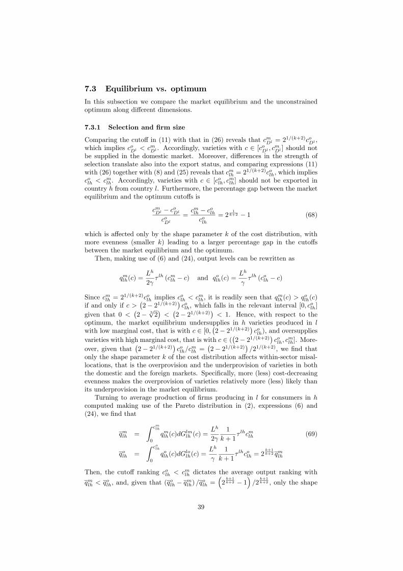
7.3 Equilibrium vs. optimum

In this subsection we compare the market equilibrium and the unconstrainedoptimum along different dimensions.

7.3.1 Selection and firm size

Comparing the cutoff in (11) with that in (26) reveals that cmDl = 21/(k+2)coDl ,which implies coDl < cmDl . Accordingly, varieties with c ∈ [coDl , c

mDl ] should not

be supplied in the domestic market. Moreover, differences in the strength ofselection translate also into the export status, and comparing expressions (11)with (26) together with (8) and (25) reveals that cmlh = 21/(k+2)colh, which impliescolh < cmlh. Accordingly, varieties with c ∈ [colh, c

mlh] should not be exported in

country h from country l. Furthermore, the percentage gap between the marketequilibrium and the optimum cutoffs is

cmDl − coDl

coDl

=cmlh − colhcolh

= 21

k+2 − 1 (68)

which is affected only by the shape parameter k of the cost distribution, withmore evenness (smaller k) leading to a larger percentage gap in the cutoffsbetween the market equilibrium and the optimum.

Then, making use of (6) and (24), output levels can be rewritten as

qmlh(c) =Lh

2γτ lh (cmlh − c) and qolh(c) =

Lh

γτ lh (colh − c)

Since cmlh = 21/(k+2)colh implies colh < cmlh, it is readily seen that q

mlh(c) > qolh(c)

if and only if c >(2− 21/(k+2)

)colh, which falls in the relevant interval [0, colh]

given that 0 <(2− 3√

2)<(2− 21/(k+2)

)< 1. Hence, with respect to the

optimum, the market equilibrium undersupplies in h varieties produced in lwith low marginal cost, that is with c ∈ [0,

(2− 21/(k+2)

)colh), and oversupplies

varieties with high marginal cost, that is with c ∈ ((2− 21/(k+2)

)colh, c

mlh]. More-

over, given that(2− 21/(k+2)

)colh/c

mlh =

(2− 21/(k+2)

)/21/(k+2), we find that

only the shape parameter k of the cost distribution affects within-sector misal-locations, that is the overprovision and the underprovision of varieties in boththe domestic and the foreign markets. Specifically, more (less) cost-decreasingevenness makes the overprovision of varieties relatively more (less) likely thanits underprovision in the market equilibrium.

Turning to average production of firms producing in l for consumers in hcomputed making use of the Pareto distribution in (2), expressions (6) and(24), we find that

qmlh =

∫ cmlh

0

qmlh(c)dGlmlh (c) =Lh

2γ

1

k + 1τ lhcmlh (69)

qolh =

∫ colh

0

qolh(c)dGlolh(c) =Lh

γ

1

k + 1τ lhcolh = 2

k+1k+2 qmlh

Then, the cutoff ranking colh < cmlh dictates the average output ranking with

qmlh < qolh, and, given that (qolh − qmlh) /qolh =(

2k+1k+2 − 1

)/2

k+1k+2 , only the shape

39

parameter k affects the percentage gap of the average quantities produced foreach country in the market and in the optimum case, with more (less) cost-decreasing evenness decreasing (increasing) the percentage gap in average firmsize between the market equilibrium and the optimum.The average quantity sold in h by domestic and foreign firms in the market

equilibrium, computed making use of (69) and (8), is

qmh =

M∑l=1

Nmlh q

mlh

M∑l=1

Nmlh

=Lh

2γ

1

k + 1τhhcmDh , (70)

and the average quantity of a variety available in h in the optimum case thatmaking use of (69), (25) and (70) is

qoh =

M∑l=1

Nolhq

olh

M∑l=1

Nolh

= 2k+1k+2 qmh , (71)

and it can be readily verified that qoh > qmh . The percentage gap between theaverage supply of a variety in a country in the market equilibrium and theoptimum is

qoh − qmhqoh

=2k+1k+2 − 1

2k+1k+2

=qolh − qmlhqolh

which is affected only by the shape parameter k of the cost distribution, withmore (less) evenness leading to a smaller (larger) percentage gap in the averagesupply of varieties in each country between the market equilibrium and theoptimum.

7.3.2 The total size of the differentiated sector

Then, making use of (70) and of Nmh from (16), the total quantities sold of the

differentiated varieties in h in the market evaluates to

Nmh q

mh =

Lh

η

(α− τhhcmDh

)(72)

that can be used to evaluate the effi ciency of the dimension of the differentiatedgoods sector (that is, the total supply of differentiated varieties) in the market foreach country h. Indeed, this can be compared with the corresponding dimensionof the differentiated good sector for the first best planner No

hqoh obtained making

use of (71), (67) and cmDl = 21/(k+2)coDl ,

Nohqoh =

Lh

η

(α− τhhcoDh

)(73)

Hence, coDh < cmDh implies Nohqoh > Nm

h qmh , and, therefore, in the market equilib-

rium the total supply of differentiated varieties is smaller than optimal in eachcountry. Using (72) and (73), we can write that

Nohqoh −Nm

h qmh

Nohqoh

=cmDh − coDh

coDh

τhhcoDh

α− τhhcoDh

40

In this expression, the percentage gap between the market equilibrium and theoptimum cutoffs (cmDh − coDh)/coDh is only affected by k, while larger values of

the market size Lh and smaller values of γ and ofM∑h=1

[fh(chM)k |Chl|] / |P |

(which is determined by the relative value of all f l(clM)kdefining the technol-

ogy available in all countries and trade barriers) lead to smaller coDh and, conse-quently, smaller τhhcoDh/

(α− τhhcoDh

). Accordingly, larger values of Lh and of

M∑h=1

[fh(chM)k |Chl|] / |P | imply smaller values for the ratio (No

hqoh −Nm

h qmh ) /No

hqoh,

while the impact of k is ambiguous.Finally, the comparison on product variety between No

h in (67) and Nmh in

(16), and the comparison on entry between N loE in (27) and N lm

E in (17), arepresented in the text of the paper.

8 Appendix B. The constrained planners in theopen economy

The second and the third best planners can not enforce marginal cost pricingby affecting the choices of each firm individually. However, the second bestplanner can affect firms choices controlling the cutoff and the number of firmsthat operate in the markets, while the third best planner can only control thenumber of firms that operate in the markets.Hence, the second best planner maximizes (23) with respect to cij and N i

E

∀i, j = 1, ....,M , while the third best planner maximizes the same expressiononly with respect to N i

E ∀i = 1, ....,M . Both maximizations are subject to: theprofit maximizing quantity qhl(c) in (36) and the selection conditions in (12). Inaddition, the third best planner has to consider the additional constraint givenby the free entry condition for each country l in (9).

In general, substituting quantities from (36) into (23) and making use of (2),allows to rewrite the problem of the constrained planner as the maximization of

W =

M∑l=1

U l(Ll) =

M∑l=1

ql0Ll +

M∑l=1

Ll −M∑l=1

f lN lE + (74)

−M∑l=1

N lE

1(clM)k M∑

h=1

[Lh

2γ

(τ lh)2 (

clh)k+2 k

(k + 2) (k + 1)

]+

+α

M∑l=1

Ll

2γ

M∑h=1

[τhlNh

E

1(chM)k (chl)k+1 1

(k + 1)

]+

−1

4

M∑l=1

Ll

γ

M∑h=1

[(τhl)2NhE

1(chM)k (chl)k+2 1

(k + 2) (k + 1)

]+

− η

8γ2

M∑l=1

Ll[M∑h=1

(τhlNh

E

1(chM)k (chl)k+1 1

(k + 1)

)]2

with respect to cij and N iE ∀i, j = 1, ....,M for the second best planner, and

with respect to N iE ∀i = 1, ....,M for the third best planner.

41

8.1 The second best planner

The first order condition for the maximization of (74) with respect to cij , ∂W∂cij =

0, is

−N iE

1(ciM)k Lj2γ

(τ ij)2 (

csij)k+1 k

(k + 1)+

+αLj

2γτ ijN i

E

1(ciM)k (csij)k +

−1

4

Lj

γ

(τ ij)2N iE

1(ciM)k (csij)k+1 1

(k + 1)+

− η

4γ2Lj

[M∑h=1

(τhjNh

E

1(chM)k (cshj)k+1 1

(k + 1)

)]τ ijN i

E

1(ciM)k (csij)k = 0

that can be simplified as follows

M∑h=1

(τhjNh

E

1(chM)k (cshj)k+1

)=

2γ (k + 1)

η

[α− 1

2

2k + 1

k + 1τ ijcsij

](75)

Given that previous expression holds also for i = j, and we can substitute jto i to have τ jjcsDj into the right hand side at the place of τ ijcsij , this impliesthat the relationship between the cutoffs of the two types of firms (domesticand foreign) selling in the same market has to be

csij =τ jj

τ ijcsDj ∀i, j = 1, ....,M

Making use of csij = τ jjcsDj/τ ij , expression (75) can be rewritten as follows

M∑h=1

(ρhjNh

E

1(chM)k)

=2γ (k + 1)

η

(α− 1

22k+1k+1 τ

jjcsDj

)(τ jjcsDj

)k+1

This gives a system of M linear equations that can be solved using Cramer’srule for the number of entrants in the M countries, with

N lsE =

2γ (k + 1)(clM)k M∑

h=1

(α− 1

22k+1k+1 τ

hhcsDh)(

τhhcsDh

)k+1 |Clh|

η |P | (76)

The first order condition for the maximization of (74) with respect to N iE ,

42

∂W∂Ni

E= 0, is

−f i − 1(ciM)k M∑

h=1

[Lh

2γ

(τ ih)2

(csih)k+2 k

(k + 2) (k + 1)

]+ (77)

+α

M∑l=1

[Ll

2γτ il

1(ciM)k (csil)

k+1 1

(k + 1)

]+

−1

4

M∑l=1

[Ll

γ

(τ il)2 1(

ciM)k (csil)

k+2 1

(k + 2) (k + 1)

]+

− η

4γ2

M∑l=1

Ll

[M∑h=1

(τhlNh

E

1(chM)k (cshl)

k+1 1

(k + 1)

)]τ il (csil)

k+1

(k + 1)(ciM)k

= 0

that making use of csij = τ jjcsDj/τ ij and (75) can be rewritten and simplified asfollows

M∑l=1

[Llρil

(τ llcsDl

)k+2]

=4γ (k + 2) (k + 1)

2 (ciM)kf i

2k + 1

This yields a system ofM equations that can be solved to find theM equilibriumdomestic cutoffs using Cramer’s rule:

csDl =1

τ ll

4γ (k + 2) (k + 1)

2

(2k + 1)Ll

M∑h=1

[fh(chM)k |Chl|]

|P |

1

k+2

(78)

8.2 The third best planner

The first order condition for the maximization of (74) with respect toN iE ,

∂W∂Ni

E=

0, for the third best planner corresponds to the first order condition with respectto N i

E for the second best planner given in expression (77) where csil is replaced

by cmil , that is the cutoff for the third best planner that correspond to that of themarket. Then substituting f i from (9), making use of the Pareto distribution in(2) and of the relationship between the cutoffs in (8), and simplifying becomes

M∑l=1

Llρil

(τ llcmDl

)k+1

[(τ llcmDl

)k+1M∑h=1

(ρhlNh

E

1(chM)k)− 2γ (k + 1)

η

(α− 1

2

2k + 3

k + 2τ llcmDl

)]= 0

Previous equation has a solution when, for all l, the expression in the squarebrackets is equal to zero, that is when

M∑h=1

(ρhlNh

E

1(chM)k)

=2γ (k + 1)

η

[α− 1

22k+3k+2

(τ llcmDl

)](τ llcm

Dl

)k+1

This gives a system of M linear equations that can be solved using Cramer’srule for the number of entrants in the M countries with

N ltE =

2γ (k + 1)(clM)k M∑

h=1

[(α− 1

22k+3k+2 τ

hhcmDh)(

τhhcmDh

)k+1 |Clh|]

η |P | (79)

43

9 C. Implementation of the constrained solu-tions in the open economy

Making use of (37), the average price set in l by firms producing in h is

phl =2k + 1

2 (k + 1)τhlchl − shl (80)

Hence, making use of (80) and (12), the average price of varieties sold in l is

pl =

M∑h=1

Nhlphl

M∑h=1

Nhl

=2k + 1

2 (k + 1)

M∑h=1

NhE

(chlchM

)kτhlchl

M∑h=1

NhE

(chlchM

)k −

M∑h=1

NhE

(chlchM

)kshl

M∑h=1

NhE

(chlchM

)k (81)

Then, given that for both the constrained planners hold sil = sjl = sl andcil = τ llcDl/τ il, pl in (81) can be rewritten as

pl =2k + 1

2 (k + 1)τ llcDl − sl (82)

Then, substituting chl = τ llcDl/τhl into (35) with shl = sl gives

plmax = τ llcDl − sl (83)

Substituting plmax from (83) and pl from (82) into the definition of plmax inthe zero cutoff profit condition (5) yields

Nl =2γ (k + 1)

η

(α− τ llcDl + sl

)τ llcDl

(84)

Finally, using (12), (13) and chl = τ llcDl/τhl gives

Nl =(τ llcDl

)k M∑h=1

ρhlNhE

(1

chM

)kthat can be used with (84) to find

M∑h=1

(ρhlNh

E

1(chM)k)

=2γ (k + 1)

η

(α− τ llcDl + sl

)(τ llcDl)

k+1

This gives a system of M linear equations that can be solved using Cramer’srule for the number of entrants in the M countries

N lE =

2γ (k + 1)(clM)k M∑

h=1

[(α−τhhcDh+sh)

(τhhcDh)k+1 |Clh|

]η |P | (85)

Notice that the expression for N lE in (85) is common for both the second and

the third best planner. However, the expressions for the cutoffs cDh and thesubsidies sh differ for the two planners.

44

9.1 The implementation of the second best solution

The solution N lE for the second best planner in (76) can be implemented setting

subsidies sh for all countries in such a way that the expression for N lE in (76)

and (85) are equal. This requires

M∑h=1

[(α− τhhcsDh + sh

)(τhhcs

Dh

)k+1|Clh|

]=

M∑h=1

(α− 1

22k+1k+1 τ

hhcsDh

)(τhhcs

Dh

)k+1|Clh|

for all l = 1, ...,M . This implies

M∑h=1

(sh − 1

2(k+1)τhhcsDh

)(τhhcs

Dh

)k+1|Clh|

= 0

which is satisfied when

sh =1

2 (k + 1)τhhcsDh ∀h = 1, ....,M

Then, the second best planner uses lump-sum entry taxes per entrant ineach country h,

(Th)s, to set the cutoffs. Specifically, the ‘free entry condition’

for firms producing in h can be stated as

M∑l=1

[∫ chl

0

Ll

4γ

(τhl)2

(chl − c)2dGh(c)

]= fh +

(Th)s

that making use of the Pareto distribution (2) and cshl = τ llcsDl/τhl can be

rewritten as

M∑l=1

[ρhlLl

(τ llcsDl

)k+2]

= 2γ(chM)k

(k + 2) (k + 1)[fh +

(Th)s]

This yields a system of M equations that can be solved using Cramer’s rule tofind the M equilibrium cutoffs

csDl =1

τ ll

2γ (k + 2) (k + 1)

Ll

M∑h=1

(chM)k [

fh +(Th)s] |Chl|

|P |

1

k+2

(86)

Specifically, the solutions csDl for the second best planner in (86) can be usedto set Th∀h = 1, ...,M to implement the solutions in (78). The two systemsgive the same solutions for the cutoff of country l if and only if the followingequation holds

M∑h=1

[(chM)k (

fh +(Th)s) |Chl|] =

2 (k + 1)

2k + 1

M∑h=1

[fh(chM)k |Chl|]

45

This must be true for all M countries (so there is an equation of this type forall l = 1, ....M) and it can be simplified as

M∑h=1

[(chM)k ((

Th)s − fh

2k + 1

)|Chl|

]= 0

which is satisfied when (Th)s

=fh

2k + 1∀h = 1, ....,M

9.2 The implementation of the third best solution

We recall that the cutoffs for the third best planner are those of the market.The solution N l

E for the third best planner in (79) can be implemented settingsubsidies

(sh)tfor all countries in such a way that the expression for N l

E in (79)and (85) are equal, which requires

M∑h=1

[α− τhhcmDh +

(sh)t](

τhhcmDh

)k+1|Clh|

=

M∑h=1

(α− 1

22k+3k+2 τ

hhcmDh

)(τhhcm

Dh

)k+1|Clh|

for all l = 1, ...,M . This implies

M∑h=1

[(sh)t − 1

2(k+2)τhhcmDh

](τhhcm

Dh

)k+1|Clh|

= 0

which is satisfied when(sh)t

=1

2 (k + 2)τhhcmDh ∀h = 1, ....,M

46