GEOGRAPHIC MAPS CLASSIFICATION BASED ON LAB COLOR SYSTEM

International Journal of Computer Networks & Communications (IJCNC) Vol.8, No.3, May 2016

DOI: 10.5121/ijcnc.2016.8306 81

GEOGRAPHIC MAPS CLASSIFICATION BASED ON

L*A*B COLOR SYSTEM

Salam m. Ghandour1 and Nidal M. Turab

2

1CIS Dept. University Of Jordan, Amman Jordan

2Computer Networks And Information Security Dept. , Al Ahliyya Amman University,

Amman- Jordan

ABSTRACT

Today any geographic information system (GIS) layers became vital part of any GIS system , and

consequently , the need for developing automatic approaches to extract GIS layers from different image

maps like digital maps or satellite images is very important.

Map classification can be defined as an image processing technique which creates thematic maps from

scanned paper maps or remotely sensed images. Each resultant theme will represent a GIS layer of the

images.

A new proposed approach to extract GIS layers (classes) automatically based on L*A*B colorsystem

selected from ( A and B ) is proposed in this paper, our experiments shows that the hsi color space gives

better than L*A*B.

KEYWORDS

L*a*b color space, HSI color space, GIS, GIS layers, classification

1. INTRODUCTION

Map classification techniques used to extract layers had been published and studies recently.

Classification techniques are classified into: [9].

• Supervised classification: the researcher or user performs the following steps:

• The interesting geographic region to test assumption is specified.

• Carefully classifies the classes of interest.

• Selects asuitableclassification algorithm and then collects initial data used to train

the algorithm.

• Selects the characteristicsof the most optimal variables.

• Applies classification algorithm produces to produce map and assigns an

unknown pixel to its dominant class.

• Evaluates any errors.

• Unsupervised classification techniques: the researcher or user performs the following

steps:

• Identifies how many classes to generate and which bands to use.

• The software clusters the pixels into the set of classes.

• Identifies the classes.


82

In this paper, we contribute the L*a*b color space model to extract GIS layers. This is performed

by selecting the a* and b* components of the L*a*b color space model. We then compare our

results with HIS color model [1].

The paper is organized as follows. In section 1 is an introduction to classification techniques;

related work is summarized in section 2. Our proposed new algorithm for automatic extraction of

GIS Layers is explained in section 3. While in section 4 we summarize the results of the

experiments that conducted to evaluate the proposed map clustering system. Finally, the paper is

concluded in section 5.

2. RELATED WORK

The maximum likelihood algorithm is one of the familiar supervised classification algorithms

[8],[10]. The maximum likelihood decision rule is based on calculating the probability of pixels

belonging to a predefined set of classes, thenthesepixelsare assigned to the highest probability

class. However, this algorithm assumes normally distribution of training data as shown in [5]..

The authors of [3] presented an unsupervised clustering, where the image map data is split,the

resulting classification mapis composedof a set of classes. Then theresulting classes are assigned

to layers. In [4] the authors studied the integrated spectral information with measures of texture,

in the form of the variance and the variogram;theyfound that the accuracy was greater than of

maximum likelihood. I n [6] the authors presented an overview of significant advances made in

the emerging field of nature-inspired computing (NIC); with a focus on the physics- and biology-

based approaches and algorithms. They concluded that the field of nature-inspired computing is

large and expanding.

In [10] the authors proposed an Agglomerative Hierarchical Clustering based on High-Resolution

Remote Sensing Image Segmentation Algorithm.Their conducted experiment shows that the

results of this algorithm are better than the K-Means’ and are very close to the artificial extraction

results.

3. PROPOSED APPROACH

Our proposed approach for GEOGRAPHIC MAPS CLASSIFICATION BASED ON L*a*b

COLOR SYSTEM. . The L*a*b color space is a geometrical color-opponent space which has the

shape of a sphere. Its composed of the following ingredients: L is the lightness, while a and b

together represent the color and saturation information [7], [11]. Figure 1 illustrates the L*a*b

color space.

The L, a, and b axes provide a practical combination of the orthogonal simplicity of the RGB

color space and the other color spaces such as HSI which are used in many color management

systems[11].

The L*a*b color space is considered to be “perceptually uniform,” which means that any

detectable visual difference in the color space can be represented by a constant distance in any

direction or location. L*a*b is used widely as a standard space to compare colors [2], [11]. In this

paper, we are interested in the ( a , b ) component only.


83

Figure 1. L*a*b color space [2]

Equation (1) represents a mathematical relationship between L, a, b and R, G, B [11]:

�� = � 13 13 13−√26 −√26 2√261√2

−1√2 0 ��

��∗ ��

Equation1. The relationship between L, a, b and R, G, B

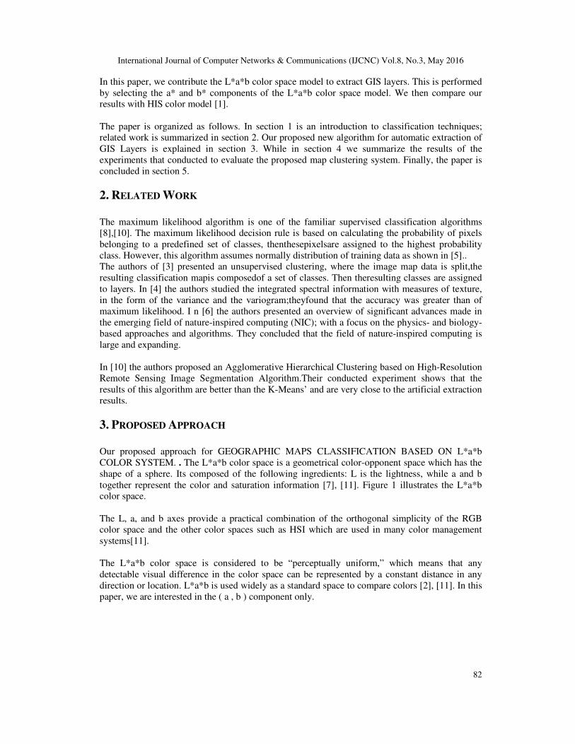
The proposed map clustering system uses image processing and machine learning techniques.

Figure 2 illustrates the flowchart for the proposed system. The first stage after the system start up

is to select the input map image. Then, that image is processed for contrast enhancement as a pre-

processing stage. At this stage, the image color values distribution is changed to cover a wider

range of colors.


84

Figure 2. Flowchart of the proposed map clustering system

The enhancement of image contrast yields better clustering results when the clustering is based on

colors. Figure 3 shows an example for image contrast enhancement.

Figure 3. An example of contrast enhancement

Then, the color space used for representing the image is converted to another color space that

allowsthe separation of the color components and the light intensity unlike the original RGB color

space. This research investigated two color spaces: HSI and L*a*b.

Figure 4 gives an example of the L*a*b components for an image. The HSI color space gives

better clustering results than L*a*b, as will be discussed in detail later.


Figure 4.

The system then extracts the color components from the converted image representation and

ignores the lightness component.

Finally, the system sensitivity level should be specified by the user so that the system can define

the sensitivity regions. Sensitivity level is an integer number that starts from 1 and up to image bit

depth (color depth).

The sensitivity level is used to define the number of equally

HSI or L*a*b chromaticity distribution, which are called sensi

chromaticity distribution in HSI color space, a slice of the HSI color space is taken at a fixed

intensity value. The same is done in the L*a*b color space, where a chromaticity distribution is

taken at a fixed lightness. Figure 5 shows the chromaticity distribution taken from each color

space.

Figure 5.The chromaticity distribution for: ( a,b) L*a*b and HIS

A sensitivity region is in the chromaticity distribution which contains colors to be considered as a

cluster. The number of the regions is defined by the equation (2):

Number of sensitivity regions = 2


Figure 4.The L*a*b components for an image


ignores the lightness component.


ivity level is an integer number that starts from 1 and up to image bit

The sensitivity level is used to define the number of equally-sized color regions obtained from the

HSI or L*a*b chromaticity distribution, which are called sensitivity regions. To define the



re 5 shows the chromaticity distribution taken from each color

chromaticity distribution for: ( a,b) L*a*b and HIS


umber of the regions is defined by the equation (2):

Number of sensitivity regions = 21+sensitivity level


85



ivity level is an integer number that starts from 1 and up to image bit

sized color regions obtained from the

tivity regions. To define the



re 5 shows the chromaticity distribution taken from each color



86

Figure 6 shows an example of sensitivity regions for L*a*b color space when the sensitivity level

is 3 and it contains 16 sensitivity regions.

Figure 6.An example of sensitivity regions for L*a*b color space when the sensitivity level is 3

For each sensitivity region, all the colors in that region are used in a mask to extract the pixels

having matching colors from the input map image and the pixels having other colors will be

masked as black pixels. After all sensitivity regions are used in the masks, the system will have a

number of clusters equal to the number of sensitivity regions. Figure 7 shows the output of

masking a sample image with one sensitivity region.

Figure .7 the output of masking a sample image with one sensitivity region

For each sensitivity level selection, a threshold is also selected for the acceptable area ratio for the

clusters to ensure excluding the negligible clusters as a post-processing stage. This is important to

only have clusters that actually represent something meaningful. When the sensitivity level is

small, the threshold for the acceptable area ratio can have higher values than the threshold used

when the sensitivity level is high because the number of colors included in small sensitivity

regions is small, and therefore it is more likely to have small clusters which cannot be ignored.

Figure 8 illustrates the cluster area ratios for eight clusters that represent the full area of an image

including the negligible clusters. The clusters having an area ratio less than 5% were neglected.


87

Figure 8.The cluster area ratios for eight clusters that represent the full area of an image including the

negligible clusters

Figure 9 shows an example of the image resulting from the system after it finishes processing the

input map image with the steps discussed above. The Sensitivity level used in the example is 1,

yielding 4 sensitivity regions. There was 1 negligible cluster when using a threshold for the

acceptable cluster area ratio 10% with HSI color space.

Figure 9. An example of map image clustering processed in the proposed system

4. RESULTS ANALYSIS

This part summarizes the experiments performed to evaluate the proposed map clustering system.

The experiments investigate using two color spaces: HSI and L*a*b.

4.1 QUALITATIVE EXPERIMENTS

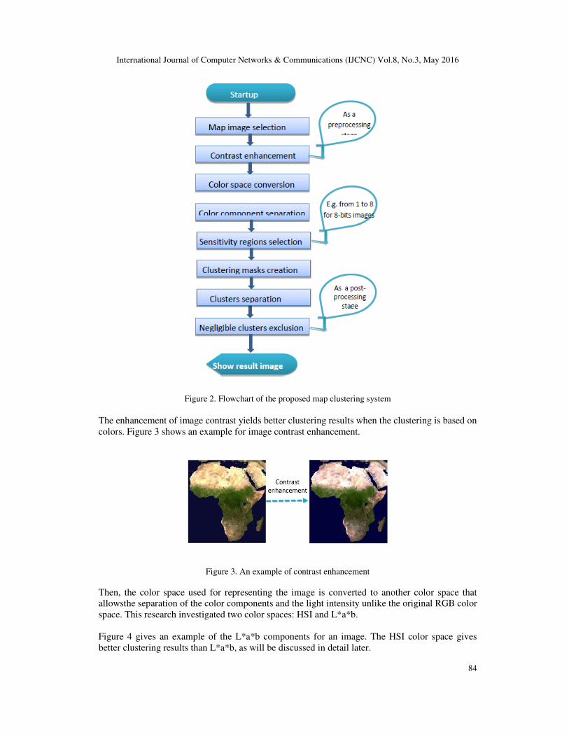
The qualitative evaluation performed in this research shows that the clustering results when using

HIS color space is better than the results when using L*a*b color space, as shown in Figure10.


Figure 10. Map image clustering results when using HSI and L*a*b color spaces

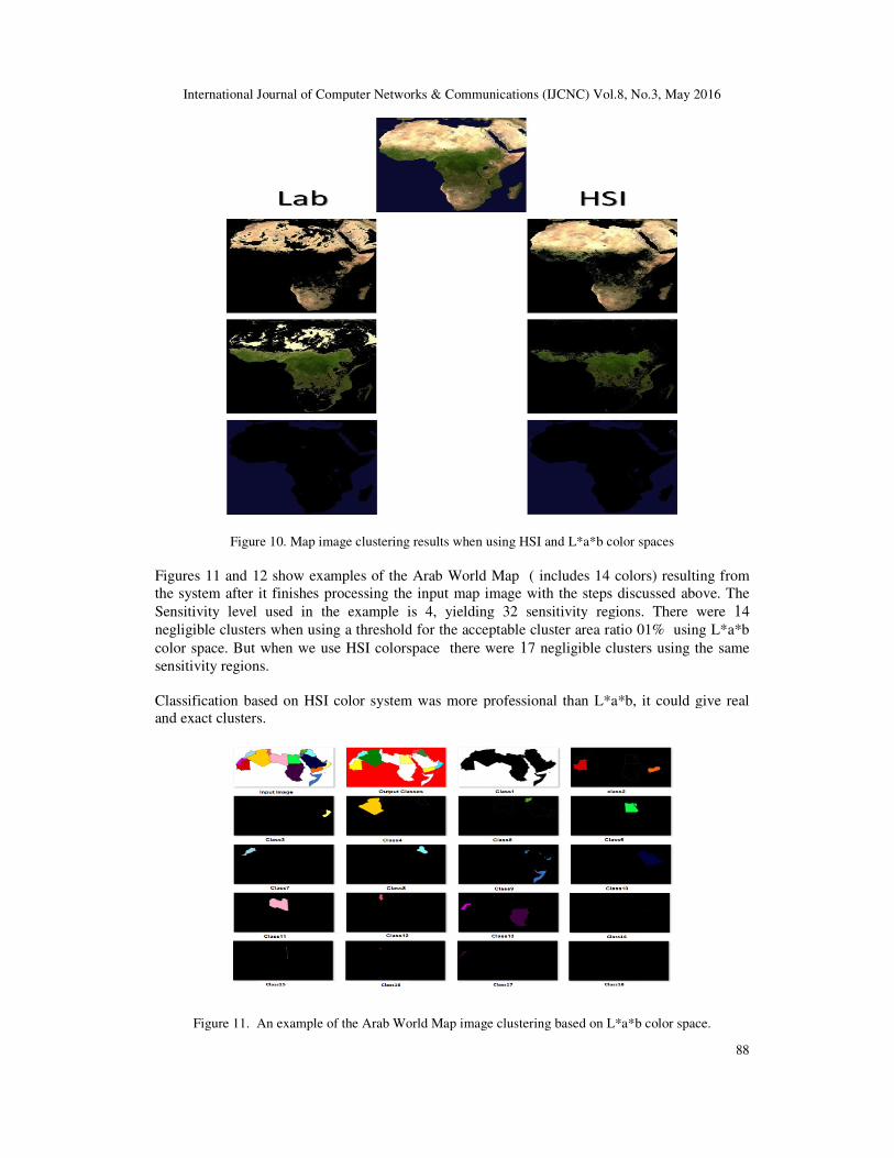
Figures 11 and 12 show examples of the Arab World Map ( includes 14 colors) resulting from

the system after it finishes processing the input map image with the steps discussed above. The

Sensitivity level used in the example is 4, yielding 32 sensitivity

negligible clusters when using a threshold for the acceptable cluster area ratio 01% using L*a*b

color space. But when we use HSI colorspace there were

sensitivity regions.

Classification based on HSI color system was more professional than L*a*b, it could give real

and exact clusters.

Figure 11. An example of the Arab World Map image





Sensitivity level used in the example is 4, yielding 32 sensitivity regions. There were


color space. But when we use HSI colorspace there were 17 negligible clusters using the same

d on HSI color system was more professional than L*a*b, it could give real

Figure 11. An example of the Arab World Map image clustering based on L*a*b color space.


88




regions. There were 14


7 negligible clusters using the same

d on HSI color system was more professional than L*a*b, it could give real

on L*a*b color space.


Figure 12. An example of the Arab World Map image

4.2 QUANTITATIVE EXPERIMENTS

As previously discussed, the sensitivity level used in the system controls the number of clusters

found in the image, based on Equation (2). Figure 13 shows the number of clusters in HSI and

L*a*b color spaces with different negligible area ratios (NR).

Figure 13. The number of clusters in HSI and L*a*b color spaces with different negligible area ratios (This

graph indicates that the numbers of clusters when it was little)

The Figure shows that when the sensitivity level is increased, the number of clusters in HSI color

space is increasing reasonably even though a negligible area ratio is used. However, after

sensitivity level 3 (when using L*a*b color space), the number of clusters decreases unexpec

- it was expected to increase as what happens when the HSI color space is used. This huge

unexpected decrease in the number of clusters is the result of dividing the image to meaningless

clusters whereas the visuallysimilar regions on the map are d

of one cluster and consequently, instead of one acceptable cluster, the area of one region will be

divided to many clusters of which many are negligible.

Figure 14 shows that when the sensitivity level is increased,

space will increase. However, the increase in the number of clusters in L*a*b in sensitivity levels

3 - 4 was arbitrary and inaccurate .


Figure 12. An example of the Arab World Map image clustering based on HSI color space

XPERIMENTS



spaces with different negligible area ratios (NR).


graph indicates that the numbers of clusters when it was little)

the sensitivity level is increased, the number of clusters in HSI color


sensitivity level 3 (when using L*a*b color space), the number of clusters decreases unexpec

it was expected to increase as what happens when the HSI color space is used. This huge


clusters whereas the visuallysimilar regions on the map are divided into multiple clusters instead


divided to many clusters of which many are negligible.

Figure 14 shows that when the sensitivity level is increased, the number of clusters in HSI color


4 was arbitrary and inaccurate .


89

on HSI color space




the sensitivity level is increased, the number of clusters in HSI color


sensitivity level 3 (when using L*a*b color space), the number of clusters decreases unexpectedly

it was expected to increase as what happens when the HSI color space is used. This huge


ivided into multiple clusters instead


the number of clusters in HSI color



Figure 14. The number of clusters in HSI and L*a*b color spaces with differe

graph indicates The numbers of clusters when it was 14)

The performance of the system when using HSI and L*a*b color spaces was also investigated.

For this experiment, the time required to process an image of size 6.5 Mega

using the function timeit available on Mathworks. Time measurements have been performed in

the following specifications:

• Windows 7 64-bit

• Intel(R) Core(TM) i7-2670QM CPU @ 2.20GHz

• 6M Cache

• 6144MB RAM

• MATLAB R2013a software package

Figure 15 shows the time required to complete the map image clustering in the proposed system

when using HSI and L*a*b color spaces.

Figure 15.the time required to complete the map image clustering in the proposed system when using HSI

The time required increases when the sensitivity level (SL) is increased because the number of

masks used in clustering increases when the number of sensitivity regions increase, which means

more processing is required. The difference in performance betwee

and when using L*a*b color spaces is small, with a mean difference equals to two seconds. The

HSI color conversion is two seconds faster than L*a*b color conversion.



graph indicates The numbers of clusters when it was 14)


For this experiment, the time required to process an image of size 6.5 Mega-pixel is measured


2670QM CPU @ 2.20GHz

MATLAB R2013a software package

ure 15 shows the time required to complete the map image clustering in the proposed system

when using HSI and L*a*b color spaces.


and L*a*b color spaces.



more processing is required. The difference in performance between the system when using HSI


HSI color conversion is two seconds faster than L*a*b color conversion.


90

nt negligible area ratios (This


pixel is measured


ure 15 shows the time required to complete the map image clustering in the proposed system




n the system when using HSI



91

5. CONCLUSION

This paper presented an effective maps clustering system, in which a map image is processed to

categorize the natural regions in the map image into clusters, based on color. The system was

implemented using a combination of several image processing techniques, such as image contrast

enhancement, color space conversion and masking. The processed map image undergoes several

stages to extract the clusters, including a preprocessing stage which makes the clustering process

more accurate. Another addition proposed in the system to make it more effective, is sensitivity

level which will be used in the system to define the number of equally-sized color regions for

each cluster. Each region includes a set of color shades that will be mapped to a single cluster.

The presented research investigated the map images clustering system, evaluated the performance

and compared the efficiency of using two color spaces: HSI and L*a*b, using qualitative and

quantitative experiments. The results of the qualitative experiments performed showed that the

map image clustering results were better when using HSI than the when using L*a*b color space,

as the clusters were more accurate.

In quantitative experiments, using HSI color space was found to have an increase in the number

of clusters when increasing the sensitivity level. In other words, using HSI color space is more

effective in maps clustering when high sensitivity is required, whereas using L*a*b color space

yields many negligible clusters.

The time required to complete the map image clustering when using HSI and L*a*b color system

when changing the sensitivity level was also compared. The time required increases when

increasing sensitivity level. The required processing time when using HSI is smaller than when

using L*a*b color space.

To sum up, this research presented an effective map clustering system using image processing

techniques. The system achieves accurate clustering when using HSI color space with a slightly

better performance in the processing time needed.

6. FUTURE WORK

In addition to the research of the future, we aspire to the classification of geographical maps on

other color systems and to comparing the results of this research in order to produce the best

color classification model.

REFERENCES

[1] Al- ZoubiMoh'dBelal( 2010 ), A New Algorithm for Automatic Extraction of GIS Layers “,7th

International Multi-Conference on Systems Signals and Devices (SSD), IEEE, Amman.

[2] Arum .S Sari and Suciati .N ( 2014 ), Flower Classification using Combined a* b* Color and Fractal-

based Texture Feature “,Vol.7, No.2 , pp.357-368 , Surabaya, Indonesia : International Journal of

Hybrid Information Technology.

[3] Atkinsona .P.M, Lewisb .P, (2000), Geostatistical Classification for Remote Sensing: An

Introduction”, Computers &Geosciences vol. 26 , pp. 361-371.

[4] Berberoglua .S, Lloydb .C.D, Atkinsonb .P.M and Curranb .P.J, (2000), The Integration of Spectral

and Textural Information Using Neural Networks for Land Cover Mapping in The Mediterranean,

Computers & Geosciences, vol. 26, pp. 385-396.

[5] Caprioli .M, and Tarantino .E, (2001), Accuracy Assessment of Per-Field Classification Integrating

Very Fine SpatialResolution Satellite Imagery with Topographic Data, Journal of Geospatial

Engineering, vol. 3, no. 2, pp. 127-134.


92

[6] Farah .Y. A, Baki R. M, Yassin .A, Tahir.N and Ishak .W, (2009), Monitoring of Watermelon

Ripeness Based on Fuzzy Logic, WRI World Congress on Computer Science and Information

Engineering, pp.,67-70.

[7] Lei Xu (2011), A new method for license plate detection based on color and edge information of lab

space. In: Proceedings of International Conference on Multimedia and Signal Processing,

(CMSP’2011), p. 99- 102, USA: IEEE.

[8] Mena .J .B, (2003), State of the Art on Automatic Road Extraction for GIS Update: A Novel

Classification, Pattern Recognition Letters, vol. 24, no. 16, pp. 3037–3058.

[9] Mena .J .B, Malpica .J .A, (2005), An Automatic Method For Road Extraction in Rural and Semi-

Urban Areas Starting from High Resolution Satellite Imagery, Pattern Recognition Letters, vol. 26,

pp. 1201–1220,.

[10] Rongjie Liu, Zhang Jie, Song Pingjian, Shao Fengjing and Guanfeng Liu, (2008), An Agglomerative

Hierarchical Clustering Based High-Resolution Remote Sensing Image Segmentation Algorithm,

International Conference on Computer Science and Software Engineering, pp. 403-406.

[11] Russ .J.C ( 2011), The Image Processing Handbook, ISBN 9781439840450, US : CRC Press.

AUTHORS

Salam M. Gandour, received a BSc degree in software engineering from the ISRA University Amman,

Jordan, 2009 and an MSc in CIS from the University of Jordan, Amman in 2015. Her research interests

include Geographic Maps eLearning and IoT.

Dr.Nidal Mahmmoud Mustafa Turab received a BSc degree in communication engineering from the

University of Garounis, Benghazi, libya 1992 and an MSc in telecommunication engineering from the

University of Jordan, Amman in 1996. His PhD in computer science is from the Polytechnic University of

Bucharest, 2008. His research interests include WLAN security, computer network security and cloud

computing security, eLearning and Artificial Intelligent. He is an associate professor at Alhliyya

AmmanUniversity, Amman, Jordan

GEOGRAPHIC MAPS CLASSIFICATION BASED ON LAB COLOR SYSTEM

Education

Transcript of GEOGRAPHIC MAPS CLASSIFICATION BASED ON LAB COLOR SYSTEM

GEOGRAPHIC MAPS CLASSIFICATION BASED ON L*A*B COLOR SYSTEM

Education

Transcript of GEOGRAPHIC MAPS CLASSIFICATION BASED ON L*A*B COLOR SYSTEM

GEOGRAPHIC MAPS CLASSIFICATION BASED ON LAB COLOR SYSTEM

Transcript of GEOGRAPHIC MAPS CLASSIFICATION BASED ON LAB COLOR SYSTEM