1

Geography 245 - Geographic Information Systems

Vector Analysis in ArcGIS Tutorial

The objectives of this tutorial include:

1. Selecting features by location (spatial joins / location queries)

2. Analyzing vector data (buffering and overlaying)

3. Cleaning up or preparing vector data for analysis (clipping and dissolving)

Before beginning the tutorial, please map the \\geogsv01\classspace\G245S10\LabData

and \\geogsv01\classspace\G245S10\L245a or L245b\yourname server folders. The LabData folder

contains a folder called Eight. In it, you will find an archive called Lab8.zip that contains the data that

are needed for this tutorial and exercise 8. COPY the Lab8 archive to your server folder and unpack it.

1. Spatial joins: Learning how to connect polygons to lines

Often times it is useful to join attribute information from a polygon map to a line map. We performed

a similar operation in Lab6 when we joined polygons to points for the Colgate land cover assessment

exercise. In this case, let’s say we want to determine the total number of people that live in counties

that border each of the Interstate Highways in the United States.

• Launch ArcMap and open a new empty map. Add the US Counties and Roads_RT layers from

the C:\ESRI\ESRIDATA\USA folder. Place the roads on top of the counties so that you can

see both.

• Before proceeding any further make sure you change the projection of your dataframe to North

American Albers Equal Area Projection.

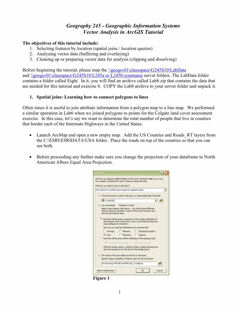
Figure 1

2

• Right click on the Roads_RT layer and select ‘Joins and Relates’ -> ‘Join’. In the window that

appears you select “Join data from another layer based on spatial location’. In this dialogue

box you can select the kind of spatial join you want to perform. Since we are interested in

knowing the total number of people in each county that each road intersects you should select

the first join option and ‘sum’.

• Provide a name and location of the new shapefile that this tool with create. Once your window

looks similar to Fig 1 above click ‘ok’ to run the command.

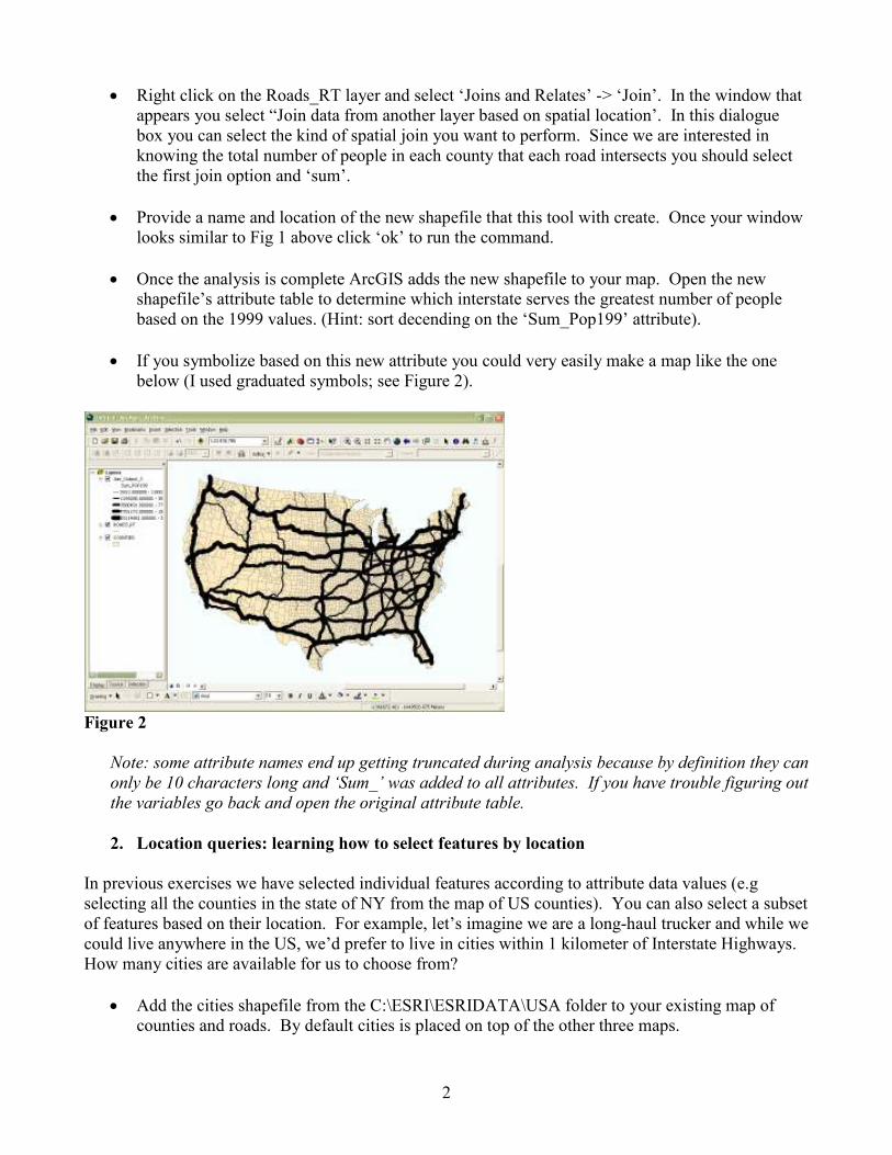
• Once the analysis is complete ArcGIS adds the new shapefile to your map. Open the new

shapefile’s attribute table to determine which interstate serves the greatest number of people

based on the 1999 values. (Hint: sort decending on the ‘Sum_Pop199’ attribute).

• If you symbolize based on this new attribute you could very easily make a map like the one

below (I used graduated symbols; see Figure 2).

Figure 2

Note: some attribute names end up getting truncated during analysis because by definition they can

only be 10 characters long and ‘Sum_’ was added to all attributes. If you have trouble figuring out

the variables go back and open the original attribute table.

2. Location queries: learning how to select features by location

In previous exercises we have selected individual features according to attribute data values (e.g

selecting all the counties in the state of NY from the map of US counties). You can also select a subset

of features based on their location. For example, let’s imagine we are a long-haul trucker and while we

could live anywhere in the US, we’d prefer to live in cities within 1 kilometer of Interstate Highways.

How many cities are available for us to choose from?

• Add the cities shapefile from the C:\ESRI\ESRIDATA\USA folder to your existing map of

counties and roads. By default cities is placed on top of the other three maps.

3

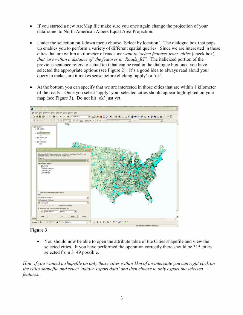
• If you started a new ArcMap file make sure you once again change the projection of your

dataframe to North American Albers Equal Area Projection.

• Under the selection pull-down menu choose ‘Select by location’. The dialogue box that pops

up enables you to perform a variety of different spatial queries. Since we are interested in those

cities that are within a kilometer of roads we want to ‘select features from’ cities (check box)

that ‘are within a distance of’ the features in ‘Roads_RT’. The italicized portion of the

previous sentence refers to actual text that can be read in the dialogue box once you have

selected the appropriate options (see Figure 2). It’s a good idea to always read aloud your

query to make sure it makes sense before clicking ‘apply’ or ‘ok’.

• At the bottom you can specify that we are interested in those cities that are within 1 kilometer

of the roads. Once you select ‘apply’ your selected cities should appear highlighted on your

map (see Figure 3). Do not hit ‘ok’ just yet.

Figure 3

• You should now be able to open the attribute table of the Cities shapefile and view the

selected cities. If you have performed the operation correctly there should be 315 cities

selected from 3149 possible.

Hint: if you wanted a shapefile on only those cities within 1km of an interstate you can right click on

the cities shapefile and select ‘data-> export data’ and then choose to only export the selected

features.

4

Let’s further imagine that after visiting these cities you decide that you want to live within 50 kms of a

lake. How many of the 316 cities are within 50kms of a lake?

• Add the lakes shapefile from the C:\ESRI\ESRIDATA\USA folder to your existing map of

counties and roads. By default lakes is placed on top of the other polygon maps.

• In the “I want to” pulldown menu at the top of the ‘Select By Location’ dialogue box

indicate that you want to ‘select from the currently selected features in’ option. This will

enable you to select from the 316 cities that are within 1 km of an interstate.

• This time you ‘want to select from the currently selected features in cities that are within a

distance of the features in lakes.’ Once again select the option to buffer, but this time

choose lakes and 50km. Your window should look like figure 4 below.

Figure 4

• You should find that 42 of the cities are both within 1 km of an interstate and 50 km of a lake.

3. Analyzing vector data (buffering and overlaying)

Each of the routines described above in part three are ultimately designed to select a unique subset of

objects from different map layers. However, suppose we want to analyze spatial data layers in a way

that creates entirely new objects. For example, rather than wanting to know how many cities are

within one kilometer of an interstate (selecting a unique subset of cities) we want to know what land

areas in the US are within a kilometer of an interstate? These land areas do not exist yet. They need to

be created from existing data. These kinds of questions require a different set of tools.

5

Let’s imagine that we want to determine all those areas in the US that are not within 50 kilometers of

an interstate, but are within 25 km of a river? We can do this by “buffering” the interstates at 50km

and overlaying the area outside the buffer with the area inside a 25km buffer of streams.

• Start a new ArcMap document (.mxd file) and add the Rivers, Roads_RT, and States layers

from the ESRI map files.

• Before proceeding any further make sure you change the projection of your dataframe to North

American Albers Equal Area Projection.

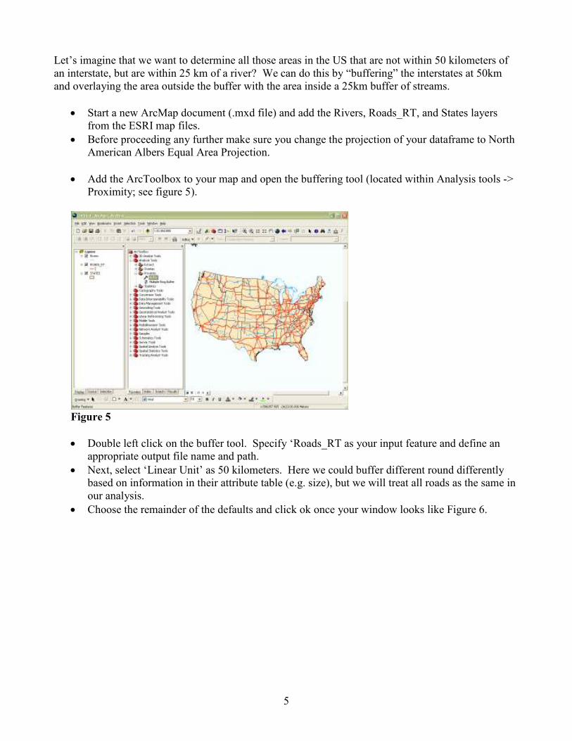
• Add the ArcToolbox to your map and open the buffering tool (located within Analysis tools ->

Proximity; see figure 5).

Figure 5

• Double left click on the buffer tool. Specify ‘Roads_RT as your input feature and define an

appropriate output file name and path.

• Next, select ‘Linear Unit’ as 50 kilometers. Here we could buffer different round differently

based on information in their attribute table (e.g. size), but we will treat all roads as the same in

our analysis.

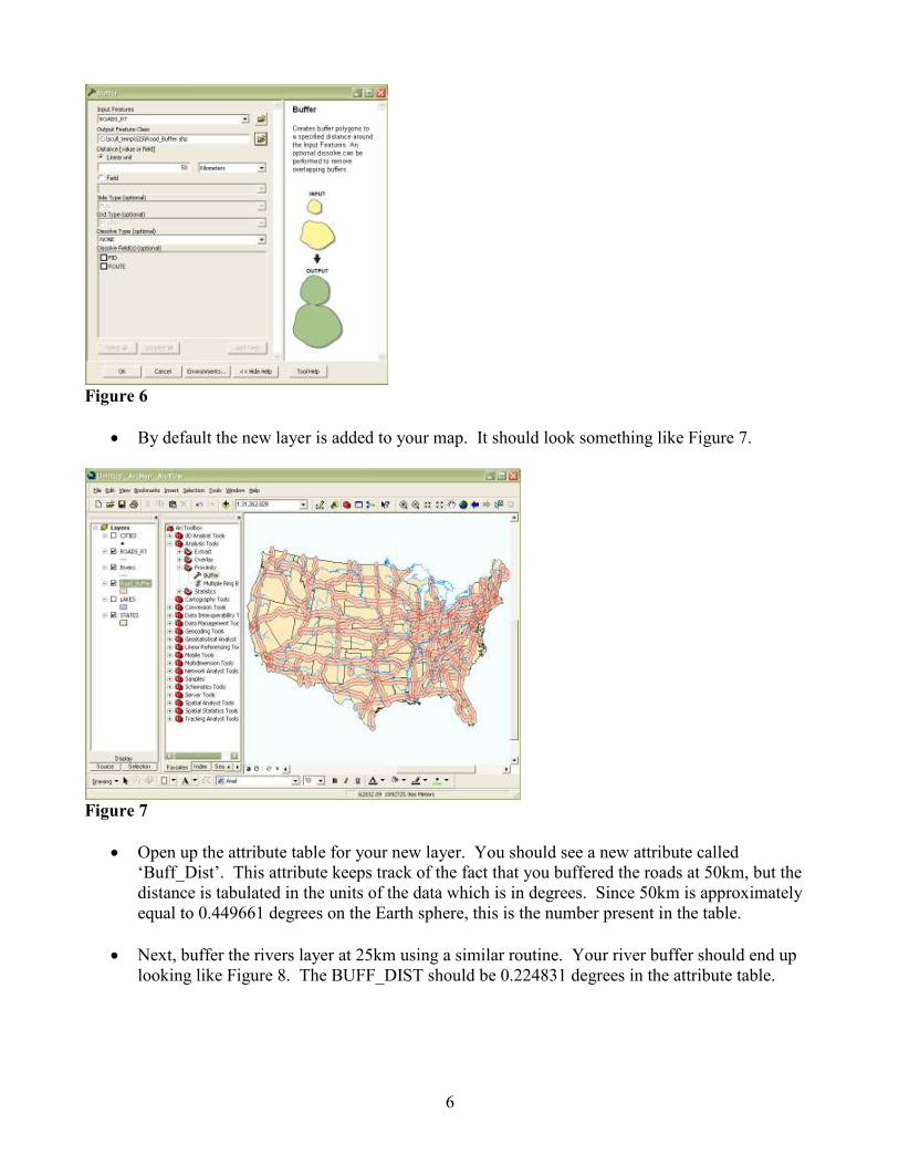
• Choose the remainder of the defaults and click ok once your window looks like Figure 6.

6

Figure 6

• By default the new layer is added to your map. It should look something like Figure 7.

Figure 7

• Open up the attribute table for your new layer. You should see a new attribute called

‘Buff_Dist’. This attribute keeps track of the fact that you buffered the roads at 50km, but the

distance is tabulated in the units of the data which is in degrees. Since 50km is approximately

equal to 0.449661 degrees on the Earth sphere, this is the number present in the table.

• Next, buffer the rivers layer at 25km using a similar routine. Your river buffer should end up

looking like Figure 8. The BUFF_DIST should be 0.224831 degrees in the attribute table.

7

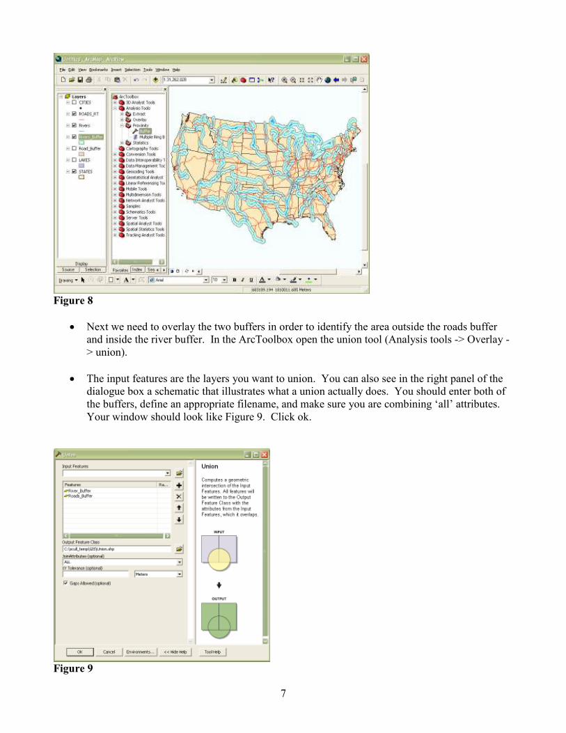
Figure 8

• Next we need to overlay the two buffers in order to identify the area outside the roads buffer

and inside the river buffer. In the ArcToolbox open the union tool (Analysis tools -> Overlay -

> union).

• The input features are the layers you want to union. You can also see in the right panel of the

dialogue box a schematic that illustrates what a union actually does. You should enter both of

the buffers, define an appropriate filename, and make sure you are combining ‘all’ attributes.

Your window should look like Figure 9. Click ok.

Figure 9

8

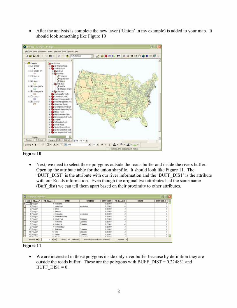
• After the analysis is complete the new layer (‘Union’ in my example) is added to your map. It

should look something like Figure 10

Figure 10

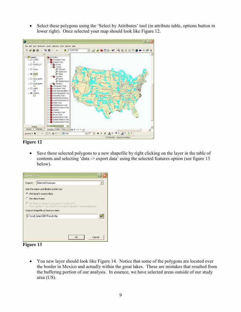
• Next, we need to select those polygons outside the roads buffer and inside the rivers buffer.

Open up the attribute table for the union shapfile. It should look like Figure 11. The

‘BUFF_DIST’ is the attribute with our river information and the ‘BUFF_DIS1’ is the attribute

with our Roads information. Even though the original two attributes had the same name

(Buff_dist) we can tell them apart based on their proximity to other attributes.

Figure 11

• We are interested in those polygons inside only river buffer because by definition they are

outside the roads buffer. These are the polygons with BUFF_DIST = 0.224831 and

BUFF_DIS1 = 0.

9

• Select these polygons using the ‘Select by Attributes’ tool (in attribute table, options button in

lower right). Once selected your map should look like Figure 12.

Figure 12

• Save these selected polygons to a new shapefile by right clicking on the layer in the table of

contents and selecting ‘data -> export data’ using the selected features option (see figure 13

below).

Figure 13

• You new layer should look like Figure 14. Notice that some of the polygons are located over

the border in Mexico and actually within the great lakes. These are mistakes that resulted from

the buffering portion of our analysis. In essence, we have selected areas outside of our study

area (US).

10

Figure 14

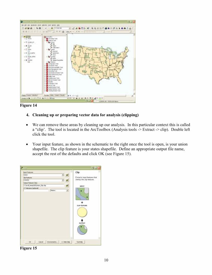
4. Cleaning up or preparing vector data for analysis (clipping)

• We can remove these areas by cleaning up our analysis. In this particular context this is called

a “clip’. The tool is located in the ArcToolbox (Analysis tools -> Extract -> clip). Double left

click the tool.

• Your input feature, as shown in the schematic to the right once the tool is open, is your union

shapefile. The clip feature is your states shapefile. Define an appropriate output file name,

accept the rest of the defaults and click OK (see Figure 15).

Figure 15

11

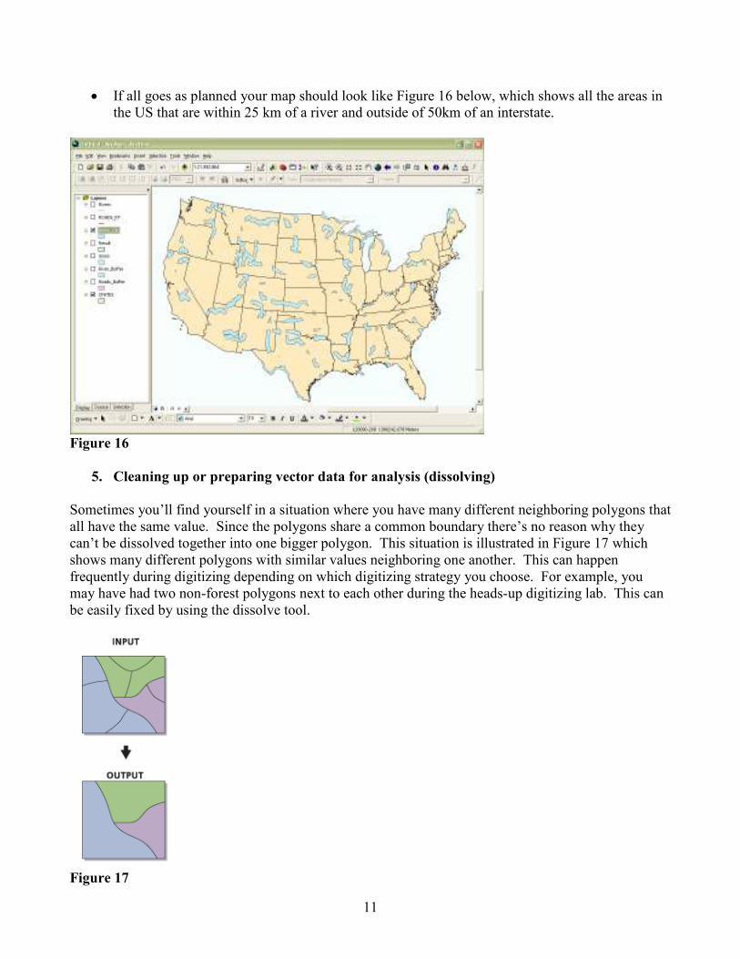
• If all goes as planned your map should look like Figure 16 below, which shows all the areas in

the US that are within 25 km of a river and outside of 50km of an interstate.

Figure 16

5. Cleaning up or preparing vector data for analysis (dissolving)

Sometimes you’ll find yourself in a situation where you have many different neighboring polygons that

all have the same value. Since the polygons share a common boundary there’s no reason why they

can’t be dissolved together into one bigger polygon. This situation is illustrated in Figure 17 which

shows many different polygons with similar values neighboring one another. This can happen

frequently during digitizing depending on which digitizing strategy you choose. For example, you

may have had two non-forest polygons next to each other during the heads-up digitizing lab. This can

be easily fixed by using the dissolve tool.

Figure 17

12

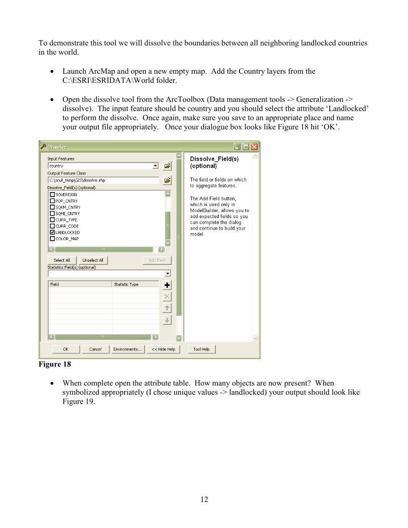
To demonstrate this tool we will dissolve the boundaries between all neighboring landlocked countries

in the world.

• Launch ArcMap and open a new empty map. Add the Country layers from the

C:\ESRI\ESRIDATA\World folder.

• Open the dissolve tool from the ArcToolbox (Data management tools -> Generalization ->

dissolve). The input feature should be country and you should select the attribute ‘Landlocked’

to perform the dissolve. Once again, make sure you save to an appropriate place and name

your output file appropriately. Once your dialogue box looks like Figure 18 hit ‘OK’.

Figure 18

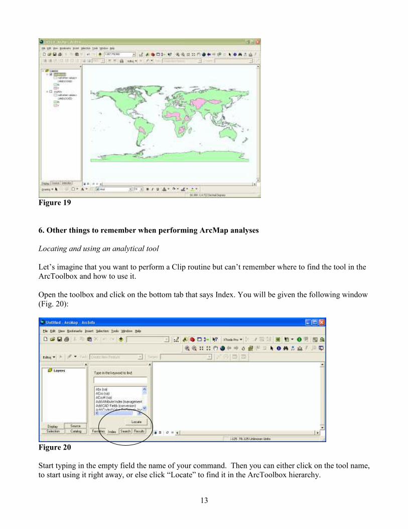
• When complete open the attribute table. How many objects are now present? When

symbolized appropriately (I chose unique values -> landlocked) your output should look like

Figure 19.

13

Figure 19

6. Other things to remember when performing ArcMap analyses

Locating and using an analytical tool

Let’s imagine that you want to perform a Clip routine but can’t remember where to find the tool in the

ArcToolbox and how to use it.

Open the toolbox and click on the bottom tab that says Index. You will be given the following window

(Fig. 20):

Figure 20

Start typing in the empty field the name of your command. Then you can either click on the tool name,

to start using it right away, or else click “Locate” to find it in the ArcToolbox hierarchy.

14

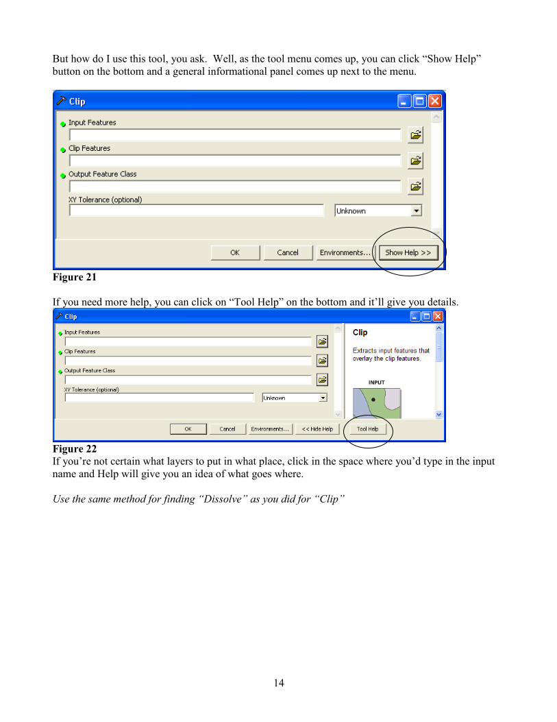
But how do I use this tool, you ask. Well, as the tool menu comes up, you can click “Show Help”

button on the bottom and a general informational panel comes up next to the menu.

Figure 21

If you need more help, you can click on “Tool Help” on the bottom and it’ll give you details.

Figure 22

If you’re not certain what layers to put in what place, click in the space where you’d type in the input

name and Help will give you an idea of what goes where.

Use the same method for finding “Dissolve” as you did for “Clip”