Geoelectrical characterization of a site with hydrocarbon contamination as a result of

pipeline leakage

Omar Delgado-Rodríguez*, Vladimir Shevnin*, Jesús Ochoa-Valdés* and Albert Ryjov** * Instituto Mexicano del Petróleo, México DF. ** Moscow State Geological Prospecting Academy, Russia

Abstract

Resistivity method is used extensively in environmental impact studies. In this work, the results

of the geoelectrical characterization of a hydrocarbons contaminated site are presented. Although

the contamination grade of the site is low, were mapped two contaminated zones into sandy

aquifer. In addition, petrophysical parameters were estimated by recalculate of ground and water

resistivity values in clay content, porosity and CEC values. Anomalous values of clay content,

porosity and CEC indicate the presence of hydrocarbon contaminants. The correlation between

geoelectrical results, petrophysical parameters and hydrocarbons contamination was verified in

laboratory by electrical measurements made in pure and contaminated sand samples.

Key Words: resistivity method, hydrocarbon contamination, geoelectrical characterization,

petrophysical parameters

Resumen

El método de resistividad es ampliamente utilizado en estudios de impacto ambiental. En este

trabajo, se presentan los resultados de la caracterización geoeléctrica de un sitio contaminado por

hidrocarburos. Aunque el grado de contaminación de esta área de estudio es bajo, fue posible

localizar dos zonas contaminadas dentro del acuífero. Además, fueron recalculados los

parámetros petrofísicos contenido de arcilla, porosidad y CIC a partir de los valores de

resistividad de agua y de suelo. Los valores anómalos de contenido de arcilla, porosidad y CIC

indican la presencia de hidrocarburos en el medio. La correlación entre los resultados dados por

los datos geoeléctricos y los parámetros petrofísicos con la presencia de hidrocarburos

contaminantes fue verificada en laboratorio mediante mediciones eléctricas realizadas en

muestras de arena limpia y contaminada.

Palabras Claves: método de resistividad, contaminación por hidrocarburos, caracterización

geoeléctrica, parámetros petrofísicos.

Introduction

Hydrocarbons are the most prevalent type of contaminants in geological media. During the last

decade electrical and electromagnetic methods, especially resistivity method, were applied on the

characterization of oil contaminated soils (Sauck, 1998, 2000). Oil contamination also can be

studied using georadar, self-potential, induced polarization, electromagnetic survey and vertical

resistivity probe (Sauck, 1998).

Recent hydrocarbon contamination gives high resistivity anomalies, while mature oil

contamination produces the low resistivity ones (Sauck, 1998). Several months after the spill has

occurred, contamination creates a low resistivity zone (Sauck, 1998; 2000). The formation

process of a hydrocarbon contaminated area was described in details, linked to chemical reactions

and variations in the physical characteristics of the affected medium (Sauck, 1998; 2000;

Atekwana et al., 2001). According to Sauck, the low resistivity anomaly is resulted of an increase

of Total Dissolved Solids (TDS) due to the acid environment created by the bacterial action in the

inferior part of the vadose zone or below Groundwater Table (GWT).

In this work the application of resistivity method for the characterization of a site with

hydrocarbon contamination as a result of pipeline leakage is presented.

Working site

The evaluation was conducted in an approximately 9,100 m2 site; it’s located near Cárdenas City,

México, where the agriculture is the main use of soil. Four pipelines cross along the site (Fig. 1).

In May of 2002 a hydrocarbon spill from pipeline leakage was registered. After having carried

out an excavation around the spill point and recovered a great part of the poured hydrocarbons,

we decided to realize, as a first step, a soil gas survey and then, a geoelectrical characterization to

assess the soil environmental impact.

Scale in meters 0 10 30 50

-60 -50 -40 -30 -20 -10 0 10 20 30 40 50 60

-20

-10

0

10

20

5

6

543

1

2

LEGEND1 VES profileSpill point Farmed areas

Pipeline

Figure 1: Scheme of the site.

Soil gas survey

The soil gas survey consists of extracting soil gas samples to detect volatile organic compounds

(VOC – that include hydrocarbon) and their concentrations. The results are plotted and latter on

used to have a preliminary idea of coverage and distribution of the hydrocarbons plume.

In November, 2002, was made a soil gas survey based on the measurements of Volatile Organic

Compounds (VOC, ppm). VOC measurements were carried out in situ using a photo ionization

meter. Results were used as a direct indicator of hydrocarbon contamination. Thirty three soil gas

bores were symmetrically distributed around the spilling point (Fig. 2).

VOC values bigger than 2 ppm indicate the existence of volatile compounds associated to

hydrocarbon contamination. Figure 2 shows an anomalous zone with values more than 20,

indicating the migration of contaminants from the spill point to 20 meters toward East (point

CDS-18). Another less remarkable anomalous is detected in the point CDS-21 (50 meters from

spill point). In general, these data indicates that the contamination level is low with a short

horizontal distribution.

2 5 20

-20

-15

-10

-50

5

10

15

2025

CDS-01CDS-02CDS-03CDS-04CDS-05

CDS-06CDS-07CDS-08

CDS-09CDS-10

CDS-11CDS-12CDS-13

CDS-14CDS-15

-64 -56 -48 -40 -32 -24 -16 -8 0 8 16 24 32 40 48 56 64CDS-16

CDS-17 CDS-18 CDS-19 CDS-20 CDS-21 CDS-22

CDS-23 CDS-24 CDS-25

CDS-26 CDS-27

CDS-28 CDS-29 CDS-30

CDS-31 CDS-32

CDS-01

VOC, ppm

LEGEND

Gas boreSpill point Figure 2: Gas oil result.

Geoelectrical Survey

1. - Field-Works

Pipelines location and VES profiles

Using a pipeline locator Fisher TW-6 was possible to locate four pipelines. Taking into account

pipes position, six parallel VES profiles (Fig. 1) were made with a minimal distance from

pipelines of 2.5 m. VES profiles 1 and 2 have 128 m long and profiles 3 to 6 have 104 m long.

Step between VES was 4 m.

VES measurements.

One hundred seventy four VES points were distributed in six profiles (Fig. 1). Due to low

geological noise level Schlumberger array was used taking into account the advantage of its

simplicity and high productivity.

For VES survey we used robust equipment development in our institute that includes a 4.88 Hz

generator with stabilized current (10 to 100 mA) and a measuring instrument with intrinsic noise

of 3*10-7 V. The attenuation of signals for 60 Hz is 10-6 and is more than 10-4 for frequencies

below 0.1 Hz (rejection of fluctuations in self potential on the measuring electrodes).

2. - Qualitative interpretation

Statistical analysis of apparent resistivity data.

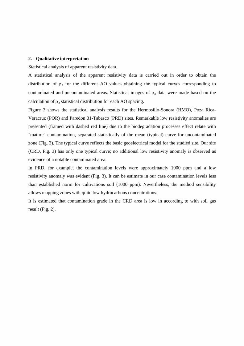
A statistical analysis of the apparent resistivity data is carried out in order to obtain the

distribution of ρa for the different AO values obtaining the typical curves corresponding to

contaminated and uncontaminated areas. Statistical images of ρa data were made based on the

calculation of ρa statistical distribution for each AO spacing.

Figure 3 shows the statistical analysis results for the Hermosillo-Sonora (HMO), Poza Rica-

Veracruz (POR) and Paredon 31-Tabasco (PRD) sites. Remarkable low resistivity anomalies are

presented (framed with dashed red line) due to the biodegradation processes effect relate with

"mature" contamination, separated statistically of the mean (typical) curve for uncontaminated

zone (Fig. 3). The typical curve reflects the basic geoelectrical model for the studied site. Our site

(CRD, Fig. 3) has only one typical curve; no additional low resistivity anomaly is observed as

evidence of a notable contaminated area.

In PRD, for example, the contamination levels were approximately 1000 ppm and a low

resistivity anomaly was evident (Fig. 3). It can be estimate in our case contamination levels less

than established norm for cultivations soil (1000 ppm). Nevertheless, the method sensibility

allows mapping zones with quite low hydrocarbons concentrations.

It is estimated that contamination grade in the CRD area is low in according to with soil gas

result (Fig. 2).

2

3

5

10

15

20

25

ρa, Ohm.m

AO, m

CRD

303745556781

100

10 12 16 202 3 4 5 6 8

Freq., %

3

5

10

15

20

25

30

ρa, Ohm.m

AO, m

POR

Maturecontamination

10

20

2

5

2 10 2051

0

Freq., %

2

5

10

15

20

12

20

33

55

90

148 ρa, Ohm.m

Freq., %

Maturecontamination

10 20 307AO, m 0

HMO

2

4

6

8

10

14

18

22

7.4

12

20

33

55

AO, m

ρa, ohm.m Profiles 6,7,8

2

Mature contamination

PRD

Freq., %

3 4 6 10 14 20

Figure 3: Statistical analysis of apparent resistivity data

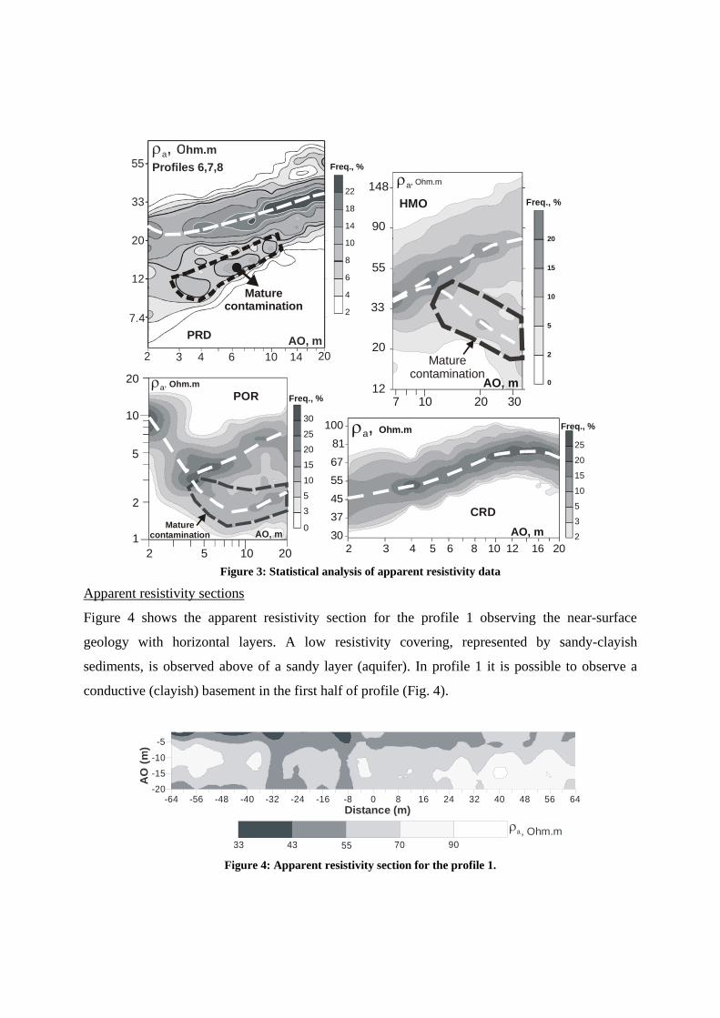
Apparent resistivity sections

Figure 4 shows the apparent resistivity section for the profile 1 observing the near-surface

geology with horizontal layers. A low resistivity covering, represented by sandy-clayish

sediments, is observed above of a sandy layer (aquifer). In profile 1 it is possible to observe a

conductive (clayish) basement in the first half of profile (Fig. 4).

-64 -56 -48 -40 -32 -24 -16 -8 0 8 16 24 32 40 48 56 64-20

-15

-10

-5

33 43 55 70 90, Ohm.mρa

Distance (m)

AO

(m)

Figure 4: Apparent resistivity section for the profile 1.

In the interval -36 m to -8 m of profile 1 the apparent resistivity values for sand layer decrease

(Fig. 4). This low resistivity area is associated with spill happened in pipe next to point 0 m.

Apparent resistivity maps

Apparent resistivity maps show a plan view of resistivity distribution for different study depth. In

AO = 8m map (Fig. 5) is observed a horizontal change of the apparent resistivity. A low

resistivity zone is observed crossing the site with east-west trend. This low resistivity zone can be

the result of two main factors: removed soil by the four pipelines trenches and/or the presence of

contaminants. Last factor can be the cause of the lowest resistivity values.

-64 -56 -48 -40 -32 -24 -16 -8 0 8 16 24 32 40 48 56 64

-10

-5

0

5

10

15

20

25

55 60 70 80ρa (ohm.m)

Figure 5: Apparent resistivity map for AO = 8 m.

3. - Trenches and pipelines effect in the geoelectrical measurements.

By solution of the forward problem it was possible to evaluate the effect of an isolated (resistive)

pipeline (Ryjov and Shevnin, 2001) into a trench less resistive than background (Fig. 6). Model

includes: trench resistivity varying from 1 up to 5 ohm.m, background resistivity 10 ohm.m,

giving the contrast from 0.1 up to 0.5.

109.9

10.0

1 2 3 4 5

D=0.36D=0.50

0.3

ρ=100

ρ=10

AO, m

ρa, Ohm.m

2 203 4 5 6 8

10.5

9.95

2.5

Figure 6: Influence of a conductive trench (trench resistivity value is given in ohm.m for each curve) with diameter 50 cm and depth 30 cm. Inside trench is a pipe with resistivity 100 ohm.m (i.e. insulated).

For trench resistivity 1-3 we have low resistivity anomaly, and for trench resistivity 4-5 ohm.m

there is a small maximal as an influence of an insulated pipe inside the trench (Fig. 6). For actual

resistivity contrast (for example contrast 0.3 and less) an influence of the trench with a pipe is

about 0.1 %. Such influence can be neglected.

4. - Quantitative interpretation

Interpreted resistivity section

A two-dimensional interpretation process using RES2DINV (Loke and Barker, 1996) was

applied to six geoelectrical profiles. In Figure 7 the interpreted section for the profile 1 is

presented. A similar characteristic is observed in all sections: the first half of each profile is

represented by three layers (superficial sandy-clayish, sand and clayish basement), while in the

second half, a more resistive covering (80 ohm.m) than sandy-clayish sediments (40 ohm.m), is

added (Fig. 7).

-64 -56 -48 -40 -32 -24 -16 -8 0 8 16 24 32 40 48 56 64

10

5

0

2.8 7.4 20 55 150, Ohm.mρa

Distance (m)

Dep

th (m

)

Figure 7: Interpreted resistivity section for the profile 1.

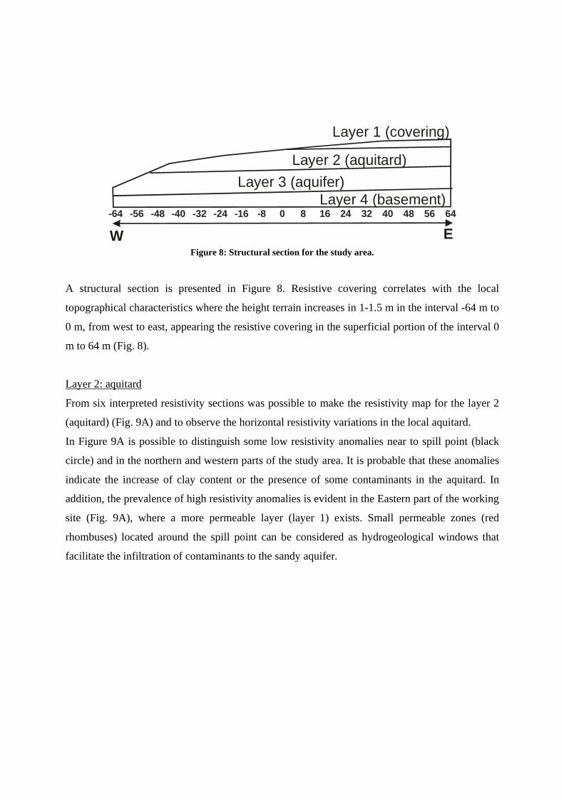
Layer 1 (covering)

Layer 3 (aquifer)Layer 4 (basement)

Layer 2 (aquitard)

W E-64 -56 -48 -40 -32 -24 -16 -8 0 8 16 24 32 40 48 56 64

Figure 8: Structural section for the study area.

A structural section is presented in Figure 8. Resistive covering correlates with the local

topographical characteristics where the height terrain increases in 1-1.5 m in the interval -64 m to

0 m, from west to east, appearing the resistive covering in the superficial portion of the interval 0

m to 64 m (Fig. 8).

Layer 2: aquitard

From six interpreted resistivity sections was possible to make the resistivity map for the layer 2

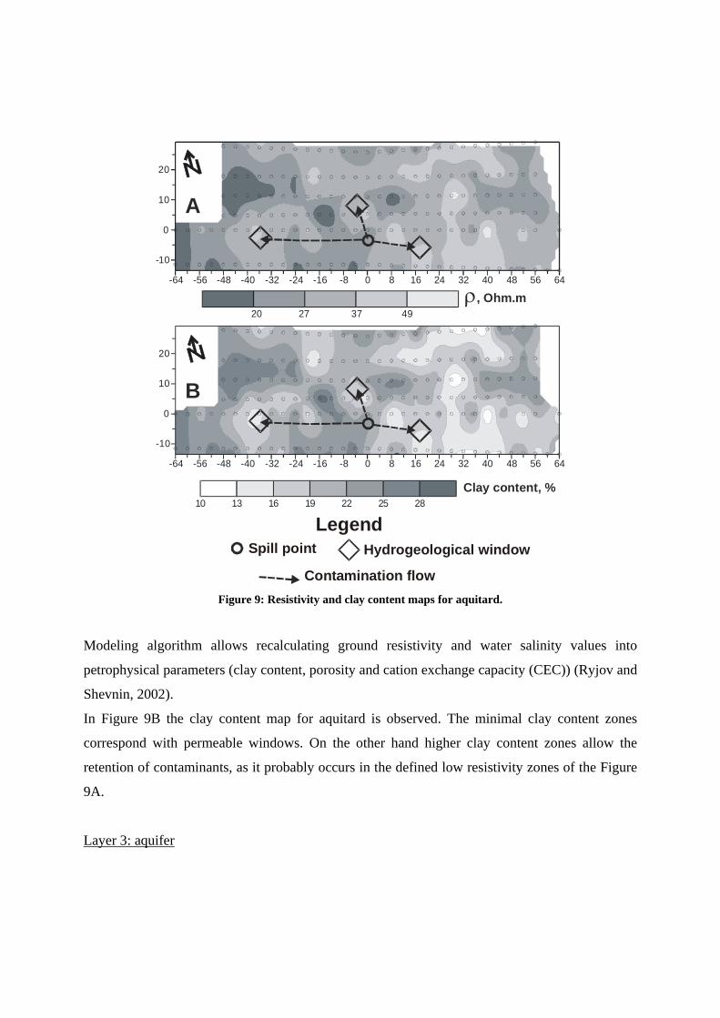
(aquitard) (Fig. 9A) and to observe the horizontal resistivity variations in the local aquitard.

In Figure 9A is possible to distinguish some low resistivity anomalies near to spill point (black

circle) and in the northern and western parts of the study area. It is probable that these anomalies

indicate the increase of clay content or the presence of some contaminants in the aquitard. In

addition, the prevalence of high resistivity anomalies is evident in the Eastern part of the working

site (Fig. 9A), where a more permeable layer (layer 1) exists. Small permeable zones (red

rhombuses) located around the spill point can be considered as hydrogeological windows that

facilitate the infiltration of contaminants to the sandy aquifer.

-64 -56 -48 -40 -32 -24 -16 -8 0 8 16 24 32 40 48 56 64

-10

0

10

20

20 27 37 49ρ, Ohm.m

-64 -56 -48 -40 -32 -24 -16 -8 0 8 16 24 32 40 48 56 64

-10

0

10

20

10 13 16 19 22 25 28Clay content, %

A

B

LegendSpill point Hydrogeological window

Contamination flow Figure 9: Resistivity and clay content maps for aquitard.

Modeling algorithm allows recalculating ground resistivity and water salinity values into

petrophysical parameters (clay content, porosity and cation exchange capacity (CEC)) (Ryjov and

Shevnin, 2002).

In Figure 9B the clay content map for aquitard is observed. The minimal clay content zones

correspond with permeable windows. On the other hand higher clay content zones allow the

retention of contaminants, as it probably occurs in the defined low resistivity zones of the Figure

9A.

Layer 3: aquifer

A similar analysis was made for the sandy aquifer. In Figure 10A resistivities map similar to the

apparent resistivity for AO =8 m (Fig. 5) is shown. Two main anomalous zones are observed:

first anomalous zone cover from the spill point (X = 0 m, Y = -2 m) until X = -40 m, the second

anomalous zone is located to East with coordinated X = 40 – 50 m and y = 8 - 15 m. The origin

of the second anomaly is not clear. It probably can be due to migration and accumulation of

contaminants from the spill point or to be the consequence of a second spill from another pipeline

belonging to the site.

Clay content (Fig. 10B), porosity (Fig. 10C) and CEC (Fig. 10D) maps present a good

correspondence with resistivity map (Fig. 10A). According to our experience, in uncontaminated

zones the petrophysical parameters have true values. In contaminated zones these three

parameters have anomalous values. For example, taking into account the geological information,

clay content is 2%, but in the clay content map (Fig. 10B) we have values up to 6% in anomalous

zones. These anomalous values do not reflect actual changes in clay content, but they reflect

changes in the geoelectrical properties due to contamination.

Petrophysical analysis of contaminated and uncontaminated sand samples.

Figure 11 shows two curves with petrophysical modeling which correspond to an uncontaminated

(white circle) and contaminated (black circle) sand. The petrophysical results obtained for clean

sand were: Clay content: 0 %, Porosity: 32 % and CEC: 0 g/l.

After that, a sand sample was placed in a reactor tank (Fig. 11) with nutrients, bacteria and

petroleum. After several months of biodegradation process the contaminated sand sample gave

the next parameter: Clay content: 10 %, Porosity: 26 % and CEC: 3 g/l. Amplitude changes of

each parameter is similar to that found in sandy aquifer (Clay content 2 to 6%, Porosity 34 to

32% and CEC 1.5 to 3.5 g/l), demonstrating that the anomalous values of clay, porosity and CEC

in the Figure 10 correspond to hydrocarbons contaminated zones. So, we found an important

effect that allows locating contaminated zones.

-64 -56 -48 -40 -32 -24 -16 -8 0 8 16 24 32 40 48 56 64

-10

0

10

20

148 200 270 365 493ρ, Ohm.m

-64 -56 -48 -40 -32 -24 -16 -8 0 8 16 24 32 40 48 56 64

-10

0

10

20

1 2 3 4 5 6Clay content, %

-64 -56 -48 -40 -32 -24 -16 -8 0 8 16 24 32 40 48 56 64

-10

0

10

20

32.5 33 33.5 34Porosity, %

-64 -56 -48 -40 -32 -24 -16 -8 0 8 16 24 32 40 48 56 64

-10

0

10

20

2 2.5 3CEC, g/l

A

B

C

D

LegendSpill point Hydrogeological window

Contamination flow Main anomalous zone Figure 10: Comparative (A) resistivity, (B) clay content, (C) porosity and (D) CEC maps for sandy aquifer.

1 10 100

C(NaCl), g/l

ρ, Ohm.m

Water

2030

405070100

0.1

1

10

20

T=20Co

CEC=3Clay

30

Before contaminationAfter contamination

CHANGES IN REACTOR1.- Clay content: 0 to 10%2.- CEC: 0 to 3 g/l3.- Porosity: 32 to 26%

Figure 11: Calculation of petrophysical parameters for sand (before and after contamination).

Conclusions

Resistivity sounding method is effective for geoelectrical characterization of contaminated zones,

allowing future geochemical study with an optimized wells location and drilling depths.

The contamination of the study area is low. Only two zones have notice anomalies: the first one

associated with spill point and the second one located in the Eastern portion of the study area.

The local aquifer (sandy layer) is protected of the contamination by a superficial clayish layer.

Nevertheless, in areas where the clay content decrease or trenches related with pipelines are

presented the vulnerability is increased, facilitating the infiltration of contaminants to aquifer, as

it happened in the interval X = -36 to -8 m of profile 1.

Changes of soil properties in the sandy aquifer and in the reactor tank were very similar.

Recalculation of petrophysical parameters from VES resistivity and groundwater salinity helps

characterizing uncontaminated and contaminated zones.

References

Atekwana E.A., Cassidy D.P., Magnuson C., Endres A.L., Werkema D.D., Jr. and Sauck W.A.,

2001: Changes in geoelectrical properties accompanying microbial degradation of LNAPL.

SAGEEP proceedings, OCS_1.

Loke, M.H. and Barker, R.D., 1996: Rapid least-squares inversion of apparent resistivity

pseudosections by a quasi-Newton method. Geophysical Prospecting, 44, 131-152.

Ryjov A. and Shevnin V., 2001: Anomalies from horizontal metal pipes in resistivity and IP

fields. SAGEEP proceedings. ERP_4, 8 pp.

Ryjov, A. and Shevnin, V., 2002: Theoretical calculation of rocks electrical resistivity and some

examples of algorithm's application. SAGEEP proceedings, P2, 10 pp.

Sauck W. A., 1998: A conceptual model for the geoelectrical response of LNAPL plumes in

granular sediments. SAGEEP Proceedings, 805-817.

Sauck, W. A., 2000: A model for the resistivity structure of LNAPL plumes and their environs in

sandy sediments. J. App. Geophys., 44, 151–165.