Chaotic Modeling and Simulation (CMSIM) : 281–298, 2012

Geodesics Revisited

Pavel Pokorny

Prague Institute of Chemical Technology, Prague, Czech Republic(E-mail: pavel.pokorny@vscht.cz)

Abstract. Metric tensor and Christoffel symbols are revised and the equation ofgeodesic is derived from two possible definitions: based on zero tangent accelerationand on minimal length. Geodesics on a torus are shown to split into two distinctclasses. Dynamical systems approach is used to investigate these two classes. Appli-cation of geodesics in optics and in mechanics are given.Keywords: dynamical system, geodetic, torus.

1 Introduction

In Euclidean space a segment of a line is the shortest connection of two givenpoints. The segment has also the property that a point moving along thesegment with velocity of constant magnitude has zero acceleration. A geodesic(a geodesic curve) is a generalization of the term segment for spaces that arenot Euclidean. An example of such a space is a two dimensional surface in athree dimensional Euclidean space.

Historically perhaps the oldest example of such a surface is the sphere (thesurface of a ball) because our space for living was limited to the surface of theEarth for a long time. Here comes the origin of the word geodesic. Geo- is thefirst part of compound words meaning the Earth.

These curved surfaces can be studied in two ways. Either as subsets of anEuclidean space of higher dimension, or as independent curved spaces withoutany reference to a higher dimensional Euclidean space. The intrinsic geometryof such a curved space can be described by certain matrix depending on thepoint in the space. This matrix function is called the metric tensor. A spacewith a constant metric tensor is called a flat (Euclidean) space, while a spacewith a non-constant metric tensor is called a curved space.

In chapter 2 a metric tensor is introduced and its examples for a sphere andfor a torus are given.

In chapter 3 the geodesic is defined as the curve such that a point movingalong the curve with the velocity of constant magnitude (i.e. the velocitycan change its direction but not its magnitude) has the acceleration vectorperpendicular to the given surface, i.e. the acceleration component tangent tothe given surface is zero. Such a motion can be expressed by a non-scientific

Received: 17 July 2011 / Accepted: 27 December 2011c© 2012 CMSIM ISSN 2241-0503

282 P. Pokorny

expression “follow your nose”. Given this condition the equation of geodesicis derived. It is a second order differential equation for the functions thatparametrically describe the curve.

In chapter 4 alternatively the geodesic is defined as the shortest curve be-tween two given points. Given this condition the same equation of geodesic isderived.

In chapter 5 we show that the magnitude of velocity remains constant forthe solution of the equation of geodesic.

In chapter 6 the first integral (i.e. a constant function of state variables) isderived for certain simplified cases.

In chapter 7 the equation of geodesic is applied for a sphere. We show thatgeodesics on a sphere are the great circles i.e. the circles with the center in thecenter of the sphere.

In chapter 8 geodesics on a torus are investigated. The geodesics on atorus fall into two classes. Roughly speaking, one class contains geodesics thatremain mainly on the outer part of the torus (see Fig. 6) while the other classcontains geodesics that wind around the tube of the torus along a spiral (seeFig. 7). Another difference between these two classes is that a geodesic in thefirst class is either closed or it has self-intersections, while a geodesic in theother class is either closed or it has no self-intersections.

In chapter 9 a physical application of geodesics is given, namely the prop-agation of light in optically non-homogeneous medium, i.e. where the indexof refraction depends on the point in the space. We find the metric tensorappropriate for investigation of the shape of the light ray and the Snell law ofrefraction is derived from the equation of geodesic found in chapter 3 and 4.This example is interesting in that it is convenient to replace the three dimen-sional Euclidean space by a curved space described by a non-constant metrictensor for the study of the propagation of light (or in general any wave withvarying speed).

In chapter 10 the results of chapter 9 are applied for the study of theshape of the path that brings a mass point from a given initial point to anothergiven point in the shortest possible time (assuming a homogeneous gravitationalfield). This path is called a brachistochrone and we show that it can be foundas a geodesic with appropriate metric tensor.

There are many more examples of geodesics. Besides being an interestingmathematical question of its own, they have many physical and technologicalapplication. Spanning from general relativity to cases that seem to have nothingin common with mathematics or physics such as winding a ribbon round handle-bars of a bicycle or dressing an injured knee.

Geodesics are sometimes illustrated as the equilibrium position of a springon a slippery surface. This is a good example for convex parts of the surface;near concave parts of the surface a real spring would go through the air whilethe geodesic must stay in the given surface. To see this, imagine a thin rubberaround an apple. There is a little pit near the stem of the apple. The rubbercrosses this pit through the air which the geodesic is not allowed to do.

Chaotic Modeling and Simulation (CMSIM) : 281–298, 2012 283

2 Metric tensor

Consider a M -dimensional manifold embedded into a N -dimensional Euclideanspace with parametric equations

y = r(x),

where r : RM → RN .E.g. a sphere with unit radius can be given by

y1 = r1(x1, x2) = r1(ϑ, ϕ) = sinϑ cosϕ (1)

y2 = r2(x1, x2) = r2(ϑ, ϕ) = sinϑ sinϕ

y3 = r3(x1, x2) = r3(ϑ, ϕ) = cosϑ

and a torus by

y1 = r1(x1, x2) = r1(u, v) = (a+ cosu) cos v (2)

y2 = r2(x1, x2) = r2(u, v) = (a+ cosu) sin v

y3 = r3(x1, x2) = r3(u, v) = sinu,

where a > 1 is the radius of the axis of the tube; the radius of the tube being 1.The comma before an index will denote the partial derivative with respect

to the variable given by the index after the comma. Thus e.g. for rk (the k-thcomponent of the vector r) its partial derivative is

rk,i =∂rk∂xi

.

Then the differential of y isdyk = rk,idxi

(we sum over each index appearing twice in a product) and the square of itsnorm is

||dy||2 = dykdyk = rk,irk,jdxidxj = gijdxidxj ,

wheregij = rk,irk,j (3)

are the components of the metric tensor.E.g. for a sphere putting (1) into (3) gives

g =

(1 00 sin2 ϑ

)and for a torus putting (2) into (3) gives

g =

(1 00 (a+ cosu)2

).

Later we will need another relation between g and r. We can differentiate

gij(x) = rm,i(x)rm,j(x)

284 P. Pokorny

with respect to xk to yield

gij,k = rm,ikrm,j + rm,irm,jk.

We add and subtract to this equation its two cyclic permutations

gjk,i = rm,ijrm,k + rm,jrm,ik.

gki,j = rm,kjrm,i + rm,krm,ij

and we getgij,k + gjk,i − gki,j = 2rm,ikrm,j .

3 Geodesic as the curve with zero tangent acceleration

Consider a curveα = α(t) = r(x(t)),

where α : I → RN is a sufficiently smooth function, I is the interval I = [t1, t2].When we call t the time, we can call

αk(t) = rk,ixi(t)

the velocity andαk(t) = rk,ij xixj + rk,ixi.

the acceleration. We want to find the shape of the curve, so that the accelera-tion has zero projection to the plane tangent to the given surface

αkrk,n = 0 for n = 1, . . . ,M

(rk,ij xixj + rk,ixi)rk,n = 0

rk,irk,nxi + rk,ijrk,nxixj = 0

ginxi +1

2(gin,j + gnj,i − gji,n)xixj = 0.

It is convenient to denote gnm the element of the inverse matrix to the matrixwith elements gin (i.e. ging

nm = δim is the element of the unit matrix). Then

xm +1

2gnm(gin,j + gnj,i − gji,n)xixj = 0

and finallyxm + Γmij xixj = 0, (4)

where

Γmij =1

2gnm(gin,j + gnj,i − gji,n) (5)

is called the Christoffel symbol.From (3) it follows that the metric tensor g is symmetric, i.e.

gij = gji

Chaotic Modeling and Simulation (CMSIM) : 281–298, 2012 285

and as a result the Christoffel symbol is also symmetric

Γmij = Γmji .

We call (4) the equation of geodesic. In this equation the properties of thesurface appear only through the metric tensor g and its derivatives (via theChristoffel symbol Γmij ). This allows us to work in the M -dimensional spacewith the metric g without any reference to the N -dimensional Euclidean space.

If the metric tensor g as a function of the point in the space is constant,its derivatives vanish and so do all the Christoffel symbols. The equation ofgeodesic is then

xm = 0

and the geodesic is the straight line in this special case.

4 Geodesic as the shortest curve

Consider a curvex = α(t)

where α : I → Rn is a sufficiently smooth function and the interval I is I =[t1, t2].

If g is the metric tensor, then the magnitude of the velocity of a pointtraveling along the curve α is

vα(t) =√gij(α(t)) αi(t) αj(t).

Let us denote

V (x1, . . . , xn, x1, . . . , xn) =√gij(x1, . . . , xn) xi xj

in short

V (x, x) =√gij(x) xi xj . (6)

Similarly we will write α instead of α1, . . . , αn and α instead of α1, . . . , αn.Then the length of the curve α is

L(α) =

t2∫t1

vα(t) dt =

t2∫t1

V (α(t), α(t)) dt.

For ε ∈ R and β : I → Rn such that β(t1) = β(t2) = 0 we denote

L(ε) = L(α+ εβ) =

t2∫t1

V (α(t) + εβ(t), α(t) + εβ(t)) dt

and

L′(ε) =dL

dε.

286 P. Pokorny

We want

L′(0) = 0,

meaning that a small change in the shape of the curve does not make it shorter.Thus

0 =

t2∫t1

(Vxiβi + Vxi βi) dt.

We integrate by parts and we use the assumption β(t1) = β(t2) = 0 (meaningthat the start point and the end point of the curve are fixed) to get

0 =

t2∫t1

(Vxiβi − Vxi

βi) dt =

t2∫t1

(Vxi− Vxi

)βi dt.

This must hold for arbitrary functions βi, thus the bracket must vanish

Vxi− Vxi

= 0 for i = 1, . . . , n,

thus

Vxi − (Vxixkxk + Vxixk

xk) = 0. (7)

To get a unique solution we add the assumption of constant magnitude of thevelocity

V = 0 (8)

thus

Vxkxk + Vxk

xk = 0. (9)

When putting (6) into (7) and using (9) the same equation of geodesic (4) isderived. To do it by hand it is convenient to introduce W by

W (x, x) = gij(x) xi xj (10)

i.e.

V =√W. (11)

Putting (11) into (7) yields

2WWxmxsxs + 2WWxmxr

xr −Wxm(Wxs

xs +Wxrxr) = 2WWxm

(12)

where the bracket vanishes because of (9) and (11). When we substitute Wfrom (10) into (12) we get again the equation of geodesic

xm + Γmij xixj = 0,

where

Γmij =1

2gnm(gin,j + gnj,i − gji,n).

Chaotic Modeling and Simulation (CMSIM) : 281–298, 2012 287

5 Constant magnitude of velocity

We have used the assumption of constant magnitude of velocity (8) to simplify(12). It is not clear, however, whether the solution of the resulting equation ofgeodesic (4) still satisfies the condition (8). We show it does. Let us write theequation of geodesic (4) as a system of first order ODE’s

xm = Xm (13)

Xm = −Γmij XiXj .

The condition of constant square of the magnitude of velocity

W = gij(x) xi xj = gij(x) Xi Xj = const.

is the equation of a hyper-surface in the state space (of twice the dimension).It is easy to show that the vector field f of (13) is orthogonal to the gradientof W

f · ∇W =

(Xm

−Γmij XiXj

)·(gij,mXiXj

2gmkXk

)=

= gij,mXiXjXm − 2gmkΓmij XiXjXk =

= gij,mXiXjXm − gmkgnm(gin,j + gnj,i − gji,n)XiXjXk =

= gij,mXiXjXm − (gin,j + gnj,i − gji,n)XiXjXn = 0.

Thus the square of the magnitude of velocity is constant and so is the magnitudeitself.

6 First integral

In this chapter we rewrite the equation of geodesic (4) for special cases andthen we find its first integral.

Assuming dimension 2, denoting x1 = x, x2 = y and assuming a diagonalmetric tensor g, i.e. g12(x, y) = g21(x, y) = 0 we arrive at

x+g11,12g11

xx+g11,2g11

xy − g22,12g11

yy = 0 (14)

y − g11,22g22

xx+g22,1g22

xy +g22,22g22

yy = 0. (15)

Further, assuming that g depends on x only and not on y, formally written

,2 = 0 meaning ∂∂y = 0 or g11,2 = g22,2 = 0 we get even more simple equations

x+g11,12g11

xx− g22,12g11

yy = 0 (16)

y +g22,1g22

xy = 0. (17)

We will use this result (assuming further g11 = g22) in chapter 9.

288 P. Pokorny

In chapters 7 and 8 we will work with the metric tensor where one of itsdiagonal elements is constant. Assuming g11(x, y) = 1 allows us to simplify theequation of geodetic even more

x− g22,12

yy = 0 (18)

y +g22,1g22

xy = 0. (19)

Now we can find the first integral of this system of ODE’s. Multiplying (18)by y and multiplying (19) by x and subtracting the second equation from thefirst one we get

xy − yx− g22,12

y3 − g22,1g22

x2y = 0.

When multiplying this equation by 2xg222y

3 we get (after simple manipulation)

d

dt

(1

g22(x(t))2(x

y)2 +

1

g22(x(t))

)= 0

which is equivalent to1

g222(dx

dy)2 +

1

g22= const. (20)

We will use this first integral of the equation of geodesic in chapters dealingwith the sphere and with the torus.

7 Geodesics on a sphere

Putting x1 = ϑ, x2 = ϕ and

g =

(1 00 sin2 ϑ

)into the equation of geodesic (4) yields

ϑ− sinϑ cosϑ ϕ2 = 0

ϕ+ 2 cotϑ ϕ ϑ = 0.

Its first integral (20) is

1

sin4 ϑ

(dϑ

dϕ

)2

+1

sin2 ϑ=

1

sin2 ϑ0, (21)

where ϑ0 = min(ϑ) and ϕ0 are the coordinates of “the north most” point ofthe curve.

This is the equation of a circle lying in the plane going through the origin.Such a plane has the equation

x · xP = 0,

Chaotic Modeling and Simulation (CMSIM) : 281–298, 2012 289

where

x =

sinϑ cosϕsinϑ sinϕ

cosϑ

and

xP =

sinϑP cosϕPsinϑP sinϕP

cosϑP

where

ϕP = ϕ0 + π, ϑP =π

2− ϑ0

are coordinates of the normal vector to the plane. After some manipulation

ϕ = ϕ0 + arccos (tanϑ0 cotϑ).

Differentiating gives

dϕ

dϑ=

1

sin2 ϑ

tanϑ0√1− (tanϑ0 cotϑ)2

and1

sin4 ϑ(dϑ

dϕ)2 =

1

sin2 ϑ0− 1

sin2 ϑ

which agrees with(21).

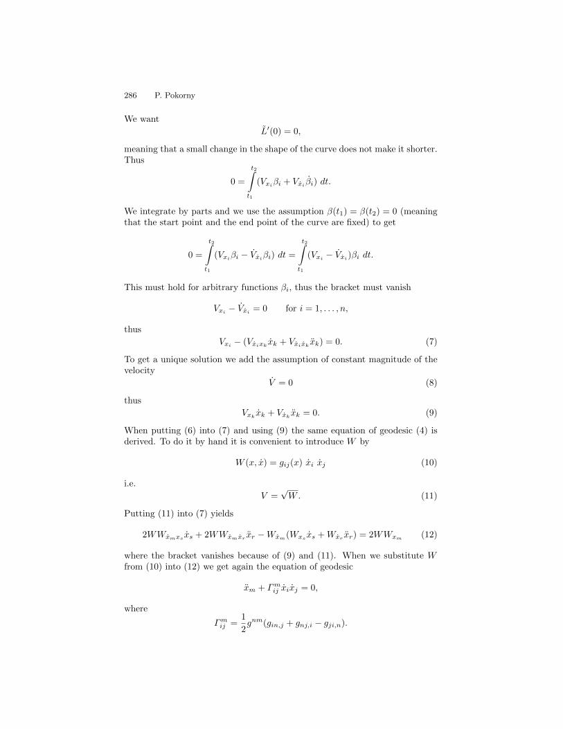
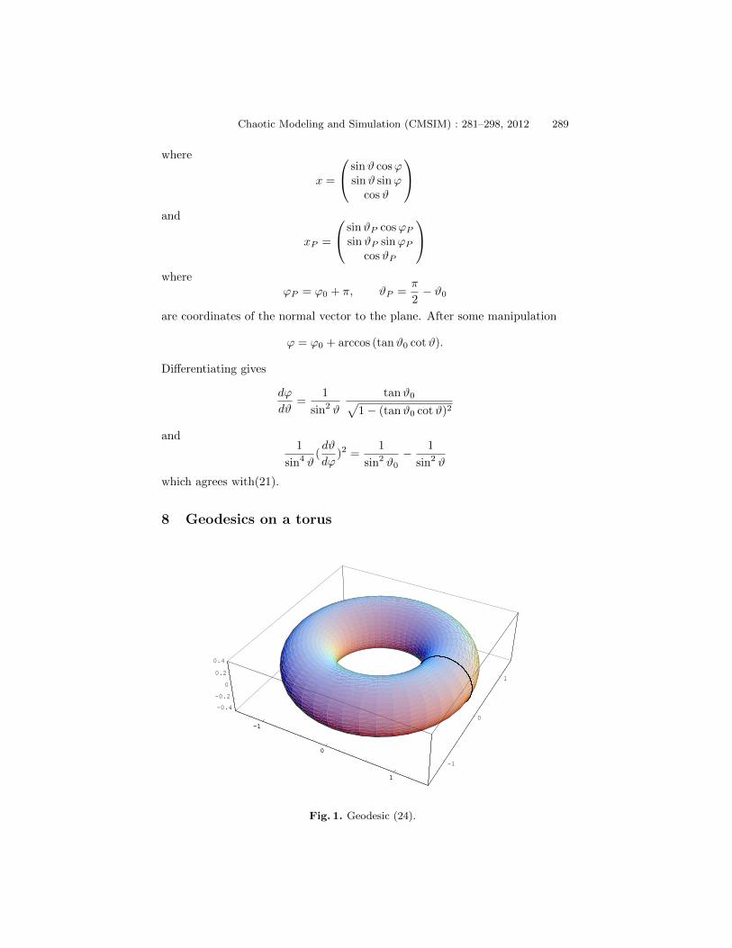
8 Geodesics on a torus

-1

0

1

-1

0

1

-0.4

-0.2

0

0.2

0.4

-1

0

1

Fig. 1. Geodesic (24).

290 P. Pokorny

-1

0

1

-1

0

1

-0.4

-0.2

0

0.2

0.4

-1

0

1

Fig. 2. Geodesic (25).

-1

0

1

-1

0

1

-0.4

-0.2

0

0.2

0.4

-1

0

1

Fig. 3. Geodesic (26).

Substituting x1 = u, x2 = v, and the metric tensor

g =

(1 00 (a+ cosu)2

)(22)

into the equation of geodesic (4) gives

u+ (a+ cosu) sinu v2 = 0

v − 2sinu

a+ cosuu v = 0.

Chaotic Modeling and Simulation (CMSIM) : 281–298, 2012 291

-5

0

5

u-5

0

5

d

0

5

10

f

-5

0

5

u

Fig. 4. The graph of the function (29) shows the minimum for (u, d) = (0, 0) and asaddle for (u, d) = (π, 0).

This system of two differential equations of the second order can be writtenas a system of four equations of the first order

u = U (23)

U = −(a+ cosu) V 2 sinu

v = V

V = 2sinu

a+ cosuU V.

The 4 dimensional state space (u, U, v, V ) of this system is divided by thehyper-plane V = 0 into two half-spaces. The hyper-plane V = 0 contains thesolution

u = k1t+ k2 (24)

U = k1

v = k3

V = 0,

where k1, k2, k3 ∈ R.Corresponding to each solution in one half-space there is one solution in

the other half-space. These two solutions are symmetrical with respect to thehyper-plane V = 0. The theorem of the uniqueness of solution implies thatV (t) is either always positive or always zero or always negative. Meaning thesolutions neither cross nor touch the hyper-plane V = 0. Thus we can limitour attention to solutions satisfying V (t) = v(t) > 0.

292 P. Pokorny

-6 -4 -2 0 2 4 6

-7.5

-5

-2.5

0

2.5

5

7.5

u

d

Fig. 5. The contour-lines of the function (29) are closed curves near a minimum.A separatrix (shown in red) going from the saddle separates a region with closedcontour-lines from the region with non-closed contour-lines. Closed contour-linescorrespond to geodesics that remain mainly in the outer part of the torus (see Fig. 6).Non-closed contour-lines correspond to geodesics that wind around the tube of thetorus (see Fig. 7).

Among these solutions there are two special solutions satisfying u(t) = 0,namely

u = 0 (25)

U = 0

v = k1t+ k2

V = k1,

and

u = π (26)

U = 0

v = k1t+ k2

V = k1.

The behavior of nearby trajectories can be studied by linear expansion.The Jacobi matrix of partial derivatives of the system (23) evaluated on the

Chaotic Modeling and Simulation (CMSIM) : 281–298, 2012 293

trajectory (25) has two zero eigenvalues and two purely imaginary complexconjugate eigenvalues

λ3,4 = ±ik1√a+ 1. (27)

This means it acts like a center; nearby trajectories rotate around it in the u-Uplane spanned by the corresponding eigenvectors.

The Jacobi matrix of partial derivatives of the system (23) evaluated on thetrajectory (26) has two zero eigenvalues and two real eigenvalues with oppositesigns

λ3,4 = ±k1√a− 1.

Thus the trajectory (26) is a saddle with one stable and one unstable directionsin the u-U plane. The saddle itself is not a stationary point but rather a closedtrajectory. In fact, there are no stationary points, the velocity has a constantmagnitude.

The first integral (20) for torus is

1

(a+ cosu)4(du

dv)2 +

1

(a+ cosu)2= const. (28)

Thus geodesics on a torus can be described by contour-lines of the function

f(u, d) =1

(a+ cosu)4(d)2 +

1

(a+ cosu)2. (29)

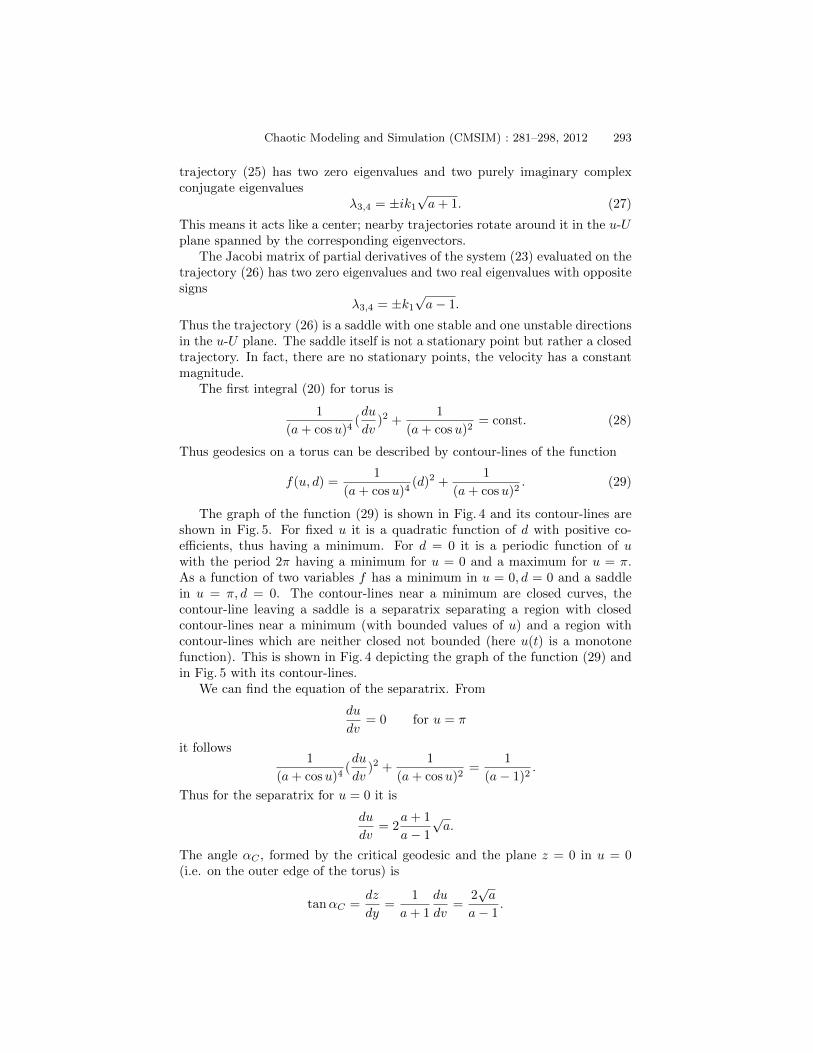
The graph of the function (29) is shown in Fig. 4 and its contour-lines areshown in Fig. 5. For fixed u it is a quadratic function of d with positive co-efficients, thus having a minimum. For d = 0 it is a periodic function of uwith the period 2π having a minimum for u = 0 and a maximum for u = π.As a function of two variables f has a minimum in u = 0, d = 0 and a saddlein u = π, d = 0. The contour-lines near a minimum are closed curves, thecontour-line leaving a saddle is a separatrix separating a region with closedcontour-lines near a minimum (with bounded values of u) and a region withcontour-lines which are neither closed not bounded (here u(t) is a monotonefunction). This is shown in Fig. 4 depicting the graph of the function (29) andin Fig. 5 with its contour-lines.

We can find the equation of the separatrix. From

du

dv= 0 for u = π

it follows1

(a+ cosu)4(du

dv)2 +

1

(a+ cosu)2=

1

(a− 1)2.

Thus for the separatrix for u = 0 it is

du

dv= 2

a+ 1

a− 1

√a.

The angle αC , formed by the critical geodesic and the plane z = 0 in u = 0(i.e. on the outer edge of the torus) is

tanαC =dz

dy=

1

a+ 1

du

dv=

2√a

a− 1.

294 P. Pokorny

-1

0

1

-1

0

1

-0.4

-0.2

0

0.2

0.4

-1

0

1

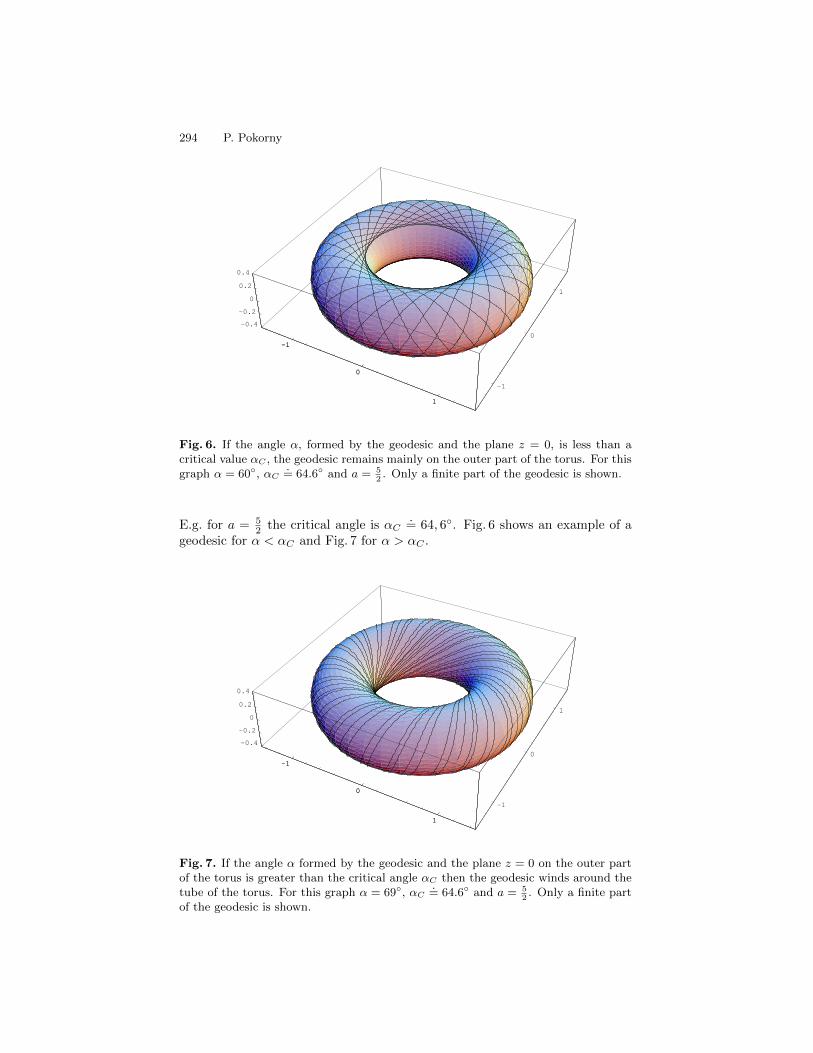
Fig. 6. If the angle α, formed by the geodesic and the plane z = 0, is less than acritical value αC , the geodesic remains mainly on the outer part of the torus. For thisgraph α = 60◦, αC

.= 64.6◦ and a = 5

2. Only a finite part of the geodesic is shown.

E.g. for a = 52 the critical angle is αC

.= 64, 6◦. Fig. 6 shows an example of a

geodesic for α < αC and Fig. 7 for α > αC .

-1

0

1

-1

0

1

-0.4

-0.2

0

0.2

0.4

-1

0

1

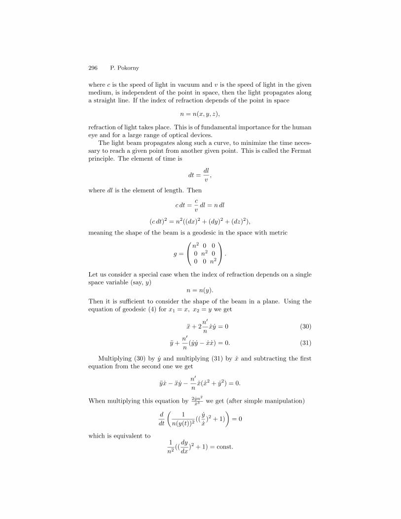
Fig. 7. If the angle α formed by the geodesic and the plane z = 0 on the outer partof the torus is greater than the critical angle αC then the geodesic winds around thetube of the torus. For this graph α = 69◦, αC

.= 64.6◦ and a = 5

2. Only a finite part

of the geodesic is shown.

Chaotic Modeling and Simulation (CMSIM) : 281–298, 2012 295

Are the geodesics on a torus closed curves? From (28) it follows that u as afunction of v is periodic for small u (i.e. for u0 < π). Let us denote its period T .If T is a rational multiple of 2π (as the increase of v by 2π corresponds to thesame point) then the geodesic is a closed curve. The period T can be evaluatedas follows. From (28) we find

dv =a+ cosu0

(a+ cosu)√

(a+ cosu)2 − (a+ cosu0)2du

and

T = 4

u0∫0

a+ cosu0

(a+ cosu)√

(a+ cosu)2 − (a+ cosu0)2du.

It is sufficient to integrate over one quarter of the period because the func-tion (29) is even in both u and d.

The period T is a continuous function of two variables: a (the ratio of theradius of the axis of the tube of the torus and the radius of the tube of thetorus) and u0 (maximum of u on the geodesic) thus

T = T (a, u0).

When a or u0 is varied continuously then the ratio T2π will achieve rational and

irrational values and in every neighborhood of a closed geodesic there will beinfinitely many non-closed ones and vice versa. Almost every geodesic will benon-closed.

It is possible to compute the period T (a, u0) for small amplitude u0

limu0→0

T (a, u0) =2π√a+ 1

,

so that e.g. for a = 3 the geodesic for small u0 will almost close after two turnsaround the torus. This is in agreement with (27).

Our results in this chapter differ from the classical ones based on the in-trinsic geometry of the torus T 2 = R2/N inherited from the Euclidean plane(u, v), where the geodesics are straight lines in the plane (u, v) and thus havingthe constant slope. When wound on the torus a geodesic is either a closedcurve or it fills densely the entire surface of the torus. We, however, assumethe metric tensor (22) based on the geometry of the torus as embedded into athree dimensional Euclidean space. This non-constant metric tensor gives riseto two distinct classes of geodesic curves (cf. Fig. 6 and Fig. 7).

9 Geodesic as the light beam

If the optical index of refraction

n =c

v,

296 P. Pokorny

where c is the speed of light in vacuum and v is the speed of light in the givenmedium, is independent of the point in space, then the light propagates alonga straight line. If the index of refraction depends of the point in space

n = n(x, y, z),

refraction of light takes place. This is of fundamental importance for the humaneye and for a large range of optical devices.

The light beam propagates along such a curve, to minimize the time neces-sary to reach a given point from another given point. This is called the Fermatprinciple. The element of time is

dt =dl

v,

where dl is the element of length. Then

c dt =c

vdl = ndl

(c dt)2 = n2((dx)2 + (dy)2 + (dz)2),

meaning the shape of the beam is a geodesic in the space with metric

g =

n2 0 00 n2 00 0 n2

.

Let us consider a special case when the index of refraction depends on a singlespace variable (say, y)

n = n(y).

Then it is sufficient to consider the shape of the beam in a plane. Using theequation of geodesic (4) for x1 = x, x2 = y we get

x+ 2n′

nxy = 0 (30)

y +n′

n(yy − xx) = 0. (31)

Multiplying (30) by y and multiplying (31) by x and subtracting the firstequation from the second one we get

yx− xy − n′

nx(x2 + y2) = 0.

When multiplying this equation by 2yn2

x3 we get (after simple manipulation)

d

dt

(1

n(y(t))2((y

x)2 + 1)

)= 0

which is equivalent to1

n2((dy

dx)2 + 1) = const.

Chaotic Modeling and Simulation (CMSIM) : 281–298, 2012 297

1

n2(dl)2

(dx)2= const.

1

n21

sin2 α= const.

and finallyn sinα = const (32)

where α is the angle formed by the beam and the normal vector to the planeof constant index of refraction.

A special case

n(y) =1

y

i.e.

g =

( 1y2 0

0 1y2

)for y > 0 is called the Poincare metric. Then (32) gives

1

ysinα = K.

Comparing with the equation of a circle with radius R

sinα =y

R

shows that the geodesics in Poincare metric are semicircles for K = 1R > 0 and

straight linesα = 0

i.e.x = const.

for K = 0.

10 Brachistochrone

Brachi- is the first part of compound words meaning short and chronos meanstime. Brachistochrone is the name for the curve bringing a mass point froma given point to another given point in the shortest possible time (assuminghomogeneous gravitational field). To find it we make use of the results fromthe previous chapter.

The conservation of mechanical energy

1

2mv2 +mgh = mgh0

lets us introduce a quantity playing a similar role as the index of refraction forlight

n =c

v=

const√y0 − y

.

298 P. Pokorny

Using the law of refractionn sinα = const

we getsinα√y0 − y

= const.

When we describe the curve as the graph of a function

y = y(x)

we get the equation(1 + y′2)(y0 − y) = const.

It is easy to show that this is the cycloid. Starting with the parametricequation of cycloid

x = Rωt+R cosωt

y = R sinωt

and differentiating with respect to time

x = Rω −Rω cosωt

y = Rω cosωt

we find

y′2 = (y

x)2 =

cos2 ωt

(1− sinωt)2

and(1 + y′2)(y0 − y) = 2R = const.

Meaning that the cycloid is also a geodesic with a suitable metric.

References

1.Arnold V. I.: Ordinary Differential Equations. MIT Press 1998.2.Horsky J. et al.: Mechanika ve fyzice. Academia Prague 2001.3.Ljusternik L. A.: Kratcajsije linii. Gostechizdat Moscow 1955.