ITK Deformable Registration B-Splines Free-Form. Deformable Registration.

Journal of Mathematical Imaging and Visionc© 2006 Springer Science + Business Media, Inc. Manufactured in The Netherlands.
DOI: 10.1007/s10851-005-3624-0
Geodesic Shooting for Computational Anatomy
MICHAEL I. MILLERCenter of Imaging Science & Department of Biomedical Engineering, The John Hopkins University,
301 Clark Hall, Baltimore, MD 21218, [email protected]
ALAIN TROUVECMLA, ENS de Cachan, 61 Avenue du President Wilson, 94235 Cachan CEDEX, France
LAURENT YOUNESCenter for Imaging Science & Department of Applied Math and Statistics, The Johns Hopkin, 3245 Clark Hall,
Baltimore, MD 21218, [email protected]
Published online: 28 January 2006
Abstract. Studying large deformations with a Riemannian approach has been an efficient point of view togenerate metrics between deformable objects, and to provide accurate, non ambiguous and smooth matchingsbetween images. In this paper, we study the geodesics of such large deformation diffeomorphisms, and moreprecisely, introduce a fundamental property that they satisfy, namely the conservation of momentum. This propertyallows us to generate and store complex deformations with the help of one initial “momentum” which serves as theinitial state of a differential equation in the group of diffeomorphisms. Moreover, it is shown that this momentumcan be also used for describing a deformation of given visual structures, like points, contours or images, andthat, it has the same dimension as the described object, as a consequence of the normal momentum constraint weintroduce.
1. Introduction
Over the past several years we have been studyingnatural shapes using homogeneous orbits of imageryconstructed via the action of transformation groups onexemplars or templates. The mathematical structure ofgroup action as a model in image analysis has been pi-oneered by Grenander [13], the idea being to introducethe group actions in the very nature of the objects them-selves, through the notion of deformable templates.Roughly speaking, a deformable template simply is an“object or exemplar” Itemp on which a group G acts
and generates, through the orbit J = G · Itemp, a wholefamily of new objects. The interest of this approach isto concentrate the modeling effort on the group G, andnot on the family of objects J .
Since the earliest introduction by Silicon GraphicsIncorporated of special purpose graphics hardware forobject rendering, group action as a model in imageanalysis has been the subject of a wide range of re-search in computer vision. Naturally, the analyticaland computational properties of the low-dimensionalmatrix Lie groups form the core dogma of modernComputer graphics. In sharp contrast, however, for the

Miller, Trouve and Younes
study of imagery generated from natural or biologi-cal shapes, the finite dimensional matrix groups arereplaced by their infinite dimensional analogue, themore general diffeomorphisms [7, 11, 16, 22, 23, 36].
The anatomical orbit or deformable template is madeinto a metric space with a metric distance between el-ements by constructing curves through the space ofdiffeomorphisms connecting them; the length of thecurve becomes the basis for the construction, the metricdistance corresponding to the geodesic shortest lengthcurves. This gives rise to a natural variational prob-lem describing the geodesic flows between elementsin the orbit, with the solution of the associated Euler-Lagrange equations giving the optimal flow of diffeo-morphisms and thus the metric between the shapes.The obtained setting shares several similarities withthe mechanics of perfect fluids, for which the Euler-Lagrange equation has been derived by Arnold (Eq.(1) of [2]) for the group of divergence-free volume-preserving diffeomorphisms. As well these results be-come another example of the general Euler-Poincareprinciple of [19] applied to an infinite dimensionalsetting.
Interestingly, as emphasized by Arnold [1] in hisstudy, one of the most beautiful aspects of studyingdiffeomorphisms with a Lie group point of view is thatmany fundamental aspects which can be proved in thefinite dimensional case can be formally extended to re-trieve well-known equations of mechanics. One of thepurposes of this paper is to develop infinite dimensionalanalogues, for the study of high dimensional shapes viadiffeomorphisms, of several of the well known proper-ties of Lie groups in rigid body mechanics. In particularwe shall focus on the interpretation of the Euler equa-tion as an expression of the evolution of the generalizedmomentum of diffeomorphoc flow of least energy inboth Eulerian and Lagrangian coordinates.
Such a point of view will link our geodesic formula-tion to a conservation of momentum law in Lagrangiancoordinates providing a powerful method for studyingand modeling diffeomorphic evolution of shape. It willimply that the momentum of the diffeomorphic flowat any place along the geodesic can be generated fromthe momentum at the origin, thus providing the vehiclefor geodesic generation via shooting.
This same conservation of momentum of the dif-feomorphic flow, allows us to derive equations forthe geodesic evolution of the elements in the orbitIt = I ◦ φ−1
t , t ∈ [0, 1], I ∈ J . This unifies variousgeodesic evolutions associated with orbits of sparse fi-
nite dimensional landmarked shapes as well as the evo-lutions of dense images. Of special interest is the factthat for the special case of image matching, geodesicevolution of elements in the orbit links us to the no-tion of normal motion familiar to the rapidly growingcommunity working in level set methods. Interestingly,as we show, the momentum of the diffeomorphic flowis normal to the level sets associated with geodesicmotion. By solving the partial differential equationswhich are associated with the conservation of momen-tum, we will be able to control by specifying the ini-tial conditions (within a specific class of momentumwhich depends on the considered imaging problem) awide range of arbitrarily large deformations; this pro-vides new possibilities for learning shape models ofdeformable templates, or for designing new numericalmatching procedures.
This second point of view in terms of the conserva-tion of momentum law also sheds new light on a largenumber of high dimensional evolution based ActiveModel Methods in Computer Vision, including activesnakes and contours [6, 12, 18, 20, 29, 31, 37, 40, 41,43], active surfaces and deformable models [8, 9, 21,24, 25, 28, 30, 33, 39, 40, 42]. In such approachesvector fields are defined which give the boundary man-ifold of the shape some velocity of motion, usuallyfollowing the gradient of an energy to form an attrac-tive force to pull the boundary. The power of suchmethods is that they parameterize motion only associ-ated with a submanifold of the imagery, not the entireextrinsic background space. For example, to deform aplanar simply connected shape via an active contourmethod, the dimension of the motion is determined bythe dimension of the boundary of the region, which issubstantially less than the dimension of the plane. His-torically such approaches have not been studied glob-ally as diffeomorphic action. In fact it is well knownthat such methods cannot prevent self intersection norensure topological consistency, for which the additionof other constraints become necessary [14, 15]. Fromthe conservation law in Lagrangian coordinates de-scribing geodesic motion in the metric space of diffeo-morphic action, we introduce the normal momentummotion which constrains the momentum to the bound-ing manifold, and extends the velocity of motion of theshape to the entire background space, thereby givingthe global property that the resulting integrated vectorfield generates a diffeomorphism on the entire extrin-sic space. This in turn carries the smooth submanifolddiffeomorphically. As the analysis shows, this global

Geodesic Shooting for Computational Anatomy
property seems to be required to generate geodesicmotions.
2. The Basic Set Up
2.1. Right Invariant Metric on Groupof Diffeomorphisms
The basic component of our models is the groupof one-to-one, smooth, transformations (diffeomor-phisms) of a bounded subset � ⊂ R
d . In this paper, weconsider diffeomorphisms emerging as flows of non-autonomous differential equations. A time dependentvector field on � is a function:
v : [0, 1] × � → Rd
(t, x) �→ v(t, x)
(v(t, x) will also be denoted vt (x)). The associatedordinary differential equation is
dy
dt= vt (y).
The flow of this ODE is a function φv which dependson time and space, such that
∂φv
∂t(t, x) = vt
(φv
t (x))
and φ(0, x) = x for all x ∈ �. We will also use thenotation φv
t (x) for φ(t, x) and
φv−1s = φv
t ◦ φv−1s . (1)
It is well-known that, under some smoothness condi-tions on v, such φv
t is at all times a diffeomorphism of�.
The groups that we consider are precisely composedwith such flows φv
1 for v belonging to a specified func-tional class. More precisely, we assume that a Hilbertspace g is given, the element of which being smoothenough vector fields on �, and denote the norm andinner product on this space by ‖ ‖g, 〈 , 〉g. We now de-fine (following [35]) the group G as the set of functionsφv
1 for time-dependent vector fields v satisfying
∫ 1
0‖vt‖g dt < ∞,
i.e. for v belonging to L1([0, 1], g). We will alwaysassume that g can be embedded in the space of
(C10 (�, R
d ), ‖ ‖1,∞), containing vector fields on �,which vanish on ∂�, where
‖w‖1,∞ = ‖w‖∞ + ‖dw‖∞.
From this definition, it appears that the main ingredientin the construction of G is the Hilbert space g.
Fixing v ∈ g, one can define the linear form w �→〈v,w〉g , which will be denoted Lv. We therefore havethe identity
(Lv,w).= 〈v,w〉g
(we use the standard notation (M, w) for the linearform M applied to w). By definition, Lv belongs tothe dual, g∗ of g, and L can be seen as an operatorL : g → g∗ (this is the canonical duality operator of g
on its dual). As we shall see, this operator turns out tobe a key feature in our analysis. For the moment, wepoint out the fact that Lv is a linear form on g whichis a space of smooth vector fields. Therefore, Lv it-self can be a singular object (a generalized function,or a distribution). Here are a few examples of distri-butions M which qualify as elements of g∗, under ourrunning assumption that g is embedded in the space ofC1 functions:
(i) L1 vector fields of �: if ψ : � �→ Rd is integrable,
define
(M, v) =∫
�
〈ψ(x), v(x)〉Rd dx
(ii) Let now µ be any measure on �, and ψ be µ
integrable. Define
(M, v) =∫
�
〈ψ(x), v(x)〉Rd dµ(x)
(iii) Dirac measures: as a particular case of the previ-ous, define, for x ∈ � and a ∈ R
d ,
(M, v) = 〈a, v(x)〉Rd
This will be denoted M = δ∗x (a) ∈ g∗.
(iv) Differential operators: if ( fi, j , 1 ≤ i, j ≤ d) areintegrable functions, define
(M, v) =d∑
i, j=1
∫
�
fi j∂vi
∂x jdx

Miller, Trouve and Younes
It is important to notice that, although L is definedin a rather abstract way in the previous lines, numer-ical procedures to compute geodesics can be derivedmost of the time from the knowledge of its inverse (ofGreen kernel) K = L−1. This K is a smoothing kernel,the choice of which, within a specific range of avail-able kernels, being the starting point of any practicalprocedure. We do not detail numerical algorithms inthis paper, but the reader can refer to [4, 5, 17, 23] forexamples of choices of K.
2.2. Energy and Momenta
Consider a time-dependent diffeomorphism v ∈L1([0, 1], g), and let (φv
0t , t ∈ [0, 1]) be the associ-ated flow, defined in the previous section. Along time,each point x ∈ �, considered as a particle, evolves onthe trajectory t �→ φv
0t (x), its velocity at time t being bydefinition vt (φv
0t (x)). In other terms, for y ∈ �, vt (y) isthe instantaneous velocity of the particle which is at yat time t. It is called the Eulerian velocity at y at time t.
So, at each time, we have an Eulerian velocity field,y �→ vt (y), and we define the kinetic energy of thesystem to be E(vt ) = 1
2‖vt‖2g. The total energy spent
during the deformation path now is
Etotal(v) = 1
2
∫ 1
0‖vt‖2
g dt.
Note that, in classical fluid mechanics, the kinetic en-ergy is the sum of particle kinetic energies, which, fora homogeneous fluid with mass density given by ρ
yields
‖vt‖2 = ρ
2
∫
�
|vt (y)|2dy.
This is the L2 norm of v, which cannot be used inour context, since we require that g is embedded inC1
0 (we need some kind of Sobolev norms). However,in analogy with standard mechanical systems, we maydefine the global momentum of the system at timet to be the linear form Mt ∈ g∗ such that E(vt ) =(Mt , vt )/2, which, with the notation of the previoussection, yields.
Mt = Lvt .
So, if vt is the Eulerian velocity field at time t, themomentum at time t is given by Lvt . It will be calledthe momentum in Eulerian coordinates.
2.3. Lagrangian and Eulerian Frames
The Eulerian frame, as introduced above, describesmechanical quantities as they are observed in the cur-rent configuration at each time. The Lagrangian frame,on the contrary, describes quantities as seen from theinitial configuration. For example, the diffeomorphismφv
0t (x) provides the position at time t of the particlewhich was at x at time 0, which is a Lagrangian no-tion. For the velocity, we create a Lagrangian velocityfield by pulling back the previously defined velocityvt , setting
vlt (x) = d
ds
(φ−1
t (φt+s(x)))|s=0,
i.e. vlt = (dφt )
−1(vt ◦ φt ).
The operation
v �→ (dφ)v ◦ φ−1
defines a fundamental Lie group operation, and iscalled the adjoint action of G on its Lie algebra (whichhere is g), denoted Adφv. We have obtained the relation
vt = Adφt vlt .
To interpret the adjoint action pictorially, the new vec-tor field under the adjoint action v → (dφ)v ◦ φ−1 hasto be interpreted as the transformation of v under thedeformation generated by φ. Figure 1 shows how thefield vl at location x is transported by the flow to thevalue v(y) at location y = φ(x) by pushing forward(using φ) the Lagrangian frame on which vl is drawn.Note that the orientation of the vector v(x) drawn onthe deformed sheet is also changed (through the actionof (dφ)).
2.4. Momentum in Eulerian and LagrangianCoordinates
The momentum Mt = Lvt , which has been definedin Eulerian coordinates, also admits a Lagrangianversion. It can be computed by expressing the kineticenergy at time t, which is (Lvt , vt )/2, under the form(Ml
t , vlt )/2, Ml
t , being then the Lagrangian momen-tum. This is straightforward, since, by definition of an

Geodesic Shooting for Computational Anatomy
Figure 1. Here is represented the deformation obtained by pulling back the Eulerian frame associated with ve and represents pictorially theadjoint action.
adjoint operator:
(Lvt , vt ) = (Lvt , Adφt v
lt
) = (Ad∗
φtLvt , v
lt
).
This leads to the definition Mlt = Ad∗
φtLvt for the mo-
mentum in Lagrangian coordinates. The Lagrangianframe takes here the role of a Galilean, or referenceframe, and we will retrieve below the fundamentalprinciple of mechanics, which states that the La-grangian momentum is constant over time along anyenergy minimizing path. Before this, we make a briefinteruption in our discussion to describe the relationbetween the classical mechanics of a rigid body, andgeodesic equation in matrix Lie groups. This simpledescription will help to understand the formalism inour infinite dimensional group of diffeomorphisms.
3. Euler Equation and Conservation of theMomentum for Lie Groups of Matrices
In this part, we derive the Euler equation for extremalpaths of the kinetic energy in the case of Lie groupsof matrices. This derivation is well-known in the con-text of classical solid mechanics [1], but this simplercase, which can be derived completly without too muchtechnicalities, may be helpful to understand the case ofdiffeomorphisms.
Let G ⊂ Md (R) be a Lie group of d × d matriceswith Lie algebra g. The case of interest is when G isa group of 3D rotations, which models the position ofa rigid body with fixed center of mass. In this case, g
is the vector space of antisymmetric 3 × 3 matrices.Let t �→ gt be a trajectory in this group. Then, theangular velocity at ∈ g is given by the equation dgt
dt =
gt at . This is to be related to our previous definition ofEulerian velocity, which was
dφt
dt= vt ◦ φt
in which the (left) product of matrices is replaced bythe (right) composition of functions.
Returning to the matrix case, we define the kineticenergy at time t to be (Jat , at )/2, for some symmetricpositive definite operator J : g → g∗. In the case ofthe rigid body, the angular velocity can be identified toa 3-vector ωt , and J can be seen as a 3×3 matrix whichonly depends on the geometry of the object, called theinertia operator and, with some abuse of notation,
(Jat , at ) = (Jωt , ωt ).
(note that here the notation ( , ) refers to the sum ofproducts of coordinates, i.e. the usual inner product onEuclidean spaces, after identification between g andg∗). The total energy is
E(g) = 1
2
∫ 1
0(Jat , at ) dt.
We retrieve again the analogy with the diffeomor-phisms by letting
〈a, b〉g = (Ja, b)
so that J takes the role of L in the previous section.We now compute the Euler equation for least energy
paths between two fixed endpoints g0 and g1. We recallthat the Lie bracket on g is [a, b] = ab − ba.

Miller, Trouve and Younes
Theorem 1. The Euler-Lagrange equation for thekinetic energy is given by
∂ Ja
∂t− ad∗
a (Ja) = 0. (2)
where ad∗a : g∗ → g∗ is defined by duality through the
equalities (ad∗a f, b) = ( f, adab) = ( f, [a, b]).
Proof: Let (t �→ g0(t)) be an extremal curve forthe kinetic energy and ((t, h) �→ g(t, h)) be a smoothdeformation around h = 0 (g(t, 0) = g0(t)): Let a(t, h)and A(t, h) be such that
∂g
∂t= ga and
∂g
∂h= g A. (3)
Writing ∂2g∂t∂h = ∂2g
∂h∂t , we get g Aa + g ∂a∂h = ga A + g ∂ A
∂ti.e.
∂a
∂h= ∂ A
∂t+ [a, A] = ∂ A
∂t+ ada A. (4)
The curve A(t, h) can vary freely in g, with boundaryconditions A(0, h) = A(1, h) = 0. From
d
dh
(∫〈a, a〉gdt
)
|h=0
,
we get
∫ ⟨a,
∂ A
∂t+ ada A
⟩
g
dt =∫ (
Ja,∂ A
∂t+ ada A
)dt =0
(5)
Using the duality relation, we get (Ja, ada A) =(ad∗
a(Ja), A) so that by integration by part, we finallyobtain the Euler equation
∂Ja
∂t− ad∗
a(Ja) = 0 . (6)
�
We know from Lagrangian mechanics that the mo-tion of a body with inertial operator J without externalforces are extremal paths of the kinetic energy. Hence,Eq. (6) is the evolution equation of a body. We rec-ognize in this equation the momentum to the bodyMb
t.= Jat and the Euler equation is then:
∂ Mb
∂t− ad∗
a(Mb) = 0. (7)
The momentum in the body here is to relate to the mo-mentum in Eulerian coordinates for diffeomorphisms.However, if we study the motion of the body in a fixedstatic reference frame, the momentum to the space de-noted here Ms should remain constant in the absence ofexternal forces. The momentum to the space is definedfrom Mb
t by a change of reference frame:
Mbt
.= Ad∗g−1
t
(Mb
t
)(8)
where Ad∗g is the co-adjoint representation which is
defined by duality through the equalities: (Ad∗g f, b) =
( f, Adgb) = ( f, gbg−1). We derive from the evolutionequation for Mb, given by the Euler equation (7), theconservation of the momentum to the space Ms :
Theorem 2. Along extremal curves for the kineticenergy, Ms is constant:
d Ms
dt= 0. (9)
Proof: Indeed, we have
(d Ms
t
dt, b
)= d
dt
(Ms
t , b) = d
dt
(Jat , Adg−1
tb)
Since, ddt
(Adg−1
t
) = −adat Adg−1t
, we get finally usingEuler Eq. (6),
(d Ms
t
dt, b
)=
(∂ Ja
∂t− ad∗
a(Ja), Adg−1t
b
)
= 0. (10)�
Thus, from the conservation of the momentum to thespace, Ms
t ≡ Ms0 , we deduce that
Jat = Ad∗gt
(La0), (11)
or equivalenty, for any b ∈ g:
(Jat , b) = (Ja0, Adgt b
)(12)
These results are in fact true for any Lie-group witha left-invariant metric. As we now investigate, they canbe formally extrapolated also for infinite dimensionalgroups of diffeomorphisms.

Geodesic Shooting for Computational Anatomy
4. Geodesic Evolution of the Diffeomorphismand Conservation of Momentum
4.1. Euler Equation as Evolution Equation for theMomentum in Eulerian Coordinates
The derivation of the Euler equation for extremal pathsof the kinetic energy in the case of finite-dimensionalLie groups can be carried out in full generality withinthe Lie theory framework, to lead to the law of con-servation of momentum. A general computation can befound in [1]. In our infinite dimensional case, a rigorousderivation of this law is much harder, and must mostof the time be obtained directly from variational andfunctional analysis arguments rather than with purelyalgebraic Lie group derivations. However, it is inter-esting, and quite informative, to use these derivationsto obtain a formal proof of the conservation of mo-mentum, without wondering too much about the well-posedness of the expressions. This will be done in thenext paragraphs.
The first Euler equation provides the variations ofthe momentum in Eulerian coordinates. Before statingit, we need some definitions:
Definition 1. The adjoint action Ad of G on g andthe associated adjoint action ad of g on itself are givenwith their dual operators Ad∗, ad∗ by
Adφw = (dφ)w ◦ φ−1,
(Ad∗φ f, w) = ( f, Adφw) (13)
advw = [v,w] = (dv)w − (dw)v ,
(ad∗v f, w) = ( f, advw). (14)
with φ ∈ G, w ∈ g, f ∈ g∗.
Already at this point, one can point out the difficultyof the infinite dimensional problem: at the differencewith the matrix case, if v, w belong to g, it cannotbe guaranteed that it is still so for [w, v] = (dw)v −(dv)w: in situations of interest, g is, in fact, not a Liealgebra: Adφw and advw do not necessarily belong tog. As a consequence, the definition of ad∗
v f which hasbeen given cannot hold without some restriction on f,in order to be able to extend it to vector fields whichare brackets of elements of g. We however proceedwith such formal computation without addressing theseissues.
The geodesics are extremal curves for the kineticenergy. They satisfy an Euler equation giving the vari-
ation of the momentum in terms of the co-adjoint actionoperator on the momentum.
Statement 1. The Euler equation for the kinetic en-ergy is given by
d Lv
dt+ ad∗
v (Lv) = 0. (15)
When Lv ∈ H (i.e. it is a function), one has
ad∗v Lv = div(Lv ⊗ v) + dv∗Lv. (16)
where div(u ⊗ v) = duv + div(v)u.These equations, which are derived below, are spe-
cial cases of the Euler-Poincare principle, described,for example in [19]. Equation (15) is formally identicalto Eq. (2) in the matrix case, excepted for a sign differ-ence arising from the switch from a left-invariance inthe matrix case to a right-invariance in the diffeomor-phism case.
Formal Justification. This is exactly as in the ma-trix case. Here again, let (t �→ φt ) be extremaland ((t, ε) �→ φt,ε) be a smooth deformation aroundε = 0, with the abuse of notation φt,0 = φt . Denote∂φt,ε
∂t = vt,ε ◦ φt,ε,∂φt,ε
∂ε= ηt,ε ◦ φt,ε,
∂vt,ε
∂ε= ht,ε, still
denoting vt,0 = vt , ηt,0 = ηt and ht,0 = ht . Our firststep is to express ht in function of the other variables.For this, write
∂2φ
∂ε∂t= ∂2φ
∂t∂ε
which yields
ht ◦ φt + dφt vtηt ◦ φt = ∂ηt
∂t◦ φt + dφtηtvt ◦ φt
or (applying φ−1t on the right to both terms) gives
ht = ∂ηt
∂t+ dηtvt − dvtηt = ∂ηt
∂t+ [ηt , vt ].
The1 first variation of the energy is given by
d
dε
∫ 1
0‖vt,ε‖2
gdt
= 2∫ 1
0〈vt , ht 〉gdt

Miller, Trouve and Younes
=∫ 1
0
⟨vt ,
dηt
dt+ [ηt , vt ]
⟩
g
dt
=∫ 1
0
(Lvt ,
dηt
dt
)dt −
∫ 1
0(Lvt , advt ηt )dt.
Since φt is extremal, this expression vanishes for allη (with η0 = η1 = 0), and a last integration by partsyields
d Lvt
dt+ ad∗
vtLvt = 0,
which is Eq. (15).We now prove Eq. (16) under the assumption that
Lv is a function. By definition
(ad∗v Lv,w) = (Lv, dvw − dwv)
= (dv∗Lv,w) − (Lv, dwv)
and the conclusion comes from Stokes’ theorem whichstates that (since v and w vanish on ∂�)
(div(Lv ⊗ v), w) = −(Lv, dw.v).
It appears that the Euler equation (15) with ad∗v Lv =
div vLv + dv∗Lv has been derived in [26] and subse-quently [22] directly as the Euler-Lagrange equationfor the kinetic energy by analytical means. This hasbeen originally proved by Arnold in [3] for the mo-tion of impressible fluid which corresponds to the caseL = Id with the constraint div v = 0.
4.2. Conservation of Momentum in LagrangianCoordinates
The Euler equation (15) is the evolution of the mo-mentum in Eulerian coordinates. We recognize in thisequation the momentum Mt
.= Lvt ; the momentumin Eulerian coordinates evolves in time so as to bal-ance the co-adjoint of the momentum thereby satisfy-ing the associated Euler equation d Mt
dt + ad∗vt
(Mt ) = 0for extremal paths. However, the momentum in La-grangian coordinates, identified in the introduction asMl
t = Ad∗φt
(Mt ), remains constant in the absence ofexternal forces, d
dt Mlt = 0.
Statement 2. Along extremal curves for the kineticenergy, Ml
t is constant:
d Mlt
dt= 0. (17)
In particular, we have for all w ∈ g,
(Lvt , w) = (Lv0, (dφt )−1w ◦ φt ). (18)
Formal Derivation. Indeed, fix w ∈ g and let f (ε) =(Ml
t+ε, w). We have, on the first hand f ′(0) =( d Ml
tdt , w), and on the second hand (derivatives being
evaluated at time ε = 0)
f ′(0) = d
dε(Lvt+ε,Adφt+ε
w)
=(
d Lvt
dt, Adφt w
)+
(Lvt ,
d
dεAdφt+ε
w
)
Note here that Adφ◦φ′ = AdφAdφ′ . Now, if φ0 = idand dφε
dε= v at ε = 0, we have for any w′,
d
dε
(Adφε
w′)|ε=0 = d
dε
((dφε)w′ ◦ φ−1
ε
)|ε=0
= dv(w′) − dw′(v) = advw′. (19)
Applying this to w′ = Adφt−1 w and v = vt , we get
f ′(0) =(
d Lvt
dt, Adφt w
)+ (Lvt , advt Adφt w)
=(
d Lvt
dt+ ad∗
vt, Adφt w
)= 0
by Eq. (15). This completes the proof,
(d Ml
t
dt, w
)= 0.
Although the conservation of momentum has onlybeen derived from formal arguments, we can checkthat, when it is satisfied, the generated deformationpaths do provide extremal curves of the kinetic energy.The perturbation of the end point of the path (φv
0t , t ∈[0, 1]) at time 1 under a perturbation vε
t of vt is givenby [22]:
d
dεφvε
01(x) =∫ 1
0dφv
0sφv
s1
(hs ◦ φv
0s
)ds. (20)

Geodesic Shooting for Computational Anatomy
with hs(x) = dvεs (x)dε
, the derivative being taken at ε = 0(we have used the notation of Eq. (1)). Assume thatthis expression vanishes (so that the end point φvε
01 re-mains unchanged). The first variation of the kineticenergy is given by
∫ 10 〈vt , ht 〉Ldt = ∫ 1
0 (Lvt , ht )dt =∫ 10 (Lv0, dφ0t φt0vt ◦ φ0t )dt . Now, using (20) and the
fact that dφ0t φt1 = dφ00φ01dφ0t φt0, we get easily that∫ 10 dφ0t φt0vt ◦ φ0t dt = 0 so that, by linearity,
∫ 1
0〈vt , ht 〉Ldt =
(Lv0,
∫ 1
0dφ0t φt0ht ◦ φ0t dt
)= 0.
(21)
4.3. Coadjoint Transport of Structures Alonga Geodesic
For M ∈ g∗, the evolution t �→ Ad∗φ−1
tM is called coad-
joint transport. The fact that the momentum evolves bycoadjoint transport along a geodesic implies the conser-vation of several properties whenever they are initiallytrue, for Lv0. These properties will turn out to be ofmain importance for image processing applications.
In this section, we assume that M0 = Lv0 isgiven, and that the coadjoint transport Mt = Lvt =Ad∗
φt0(M0) is well defined at all considered times.
4.3.1. Coadjoint Evolution of the Support. LetSupp(M) denote the support of a momentum M ∈ g∗.It is defined by the complementary of the union of allopen sets �′ ⊂ � which are such that (M, w) = 0whenever w ∈ g vanishes outside �′. We have theproperty:
Statement 3. If Mt = Ad∗φt0
(M0), then
Supp(Mt ) = φv0t (Supp(M0))
Indeed, assume that M0 vanishes �′ ⊂ �. Let w
have its support included in φ0t (�′). Then (Mt , w) =(M0, (dφ0t )−1w ◦ φ0t and w ◦ φ0t vanishes outside �′,which implies that (Mt , w) = 0. Thus Supp(Mt ) ⊂φ0t (Supp(M0)), and the reverse inclusion is true byinverting the roles of M0 and Mt.
As a first example, consider the case when M0 isfinitely supported, and more precisely a sum of Diracmeasures. This is legitimate since our hypotheses on Limply that Dirac measures belong to g∗, therefore have
the form Lv0 for some v0 ∈ g. So, we assume that
(M0, w) =∑
i
〈ai , w(xi )〉Rd , (22)
where (xi )1≤i≤n is a finite family of points in � (land-marks) and (ai )1≤i≤n is a finite family of vectors in R
d .We write M0 = ∑n
i=1 δ∗xi
ai , where, by definition
δ∗x a : g → R
(23)w �→ 〈a, w(x)〉
Denoting xi (t).= φt (xi ), we obtain the fact that Mt
is supported on {x1(t), . . . , xN (t)}. More precisely, arapid computation shows that
Mt =n∑
i=1
δ∗xi (t)ai (t) (24)
with
ai (t) = (dxi (t)φt0
)∗ai (25)
so that the momentum remains a sum of Dirac mea-sures. This is a special case of the property consideredin the next section.
4.3.2. Coadjoint Transport of Measure. Measure-based momenta are given by
(M, w) =∫
�
〈ν0, w〉dµ0 (26)
where µ0 is a measure on � and ν0 is measurable andµ0-integrable. They generate a large class of geodesicevolutions, and have the attractive property that themomentum Lvt can be explicitly computed from themomentum at the origin.
Statement 4. Assume that (M0, w) = ∫�〈ν0, w〉dµ0
then the linear momentum functional evolves accord-ing to
(Mt , w) =∫
�
〈νt , w〉Rd dµt where
νt (x) = (dxφt0)∗ν0 ◦ φt0(x), µt.= µ ◦ φt0 , (27)
i.e. µt (A) = µ(φt0(A)) for any measurable set A.
Miller, Trouve and Younes
The statement follows straightforwardly from thesubstitutions
(Mt , w) =∫
�
⟨ν0(x), ((dφ0t )
−1w ◦ φ0t )(x)⟩Rd dµ(x)
=∫
�
⟨dφ0t (x)φ∗
t0ν0(x), w ◦ φ0t (x)⟩Rd dµ0(x)
=∫
�
〈νt (x), w(x)〉Rd dµt (x) (28)
Point-supported momentum evolution considered inthe previous section, clearly is a particular case of thisstatement. As another illustration, consider the case ofmeasures which are supported by submanifolds of �.In this case, the initial momentum is concentrated alongthe boundary �0 of a k-dimensional C1 sub-manifoldin � ⊂ R
d .Let σ 0 by the surface measure (given as the induced
volume form on the sub-manifold) and let µ0 be sup-ported by �0, such that for any smooth function on�,
∫�
f dµ0 = ∫�0
f α0dσ0 for some density α0 (notnecessary positive) on the surface. Let ν0 : � → R
d
(the values of ν0 outside �0 will not be important) anddefine
(Lv0, w) =∫
�0
〈ν0, w〉Rd α0dσ0. (29)
Using Statements 3 and 4, we get that the tranportedmeasure µt is located on the transported sub-manifold�t
.= φt (�0) (whose smoothness is preserved by theregularity of the diffeomorphisms in G) and can bewritten as µt = αtσt where σt is the k-dimensional vol-ume measure on �t . Moreover, if νt = d(φt0)∗γ0 ◦φt0,Statement 4 gives us the evolution of the momentum
(Lvt , w) =∫
�t
〈νt , w〉αt dσt (y). (30)
In the case where the sub-manifold is � itself, thenσt = σ0 is the Lebesgue’s measure λ on �, and αt =α0 ◦ φt,0|dφt,0|.
4.3.3. Coadjoint Transport of Orthogonality. Thelast property transported by geodesic evolution whichis considered here is the normality with respect to asmooth submanifold of �. Since normality will be ex-tensively studied in the next section, we here providean illustration in a particular case.
Assume that ν0, in Eq. (26) can be expressed as
ν0 =r∑
i=1
bi0∇ f i
0 (31)
where (bi0)1≤i≤r and ( f i
0 ) are two families of functionson � and 1 ≤ r ≤ d. Then, we get from Statement 4that
νt =r∑
i=1
bit ∇ f i
t (32)
where bit = bi
0 ◦ φt,0 and f it = f i
0 ◦ φt,0. Equa-tion (32) can be interpreted as a normality propertyof the geodesic motion under initial condition (31).Indeed, let
�0 =r⋂
i=1
(f i0
)−1({0}).
Assume that �0 is not empty and denotes N0(x) =Span{∇ f i
0 (x) | 1 ≤ i ≤ r} for any x ∈ �0. Underappropriate transversality conditions, mainly
r ≡ dim N0,
�0 can be equipped with a structure of (d − r )-dimensional C1 manifold and N0(x) is exactly thespace of vectors normal to � at location x.
We then deduce easily that
�t =r⋂
i=1
(f it
)−1({0})
and equality (32) implies for any x ∈ �t
νt (x) ∈ Nt (x) (33)
where Nt (x) = Span{∇ f it (x) | 1 ≤ i ≤ r} is the set of
normal vectors to �t at location x.We deduce that if the momentum is normal to
some k-dimensional sub-manifold �0, this normalityproperty is preserved by coadjoint transport along ageodesic.
In the case of r = 1 and f 10 = f0, �0 is exactly the
level set for threshold value 0 of f0 and the normalityof the initial momentum to the level sets is preservedunder geodesic motion. Since the threshold value isarbitrary, we deduce that the property is true for alllevel sets.

Geodesic Shooting for Computational Anatomy
5. The Normal Momentum Motion Constraint
5.1. Heuristic Analysis
The conservation of momentum is a general propertyof geodesics in a group of diffeomorphisms with a rightinvariant metric. More can be said in the situation whendiffeomorphisms are associated to deformations of ge-ometric structures or images, which is the situationof interest for our applications. In this setting we arestill looking for curves with shortest length in G, butwe partially relax the fixed end-point condition by theconstraint that the initial template is correctly mappedto the target: because there is a whole range of diffeo-morphisms which deform one given structure into an-other, this condition is weaker than the fixed end-pointcondition, which means that there are more degrees offreedom for the optimization, and therefore more con-straints on the minimum. For image matching, theseadditional constraints may essentially be summarizedby the statement the momentum along the geodesicpath is at all times normal to the level sets of the image.This is what we call the normal momentum constraint,which is described in this section.
We start with a heuristic analysis, for which I0, theimage, is a smooth function defined on �. Let I1 bein the orbit of I0 for the group G of diffeomorphisms:there exists ψ ∈ G such that I0 ◦ψ−1 = It . By com-pactness and semi-continuity arguments, one can provethe existence of a geodesic path φ = (φt ) such that
dG(Id, φ1) = infϕ∈G
dG(Id, ϕ) and I0 = I1 ◦ ϕ. (34)
Let φ = (φvt ) be such a solution and consider a first or-
der expansion around t = 0, φt (x) � x + tv0(x) so thatIt = I0 ◦ φ−1
t (x) � I0−t〈∇ I0, v0〉Rd . By definition, thecost to go from I0 to It is (still at first order) t |v0|L . How-ever, any u ∈ g such that 〈∇ I0, u〉Rd = 〈∇ I0, v0〉Rd , willlead to the same It so that the least deformation costfrom I0 to It should be t |pI0 (v0)| where pI0 (v0) theunique solution of the minimization problem:
(P0) : infu∈g
|u|L subject to :
〈(v0 − u)(x), ∇ I0(x)〉Rd = 0, ∀x ∈ � (35)
Since(φv
t
)is a geodesic path minimizing the deforma-
tion cost from I0 to I1, it minimizes also the deforma-tion cost from I0 to It yielding
v0 = pI0 (v0). (36)
Introduce the set gI0 = {h ∈ g | 〈∇ I0(x), h(x)〉Rd =0,∀x ∈ �}: the constraints in P0 can be restated asu − v0 ∈ gI0 so that pI0 (v) is the orthogonal projec-tion of v on g⊥
I0, the space orthogonal to gI0. Hence,
equality (36), translates to
∀h ∈ g such that for all x ∈ �, 〈∇ I0(x), h(x)〉 = 0,
we have 〈v0, h〉L = 0. (37)
Now, the fact that 〈∇ I0(x), h(x)〉 ≡ 0 means that h is avector field which is tangent to the level sets of I0, andsince 〈v0, h〉L = (Lv0, h), we see that Lv0 vanisheswhen applied to any such vector field, or, that Lv0 is alinear form which is normal to the level sets of I0.
5.2. Rigorous Result
We now pass to a rigorous derivation of this property.Since it will be interesting to also consider imageswhich are not smooth, we provide a new definition ofthe set gI0 . Obviously, when I0 is smooth, h ∈ gI0 isequivalent to the fact that, for any function f which isC1 on �, one has
∫
�
〈∇x I0, h(x)〉Rk f (x)dx = 0.
Applying the divergence theorem (we assume that ∂�
is smooth enough and take advantage on the fact thatelements of g vanish on ∂�), we get
−∫
�
I0(x) div(h f )(x)dx = 0.
Since this has a meaning when I0 ∈ L2(�), we nowdefine
Definition 2. When I ∈ L2(�), we denote
gI = {h ∈ g : 〈I, div(h f )〉L2 = 0 for all f ∈ C1(�)}.
We still denote by pI the orthogonal projection ong⊥
I . The group G is assumed to be built as described inSection 2.1 (in particular g is continuously embeddedin C1(�, R
d )).
Theorem 3. (Normal Momentum Constraint). As-sume that I0 ∈ L2(�) and let φ = (φv
t ) be a geodesicpath solution of (34). Then, for almost all t ∈ [0, 1]
vt ∈ g⊥It.

Miller, Trouve and Younes
The proof is given in Appendix A.
5.3. Examples
Consider again the case of smooth I, so that the con-dition h ∈ gI is equivalent to h ∈ g and for allx ∈ �, 〈∇x I, h(x)〉Rd = 0. Using notation (23), weget that 〈∇ I0(x), h(x)〉Rd = 〈δ∗
x (∇ I0(x)), h〉L so thatgI0 = (Span{δ∗
x (∇ I0(x)) | x ∈ �})⊥ and finally,
g⊥I = Span{δ∗
x (∇ I (x)) | x ∈ �}. (38)
Vector fields v such that
(Lv, u) =∫
�
〈ν(x), u(x)〉Rd dµ(x), (39)
where ν is normal2 to the level sets of I belong to g⊥I
and it can be shown that they form a dense subset.For non-smooth I, we can similarly introduce
ωf (I), as the unique element of g such that, forh ∈ V, 〈ω f (I ), h〉 = 〈I, div(h f )〉L2(�), and concludethat
g⊥I = Span{ω f (I ) | f ∈ C1(�, R)}. (40)
This implies that any element v ∈ gI is such that Lv
can be expressed as a limit
(Lv, u) = limN→∞
∫
�
I (x)div(u fN )(x)dx
where fN ∈ C1(�, R). The particular case when Iis the indicator function of a smooth domain B ⊂ �
(which can be interpreted as a smooth shape) is quiteinteresting. For x ∈ ∂ B, let ν(x) be the outward normalto ∂� and denote σ B be the uniform measure on ∂B.Then∫
�
I (x)div(u f )(x)dx =∫
Bdiv(u f )(x)dx
=∫
∂ Bf (x)〈u(x), ν(x)〉Rd dσB(x).
In this case, we obtain a dense subspace of gI by con-sidering elements v ∈ g such that
(Lv, u) =∫
∂ B〈v(x), u(x)〉Rd dµ(x). (41)
for some measure µ on ∂B (the boundary of the shape).
Remark. We close this section with a technical, butimportant, remark. We have called normal momentumconstraint the property that vt ⊥ gIt at almost all times.We have shown that this property is always true forgeodesics minimizing (34). But there is another im-portant issue, which is how much it constrains vt , or,in other terms, how big gI is for a given image I. Thatthis is relevant, and sometimes non-trivial, may be seenfrom the following example: assume that we are in 2dimensions (d = 2) and that I is a C1 image, with anon-vanishing gradient, at least on a dense subset of�. Then, on any point x such that ∇x I �= 0, we can de-fine in a unique way a positively oriented orthonormalframe (τ (x), ν(x)) such that ν(x) = ∇x I/|∇x I |. Then,if h ∈ gI and h(x) �= 0, we must have h/|h| = ±τ
in a small ball around x. Now h, as an element of g
must be smooth (depending on the choice made for L,and h/|h| has the same smoothness as h: this is impos-sible to achieve when τ itself is not smooth enough,which in such a case forces h(x) = 0. We thus getthe property that h vanishes whenever τ (x) does notmeet the smoothness requirements of g, which mayvery well be everywhere on � (or on a dense subset,which is the same since h is continous), in which casegI = {0} and the constraint is void, contrary to ourintuition that the momentum should be aligned with ν.We see that, for the constraint to really be effective, weneed some smoothness requirement on I. Fortunately,as illustrated by the example above, this smoothnessis only required for the level sets of I, which musthave a smooth boundary. With such an assumption, forexample, one can show that if v⊥ gI and
(Lv, u) =∫
�
〈ξ (x), u(x)〉dµ(x)
for some measure µ on � and some vector field on ξ
�, then ξ must be (µ-almost everywhere) orthogonalto the level sets of I. From a practical point of viewsmoothness of level sets may easily be obtained usingalgorithms such as mean curvature motion ([27]).
5.4. Conservation and Normality Property Checkfor Inexact Matching
Here, we give a brief account of situations in whichproofs of conservation of momentum and the normalityproperty can be carried on in a well-defined context,and retrieve the evolutions described in the previoussection.

Geodesic Shooting for Computational Anatomy
It is hard to make rigorous, in full generality, the vari-ational argument we have used in the proof of Eq. (15).Notice that the well-definiteness of the conservation ofmomentum Eq. (17) is an issue by itself, since, whenw ∈ g, and φt is the diffeomorphism generated by ageodesic, there is a priori no reason for (dφt )−1w ◦ φt
to belong to g: one must be able to define Lv0 onspaces which are bigger than g, which means that Lv0
needs to be somewhat smoother (as a distribution) thana generic element of g∗.
However, there is a setting in which such a fact istrue and easy to obtain: it is when the search for thegeodesic is done with an approximation of the tar-get, with some L2 penalty term added to control theerror. We summarize this setting in the case of land-mark matching, shape matching and image matching.In these three situations, we will retrieve the coadjointtransport of measure-based momenta. In all cases, re-sults in [11, 35] ensure the existence of minimizers ofthe variational problem.
5.4.1. Inexact Landmark Matching. In this section,we assume that a measured space (J , ρ), together withtwo measurable functions x, y : J → � are given.The diffeomorphism φ is searched to minimize
U (φ) = E(φ) + 1
σ 2
∫
J|yi − φ(xi )|2dρ(i)
When ρ is discrete, this relates to point-based match-ing, x representing the landmark original positions andy giving the landmark target positions. If we express Uin function of v, this requires the minimization of
U (v) =∫ 1
0‖vt‖2
Ldt + 1
σ 2
∫
J|yi − φv
01(xi )|2dρ(i)
The main point here is to notice that the optimal solu-tion v generates a geodesic in G between id and φv
1 .
Proposition 1. Denote δ∗x a the linear form on g such
that (δ∗x a, v) = 〈a, v(x)〉. Let v be a minimizer of U.
Then, letting xi (t) = φv0t (xi )
Lvt =− 1
σ 2
∫
Jδ∗
xi (t)
[(dxi (t)φ
vt1
)∗(yi −xi (1))
]dρ(i)
(42)
Proof: The proof of this result is a direct conse-quence of the identity, valid for s, t ∈ [0, 1], v, h ∈
L2([0, 1], g),
d
dεφv+εh
st (x)
∣∣∣∣ε=0
=∫ t
sdφv
suφv
ut
(hu ◦ φv
su
)du. (43)
the proof of which being carried on with usual ODEarguments and being omitted here. It is then straight-forward to obtain (42), using the definition of the linearforms δ∗
x a, for x ∈ � and a ∈ Rd . �
Equation (42) is a conservation of momentum equa-tion for
Lv0 = − 1
σ 2
∫
Jδ∗
xi
[(dxi φ
v01
)∗(yi − xi (1))
]dρ(i).
When J is finite, this is equation (31) with ai =− 1
σ 2
(dxi φ
v01
)∗(yi − xi (1)). Equation (42) now is ex-
actly (24), since
ai (t) = (dxi (t)φ
vt0
)∗ai
= − 1
σ 2
[dxi (0)φ
v01dxi (t)φ
vt,0
]∗(yi − xi (1))
= − 1
σ 2
(dxi (t)φ
vt1
)∗(yi − xi (1))
5.4.2. Inexact Shape Matching. We now considerthe comparison of a binary set-indicator function, I0 =1�0 (�0 ⊂ � having smooth boundaries) and a smoothfunction I1, through the minimization of
U (φ) = E(φ) + 1
σ 2
∫
�
|1�0 ◦ φ−1(x) − I1(x)|2dx
over GL. We have
Proposition 2. Let v be a minimizer of U (φv01) over
L2([0, 1], g). Then
Lvt = 1
σ 2
∫
∂�1
(1
2− I1
)δ∗φv
1t (x)
[(dφv
1tφv
t1
)∗ν1
]dσ1(x)
(44)
where �1 = φv01(�0), ν1 is the outward normal to ∂�1
and σ 1 is the volume measure on ∂ �1.
Proof: Taking a variation v + εh, the main issue isto compute the derivative of
1
2
∫
�
|1�0 ◦ φv+εh10 (x) − I1(x)|2dx

Miller, Trouve and Younes
This integral can be rewritten
∫
�v+εh01 (�0)
(1
2− I1(x)
)dx + 1
2
∫
�
|I1(x)|2dx
Since the last term is constant, we see that the prob-lem boils down to the computation of the derivative ofthe first term, which can be written, after a change ofvariable and letting f1 = 1/2 − I1,
∫
�0
f1 ◦ φv+εh01 (x)
∣∣dxφv+εh01
∣∣ dx
Define u by u◦φv01(x) = d
dεφv+εh
01 (x). Simple computa-tions, which can be, for example, found in [10], yieldsthe fact that
d
dε
∫
�0
f1 ◦ φv+εh01 (x)
∣∣dxφv+εh01
∣∣ dx =∫
�1
div( f1u)dx
Now the conclusion is a direct consequence of Eq. (43)and of the divergence theorem. �
Here again, one straighforwardly checks that theconservation of momentum is satisfied. We have inparticular
(Lv0, w) = 1
σ 2
∫
∂�1
(1
2− I1
)
⟨(dφv
10φv
01
)∗ν1, w ◦ φv
10(x)⟩dσ1(x)
Letting µ0 = φv01(σ1), and ν0(x) = (dxφ
v01)∗ν1 ◦φv
10(x)this can be rewritten
(Lv0, w) = 1
σ 2
∫
∂�0
(1
2− I1 ◦ φv
01(x)
)〈ν0, w〉dµ0(x)
which is under the general form of a measure-basedmomentum.
5.4.3. Inexact Image Matching. In this section, welet I0 and I1 be two smooth enough (say C1) functionsdefined on � (images). We consider the image match-ing problem which corresponds to minimizing, over G,
U (φ) = E(φ) + 1
σ 2
∫
�
|I0 ◦ φ−1(x) − I1(x)|2dx
This problem is equivalent to minimizing
∫ 1
0‖vt‖2
Ldt + 1
σ 2
∫
�
∣∣I0 ◦ (
φv01
)−1(x) − I1(x)
∣∣2
dx
This matching problem has been studied, in partic-ular in [4], to show that the optimal solution shouldsatisfy, at each time t,
Lvt = − 1
σ 2
∣∣dφvt,1
∣∣(I v0t − I v
1t
)∇ I v0t (45)
in which we have introduced the notation: I v0t = I0 ◦
φvt0, I v
1t = I1 ◦ �vt1, and |dφ| for the Jacobian of φ.
This equation is in fact an equation of conservation ofmomentum, with
Lv0 = − 1
σ 2
∣∣dφv01
∣∣(I0 − I v10
)∇ I0
as can be deduced from Eq. (30), with α =− 1
σ 2 |dφv01|(I0 − I v
10). Moreover, we can check also thenormality property (31) which holds here with withr = 1 and f0 = I0. This allows us to conclude thatfor the geodesic path in the image space generated byinexact matching, the lifting of the path in G defines ageodesic for which the momentum stays normal to thelevel sets of the current image I0 ◦ φt,0 at time t.
6. Geodesic Evolution in the Orbit
Thus far we have concentrated on the evolution ofthe flow of diffeomorphisms and its conservation ofmomentum. For all of our image understanding workwe use the flow (φt , t ∈ [0, 1]) to act on the elementsin the orbits J of a given template I = Itemp. Now weexamine the geodesic flows in the orbit {It = I ◦φt , t ∈[0, 1]}, I ∈ J , and provide the associated evolutionequations.
6.1. Geodesic Evolution Equation of LandmarkPoints
Here we examine the finite dimensional landmark orbitdenoted Jn , consisting of n-shapes IN = (x1, . . . , xn),each landmark (xi )1≤i≤n is in � ⊂ R
d ; correspondingly(ai )1≤i≤n are a finite family of vectors in R
d . Denotingby xi (t)
.= φt (xi ), the trajectory in � of the point xi
under the flow φt gives
Lvt =n∑
i=1
δ∗xi (t)ai (t), (46)

Geodesic Shooting for Computational Anatomy
where ai (t) = (dxi (t)φt,0)∗ai . From the identity
d
dt
((dxi (t)φt,0
)∗) = −dxi (t)v∗t
(dxi (t)φt,0
)∗, (47)
we deduce that daidt (t) + (dxi (t)vt )∗ai (t) = 0. To
prove (47), one needs to remark that
dxi (t)φt,0 = dφ0,t (xi )φt,0 = (dxi φ0,t
)−1
Now,
d
dt
(dxi φ0,t
)−1 = −(dxi φ0,t
)−1 d
dt
(dxi φ0,t
)(dxi φ0,t
)−1
= −(dxi φ0,t
)−1(dφ0,t (xi )vt dxi φ0,t
)
×(dxi φ0,t
)−1
= dxi (t)φt,0dxi (t)vt
Hence we get the following geodesic evolution inthe orbit of landmarks.
Proposition 3 (Landmark Transport). The land-marks are transported along the geodesic accordingto the following equations with velocity vector fieldsatisfying
vt = L−1
(n∑
i=1
δ∗xi (t)ai (t)
)
=n∑
i=1
K (xi (t), .)ai (t)
where K(x, y) is the Green kernel associated with L:3
dai
dt(t) + (dxi (t)vt )
∗ai (t) = 0,
dxi
dt(t) − vt (xi (t)) = 0.
(49)
Note that the expression of vt from Eq. (48) can beintroduced into the system (49), yielding an evolutionequation which only depends on the landmarks in theorbit.
We notice the reduction of the vector field to therange space of the Green’s kernels travelling over thelandmark trajectories is as in [17].
There is a straightforward extension of this re-sult to geodesic curve evolution, in which x(0) is aparametrized curve σ �→ x(σ ) for σ ∈ [0, L] and
Lv0 =∫ L
0δ∗
x(0,σ )ν0(σ )dσ
where ν0(σ ) is normal to x(0). In this case, we have
Lvt =∫ L
0δ∗
x(t,σ )νt (σ )dσ
with
• ∂νt
∂t(t, σ ) + (
dx(t,σ )vt)∗
ν(t, σ ) = 0,
• ∂x
∂t(t, σ ) − vt (x(t, σ ) = 0.
6.2. Geodesic Image Evolution
Assume here that dµ = α(x)dx has a density withrespect to Lebesgue’s measure on �. In this case,dµt = |dφt0|α ◦ φt0dx and
Lvt = |dφt0|α ◦ φt0∇ It (50)
From the conservation of momentum in Lagrangiancoordinates for image based motion, we get forLv0 = α0∇ I0 that Lvt = αt |dφt,0|∇ It where αt =α0 ◦ φt,0, It = I0 ◦ φt,0. Let zt = αt |dφt,0| so thatLvt = zt∇ It .
Since ddt (zt ◦ φ0,t ) = d
dt (|dφ0,tφt,0|α0) = −div(vt ) ◦φ0,t |dφ0,tφt,0|α0 we get dzt
dt +dzt (vt )+div(vt )zt . More-over, we get easily ∂ It
∂t + 〈∇ It , νt 〉 = 0. Hence we getthe following geodesic evolution equation in imagespace.
Proposition 4 (Image Transport). The image is trans-ported along the geodesic according to the followingequations: with vector field vt = L−1(zt∇ It ):
• dzt
dt+ dzt (vt ) + div(vt )zt = 0,
• ∂ It
∂t+ 〈∇ It , vt 〉 = 0.
Notice that these equations appear as a limit caseof the evolution equations which have been studied in[34] for image comparison.
As illustrated above, the pair (I0, µ) provides a de-vice for modeling deformations. In the cases we havestudied, I0 was representing some geometrical struc-ture (a curve, an image), which evolved with time ac-cordi to the generated deformation, and µ, essentiallyquantifies the speed and direction of the deformation.
We get from this a natural way to represent the de-formation of a template. Using Grenander’s original

Miller, Trouve and Younes
Figure 2. Three random deformations of an image.
Figure 3. Figure shows objects under translation (column 1), scale (column 2), and mitochondria 1 and 2.
terminology, I0 would precisely be the template andµ is the generator of the deformation. Thus, fixing I0,and letting µ vary, we get a model which representsperturbations of the template.
An example of deformations of an image is providedin Fig. 2. The images have been obtained by solvingEq. (50) from an initial image g of a slice of macaquebrain, and taking
α(x) = X (x)
1 + |∇x I0|where X is a Gaussian process.
7. Computational Results
The following results illustrate the computation of themomentum Lv0 = α0∇ I0 (as described in Section6.2) from geodesic paths between two images. These
geodesics are computed using F. Beg’s implementa-tion of image matching, as described in [4]. In theseexperiments, the operator L is (∇ + c Identity),2 im-plemented via fast Fourier transform. The shooting al-gorithm solves the equation provided in Proposition 4with initial condition (I0, z0 = α0).
Figure 3 shows the three objects studied, a smoothGaussian bump for shift, circles for scale, and twomitochondria examin g both forward and inverseshooting.
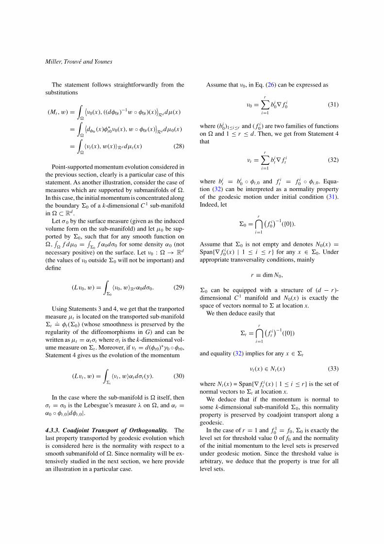
Shown in Fig. 4–6 are examples illustrating the im-age based momentum and the diffeomorphisms gener-ated via geodesic shooting. Figure 4 shows the resultsof the translation experiment. Panels 1 and 2 show I0
and I1; panel 3 shows the diffeomorphism generatedvia geodesic shooting applied to I0, and illustrates howsolving the conservation of momentum equation allowsto recover I1 from I0 and Lv0.
Shown in panel 4 is the density α showing theconcentration near the boundary of I0. Superposed in
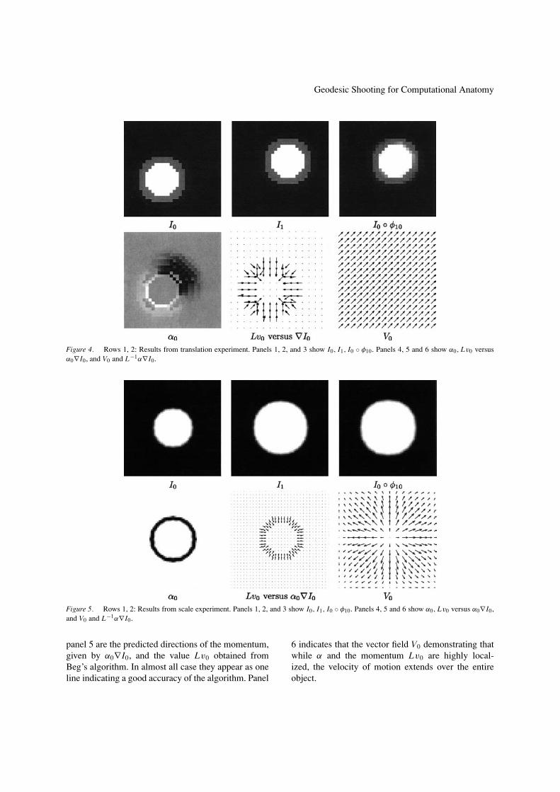
Geodesic Shooting for Computational Anatomy
Figure 4. Rows 1, 2: Results from translation experiment. Panels 1, 2, and 3 show I0, I1, I0 ◦ φ10. Panels 4, 5 and 6 show α0, Lv0 versusα0∇ I0, and V0 and L−1α∇ I0.
Figure 5. Rows 1, 2: Results from scale experiment. Panels 1, 2, and 3 show I0, I1, I0 ◦ φ10. Panels 4, 5 and 6 show α0, Lv0 versus α0∇ I0,and V0 and L−1α∇ I0.
panel 5 are the predicted directions of the momentum,given by α0∇ I0, and the value Lv0 obtained fromBeg’s algorithm. In almost all case they appear as oneline indicating a good accuracy of the algorithm. Panel
6 indicates that the vector field V0 demonstrating thatwhile α and the momentum Lv0 are highly local-ized, the velocity of motion extends over the entireobject.

Miller, Trouve and Younes
Figure 6. Results from mitochondria 2. Panels 1, 2, and 3 show I1, I0, I1 ◦ φ10. Panels 4, 5 and 6 show α0, LV0 versus α0∇ I0, and V0.
Shown in Fig. 5 are similar results for the scaleexperiment.
Shown in Fig. 6 are two sets of results for thegeodesic shooting of the mitochondria. The organi-zation of the results are the same as for the translationand scale experiments. Shown in Fig. 6 are two sets ofresults for the geodesic shooting of the mitochondria.The organization of the results are the same as for thetranslation and scale experiments.
Appendix A: Proof of Theorem 3
Proof: Since g⊥It
is closed, we have to show that foralmost all t, vt = pIt (vt ). Denote ht
.= vt − pIt (vt ).For ε ∈ [0, 1], let vε
t.= vt + εht , and φε
t.= φvε
t (onecan check, but we skip the argument, that t → ht ismeasurable and belongs to L2([0, 1], g), so that thisvariation is valid).
The proof essentially consists in showing that, forall 0 ≤ t ≤ 1
I0 ◦ φt0 = I0 ◦ φεt0. (51)
Indeed, assume that this result is proved. Consider-ing ε = 1 and t = 1, we deduce that I1 = I0 ◦ φ1
1,0.However, since 〈ht , vt 〉L = 〈vt − pIt (vt ), vt 〉L = 0,we get |vt + ht |2L = |vt |2L − |ht |2L . Since t → vt cor-responds to paths with lowest kinetic energy from I0
to I1, we deduce that∫ 1
0 |ht |2L dt = 0 and the proof isended.
We now return to Eq. (51). Using the formula
dφt0(x)
dt= −dxφt0vt (x)
and letting qεt (x) = φt0 ◦ φε
0t (x), we obtain
∂qεt (x)
∂t= −dφε
0t (x)φt0vt ◦ φε0t (x)
+dφε0t (x)φt0
(vt ◦ φε
0t (x) + εht ◦ φε0t (x)
)
= εdφε0t (x)φt0ht ◦ φε
0t (x)
We first prove Eq. (51) under the assumption that I0 isC1. From the computation above, we have
∂
∂t
(I0 ◦ qε
t
)(x) = ε
⟨∇φt0(φε0t (x))
I0, dφε0t (x)φt0ht ◦ φε
0t (x)⟩Rd
= ε⟨∇φε
0t (x) It , ht (φεt0(x)))
⟩Rd = 0
since by definition of the projection pIt (vt ), we havefor any x ∈ �
〈ht (x),∇ It (x)〉Rd = 〈vt (x),
∇ It (x)〉Rd − 〈pIt (vt ),∇ It (x)〉Rd = 0.

Geodesic Shooting for Computational Anatomy
Figure 7. Results from mitochondria 1. Panels 1, 2, and 3 show I0, I1, I0 ◦ φ10. Panels 4, 5 and 6 show α0, LV0 versus α0∇ I0, and V0.
This implies I0 ◦ φt,0 ◦ φε0,t = I0 which yields Eq.
(51) in this case. When I0 is not smooth, the proof goesby showing that
∂
∂t
∫
�
I0 ◦ qεt (x) f (x)dx =
∫
�
It (x) div(ht g
εt
)(x)dx
for smooth f on � and gεt ◦ φε
t |dφεt | = f which can
be done either by a direct (heavy) computation, or byusing a density argument, based on the fact that, by thedivergence theorem, this is true for smooth I0 (we skipthe details). �
Notes
1. These arguments are purely formal since ht includes the Liebracket which cannot be guaranteed to belong to g (in which caseour variation would not be justified).
2. When I has smooth level sets, we say that a vector field ν isnormal to its level sets when, denoting by �i the set {I ≤ i}, v(x)is normal to ∂�i if x ∈ ∂�i for some i and x = 0 otherwise.
3. The explicit form for L−1 depending on the kernel K is definedas follows. For any x, y ∈ �, the bilinear form Kx,y on R
d × Rd
defined by
Kxy (a, b).= 〈δ∗
x a, δ∗y b〉g∗ = (δ∗
y b, L−1(δ∗x a))
= 〈L−1(δ∗x a)(y), b〉
Rd (49)
Acknowledgments
Michael I. Miller was supported by grants from theNational Institute of Wealth numbers P41-RR15241-01A1, U24-RR0211382-01, P20-MH071616-01.
References
1. V.I. Arnold, Mathematical Methods of Classical Mechanics,Springer, 1989. 1st edition 1978.
2. V. Arnold and B. Khesin, “Topological methods in hydrody-namics” Ann. Rev. Fluid Mech., Vol. 24, pp. 145–166, 1992.
3. V.I. Arnold, “Sur la geometrie differentielle des groupes de Liede dimension infinie et ses applications a l’hydrodynamiquedes fluides parfaits,” Ann. Inst. Fourier (Grenoble), Vol. 1, pp.319–361, 1966.
4. M.F. Beg, M.I. Miller, A. Trouve, and L. Younes, “Computinglarge deformation metric mappings via geodesics flows of dif-feomorphisms,” Int. J. Comp. Vis., Vol. 61, No. 2, pp. 139–157,February 2005.
5. V. Camion and L. Younes, “Geodesic interpolating splines,”in M.A.T. Figueiredo, J. Zerubia, and A.K. Jain (Eds.), EMM-CVPR 2001, Vol. 2134 of Lecture Notes in Computer Sciences,Springer-Verlag, 2001, pp. 513–527.
6. T. Chen and D. Metaxas, “Image segmentation based onthe integration of Markov random fields and deformablemodels,” in Medical Image Computing and Computer-Assisted Intervention—Miccai 2000, Vol. 1935 of LectureNotes in Computer Science, Springer-Verlag, 2000, pp. 256–265.

Miller, Trouve and Younes
7. G.E. Christensen, R.D. Rabbitt, and M.I. Miller, “Deformabletemplates using large deformation kinematics,” IEEE Trans.Image Processing, Vol. 5, No. 10, pp. 1435–1447, 1996.
8. I. Cohen, L. Cohen, and N. Ayache, “Using deformable surfacesto segment 3-d images and infer differential structures,” Com-puter Vision Graphics Image Processing, Vol. 56, No. 2, pp.242–263, 1992.
9. T. Cootes, C. Taylor, D. Cooper, and J. Graham, “Active shapemodels—Their training and application,” Comp. Vision and Im-age Understanding, Vol. 61, No. 1, pp. 38–59, 1995.
10. M C. Delfour, and J.-P. Zolesio, Shapes and Geometries. Anal-ysis, Differential Calculus and Optimization, SIAM, 2001.
11. P. Dupuis, U. Grenander, and M. Miller, “Variational problemson flows of diffeomorphisms for image matching,” Quart. App.Math., Vol. 56, pp. 587–600, 1998.
12. A. Garrido and N.P. De la Blanca, “Physically-based activeshape models: Initialization and optimization,” Pattern Recog-nition, Vol. 31, No. 8, pp. 1003–1017, 1998.
13. U. Grenander, General Pattern Theory. Oxford Univeristy Press,1994.
14. U. Grenander, Y. Chow, and D. Keenan, HANDS: A Pattern The-oretic Study of Biological Shapes. Springer-Verlag: New York,1990.
15. U. Grenander and M.I. Miller, “Representations of knowledgein complex systems,” J. Roy. Stat. Soc. B, Vol. 56, No. 3, pp.549–603, 1994.
16. U. Grenander and M.I. Miller, “Computational anatomy: Anemerging discipline,” Quart. App. Math., Vol. 56, pp. 617–694,1998.
17. S. Joshi and M.I. Miller, “Landmark matching via large de-formation diffeomorphisms,” IEEE Trans. Image Processing,Vol. 9, No. 8, pp. 1357–1370, 2000.
18. M. Kass, A. Witkin, and D. Terzopolous, “Snakes: Active con-tour models,” International Journal of Computer Vision, Vol. 1,No. 4, pp. 321–331, 1988.
19. J.E. Marsden, and T.S. Ratiu, Introduction to Mechanics andSymmetry. Springer, 1994.
20. M. Mignotte and J. Meunier, “A multiscale optimization ap-proach for the dynamic contour-based boundary detection is-sue,” Computerized Medical Imaging and Graphics, Vol. 25,No. 3, pp. 265–275, 2001.
21. M. Miller, S. Joshi, D.R. Maffitt, J.G. McNally, and U. Grenan-der, “Mitochondria, membranes and amoebae: 1, 2 and 3 di-mensional shape models,” in Statistics and Imaging, K. Mardia,(Ed.), Vol. II. Carfax Publishing: Abingdon, Oxon., 1994.
22. M. Miller, A. Trouve, and L. Younes, “On the metrics and Euler-Lagrange equations of computational anatomy,” Annual Reviewof Biomedical Engineering, Vol. 4, pp. 375–405, 2002.
23. M. Miller and L. Younes, “Group actions, homeomorphisms,and matching: A general framework,” International Journal ofComputer Vision, Vol. 41(No. 1/2): pp. 61–84, 2001.
24. J. Montagnat and H. Delingette “Volumetric medical imagessegmentation using shape constrained deformable models,” inCvrmed-Mrcas’97, Vol. 1205 of Lecture Notes in ComputerScience, Springer-Verlag, 1997, pp. 13–22.
25. J. Montagnat, H. Delingette, and N. Ayache, “A review of de-formable surfaces: Topology, geometry and deformation,” Im-age and Vision Computing, Vol. 19, No. 14, pp. 1023–1040,2001.
26. D. Mumford, “Pattern theory and vision,” in QuestionsMathematiques En Traitement Du Signal et de L’Image, InstitutHenri Poincare, 1998, Chap. 3, pp. 7–13.
27. S. Osher and J.A. Sethian, “Front propagating with curva-ture dependent speeds: Algorithms based on Hamilton-Jacobiformulation,” Journal of Comp. Physics, Vol. 79, pp. 12–49,1988.
28. D. Pham, C. Xu, and J. Prince, “Current methods in medicalimage segmentation,” Ann. Rev. Biomed. Engng., Vol. 2, pp.315–337, 2000.
29. N. Schultz and K. Conradsen, “2d vector-cycle defonnable tem-plates,” Signal Processing, Vol. 71, No. 2, pp. 141–153, 1998.
30. S. Sclaroff and L.F. Liu, “Deformable shape detection and de-scription via model-based region grouping,” IEEE Transactionson Pattern Analysis and Machine Intelligence, Vol. 23, No. 5,pp. 475–489, 2001.
31. L. Staib and J. Duncan, “Boundary finding with parametricallydeformable models,” IEEE Trans. Pattern Analysis and MachineIntelligence, Vol. 14, pp. 1061–1075, 1992.
32. L. Staib and J. Duncan, “Model-based deformable surface find-ing for medical images,” IEEE Trans. Medical Imaging, Vol. 15,No. 5, pp. 1–13, 1996.
33. D. Terzopoulos and D. Metaxas, “Dynamic models with lo-cal and global deformations: Deformable superquadrics,” IEEETrans. Patt. Anal. Mach. Intell., Vol. 13, pp. 703–714, 1991.
34. A. Trouve and L. Younes, “Local geometry of deformable tem-plate,” SIAM Journal of Mathmatical Analysis (to appear).
35. A. Trouve, “Action de groupe de dimension infinie et reconnais-sance de formes. C.R. Acad. Sci. Paris, Serie I, No. 321, pp.1031–1034, 1995.
36. A. Trouve, “Diffeomorphisms groups and pattern matching inimage analysis,” Int. J. Computer Vision, Vol. 28, pp. 213–221,1998.
37. M. Vaillant and C. Davatzikos, “Finding parametric represen-tations of the cortical sulci using an active contour model,”Medical Image Analysis, Vol. 1, No. 4, pp. 295–315, 1997.
38. C.F. Westin, L.M. Lorigo, O. Faugeras, W.E.L. Grimson, S.Dawson, A. Norbash, and R. Kikinis, “Segmentation by adaptivegeodesic active contours,” in Medical Image Computing andComputer-Assisted Intervention—MICCAI 2000, Vol. 1935 ofLecture Notes in Computer Science, Springer-Verlag, 2000, pp.266–275.
39. C. Xu, D.L. Pham, and J.L. Prince, “Finding the brain cortexusing fuzzy segmentation, isosurfaces and deformable surfacemodels,” in XVth Int. Conf. on info Proc. in Medical Imaging,June 1997.
40. C. Xu, D.L. Pham, and J.L. Prince, “Medical image segmenta-tion using deformable models,” in SPIE Handbook on MedicalImaging - Volume III: Medical Image Analysis, J. Fitzpatrick andM. Sonka, (Eds.) SPIE, Bellingham, WA, 2000, pp. 129–174.
41. C. Xu and J.L. Prince, “Gradient vector flow: A new externalforce for snakes,” CVRP, Nov. 1997.
42. C. Xu and J.L. Prince, “Gradient vector flow deformable mod-els,” in Handbook of Medical Imaging, I. Bankman, (Ed.), Aca-demic Press: San Diego, CA, 2000.
43. A. Yezzi, A. Tsai, and A. Willsky, “A fully global approachto image segmentation via coupled curve evolution equations,”Journal of Visual Communication and Image Representation,Vol. 13, No. 1–2, pp. 195–216, 2002.