Observing geomagnetic induction in magneticsatellite measurements and associatedimplications for mantle conductivity

Steven Constable and Catherine ConstableInstitute of Geophysics and Planetary Physics, Scripps Institution of Oceanography, La Jolla, California 92093, USA(sconstable@ucsd.edu; cconstable@ucsd.edu)

[1] Currents induced in Earth by temporal variations in the external magnetic field have long been used to

probe mantle electrical conductivity, but almost exclusively from sparsely distributed land observatories.

Satellite-borne magnetometers, such as flown on Magsat, Ørsted, and Champ, offer the prospect of

improved spatial coverage. The approach we have taken is to isolate induction by harmonic Dst

(‘‘disturbance storm time’’) excitation of the magnetospheric ring current in satellite magnetic

measurements: this is done by removing the magnetic contributions of the main (core) magnetic field,

the crustal magnetic field, and ionospheric fields (cause of the daily variation) using Sabaka et al.’s [2000,

2002] CMP3 comprehensive model. The Dst signal is then clearly evident in the midlatitude satellite

passes lower than 50 degrees geomagnetic latitude. At higher latitudes, auroral and field aligned currents

contaminate the data. We fit the internal and external components of the Dst signal for each equatorial pass,

exploiting the fact that the geometry for the internal and external components is different for the azimuthal

and radial vector components. The resulting timeseries of internal and external field variations shows that

the Dst signals for the dawn passes are half those of the dusk passes. The sum of equatorial external and

internal components of the field averaged over dawn and dusk passes provides an excellent estimate for the

Dst index, and may in fact be superior when used as a proxy for the purposes of removing induced and

magnetospheric fields from satellite magnetic data. We call this estimate satellite Dst. Cross spectral

analysis of the internal and external timeseries shows both greater power and higher coherence in the dusk

data. We processed the transfer function between internal and external dusk timeseries to provide globally-

averaged, frequency dependent impedances that agree well with independently derived estimates. We

estimate Earth’s radial electrical conductivity structure from these impedances using standard regularized

inversion techniques. A near-surface conductor is required, of thickness less than 10 km with a

conductivity-thickness product almost exactly that of an average Earth ocean. Inversions suggest that an

increase in conductivity at 440 km depth, predicted by recent laboratory measurements on high pressure

phases of olivine, is not favored by the data, although, as in previous studies, the 670 km discontinuity

between the upper and lower mantle is associated with a two orders of magnitude jump in conductivity. A

new feature in our inversions is a further increase in lower mantle conductivity at a depth of 1300 km. A

global map of the internal (induced) component of the magnetic field provides a qualitative estimate of

three-dimensional (3-D) variations in Earth electrical conductivity, demonstrating graphically that the

satellite data are responsive to lateral variations in electrical conductivity caused by the continents and

oceans.

Components: 3786 words, 11 figures, 2 tables.

Keywords: Satellite induction.

Index Terms: 1515 Geomagnetism and Paleomagnetism: Geomagnetic induction; 3914 Mineral Physics: Electrical

G3G3GeochemistryGeophysics

Geosystems

Published by AGU and the Geochemical Society

AN ELECTRONIC JOURNAL OF THE EARTH SCIENCES

GeochemistryGeophysics

Geosystems

Article

Volume 5, Number 1

20 January 2004

Q01006, doi:10.1029/2003GC000634

ISSN: 1525-2027

Copyright 2004 by the American Geophysical Union 1 of 15

properties; 1555 Geomagnetism and Paleomagnetism: Time variations—diurnal to secular.

Received 15 September 2003; Revised 21 November 2003; Accepted 1 December 2003; Published 20 January 2004.

Constable, S., and C. Constable (2004), Observing geomagnetic induction in magnetic satellite measurements and associated

implications for mantle conductivity, Geochem. Geophys. Geosyst., 5, Q01006, doi:10.1029/2003GC000634.

1. Introduction

[2] Schuster [1889] was first to note inductive

effects associated with the daily variations of

Earth’s magnetic field. Since that time an industry

has developed whereby currents induced in Earth

by temporal variations in the external magnetic

field have been used to probe mantle electrical

conductivity [e.g., Lahiri and Price, 1939; Banks,

1969; Schultz and Larsen, 1987, 1990; Constable,

1993; Olsen, 1999a], but generally from sparsely

distributed land observatories. Satellite-borne mag-

netometers, such as flown on Magsat, Ørsted, and

Champ, offer the prospect of improved spatial

coverage. However, the task of separating the

temporal and spatial signals, mixed together as

the satellite passes over regions of variable electri-

cal conductivity while the external magnetic field

varies in intensity and direction, is by no means

trivial, and only a few authors have tackled this

problem [e.g., Didwall, 1984; Oraevsky et al.,

1993; Olsen, 1999b]. Their efforts are thoroughly

reviewed by Olsen [1999b], who noted that the

shorter time series of satellite data tended to

produce noisier results than ground data. In his

new analysis of Magsat data, Olsen [1999b] found

higher resistivity in oceanic than continental areas,

but because of a lack of frequency dependence in

the results he attributes at least part of this differ-

ence to causes other than mantle conductivity.

[3] In this paper we derive estimates of conduc-

tivity from frequency dependent impedance re-

sponse functions generated from the ratio of

internal to external parts of the geomagnetic field.

The external source field we consider is that

generated by Dst (‘‘ring current’’) variations, over

periods ranging from about 7 hours to 100 days.

We use vector field data from Magsat and Sabaka

et al.’s [2000] comprehensive magnetic field

model to remove non-inductive components from

the magnetic field data (i.e., crustal and main field

signals) and ionospheric contributions (the daily

variation). We generate complete time series of

the inductive component (instead of selecting only

energetic storm-time events), use modern, robust

multitaper time series analysis, modern one-

dimensional (1-D) regularized inversion studies,

and generate qualitative global images of geo-

magnetic induction in Earth.

[4] The ultimate goal of this study is to image

one-dimensional and three-dimensional electrical

conductivity structure of Earth’s mantle. One

dimensional (1-D) structure is influenced most

by pressure dependent phase changes, and prob-

ably represents the dominant conductivity signal

within the mantle and core. Three dimensional

(3-D) structure can provide information about

lateral variations in temperature and trace vola-

tiles in the mantle. In the crust, 3-D structure

dominates the conductivity signal, reflecting the

large lateral changes found in the temperature,

porosity, and water content of crustal rocks, as

well as the ocean/continent signal.

2. Dst and the Ring Current

[5] Banks [1969] showed that variations in Earth’s

magnetic field at periods shorter than one year are

dominated by a simple P10 spherical harmonic

geometry. Later work confirms this, and deter-

mines the cause to be the excitation of the

equatorial ring current, a westward propagating

current between 2 and 9 Earth radii that is

populated with charge carriers, mainly oxygen

ions from the upper atmosphere, during magnetic

storms driven by the solar wind (see the review

by Daglis et al. [1999]). During quiescent times

the ring current is populated mainly by protons.

Excitation of the ring current serves to oppose

Earth’s main field at the equator, and so produces

GeochemistryGeophysicsGeosystems G3G3

constable and constable: satellite induction 10.1029/2003GC000634

2 of 15

a magnetic field aligned with main field at the

poles (vertically down at the north pole).

[6] The strength of the ring current is character-

ized by the ‘‘Dst’’ (disturbance storm time) index,

an index of magnetic activity derived from a

network of low to midlatitude geomagnetic

observatories that measures the intensity of the

globally symmetrical part of the equatorial ring

current. An early method for derivation of the Dst

index is described in Sugiura [1964], the current

method is updated in IAGA Bulletin No. 40, a

report by Masahisa Sugiura which presents the

values of the equatorial Dst index for 1957–1986.

This can be found on the Web at http://

swdcdb.kugi.kyoto-u.ac.jp/dst2/onDstindex.html.

Honolulu, Hermanus, San Juan and Kakioka are

the current contributing observatories. During the

Magsat mission, Alibag provided supplemental

longitudinal coverage.

[7] The actual morphology of the ring current fields

is asymmetric about the day/night hemispheres

[Chapman and Bartels, 1940], and strictly speaking

one should preserve a distinction between Dst, the

index, and the actual ring current fields, but we relax

this distinction here for the sake of readability.

3. Isolating Dst From SatelliteObservations

[8] Magsat flew fromNovember 1979 toMay 1980,

and collected both vector and scalar magnetic field

data in a sun-synchronous orbit. That is, the satellite

passed from local solar dawn (06:00) to local solar

dusk (18:00) during every orbit. Magsat’s altitude

ranged from 325–550 km. Vector fluxgate magne-

tometer data (approximate accuracy 6 nT) decimated

to 0.1 Hz were used (M. Purucker, personal com-

munication), and we rejected all measurements with

attitude flag �7000. We used the Comprehensive

Model of the Near-Earth Magnetic Field: Phase 3

[Sabaka et al., 2000]. This model, designated

CMP3, includes estimates of the following: The

main (core) field, and its secular variation, the

crustal (lithospheric) field due to remanent and

induced magnetization, ionospheric currents (daily

and storm-time variations), field aligned and merid-

ional currents, and seasonal variations, equatorial

electrojet, magnetospheric ring current, and cou-

pling and induction of the above. (A later version

of the Comprehensive Model, designated CM3

[Sabaka et al., 2002], was made available during

the course of this work. We tested this version of

the model and concluded that CMP3 did a slightly

better job of fitting the Magsat data set than did

CM3, and so kept our original analysis.)

[9] Parameters supplied to CMP3 for every data

point are position in geomagnetic coordinates,

magnetic universal time [Sabaka et al., 2000],

and insolation represented by the 10.7 cm radio

flux. The ring current and storm-time variations are

modeled via a dependence on the Dst index. We

turned off this part of the model by setting Dst = 0

and use the residuals after predicting the vector

Magsat data with CMP3 as our initial model. We

designate these the ‘‘CMP3-Dst’’ residuals. (A

25 nT static component of the ring current is still

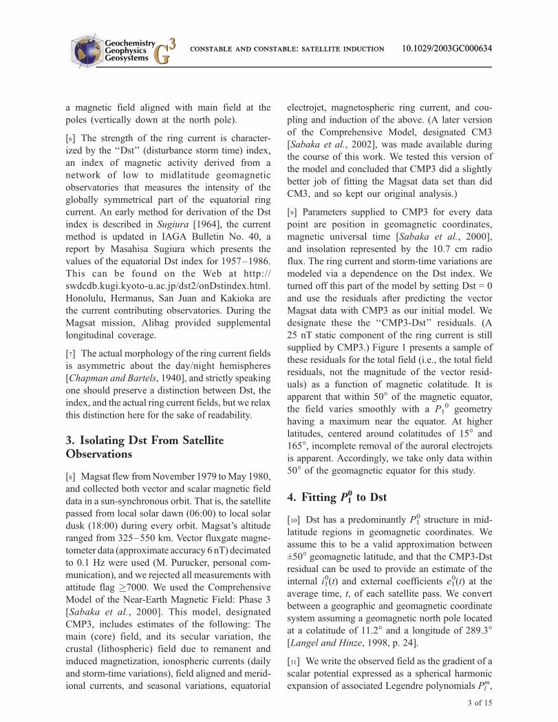
supplied by CMP3.) Figure 1 presents a sample of

these residuals for the total field (i.e., the total field

residuals, not the magnitude of the vector resid-

uals) as a function of magnetic colatitude. It is

apparent that within 50� of the magnetic equator,

the field varies smoothly with a P10 geometry

having a maximum near the equator. At higher

latitudes, centered around colatitudes of 15� and

165�, incomplete removal of the auroral electrojets

is apparent. Accordingly, we take only data within

50� of the geomagnetic equator for this study.

4. Fitting P10 to Dst

[10] Dst has a predominantly P10 structure in mid-

latitude regions in geomagnetic coordinates. We

assume this to be a valid approximation between

±50� geomagnetic latitude, and that the CMP3-Dst

residual can be used to provide an estimate of the

internal i10(t) and external coefficients e1

0(t) at the

average time, t, of each satellite pass. We convert

between a geographic and geomagnetic coordinate

system assuming a geomagnetic north pole located

at a colatitude of 11.2� and a longitude of 289.3�[Langel and Hinze, 1998, p. 24].

[11] We write the observed field as the gradient of a

scalar potential expressed as a spherical harmonic

expansion of associated Legendre polynomials Plm,

GeochemistryGeophysicsGeosystems G3G3

constable and constable: satellite induction 10.1029/2003GC000634constable and constable: satellite induction 10.1029/2003GC000634

3 of 15

with Schmidt quasi-normalized spherical harmonic

coefficients representing the internal ilm(t) and

external elm(t) magnetic fields:

� r; q;fð Þ ¼ aoX1l¼1

Xl

m¼�l

iml tð Þ ao

r

� �lþ1�

þ eml tð Þ r

ao

� �l)Pml cos qð Þeimf:

Keeping only the P10 contribution and with r, q, f

in geomagnetic coordinates

�01 r; qð Þ ¼ ao i01 tð Þ ao

r

� �2�

þ e01 tð Þ r

ao

� ��P01 cos qð Þ

and so the magnetic induction B is derived from

the negative of the gradient in the usual manner

B r; q;fð Þ ¼ �r�01 r; q;fð Þ

or, expressed as components Br, Bq, Bf of a

spherical coordinate system:

Br ¼ �e01 þ 2i01a

r

� �3

cos qð Þ

Bq ¼ e01 þ i01a

r

� �3

sin qð Þ

Bf ¼ 0:

The above, neglecting the azimuthal (f) compo-

nent (which should be zero), may be expressed in

matrix form as:

� cos qð Þ 2a

r

� �3

cos qð Þ

sin qð Þ a

r

� �3

sin qð Þ

2664

3775

e01

i01

24

35 ¼

Br

Bq

24

35:

[12] Our primary data set is Magsat measurements

re-sampled at 10 s period, and so for a single

30 minute satellite pass between ±50�, we have

typically 100–200 data with different values of

altitude (r) and geomagnetic colatitude (q). We

thus use an overdetermined linear least squares

estimate to evaluate the internal and external

coefficients for each satellite pass. We treat dawn

and dusk passes separately to accommodate the

asymmetry in the ring current structure, which

results in different amplitudes for the Dst field in

the dusk (ascending) and dawn (descending)

passes. Application of least squares estimation to

each pass provides an estimate of i10(t) and e1

0(t) at

about 100 minute intervals for 2762 dawn and

2717 dusk orbits. Figures 2a and 2b show exam-

Figure 1. A sample of CMP3-Dst residuals (the first 100,000 data points) for the total magnetic field plotted asfunction of geomagnetic colatitude, qd. We use only observations in colatitude range 40� < qd < 140� for our modelingto avoid magnetic fields associated with field-aligned currents, here evident as rapidly varying fields peaking within20� of the poles.

GeochemistryGeophysicsGeosystems G3G3

constable and constable: satellite induction 10.1029/2003GC000634

4 of 15

ples of fits to data from two individual passes of

the satellite. The model fits are determined by

only two free parameters for each pass, ilm(t) and

elm(t), with the altitude and magnetic colatitude as

fixed data parameters.

[13] It can be seen from Figure 2 that while our fits

are quite good, particularly considering that we

have only two free parameters, e10(t) and i1

0(t), for

each pass, they are far from perfect. There are

many potential sources of error; the existence of

non-P10 components of the external field, an im-

perfectly removed crustal magnetic field, variations

in electrical conductivity along the satellite pass,

and so on. As one would expect from errors of

these types, the residuals have a strong covariance,

exhibited as a serial correlation in the misfits, and

so one cannot use standard techniques to estimate

the linear errors in the estimates of the coefficients.

We can, however, compare the residuals after our

fitting procedure to those achieved by CMP3 with

the Dst correction turned on. We should naturally

expect a smaller misfit from our procedure, since it

fits the data on a pass by pass basis, while CMP3

uses a global correction for temporal variations in

Dst strength via the Dst index. In many case this

global correction performs well, see, for example,

Figure 2d, but in other cases (Figure 2c) it doesn’t

do such a good job (demonstrating that we are not

simply recovering the Dst index/signal we omitted

from the comprehensive model). In this example,

there is a large asymmetry in the fitted P10 values

between dawn and dusk passes, and while the

average of the two agrees fairly well with obser-

vatory Dst, the assumption of a symmetric ring

current is clearly breaking down.

[14] Table 1 provides a statistical summary of our

fitting. Our signal-to-noise ratio is fairly good,

particularly for Bq where it is three or more on

average, and much larger during storm times. As

expected, our pass by pass fits do a much better job

than the comprehensive model with the Dst cor-

rection turned on. However, by design, the CMP3

model is constructed based on quiet time variations

in the magnetic field (Dst < 20 nT), and Sabaka et

al. [2002] report RMS misfits of little more than 4

nT for this data subset.

Figure 2. Data, fits, and residuals for two dusk passes. (a, b) Blue represents data (asterisk symbols) and fits (solidlines) to the Br component and red represents data and fits for the Bq component. (c, d) Residuals from these fits areagain as shown as colored asterisk symbols. Also shown in the bottom panels are the CMP3 residuals (with the Dstcorrection turned on) for Br and Bq as blue and red circles symbols respectively. For pass number 331 (right), theCMP3 model does a good job of fitting the storm-time fields, but for pass 314 (left), CMP3 does poorly, as is evidentby the large Bq residuals. Satellite altitude is shown in green in Figures 2c and 2d.

GeochemistryGeophysicsGeosystems G3G3

constable and constable: satellite induction 10.1029/2003GC000634

5 of 15

[15] Plots of i10(t) and e1

0(t) for dawn and dusk

passes are presented in Figure 3. It is immediately

apparent that dusk passes are about twice the

magnitude of dawn passes, indicating the asym-

metry in the ring current morphology. However,

the ratio between internal and external fields,

about 0.3, is preserved in both time series. This

ratio of internal to external fields agrees with

value of 0.27 determined by Langel and Estes

[1985] and also used by Olsen et al. [2000] for

the Ørsted initial field model. However, this ratio

is frequency-dependent, which we consider below

in computing transfer functions between internal

and external fields.

5. Replicating Dst

[16] In this section we compare our satellite esti-

mates of the Dst signal strength with those derived

from magnetic observatories. Data from low to

mid-latitude observatories are used for the Dst

index to minimize the influence of both sub-auroral

and equatorial electrojets. Hourly H-component

magnetic variations are analyzed to remove both

the main field baseline and typical quiet-day var-

iations. A cosine factor of the site latitude trans-

forms residual variations to their horizontal field

equatorial equivalents. Results from a number of

observatories are averaged together. The baseline

for Dst is set so that on the internationally desig-

nated 5 quietest days the Dst index is zero on

average. Langel et al. [1980] estimated from Mag-

sat data that the axially symmetric external field

was �25 nT when Dst is zero, and this offset is

Table 1. RMS Residuals From all Dusk and DawnPassesa

Dusk Dawn

X CMP3-Dst 22.9 15.6X CMP3 19.2 12.4Bq This study 6.0 5.2Y CMP3 12.0 9.4Z CMP3-Dst 7.4 6.1Z CMP3 6.5 5.6Br This study 5.2 5.1N 264391 331977

a‘‘This study’’ represents residuals from fitting our model to the

CMP3-Dst data set. For comparison with our CMP3-Dst data set,‘‘CMP3’’ designates residuals obtained running the comprehensivemodel with the Dst correction turned on. ‘‘N’’ is simply the number ofdata supplying the statistics. Note that the results for our study arerotated into geomagnetic coordinates, while the other data are ingeographic coordinates.

Figure 3. Least squares estimates of i10(t) (blue) and e1

0(t) (red) from CMP3-Dst residuals. The upper plot is for duskpasses, lower for dawn.

GeochemistryGeophysicsGeosystems G3G3

constable and constable: satellite induction 10.1029/2003GC000634

6 of 15

modeled by CMP3. However, the Dst offset may

vary with solar cycle.

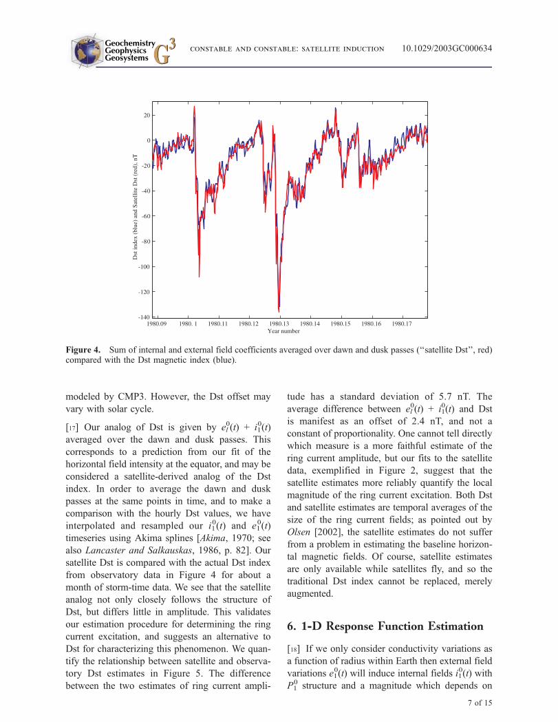
[17] Our analog of Dst is given by el0(t) + i1

0(t)

averaged over the dawn and dusk passes. This

corresponds to a prediction from our fit of the

horizontal field intensity at the equator, and may be

considered a satellite-derived analog of the Dst

index. In order to average the dawn and dusk

passes at the same points in time, and to make a

comparison with the hourly Dst values, we have

interpolated and resampled our i10(t) and e1

0(t)

timeseries using Akima splines [Akima, 1970; see

also Lancaster and Salkauskas, 1986, p. 82]. Our

satellite Dst is compared with the actual Dst index

from observatory data in Figure 4 for about a

month of storm-time data. We see that the satellite

analog not only closely follows the structure of

Dst, but differs little in amplitude. This validates

our estimation procedure for determining the ring

current excitation, and suggests an alternative to

Dst for characterizing this phenomenon. We quan-

tify the relationship between satellite and observa-

tory Dst estimates in Figure 5. The difference

between the two estimates of ring current ampli-

tude has a standard deviation of 5.7 nT. The

average difference between el0(t) + i1

0(t) and Dst

is manifest as an offset of 2.4 nT, and not a

constant of proportionality. One cannot tell directly

which measure is a more faithful estimate of the

ring current amplitude, but our fits to the satellite

data, exemplified in Figure 2, suggest that the

satellite estimates more reliably quantify the local

magnitude of the ring current excitation. Both Dst

and satellite estimates are temporal averages of the

size of the ring current fields; as pointed out by

Olsen [2002], the satellite estimates do not suffer

from a problem in estimating the baseline horizon-

tal magnetic fields. Of course, satellite estimates

are only available while satellites fly, and so the

traditional Dst index cannot be replaced, merely

augmented.

6. 1--D Response Function Estimation

[18] If we only consider conductivity variations as

a function of radius within Earth then external field

variations e10(t) will induce internal fields i1

0(t) with

P10 structure and a magnitude which depends on

Figure 4. Sum of internal and external field coefficients averaged over dawn and dusk passes (‘‘satellite Dst’’, red)compared with the Dst magnetic index (blue).

GeochemistryGeophysicsGeosystems G3G3

constable and constable: satellite induction 10.1029/2003GC000634

7 of 15

Earth conductivity. The frequency dependent trans-

fer function

Ql fð Þ ¼ il fð Þel fð Þ

may thus be used to infer conductivity structure

within Earth, with higher frequencies corresponding

to shallower induced fields. We use multitaper

cross-spectral estimation [Riedel and Sidorenko,

1995] to evaluate this transfer function, with 20

uniform (as opposed to adaptive) tapers. Figure 6

shows the power spectra of the internal and external

fields for the dawn and dusk passes. The dusk passes

have greater power than the dawn passes at all

frequencies. The lower amplitudes of the dawn

passes allow the harmonics of the daily variation, or

Sq, to be seen, indicating that the ionospheric

contribution has been incompletely removed by the

comprehensive model. Figure 7 shows the coher-

ence spectra between e10(t) and i1

0(t) for the dawn and

dusk passes. Overall, the dusk passes have higher

coherence than dawn passes. Although there are

peaks in the spectra at the harmonics of one day,

these correspond to drops in coherence, presumably

because the ionospheric contributions are below the

satellite and do not separate coherently into internal

and external components.

[19] To evaluate Q1, we average estimates of the

transfer functions using both i10 and e1

0 as inputs to

remove bias associated with noise in the input

time series, which in standard spectral analysis is

assumed to be noise-free. We carry out band

averaging to improve statistical reliability, weight-

ing individual estimates byffiffiffiffiffiffiffiffiffiffiffiffiffi1� g2

p, where g is

coherency, which is a measure of standard devi-

ation in the estimates. To avoid using daily

harmonics and other low-coherence data, we re-

ject data with a coherence-squared less than 0.6.

This is a purely heuristic choice based on exper-

imenting with the trade-off between the number

of data in the band average versus the uncertainty

of the individual estimates used in the average.

The dawn coherency spectrum has very few data

above this cutoff, and results in estimates of Q1

that are clearly biased relative to previous esti-

mates, and so we use only the dusk data in our

estimates of Q1.

Figure 5. Scatterplot of dawn/dusk average of total field estimated from satellite data ([el0(t) + i1

0(t)]/2) against theDst index.

GeochemistryGeophysicsGeosystems G3G3

constable and constable: satellite induction 10.1029/2003GC000634

8 of 15

Figure 6. Spectra of the four timeseries shown in Figure 3. It can be seen that the dusk passes have greater powerthan the dawn passes at all frequencies, and are less contaminated by harmonics of the daily variation.

Figure 7. Coherence spectra between e10(t) and i1

0(t) for the dawn and dusk timeseries. Coherences are higher for thedusk data, but drop at harmonics of one day, presumably because of contamination from ionospheric sources.

GeochemistryGeophysicsGeosystems G3G3

constable and constable: satellite induction 10.1029/2003GC000634

9 of 15

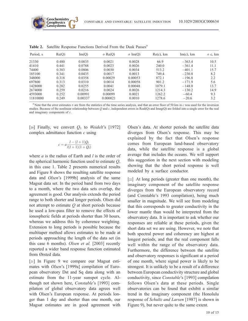
[20] Finally, we convert Q1 to Weidelt’s [1972]

complex admittance function c using

c ¼ al � l þ 1ð ÞQl

l l þ 1ð Þ 1þ Qlð Þ

where a is the radius of Earth and l is the order of

the spherical harmonic function used to estimate Q,

in this case 1. Table 2 presents numerical results

and Figure 8 shows the resulting satellite response

data and Olsen’s [1999b] analysis of the same

Magsat data set. In the period band from two days

to a month, where the two data sets overlap, the

agreement is good. Our analysis extends the period

range to both shorter and longer periods. Olsen did

not attempt to estimate Q at short periods because

he used a low-pass filter to remove the effects of

ionospheric fields at periods shorter than 30 hours,

whereas we address this by coherence weighting.

Extension to long periods is possible because the

multitaper method allows estimates to be made at

periods approaching the length of the data set (in

this case 6 months). Olsen et al. [2003] recently

reported a wider band response function estimated

from Ørsted data.

[21] In Figure 9 we compare our Magsat esti-

mates with Olsen’s [1999a] compilation of Euro-

pean observatory Dst and Sq data along with an

estimate from the 11-year sunspot cycle. Al-

though not shown here, Constable’s [1993] com-

pilation of global observatory data agrees well

with Olsen’s European response. At periods lon-

ger than 1 day and shorter than one month, our

Magsat estimates are in good agreement with

Olsen’s data. At shorter periods the satellite data

diverges from Olsen’s response. This may be

explained by the fact that Olsen’s response

comes from European land-based observatory

data, while the satellite response is a global

average that includes the oceans. We will support

this suggestion in the next section with modeling

showing that the short period response is well

modeled by a surface conductor.

[22] At long periods (greater than one month), the

imaginary component of the satellite response

diverges from the European observatory record

(and Constable’s 1993 compilation), being much

smaller in magnitude. We will see from modeling

that this corresponds to greater conductivity in the

lower mantle than would be interpreted from the

observatory data. It is important to ask whether our

responses are reliable at these periods, given the

short data set we are using. However, we note that

both spectral power and coherency are highest at

longest periods, and that the real component falls

well within the range of the observatory data.

Furthermore, the difference between the satellite

and observatory responses is significant at a period

of one month, where signal power is likely to be

strongest. It is unlikely to be a result of a difference

between European conductivity structure and global

conductivity, since Constable’s [1993] compilation

follows Olsen’s data at these periods. Single

observatories can be found that exhibit a similar

trend in the imaginary component (the Honolulu

response of Schultz and Larsen [1987] is shown in

Figure 9), but never quite to the same extent.

Table 2. Satellite Response Functions Derived From the Dusk Passesa

Period, s Re(Q) Im(Q) s Re(Q) s Im(Q) Re(c), km Im(c), km s c, km

21330 0.480 0.0835 0.0021 0.0028 66.9 �363.4 10.541410 0.441 0.0788 0.0023 0.0026 240.0 �361.4 11.174400 0.383 0.0806 0.0030 0.0034 513.2 �401.1 15.7185100 0.341 0.0435 0.0017 0.0013 749.4 �230.8 8.2348000 0.318 0.0358 0.00029 0.00053 872.1 �196.8 2.2697800 0.313 0.0310 0.0014 0.00058 901.2 �171.9 5.61428000 0.282 0.0255 0.0041 0.00048 1079.1 �148.0 13.72674000 0.259 0.0216 0.0024 0.0026 1214.3 �130.2 14.94593000 0.252 0.00991 0.00099 0.0021 1262.2 �60.4 9.311810000 0.249 0.00337 0.000021 0.0010 1278.6 �20.6 3.2

aNote that the error estimates s are from the statistics of the time series analysis, and that an error floor of 50 km in c was used for the inversion

studies. Because of the nonlinear relationship between Q and c, independent errors in Real(Q) and Imag(Q) are folded into a single error for the realand imaginary components of c.

GeochemistryGeophysicsGeosystems G3G3

constable and constable: satellite induction 10.1029/2003GC000634

10 of 15

Figure 8. 1-D transfer functions from this study (black), and Olsen’s [1999b] study of the same Magsat data set(red). Solid lines show least squares best fitting model responses (D+) for our data.

Figure 9. Our Magsat 1-D response function (black), the European observatory average of Olsen [1999a] (red)which includes the 11 year estimate of Harwood and Malin [1977], and Schultz and Larsen’s [1987] response for theHonolulu observatory (blue).

GeochemistryGeophysicsGeosystems G3G3

constable and constable: satellite induction 10.1029/2003GC000634

11 of 15

[23] One possible explanation for the long period

discrepency lies in the nature of the time series

estimation we have used. Each point in our times-

eries results from a fit of internal and external P10

components to data which span a range of latitudes

and altitudes. Observatory studies either assume a

P10 geometry a priori, or, at best, use a range of

latitudes to do the fitting. It is therefore possible

that the observatory studies are contaminated by

non-P10 magnetic fields at the longer periods. We

suggest this as a tentative hypothesis, further work

will be required to support this idea.

7. 1-D Conductivity Model Estimation

[24] Parker and Whaler’s [1981] D+ algorithm

provides the best possible fit to the data in a least

squares sense for a 1-D Earth structure. Using error

bars estimated from spectral analysis statistics,

D+ fitting provides unacceptable misfits for the

response function. Instead, we assign an error floor

of 50 km to the data, which corresponds to a D+

misfit of RMS 0.95. The response of the D+ model

to these modified data is shown by the solid line in

Figure 8.

[25] Whilst the D+ algorithm provides an estimate

of the best possible fit to a data set, the model

associated with the response function is unphys-

ical, consisting of delta functions of conductivity in

an insulating half-space. For more realistic models,

we use the Occam algorithm of Constable et al.

[1987] [see also Parker, 1994] which generates a

maximally smooth model (measured as the first

derivative of log[conductivity] with respect to

log[depth]) for a given data misfit. We have mod-

ified the implementation of the Occam algorithm in

two ways; we have corrected the 1-D forward

model calculations for spherical Earth geometry

using the method of Weidelt [1972], and we have

terminated the model with a highly conducting

core at a depth of 2886 km.

[26] The one free parameter associated with the

Occam approach is the appropriate misfit level.

With well behaved error statistics and no features

in the data other than those generated by a 1-D

model, statistical arguments can be used to

choose a misfit level, such as an expected value

of RMS = 1. However, we have already used a

more heuristic approach by assigning an error

floor based on D+ fitting. Given this error floor

and by examining smooth models at various

misfit levels, we present a smooth model fitting

the data to RMS 1.15 in Figure 10. The salient

features of this model do not change significantly

as the misfit is increased or decreased a moderate

amount. All models exhibit a large jump from

about 0.01 S/m to about 2 S/m at a depth of

around 700 km. This feature is seen in many

induction studies and is thought to be associated

with the phase transition from garnet and olivine

spinel above 670 km to magnesiowustite and

silicate perovskite below this depth. There is

little evidence for a shallower increase in con-

ductivity at the 440 km phase transition from

olivine to beta spinel as predicted by Xu et al.

[1998]. All models show a further increase in

conductivity at a depth of 1300 km. This feature

is not widely reported in other studies, and is

generated by the small imaginary components of

the response function at long period. It is worth

noting that this model, while incompatible with

Olsen’s [1999a] and Constable’s [1993] observa-

tory compilations, is in fact compatible with the

11-year response of Harwood and Malin [1977].

[27] Both the smooth model and D+ exhibit a region

of increased conductivity near the surface, at depths

less than a few tens of kilometers. This feature is not

seen when inverting the observatory data, and is a

consequence of including the shorter period satellite

response collected over both oceans and continents.

The D+ model includes a surface conductance of

8300 S, which is nicely explained by an ocean depth

of 2800 km (averaged over seas and continents) and

the conductivity of seawater (3 S/m).

[28] The upper mantle conductivity agrees well

with a temperature of around 1400�C and the

SO2 conductivity-temperature relationship for dry

olivine developed by Constable et al. [1992]. This

is further supported by an estimated 1400�C tem-

perature for the 440 km transition from olivine to

spinel [Katsura et al., 1998; Akaogi et al., 1989].

However, the conductance, or conductivity-thick-

ness product, of the average ocean is slightly

greater than the conductance of the mantle part of

GeochemistryGeophysicsGeosystems G3G3

constable and constable: satellite induction 10.1029/2003GC000634

12 of 15

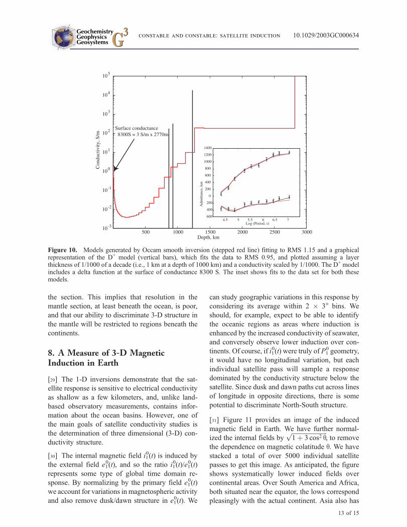
the section. This implies that resolution in the

mantle section, at least beneath the ocean, is poor,

and that our ability to discriminate 3-D structure in

the mantle will be restricted to regions beneath the

continents.

8. A Measure of 3-D MagneticInduction in Earth

[29] The 1-D inversions demonstrate that the sat-

ellite response is sensitive to electrical conductivity

as shallow as a few kilometers, and, unlike land-

based observatory measurements, contains infor-

mation about the ocean basins. However, one of

the main goals of satellite conductivity studies is

the determination of three dimensional (3-D) con-

ductivity structure.

[30] The internal magnetic field i10(t) is induced by

the external field e10(t), and so the ratio i1

0(t)/e10(t)

represents some type of global time domain re-

sponse. By normalizing by the primary field e10(t)

we account for variations in magnetospheric activity

and also remove dusk/dawn structure in e10(t). We

can study geographic variations in this response by

considering its average within 2 3� bins. We

should, for example, expect to be able to identify

the oceanic regions as areas where induction is

enhanced by the increased conductivity of seawater,

and conversely observe lower induction over con-

tinents. Of course, if i10(t) were truly of P1

0 geometry,

it would have no longitudinal variation, but each

individual satellite pass will sample a response

dominated by the conductivity structure below the

satellite. Since dusk and dawn paths cut across lines

of longitude in opposite directions, there is some

potential to discriminate North-South structure.

[31] Figure 11 provides an image of the induced

magnetic field in Earth. We have further normal-

ized the internal fields byffiffiffiffiffiffiffiffiffiffiffiffiffiffiffiffiffiffiffiffiffiffiffi1þ 3 cos2 q

p, to remove

the dependence on magnetic colatitude q. We have

stacked a total of over 5000 individual satellite

passes to get this image. As anticipated, the figure

shows systematically lower induced fields over

continental areas. Over South America and Africa,

both situated near the equator, the lows correspond

pleasingly with the actual continent. Asia also has

Figure 10. Models generated by Occam smooth inversion (stepped red line) fitting to RMS 1.15 and a graphicalrepresentation of the D+ model (vertical bars), which fits the data to RMS 0.95, and plotted assuming a layerthickness of 1/1000 of a decade (i.e., 1 km at a depth of 1000 km) and a conductivity scaled by 1/1000. The D+ modelincludes a delta function at the surface of conductance 8300 S. The inset shows fits to the data set for both thesemodels.

GeochemistryGeophysicsGeosystems G3G3

constable and constable: satellite induction 10.1029/2003GC000634

13 of 15

low internal fields, although smearing of the data

along the satellite paths has reduced the contrast

between Asia and the Indian Ocean.

9. Conclusions

[32] Our analysis of geomagnetic satellite data

shows that traditional observatory estimates of

Earth electrical impedance can be extended both

spatially, by collecting data over oceans, and in

frequency, by collecting shorter period data that are

sensitive to crustal conductivities. Excellent agree-

ment between our estimates of P10 ring current

intensity and the Dst index strongly suggests that

our analysis technique is valid. Indeed, for some

purposes our estimates of satellite Dst are probably

more accurate than the traditional index, although

the satellite measurements are limited in spatial

extent during any one pass, and the temporal extent

of the record is limited by the misson length.

[33] Inversion for radial conductivity structure

demonstrates that our satellite responses are sensi-

tive to conductivities as shallow as the oceans, and

indeed we recover the average conductivity-thick-

ness product of the global ocean very well. The

upper mantle appears in our models as relatively

uniform in conductivity at 0.01 S/m, corresponding

to a dry olivine mantle of about 1400�C, althoughthis should probably be considered an upper bound

for conductivity since resistors sandwiched be-

tween conductors (in this case the oceans and

lower mantle) are poorly resolved by geomagnetic

methods. We see little evidence for a large increase

in conductivity in the transition zone, but in addi-

tion to an increase in conductivity at the top of the

lower mantle we see a further increase at a depth of

about 1300 km.

[34] By relying on redundant data and stacking

statistics, we are able to get a 3-D image of induced

fields, which shows increased induction over the

conductive oceans and smaller induced fields be-

neath the continents. More, and better quality, data

from Ørsted, Champ, and future satellite missions

will improve these responses significantly. Finally

while traditional conductivity estimation from

induced fields is carried out in the frequency

domain, as was done here, the 3-D problem

may best be tackled in the time domain, using an

extension of the two-dimensional approach

described by Martinec and Everett [2003] and the

3-D forward modeling of Velımsky et al. [2003].

10. Appendix

[35] Data sets used and generated by this work

may be downloaded from http://mahi.ucsd.edu/

Steve/MDAT/.

Acknowledgments

[36] We are grateful to Terry Sabaka, Nils Olsen, and Bob

Langel for the CMP3 code and explanations of the CMP3

model and Mike Purucker for providing a resampling of

Magsat data. Discussions with Monika Korte, Mark Everett,

Al Duba, and Bob Parker have greatly assisted our work. Two

anonymous reviews and editorial comments by Andy Jackson

led to significant improvements. This work was supported by

Figure 11. Global induction obtained by combining Br and Bq components of normalized induced field, averaged in2 3� bins.

GeochemistryGeophysicsGeosystems G3G3

constable and constable: satellite induction 10.1029/2003GC000634

14 of 15

NASA under grant NAG5-7614 and the NSF under grant

EAR-0087391.

References

Akaogi, M., E. Ito, and A. Navrotsky (1989), Olivine-modified

spinel-spinel transitions in Mg2SiO4-Fe2SiO4: Calorimetric

measurements, thermochemical calculations, and geophysi-

cal application, J. Geophys. Res., 94, 15,671–15,685.

Akima, H. (1970), A new method of interpolation and smooth

curve fitting based on local procedures, J. Assoc. Comput.

Mach., 17, 589–602.

Banks, R. J. (1969), Geomagnetic variations and the conduc-

tivity of the upper mantle, Geophys. J. R. Astron. Soc., 17,

457–487.

Chapman, S., and J. Bartels (1940), Geomagnetism, vol 1, 542

pp., Clarendon, Oxford, England.

Constable, S. (1993), Constraints on mantle electrical conduc-

tivity from field and laboratory measurements, J. Geomag.

Geoelect., 45, 707–728.

Constable, S. C., R. L. Parker, and C. G. Constable (1987),

Occam’s Inversion: A practical algorithm for generating

smooth models from EM sounding data, Geophysics, 52,

289–300.

Constable, S., T. J. Shankland, and A. Duba (1992), The elec-

trical conductivity of an isotropic olivine mantle, J. Geophys.

Res., 97, 3397–3404.

Daglis, I. A., R. M. Thorne, W. Baumjohann, and S. Orsini

(1999), The terrestrial ring current: Origin, formation, and

decay, Rev. Geophys., 37, 407–438.

Didwall, E. M. (1984), The electrical conductivity of the upper

mantle as estimated from satellite magnetic field data,

J. Geophys. Res., 89, 537–542.

Harwood, J. M., and S. R. C. Malin (1977), Sunspot cycle

influence on the geomagnetic field, Geophys. J. R. Astron.

Soc., 50, 605–619.

Katsura, T., K. Sato, and E. Ito (1998), Electrical conductivity

of silicate perovskite at lower mantle conditions, Nature,

395, 493–495.

Lahiri, B. N., and A. T. Price (1939), Electromagnetic induc-

tion in non-uniform conductors, and the determination of the

conductivity of the earth from terrestrial magnetic variations,

Philos. Trans. R. Soc. A, 237, 64.

Lancaster, P., and K. Salkauskas (1986), Curve and Surface

Fitting, Academic, San Diego, Calif.

Langel, R. A., and R. H. Estes (1985), Large-scale, near-field

magnetic fields from external sources and the corresponding

induced internal field, J. Geophys. Res., 90, 2487–2494.

Langel, R. A., and W. J. Hinze (1998), The Magnetic Field of

the Earth’s Lithosphere: The Satellite Perspective, 429 pp.,

Cambridge Univ. Press, New York.

Langel, R. A., R. H. Estes, G. D. Mead, E. B. Fabiano, and

E. R. Lancaster (1980), Initial geomagnetic field model from

Magsat vector data, Geophys. Res. Lett., 7, 793–796.

Martinec, Z., and M. E. Everett (2003), Two-dimensional spa-

tio-temporal modelling of satellite electromagnetic induction

signals, in First CHAMP Mission Results for Gravity,

Magnetic and Atmospheric Studies, edited by C. Reigber,

H. Luhr, and P. Schwinzer, pp. 27–321, Springer-Verlag,

New York.

Olsen, N. (1999a), Long-period (30 days-1 year) electromag-

netic sounding and the electrical conductivity of the lower

mantle beneath Europe, Geophys. J. Int., 138, 179–187.

Olsen, N. (1999b), Induction studies with satellite data, Surv.

Geophys., 20, 309–340.

Olsen, N. (2002), A model of the geomagnetic field and its

secular variation for epoch 2000 estimated from Ørsted data,

Geophys. J. Int., 149, 454–462.

Olsen, N., et al. (2000), Oersted initial field model, Geophys.

Res. Lett., 27, 3607–3610.

Olsen, N., S. Vennerstrøm, and E. Friis-Christensen (2003),

Monitoring magnetospheric contributions using ground-

based and satellite magnetic data, in First CHAMP Mission

Results for Gravity, Magnetic and Atmospheric Studies, edi-

ted by C. Reigber, H. Luhr, and P. Schwinzer, pp. 245–250,

Springer-Verlag, New York.

Oraevsky, V. N., N. M Rotanova, V. Y. Semenov, T. N. Bondar,

and D. Y. Abramova (1993), Magnetovariational sounding of

the Earth using observatory and Magsat satellite data, Phys.

Earth. Planet. Inter., 78, 119–130.

Parker, R. L. (1994), Geophysical Inverse Theory, Princeton

Univ. Press, 386 pp., Princeton, N. J.

Parker, R. L., and K. A. W. Whaler (1981), Numerical methods

for establishing solutions to the inverse problem of electro-

magnetic induction, J. Geophys. Res., 86, 9574–9584.

Riedel, K., and A. Sidorenko (1995), Minimum bias multiple

taper spectral estimation, IEEE Trans. Signal Process., 43,

188–195.

Sabaka, T., N. Olsen, and R. A. Langel (2000), A comprehen-

sive model of the near-Earth magnetic field: Phase 3, NASA

TM-2000-209894, 75 pp.

Sabaka, T., N. Olsen, and R. A. Langel (2002), A comprehen-

sive model of the near-Earth magnetic field: Phase 3, Geo-

phys. J. Int., 151, 32–68.

Schultz, A., and J. C. Larsen (1987), On the electrical con-

ductivity of the mid-mantle: 1. Calculation of equivalent

scalar magnetotelluric response functions, Geophys. J. R.

Astron. Soc., 88, 733–761.

Schultz, A., and J. C. Larsen (1990), On the electrical con-

ductivity of the mid-mantle: 2. Delineation of heterogeneity

by application of extremal inverse solutions, Geophys. J. R.

Astron. Soc., 101, 565–580.

Schuster, A. (1889), The diurnal variation of terrestrial mag-

netism, Philos. Trans. R. Soc. A, 180, 467–518.

Sugiura, M. (1964), Hourly values of equatorial Dst for the

IGY, Ann. Int. Geophys. Year, 35, 9–45.

Velımsky, J., M. E. Everett, and Z. Martinec (2003), The tran-

sient Dst electromagnetic induction signal at satellite alti-

tudes for a realistic 3-D electrical conductivity in the crust

and mantle, Geophys. Res. Lett., 30(7), 1355, doi:10.1029/

2002GL016671.

Weidelt, P. (1972), The inverse problem of geomagnetic induc-

tion, Zeit. Geophys., 38, 257–289.

Xu, Y., B. T. Poe, T. J. Shankland, and D. C. Rubie (1998),

Electrical conductivity of olivine, wadsleyite, and ringwoodite

under upper-mantle conditions, Science, 280, 1415–1418.

GeochemistryGeophysicsGeosystems G3G3

constable and constable: satellite induction 10.1029/2003GC000634

15 of 15