Geochemical scaling potential simulations of natural ...

http://dx.doi.org/10.4314/wsa.v44i4.19Available on website http://www.wrc.org.zaISSN 1816-7950 (Online) = Water SA Vol. 44 No. 4 October 2018Published under a Creative Commons Attribution Licence 706

Geochemical scaling potential simulations of natural organic matter complexation with metal ions in cooling water at Eskom power

generation plants in South Africa

GO Bosire1* JC Ngila1 and Thabo TI Nkambule2 1Department of Applied Chemistry, University of Johannesburg, PO Box 17011, Doornfontein 2028 Johannesburg, South Africa

2Nanotehnology and Water Sustainability Research Unit, College of Science, Engineering and Technology, University of South Africa, South Africa

ABSTRACT�e modi�ed database in the pH, redox equilibrium calculations code (PHREEQC) with a Tipping and Hurley database (T_H.DAT) coupled with the Windermere’s humic acid model (WHAM) was used to simulate scale formation potential in cooling water circuitry, at Eskom power generating stations in South Africa. �is study reports a semi-empirical simulative approach in which organic matter fractions, metals and anions in raw and cooling water were used as modelling experimental inputs. By using the saturation index pro�les of Ca2+/ Mg2+ with fulvic acid in a modi�ed Tipping and Hurley (T_H.DAT) database, fulvate complex species such as CaFulvate, MgFulvate, and geochemical modelling predictions, mineral phases that potentially precipitate are discussed. Speciation calculations showed that the increase in fulvic acid levels decreased saturation indices of scaling metal phases due to reduced levels of Ca2+ and Mg2+ in the water. Furthermore, if the concentrations of fulvic acid are known, semi-empirical calculations using the geochemical PHREEQC code with a modi�ed T_H.DAT are possible. Consequently, mineral phase equilibria outputs may give an indication of how the pH and temperature is to be manipulated to optimally predict and control the incidence of scaling.

Keywords: mineral phases, PHREEQC, saturation indices, Tipping and Hurley database

* To whom all correspondence should be addressed. e-mail: orinaje�@gmail.comCurrent address: Machakos University, PO Box 136-90100, Machakos County, KenyaReceived 6 December 2014, accepted in revised form 26 September 2018.

INTRODUCTION

Eskom, a power-generating company in South Africa, draws water for cooling turbines mainly from surface water systems. �is type of water has high levels of dissolved solids, mainly organic and inorganic compounds (Pather, 2004). �e interaction of the various chemical components may produce ions, compounds in solid or liquid phases and complexes. Comprehensive studies have shown that when such water goes through industrial pipes, solid mineral phases, known as scale, form (Zhang et al., 2013, Rosenberg et al., 2012), which compromises water �ow e�ciency. One challenge, therefore, is the fact that there are dynamic chemical interactions of the water components that lead to changing phases because of changing physico-chemical parameters (such as conductivity, alkalinity and pH) (Brunner, 2014). Current research has shown that natural organic matter (NOM) in�uences chemical interactions of certain species in natural water. Studies on NOM range from its characterization and fractionation to complexing capacity and degradation. Research has revealed that NOM is a complex matrix with transphilic, hydrophobic and hydrophilic components (Filloux et al., 2012; Zhou et al., 2014).

Evidence indicates that cooling water constituents change as it is recycled over and over, which in turn a�ects the stability of the NOM-metal complexes and consequently results in changed solubility of the salts present (Hoch et al., 2000, Tipping, 2002). What is not clear is how the fractions of NOM in water and their complexation reaction capacities

for Ca2+ and Mg2+ in�uence pipe scaling. �is study sought to provide some answers to this and related questions through geochemical modelling and speciation simulations. One shortcoming, however, is that most geochemical codes do not have comprehensive databases that describe complexation reactions, particularly those that describe NOM fractions. �e current study describes (i) the modi�cation of the Tipping and Hurley database with the Windermere Humic Acid Model (WHAM) database (T_H.DAT) to incorporate humate and fulvate equilibrium de�nitions with Ca and Mg ions, and (ii) speciation calculations generating saturation indices of scaling mineral phases.

Successful modi�cation of the T_H.DAT was achieved by coding log k values for Mg and Ca equilibrium reactions with predominant NOM fractions (fulvates and humates) into it. Stability de�nitions for these reactions were obtained from risbergfa13.vdb, shmgeneric10.vdb, genericha08.nic and genericfa08.nic databases in Visual MINTEQ version 3.1.1. All these databases are based on the NICA-Donnan model (NIC) (Milne et al., 2003, Koopal et al., 2005, Christensen et al., 1998) and the Stockholm humic model (SHM) (Gustafsson, 2001; Gustafsson and Berggren, 2005; Pourret et al., 2007). To obtain the desired outputs, the modi�ed T_H.DAT was set as the default database in the PHREEQC program and therea�er used for speciation simulations. �e simulation mixture comprised of scaling cations (Ca2+ and Mg2+) and anions (SO4

2- , Cl-, NO3-)

de�ned as SOLUTION_SPECIES. �e carbonate concentration was considered as alkalinity measured as HCO3

- which was also de�ned in the SOLUTION_SPECIES block. Fulvate-2 and Humate-2, previously de�ned as SOLUTION_MASTER_SPECIES in the Tipping and Hurley’s WHAM model (2003), generated MgFulvate, CaHumate and MgHumate in addition to other mineral phases. Saturation indices (SI) were calculated using adjusted PHREEQC database (F_H.DAT) to show mineral dissolution or precipitation.

http://dx.doi.org/10.4314/wsa.v44i4.19

http://www.wrc.org.za

https://creativecommons.org/licenses/by/4.0/

mailto:[email protected]


MATERIALS AND METHODS

�e concentrations of the metal ions were determined by inductively coupled plasma optical emission spectrometry (ICP-OES) (Spetro Arcos, with a Cetac ASX-520 autosampler) and the anions in the samples by ion chromatography, IC (ICS – 1500 model) using the Dionex IonPac AS914 (Analytical 4 × 250 mm) column, and the Dionex IonPac AG14 (Guard 4 × 50 mm) column. �e LC-OCD analyses were carried out on DOC-Labor LCOCD instrument (Mode 8, Version of 2012-08-27). Fluorescence EEM measurements were conducted using the Aqualog �uorescence instrument (Horiba, New Jersey, USA). �e speciation and saturation index simulation results were generated by modelling so�ware, PHREEQC, with an interactive interphase, and a modi�ed Tipping and Hurley (T_H) database.

Sampling and sample preparation

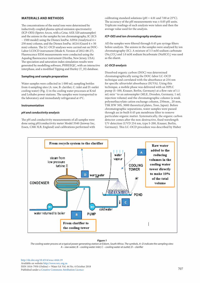
Water samples were collected in 1 000 mL sampling bottles from 4 sampling sites (A: raw, B: clari�er, C: inlet and D: outlet cooling water) (Fig. 1) in the cooling water processes at Kriel and Lethabo power stations. �e samples were transported to the laboratory and immediately refrigerated at 4°C.

Instrumentation

pH and conductivity analysis

�e pH and conductivity measurements of all samples were done using pH/conductivity meter Model 3540 (Jenway Inc, Essex, CM6 3LB, England) and calibrations performed with

calibrating standard solutions (pH = 4.01 and 7.00 at 25°C). �e accuracy of the pH measurements was ± 0.05 pH units. Triplicate readings of each analysis were taken and then the average value used for the analysis.

ICP-OES and ion chromatography analyses

All the samples were �ltered through 0.45 µm syringe �lters before analysis. �e anions in the samples were analysed by ion chromatography (IC). A mixture of 3.5 mM sodium carbonate (Na2CO3) and 1.0 mM sodium bicarbonate (NaHCO3) was used as the eluent.

LC-OCD analysis

Dissolved organic carbon (DOC) was determined chromatographically using the DOC-labor LC-OCD technique and correlated with the absorbance at 254 nm for speci�c ultraviolet absorbance (SUVA). Using this technique, a mobile phase was delivered with an HPLC pump (S−100, Knauer, Berlin, Germany) at a �ow rate of 1.1 mL·min−1 to an autosampler (MLE, Dresden, Germany, 1 mL injection volume) and the chromatographic column (a weak polymethacrylate cation exchange column, 250mm_ 20 mm, TSK HW 50S, 3000 theoretical plates, Toso, Japan). Before chromatographic separations, water samples were passed through an in-built 0.45 µm membrane �lter to remove particulate organic matter. Systematically, the organic carbon detector comes a�er the non-destructive, �xed wavelength UV-detection (UVD 254 nm, type S-200, Knauer, Berlin, Germany). �is LC-OCD procedure was described by Huber

Figure 1 The cooling water process at a typical power generating station at Eskom, South Africa. The symbols, A–D indicate the sampling sites:

A – raw water; B – cooling water inlet; C – cooling water at outlet; D – clari�er





Figure 2 FEEM spectral regions based on reported de�nite excitation (Ex) and emission (Em) wavelengths (adapted and redrawn from Gilmore et al., 2003)

et al. (2011). �e procedure includes acidi�cation of the water samples at the inlet of the OCD (at a �ow rate of 0.2 mL·min−1) to convert carbonates to carbonic acid. �is initial stripping process removes all inorganic carbon. Subsequent steps involving analysis of organic carbon were done by wet oxidation. �e oxygen required to oxidize DOC comes from water by a process called radiolysis of water at 185 nm. �is way, most compounds including �uoro-organic compounds, were oxidized. �e organic carbon detector (OCD) calibration was based on potassium hydrogen phthalate. In this case, the carbon mass was used to calibrate the OCD and its extinction coe�cient, ε = 1.683 × 10−3 L·mol−1·cm−1, used to calibrate the UVD (Huber et al., 2011).

Fluorescence excitation-emission matrices (FEEM)

Fluorescence emission excitation matrices (FEEMs) were collected using a Horiba AquaLog Spectrometer (Jvon, New Jersey, USA). No pre-treatment of the samples was applied. Maintaining a common pH between samples ensures that the �uorescence characteristics of the acidic functional groups in humic molecules remain constant. For this reason, all the samples were adjusted to a pH of 7. Collection of intensity values was at 10 nm increments within excitation-emission ranges of 250–450 nm and 300–600 nm, respectively. Scan rate was set to 600 nm·min−1, slit width was set to 10 nm and photomultiplier tube voltage was set to 775 V. Type 1 water at pH of 7 was used as a blank solution. �e �uorescence spectrometer used a xenon lamp excitation source and the emission at longer wavelengths was detected at 0.3 nm steps. Further to this, inner-�lter correction and Rayleigh scattering was applied to the data.

In this study, �uorescence was carried out under dilute sample conditions, which follows the equation:

(1)

where IO is the exciting light intensity, AbsOV is the number of quanta absorbed in the overlap region (OV) and ØF is the ratio of the quanta emitted to the quanta absorbed. �e spectra obtained were corrected for instrumental and sample dependent spectral anomalies such as the inner-�lter e�ects associated with sample absorbance of excitation and emission (Rayleigh scattering). Appropriately, spectral data can be compared to standard data and regions in literature and qualitative and quantitative NOM details will be drawn. Figure 2 shows some literature-based spectral regions using de�ned excitation and emission wavelength boundaries (Gilmore et al., 2003).

Peaks at shorter excitation wavelengths (280 nm) and longer emission wavelengths (> 380 nm) are associated with humic acid–like compounds. �is NOM-related spectral information lacks capabilities of quantifying multiple broad-shaped EEM peaks. Chen et al. (2003) postulated that integration beneath EEMs within selected regions would represent cumulative �uorescence responses of NOM with similar properties. �is technique shows that the volume Фi beneath a region said to be i of an EEM be calculated by Eq. 2:

𝐹𝐹 ∝ 𝐼𝐼� ∗ 𝐴𝐴𝐴𝐴𝐴𝐴�� ∗ ∅𝐹𝐹 (1)

Φ� = ∫ ∫ I(λ��λ��)dλ��dλ��

��

�� (2)

𝑋𝑋��=∑ 𝑎𝑎��𝐴𝐴��𝑐𝑐�� + 𝜀𝜀�� i = 1,…I; j = 1,…,k = 1,…K; (3)

log 𝛾𝛾 = 𝐴𝐴𝛾𝛾��

√I1 + 𝑎𝑎�

�𝐵𝐵�√I+ 𝐵𝐵𝐼𝐼

(4)

𝑃𝑃 = 𝐴𝐴� + 𝐴𝐴� ��

− ��

� + A�ln � ��

� + 𝐴𝐴��𝑇𝑇 − 𝑇𝑇�� + 𝐴𝐴��𝑇𝑇� − 𝑇𝑇�� + 𝐴𝐴� � �

�� − ��

�� (5)

𝐴𝐴� + 𝐵𝐵� = 𝐴𝐴𝐵𝐵 + 𝑔𝑔 + 𝑙𝑙 (6)

𝑆𝑆 = 𝐼𝐼𝐴𝐴𝑃𝑃𝐾𝐾�

= ⌈𝐴𝐴�⌉[𝐵𝐵�]

𝐾𝐾�

(7)

(2)

where dλem is the excitation wavelength interval (taken as 10 nm), dλem is the emission wavelength interval (taken as 0.5 nm), and I(λexλem) is the �uorescence intensity at each excitation-emission wavelength pair. �e values of Фi can be normalized to a DOC concentration of 1 mg·L−1 for comparison of EEMs from di�erent sources of NOM (Zhou et al., 2005).

Via ParaFac modelling, di�erences in the spectral slopes have been related to the proportional contribution of UV-B


Φ� = ∫ ∫ I(λ��λ��)dλ��dλ��

��

�� (2)



√I1 + 𝑎𝑎�


(4)

𝑃𝑃 = 𝐴𝐴� + 𝐴𝐴� ��

− ��

� + A�ln � ��

� + 𝐴𝐴��𝑇𝑇 − 𝑇𝑇�� + 𝐴𝐴��𝑇𝑇� − 𝑇𝑇�� + 𝐴𝐴� � �

�� − ��

�� (5)



= ⌈𝐴𝐴�⌉[𝐵𝐵�]

𝐾𝐾�

(7)





absorption coe�cients to the CDOM spectra which, as literature suggests, is dependent on the di�erent CDOM sources in natural waters (Guéguen et al., 2011). �is model factorizes a spectral matrix into three sub-matrices using the same number of factors in Eq. 3. �erefore, the F-EEM data is broken down into a set of tri-linear terms and a residual array.


Φ� = ∫ ∫ I(λ��λ��)dλ��dλ��

��

�� (2)



√I1 + 𝑎𝑎�


(4)

𝑃𝑃 = 𝐴𝐴� + 𝐴𝐴� ��

− ��

� + A�ln � ��

� + 𝐴𝐴��𝑇𝑇 − 𝑇𝑇�� + 𝐴𝐴��𝑇𝑇� − 𝑇𝑇�� + 𝐴𝐴� � �

�� − ��

�� (5)



= ⌈𝐴𝐴�⌉[𝐵𝐵�]

𝐾𝐾�

(7)

(3)

Equation 3 is the ParaFac equation in which Xijk is the �uorescence intensity of emission sample I at the j th emission wavelength and the kth excitation wavelength for ParaFac model with F number of components. �e terms a, b, and c represent the concentration, emission spectra, and excitation spectra, respectively, of the di�erent �uorophores. �e aif term is directly proportional to the concentration of the f th analyte of the ith sample, while b� and ckf are scaled estimates of the emission and excitation spectra at wavelengths j and k, respectively, for the f th analyte. �e εijk term represents any unexplained signal resulting from residual noise or un-modelled variability (Gentry-Shields et al., 2013). Evidence suggests that with the ParaFac model, four fluorescent components are identifiable: a protein-like component, soluble microbial by-product-like component, non-humic-like component and fulvic-like component (Guo et al., 2012).

Modelling using PHREEQC-Interactive

�e geochemical code, PHREEQC, was used to calculate the aqueous speciation and saturation indices of di�erent mineral phases. �e phases included aragonite, calcite, gypsum, magnesite, anhydrite and dolomite. During the assessment of the impact of humic substances on speciation and saturation indices, PHREEQCI databases were modi�ed before calculations. PHREEQC Version 3 implements many types of aqueous models, among them the following: ion-association aqueous models (the Lawrence Livermore National Laboratory model and WATEQ4F), a Pitzer speci�c-ion-interaction aqueous model, and the SIT (Speci�c ion Interaction �eory) aqueous model (Parkhurst and Appelo, 2013). Using these aqueous models, PHREEQC is able to carry out the following simulations: ion speciation (output including saturation indices), batch-reaction modelling (including equilibrium phases), surface complexation and ion exchange, reaction (addition/removal of speci�ed elements), mixing waters and changing temperature, transport modelling, advection with reactions with and without dispersion, and inverse modelling, and can calculate reactions that account for changes in composition of water along a �ow path (Parkhurst and Appelo, 2013).

Database modi�cation

�e speci�c database used in PHREEQC for the simulations is based on various approaches such as (i) the ion association approach (these include phreeqc.dat, wateq4f.dat, minteq.dat, llnl.dat, iso.dat and phreeqd.dat (Charlton and Parkhurst, 2011); (ii) the di�usion coe�cients: multicomponent di�usion, speci�c conductance; iii) molar volumes for calculation of density; and iv) the Pitzer speci�c interaction approach – Pitzer.dat. Various databases are based on the equations that de�ne activity coe�cients for model solutions and reactions and are discussed in this section. For example, the Lawrence Livermore National Laboratory aqueous model (LLNL) uses the following expression (Eq. 4) for the log (base 10) of an activity (Charlton and Parkhurst, 2011):


Φ� = ∫ ∫ I(λ��λ��)dλ��dλ��

��

�� (2)



√I1 + 𝑎𝑎�


(4)

𝑃𝑃 = 𝐴𝐴� + 𝐴𝐴� ��

− ��

� + A�ln � ��

� + 𝐴𝐴��𝑇𝑇 − 𝑇𝑇�� + 𝐴𝐴��𝑇𝑇� − 𝑇𝑇�� + 𝐴𝐴� � �

�� − ��

�� (5)



= ⌈𝐴𝐴�⌉[𝐵𝐵�]

𝐾𝐾�

(7)

(4)

where Aγ is the Debye-Hückel A parameter corresponding to –dh_a, Bγ is the Debye-Hückel B parameter corresponding to −dh_b, B is the Debye-Hückel B- dot parameter corresponding to -bdot, ai

0 is the hard-core diameter, which is speci�c to each aqueous species, and I is the ionic strength. �e LLNL_AQUEOUS_MODEL_PARAMETERS data block de�nes Aγ, Bγ and B as functions of temperature (Charlton and Parkhurst, 2011).

�e P�zer database is based on the P�zer activity coe�cients. Equation 5 shows the expression for a Pitzer parameter, P with T as the temperature in Kelvin, and Tr as the reference temperature (298.15 K). If less than 6 parameters are de�ned, the unde�ned parameters are assumed to be zero. When modifying a Pitzer aqueous interaction parameter, care is needed to ensure thermodynamic consistency among all the parameters. If the same type of parameter with the same set of species is rede�ned, even if the order of the species is di�erent, then the previous de�nition is removed and replaced with the new de�nition (Charlton and Parkhurst, 2011).


Φ� = ∫ ∫ I(λ��λ��)dλ��dλ��

��

�� (2)



√I1 + 𝑎𝑎�


(4)

𝑃𝑃 = 𝐴𝐴� + 𝐴𝐴� ��

− ��

� + A�ln � ��

� + 𝐴𝐴��𝑇𝑇 − 𝑇𝑇�� + 𝐴𝐴��𝑇𝑇� − 𝑇𝑇�� + 𝐴𝐴� � �

�� − ��

�� (5)



= ⌈𝐴𝐴�⌉[𝐵𝐵�]

𝐾𝐾�

(7)

(5)

Carefully, therefore, the humate and fulvate thermodynamic de�nitions were incorporated into a Tipping and Hurley database with a WHAM (T_H.DAT) (Tipping, 2002), which de�nes the LLNL and the P�zer databases. Table 1 shows the log k values for equilibrium phase equations of the reactions incorporated into the T_H.DAT database together with their stability constants, all drawn from visual MINTEQ v 3.1.1. For these reactions, the phases were de�ned as SOLUTION_SPECIES in T_H.DAT.

�e simulation mixture comprised of scale-forming cations (Ca2+ and Mg2+) and anions (SO4

2- , Cl-, NO3-) de�ned

as SOLUTION_SPECIES. �e carbonate concentration was considered as alkalinity measured asHCO3

- which was also de�ned in SOLUTION_SPECIES block. Fulvate-2 and Humate-2, have been previously de�ned as SOLUTION_MASTER_SPECIES in the Tipping and Hurley WHAM model (2003). �e modi�ed T_H.DAT incorporates log k values from risbergfa13.vdb, shmgeneric10.vdb, genericha08.nic and genericfa08.nic databases in visual MINTEQ version 3.1. �ese values de�ne the equilibrium phase equations of NOM (humic and fulvic acid) with Mg2+ and Ca2+ that give rise to CaFulvate, MgFulvate, CaHumate and MgHumate (Fig. 3).

TABLE 1Equilibrium phase equations de�ned in T_H.DAT as

SOLUTION_SPECIES using the NICA-Donnan visual MINTEQ

Phase Equilibrium reaction Log k

#CaFulvate Ca+2 + Fulvate-2 = CaFulvate −3#MgFulvate Mg+2 + Fulvate-2 = MgFulvate –2.4#CaHumate Ca+2 + Humate-2 = CaHumate 0.43#MgHumate Mg+2 + Humate-2 = MgHumate 0.60


Φ� = ∫ ∫ I(λ��λ��)dλ��dλ��

��

�� (2)



√I1 + 𝑎𝑎�


(4)

𝑃𝑃 = 𝐴𝐴� + 𝐴𝐴� ��

− ��

� + A�ln � ��

� + 𝐴𝐴��𝑇𝑇 − 𝑇𝑇�� + 𝐴𝐴��𝑇𝑇� − 𝑇𝑇�� + 𝐴𝐴� � �

�� − ��

�� (5)



= ⌈𝐴𝐴�⌉[𝐵𝐵�]

𝐾𝐾�

(7)





Mineral saturation

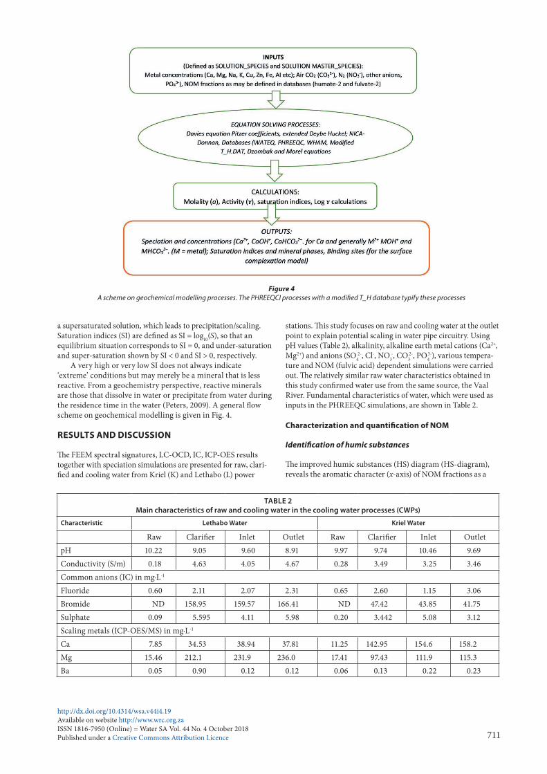
�e pH, alkalinity, metal cations and anions were modelled together with organic components (fulvates) using a fulvate-adjusted T_H database. �e input-output geochemical execution processes on the PHREEQC code are summarised in Fig. 4. To show mineral dissolution or precipitation, saturation indices (SI) were calculated. Herein, a general reaction (Eq. 6), describes super-saturation which is the key parameter that determines precipitation. �e saturation ratio (S) is described as the ratio of the ionic activity product (IAP) to the equilibrium constant (Ks) (Eq. 7).

(6)

where A- is the anion being equilibrated (A- = (SO42- , Cl-, NO3

-, CO3

2-, PO43-), B+ is the metal cation, AB is the mineral phase

formed and g and l are any gas or liquid phases, respectively.


Φ� = ∫ ∫ I(λ��λ��)dλ��dλ��

��

�� (2)



√I1 + 𝑎𝑎�


(4)

𝑃𝑃 = 𝐴𝐴� + 𝐴𝐴� ��

− ��

� + A�ln � ��

� + 𝐴𝐴��𝑇𝑇 − 𝑇𝑇�� + 𝐴𝐴��𝑇𝑇� − 𝑇𝑇�� + 𝐴𝐴� � �

�� − ��

�� (5)



= ⌈𝐴𝐴�⌉[𝐵𝐵�]

𝐾𝐾�

(7)

(7)

A value of S < 1, indicates an under-saturated solution, S = 1 shows a solution in equilibrium with the solid, while S > 1 shows


Φ� = ∫ ∫ I(λ��λ��)dλ��dλ��

��

�� (2)



√I1 + 𝑎𝑎�


(4)

𝑃𝑃 = 𝐴𝐴� + 𝐴𝐴� ��

− ��

� + A�ln � ��

� + 𝐴𝐴��𝑇𝑇 − 𝑇𝑇�� + 𝐴𝐴��𝑇𝑇� − 𝑇𝑇�� + 𝐴𝐴� � �

�� − ��

�� (5)



= ⌈𝐴𝐴�⌉[𝐵𝐵�]

𝐾𝐾�

(7)

Figure 3Modi�cation of the Tipping and Hurley database with WHAM (T_H.DAT) to include humates and fulvates. The speciation outputs of equilibrium

reaction de�nitions in Table 1 are shown under modi�ed T-H.DAT.





a supersaturated solution, which leads to precipitation/scaling. Saturation indices (SI) are de�ned as SI = log10(S), so that an equilibrium situation corresponds to SI = 0, and under-saturation and super-saturation shown by SI < 0 and SI > 0, respectively.

A very high or very low SI does not always indicate ‘extreme’ conditions but may merely be a mineral that is less reactive. From a geochemistry perspective, reactive minerals are those that dissolve in water or precipitate from water during the residence time in the water (Peters, 2009). A general �ow scheme on geochemical modelling is given in Fig. 4.

RESULTS AND DISCUSSION

�e FEEM spectral signatures, LC-OCD, IC, ICP-OES results together with speciation simulations are presented for raw, clari-�ed and cooling water from Kriel (K) and Lethabo (L) power

stations. �is study focuses on raw and cooling water at the outlet point to explain potential scaling in water pipe circuitry. Using pH values (Table 2), alkalinity, alkaline earth metal cations (Ca2+, Mg2+) and anions (SO4

2-, Cl-, NO3-, CO3

2-, PO43-), various tempera-

ture and NOM (fulvic acid) dependent simulations were carried out. �e relatively similar raw water characteristics obtained in this study con�rmed water use from the same source, the Vaal River. Fundamental characteristics of water, which were used as inputs in the PHREEQC simulations, are shown in Table 2.

Characterization and quanti�cation of NOM

Identi�cation of humic substances

�e improved humic substances (HS) diagram (HS-diagram), reveals the aromatic character (x-axis) of NOM fractions as a

Figure 4A scheme on geochemical modelling processes. The PHREEQCI processes with a modi�ed T_H database typify these processes

TABLE 2Main characteristics of raw and cooling water in the cooling water processes (CWPs)

Characteristic Lethabo Water Kriel Water

Raw Clari�er Inlet Outlet Raw Clari�er Inlet OutletpH 10.22 9.05 9.60 8.91 9.97 9.74 10.46 9.69Conductivity (S/m) 0.18 4.63 4.05 4.67 0.28 3.49 3.25 3.46Common anions (IC) in mg·L-1

Fluoride 0.60 2.11 2.07 2.31 0.65 2.60 1.15 3.06Bromide ND 158.95 159.57 166.41 ND 47.42 43.85 41.75Sulphate 0.09 5.595 4.11 5.98 0.20 3.442 5.08 3.12Scaling metals (ICP-OES/MS) in mg·L-1

Ca 7.85 34.53 38.94 37.81 11.25 142.95 154.6 158.2Mg 15.46 212.1 231.9 236.0 17.41 97.43 111.9 115.3Ba 0.05 0.90 0.12 0.12 0.06 0.13 0.22 0.23





function of their molecularity (y-axis) (Fig. 5a). �is diagram is a plot of the spectral absorption coe�cient (SAC) to the organic carbon (OC) ratio (aromaticity) of a HS-fraction against its nominal molecular weight (Mn) (Huber et al., 2011). Accordingly, the curved boundaries de�ne the region where the humic substances are characterized. �e humic substances area was developed using fulvic and humic acid characteristics of water samples from di�erent sources discussed in Huber et al. (2011). As reported in Huber et al. (2011), the humic acid (HA) and fulvic acid (FA) standard (II) isolates of the International Humic Substances Society (IHSS) were used to calibrate the HS molecular weights, prior to all characterizations. In the current study, raw and cooling water samples from Kriel and Lethabo power stations, were characterized. �e results obtained showed that raw, clari�er and cooling water (inlet and outlet) from Kriel (shown by K) and Lethabo (shown by L) consists mainly of pedogenic fulvic acids (Fig. 5a). �e fulvic acid character increased in the order of E > A > G, B and C > H and F > D. �e raw water data points A and E, from Kriel and Lethabo, respectively, are close to each other in the HS-diagram (Fig. 5a). �is con�rms the common source of cooling water used at these Eskom power stations, i.e., the Vaal river. �e FA reported in this study is in close agreement with data reported by Huber et al. (2011), regarding the characteristics on the HS-diagram FA obtained from the river Rhine, river Seine and Steinbach surface water (Huber et al., 2011). However, the FA obtained from our study di�ers from the FA reported by Huber et al. (2011) on data obtained for river Westend, Lake Sosa, Lake Galilee and Caspian Sea waters. �is variation in results further reveals the di�erence in surface origin of the FA obtained in our study, which was predominant in the cooling water analysed in this study.

Quanti�cation of NOM fractions

Natural surface waters exhibit 5 distinct peaks corresponding to LC-OCD elutes of di�erent NOM fractions, namely: (i)

Figure 5aThe HS-diagram for humic fractions in cooling water samples from the Kriel (K) and Lethabo (L) power stations. Aromaticity of aquatic humic

substances is measured as the SAC/OC ratio, which is plotted against molecularity (Mn values (nominal molecular weights)). (A: K-Raw; B: K-outlet CW; C: K-inlet CW; D: K-clari�er; E: L-Raw; F: L-clari�er; G; L-inlet CW; H: L-outlet CW). The calibration water sources are adapted from by Huber et al., 2011.

Figure 5bChromatograms of water in the CWP (Kriel and Lethabo power

generating companies, South Africa), based on Fig. 5a with �tted peaks for HS and �tted boundaries for non-humic matter.





biopolymers; (ii) humic substances; (iii) building blocks; (iv) low molecular weight acids and (v) low molecular weight neutrals. �e major components of the humic substances’ fraction, the HA and FA elute at 43.4 and 46.7 min, respectively (Huber et al., 2011). Fig. 3b shows chromatograms corresponding to the NOM fractions analysed by LC-OCD.

Table 3 summarizes the LC-OCD quantitative results, based on the raw and cooling water samples from the two power stations. �ese results include the humic substances which were predominantly fulvic acid, shown in Fig. 5b. For all samples, the humic substances fraction quantities did not di�er signi�cantly with total dissolved organic carbon (DOC) (r2 = 0.01677, p < 0.05, ANOVA). For example, the percentage HS concentration to the total DOC in the raw water was 88.4% and 89.5% for samples from Kriel and Lethabo power stations, respectively. Separately, a similar observation was made using cooling water, i.e., 87.8% and 83.5% for Kriel and Lethabo, respectively. However, the raw and cooling water HS fractions from the power stations di�ered signi�cantly (r2 = 0.95, p < 5, ANOVA).

Table 3 also shows the SUVA values corresponding to the various samples. NOM is hydrophilic (HPI) if the speci�c UV absorbance at λ254 (SUVA) value < 2 (an indication of non humic substances), hydrophobic (HPO) with a SUVA value > 4 (an indication of humic substances) and is transphilic (TPI, a mixture of both HPO and HPI) if 2 ≤ SUVA ≤ 4. In the present study, the SUVA values of the water samples generally show that the nature of humic substances is highly aromatic. �is is supported by the high percentage of HS in dissolved organic carbon (DOC). Similar studies have shown that surface water from di�erent sources contains a NOM matrix comprising of transphilic, hydrophobic and hydrophilic compounds (Filloux et al., 2012, Zhou et al., 2014). �e percentage of humic substances reported by Zhou et al. (2014) (84%) agree with the LC-OCD results obtained in this study for the raw and cooling water processes (ranging from 80–90%).

FEEM characterization of NOM

Typical FEEM spectra of cooling water used at the Kriel power station are presented in Fig. 6. Generally, the observed excitation (EX) and emission (EM) spectra for water samples con�rmed intense fulvic acid and humic acid activities. �ese

TABLE 3Structural qualities of DOC and quantity of HS obtained with LC-OCD for Kriel (K) and Lethabo (L)

power stations (*% HS is calculated as (HS/DOC) × 100; *BBs represents building blocks)

Sample DOC (mg·L-1) HS (mg·L-1) %* HS BBs as % of HS SUVA SAC/DOC (L·mg-1·m-1)

K-Raw 5.934 5.244 88.4 12.548 5.18K-CWO 49.290 43.282 87.8 13.534 4.36K-CWI 47.023 40.574 86.3 15.769 4.40K-Clari�er 81.422 68.849 84.6 14.715 3.40L-Raw 4.022 3.599 89.5 10.475 6.58L-Clari�er 45.902 36.741 80.0 23.162 3.36L-CWI 25.830 21.714 84.1 18.698 4.97L-CWO 38.775 32.378 83.5 18.374 3.93

Figure 6 Typical �uorescence excitation-emission matrices of raw water (a), clari�ed water (b) and cooling water (c). The x-axis shows the range

of excitation (EX) wavelength (220–350 nm) and the y-axis shows the emission (EM) wavelength range (220–610 nm)





observations complement the LC-OCD results presented in Table 3. �e spectral signatures, as revealed by FEEM (Fig. 6), showed intense activity of HS at λEX 250–290/λEM 350–500 nm, which further con�rmed the predominance of fulvic acid in the NOM. �e fulvic acid FEEM spectral regions have been reported elsewhere (Ahmed et al., 2014).

�e observed raw and cooling water characteristics of NOM using LC-OCD and FEEM (found to be predominantly FA), and the quantitative measurements of HS (established to be FA), formed the basis of modelling discussions under the geochemical sub-heading. �ese include database modi�cations and the use of the PHREEQC code to include FA equilibrium reactions with selected cations.

Geochemical modelling

At ambient temperature (25°C), the selected minerals (aragonite, dolomite, gypsum, calcite and magnesite) showed higher dissolution than precipitation (Fig. 7). �ese results were further simulated in an extended range of temperatures and the concentration of fulvic acid. Mineral phase modeling, using F_H.DAT, showed distinct saturation patterns. Saturation indices of selected phases are discussed in this article, including: the two polymorphs of calcium carbonate, namely; aragonite (CaCO3) and calcite (CaCO3), anhydrite (CaSO4), gypsum (CaSO4·2H2O), dolomite CaMg(CO3)2 and magnesite (MgCO3). Both alkalinity de�ned as HCO3

- and sulphur-compounds in the form of SO4

2- values were calculated as averages of raw and cooling water from Lethabo power station. From Fig. 7, the saturation levels revealed variations depending on the source of water. �is conforms to what is expected as the cooling water evaporates. As the water gets recycled over and over, its components concentrate. �e in�uence of temperature and concentration of humic substances on formation and saturation of these mineral phases are modelled in this section.

Temperature-dependence mineral simulations

Temperature simulations revealed 2 types of mineral phase occurrences: (i) mineral phases below and above the saturation lines (Fig. 8) showing under-saturation and supersaturation (calcite, aragonite, dolomite and magnesite), respectively; (ii) mineral phases showing under-saturation only (anhydrite and

Figure 7Saturation index levels of selected mineral assemblages using a modi�ed F_H.DAT on the PHREEQCI code. Anhydrite, aragonite, calcite, dolomite,

gypsum and magnesite represent selected mineral phases.

Figure 8 Predictive saturation indices of mineral assemblages based on temperature, viz, calcite, aragonite, dolomite, anhydrite, gypsum and magnesite

(K and L represent water drawn from Kriel and Lethabo, respectively)





gypsum). �e saturation indices of minerals were calculated from the F_H.DAT. Calcite (CaCO3) was found to have higher saturation indices than aragonite (CaCO3). For example, in almost all (except raw water samples) calcite showed supersaturation at lower temperatures than aragonite. A very speci�c illustration is the precipitation of calcite and aragonite in the Kriel clari�er (K-clari�er) and Kriel cooling water outlet (K-CWO), from 15°C and 30°C, respectively (Fig. 8 Calcite, and Fig. 8 Aragonite). It is important to mention that crystals of CaCO3 exist in di�erent polymorphs, i.e., calcite, aragonite and vaterite. Calcite is the most stable of the three while vaterite is the least stable. Ideally, they form under di�erent conditions, for the same amounts of inputs (Wada et al., 2013). Aragonite is a high-pressure phase which changes to calcite at ambient conditions. Its precipitation is dependent on pH, temperature, super-saturation and CO2 content.

�e relatively high degree of under-saturation of gypsum (CaSO4·2H2O) and anhydrite form (CaSO4) compared to other mineral phases is likely to be due to the low concentration of sulphate ions in the cooling and raw water samples (Fig. 8 gypsum; Fig. 8 anhydrite). Gypsum and anhydrite dissolution were apparent in most of the water samples, thus contributing free Ca2+ that enhances calcite precipitation, a phenomenon called common ion driven precipitation (CIDP). We noted that calcium concentrations are controlled by calcite and aragonite dissolution. Furthermore, the dynamics of Ca complexation and dissolution govern its pH-dependent equilibria (Pokrovsky et al., 2009). Pokrovsky et al. (2009) provided a detailed argument on the dissolution kinetics and precipitation of dolomite and magnesite, in addition to calcite, as a function of pH, temperature and pressure. �ey noted that the rate constants of dissolution of these minerals increase with increase in pH and temperature. �is agrees with the temperature-dependent simulation results in this study.

Speciation simulations based on NOM (fulvic acid)

�e concentrations of fulvic acid were determined to be in the range 3.5 to 81.5 mg·L−1 ,viz, (i)) Lethabo had concentrations as follows: raw 4.022 mg·L−1, clari�er 45.902 mg·L−1, CWI 25.830 mg·L−1 and CWO 38.775 mg·L−1, compared to (ii) Kriel’s raw 5.934 mg·L−1, clari�er 81.422 mg·L−1, CWI 47.023 mg·L−1 and

CWO 49.290 mg·L−1 (Table 3). Raw water fulvics were compared with those from the clari�er as well as those from the cooling water tower. As expected, the results showed that the fulvics from the cooling tower were found to be less than a tenth of those from the clari�er. �is may be attributed to the fact that recycled water volumes keep decreasing due to the evaporative processes in the cooling water chambers and this concentrates the humic substances (Pather, 2004). Various exponents of the experimental fulvic acid concentrations were inputted to the PHREEQC SOLUTION_SPECIES using the F_H.DAT and the results are presented in Figs 9 and 10.

How available and reliable are the thermodynamic and equilibrium de�nitions of NOM in the existing databases? Undoubtedly, no single modi�cation would suit all organic compounds. Huber et al. (2012) agree with this. In their simulations, they chose to pick thermodynamic de�nitions of volatile fatty acids (acetate, propionate, butyrate and lactate) from MINTEQ.V4.DAT and included them in the PHREEQC code with interactive interface (PHREEQCI) database (Huber et al., 2012). �erefore, to answer the question, the F_H.DAT was constructed using available thermodynamic de�nitions for the Ca and Mg-fulvate equilibrium phases in Visual MINTEQ.v3.1.1. �is work drew up speci�c species-oriented modi�cations on the premise that variability of both the physico-chemical conditions and the wide range of compounds in cooling water play a critical role in data generation.

Based on the expanded fulvic acid simulations from our study, the e�ect of fulvate ions as de�ned in the EQUILIBRIUM_PHASE and SOLUTION_MASTER_SPECIES in the F_H.DAT was investigated. Results show that by changing the fulvic acid concentrations in cooling water processes, one can alter scaling indices of mineral phases signi�cantly (Figs 9 and 10). �ese �gures are extracts of the raw and cooling water results at Kriel power station. �is reduction may be attributed to the formation of the de�ned complexes between Ca/Mg and fulvic acid, viz, MgFulvate and CaFulvate.

Scale control modelling studies

In this article, the composition of scale in pipes, with physico-chemical conditions determined, is given in Table 4. �e experimental results shown in Table 4 were obtained from

Figure 9 Extrapolated mineral phase curves based on raw water concentrations

at Kriel. Various exponents of the experimental fulvic acid concentrations were input parameters into the PHREEQC SOLUTION_

SPECIES using the F_H.DAT.

Figure 10Extrapolated mineral phase curves on a reduced scale on x-axis showing

the concentration of fulvic acid (0–6 000 mg·L-1)





analysis of a scale sample obtained from cooling water pipes at Lethabo. Accordingly, the results showed varied concentrations of elements in the order of Zn > Al > Ca > Mg for the 4 metal ions under consideration.

�e second step was to accurately determine the content of scaling metals and other trace elements in water. �e fundamental objective in the current context is to keep Ca/Mg ions in solution (complexed form). �erefore, it was important to include organic compounds in the PHREEQC databases and simulate scale formation under di�erent conditions (shown in the methodology section). In that section, a typical illustration

of precipitative and complexation processes has been discussed using the context of fulvic acid interactions with metal cations.

Table 5 shows potential scaling potentials of selected mineral phases of Ca and Mg in water; aragonite (CaCO3), artinite (MgCO3:Mg(OH)2:3H2O), brucite (Mg(OH)2), calcite (CaCO3), dolomite (CaMg(CO3)2), dolomite(d) CaMg(CO3)2, huntite (CaMg3(CO3)4), hydromagnesite (Mg5(CO3)4(OH)2:4H2O) and magnesite (MgCO3). From this study, the interaction between calcium and carbonate ions is de�ned to in�uence scaling in water pipes. �e saturation indices of aragonite and calcite (polymorphs of CaCO3) are positive throughout the recycle water processes (in raw and in cooling water). From the study, these polymorphs remained relatively stable throughout the recycle processes.

�e third step is to consider the current state Ca binding to fulvic acid, in raw water compared to recycled cooling water. For instance, the molality values of CaFulvate are lower (viz; 4.6 × 10−13 and 1.5 × 10−11) in raw water at Lethabo and Kriel, respectively. �is complex is 100-fold higher in cooling water than in raw water (Table 6). A similar scenario is experienced with MgFulvate. �is phenomenon explains the fact that cooling recycled volumes have reduced precipitation potentials for Mg and Ca. �is leads to the conclusion that manipulation of physicochemical parameters enhances complexation of Ca and Mg, which inhibits complexation of non-scaling metals while reducing the components that oxidise, which is critical in scale control.

TABLE 4Selected sample XRF results of the components of scale

obtained from Lethabo cooling water pipes

Mineral phase Formula % by mass Total

Zn mineral phasesSmithsonite Zn(CO3) 0.4 48.5Zinc phosphate Zn(PO3)2 28.3Zinkosite, syn ZnSO4 19.8Al mineral phasesBerlinite; berlinite, syn

Al(PO4) 35.6 36.9

Diaspore, syn AlO(OH) 1.3Ca mineral phasesCalcium iron(II) oxide

CaFeO2 5.5 14.1

Gypsum CaSO4·2H2 O 0.6Calcium silicide CaSi2 0.3Aragonite Ca (CO3) 7.5Dolomite Ca Mg (CO3)2 0.2Mg mineral phasesMagnesite, syn Mg (CO3) 0.5 0.7Dolomite Ca Mg (CO3)2 0.2

TABLE 5Saturation indices of various mineral phases of Ca and Mg

Lethabo station Kriel station

Saturation indices

Mineral phase Raw water Cooling water Raw water Cooling water

Anhydrite (CaSO4) −5.8 −3.6 −5.3 −3.2Aragonite (CaCO3) 0.9 0.7 1.0 1.8Artinite (MgCO3:Mg(OH)2:3H2O) 0.6 −0.6 0.1 0.8Brucite (Mg(OH)2) 0.2 −1.3 -0.2 −0.1Calcite (CaCO3) 1.1 0.9 1.1 2.0Dolomite (CaMg(CO3)2) 2.8 2.9 2.8 4.2Dolomite(d) CaMg(CO3)2 2.3 2.4 2.3 3.6Epsomite (MgSO4:7H2O) −7.5 −4.8 −7.0 −5.4Gypsum (CaSO4:2H2O) −5.6 −3.4 −5.0 −3.0Huntite (CaMg3(CO3)4) 2.0 2.6 1.9 4.3Magnesite (MgCO3) 1.2 1.5 1.1 1.6Nesquehonite (MgCO3:3H2O) −1.2 −0.9 −1.3 −0.8Portlandite (Ca(OH)2) −6.3 −8.3 −6.6 −6.1

TABLE 6Summary of the Ca/Mg fulvate complexes (in mols) in raw

and cooling water

Lethabo station Kriel station

Complexed species

Raw water Cooling water

Raw water Cooling water

Fulvate-2 5.5 × 10-6 5.0 × 10-5 8.1 × 10-6 1.1 × 10-4

HFulvate- 5.3 × 10-11 7.4 × 10-10 1.5 × 10-11 2.8 × 10-10

CaFulvate 4.6 × 10-13 1.4 × 10-11 1.1 × 10-12 1.3 × 10-10

MgFulvate 6.7 × 10-12 6.1 × 10-10 1.2 × 10-11 6.8 × 10-10





Given the results in Tables 5 and 6, we can conclude that complexation between Ca/Mg cations and fulvates could be linked to saturation indices in explaining the scaling potential. Saturation index results show that only the values in raw water samples are slightly di�erent. However, the fact is that the incorporation of the equilibrium equations for Ca and Mg with fulvates into the PHREEQC databases, could o�er a special link that explains simultaneous complexation and precipitation reactions in fresh waters used for industrial purposes. Modelling the formation of these discrete chemical complexes showed a reduction in the concentration of free Ca and Mg ions in solution, hence decreased scaling potential. In addition, the study has shown that the concentrations of fulvic acid and temperatures may be manipulated, and using the geochemical code PHREEQC, the incidence of scaling could be predicted and controlled.

CONCLUSIONS

�e HS-diagram revealed the predominance of the fulvic acid fraction of NOM in raw and cooling water. For all samples, the fulvic acid fraction did not di�er signi�cantly relative to total dissolved organic carbon. In addition, the spectral EEM signatures, showed intense activity of HS at λEX 250–290/λEM 350–500 nm, which con�rmed the predominance of fulvic acid in NOM. Using the PHREEQC code, the Tipping and Hurley database (T_H.DAT) was successfully modi�ed by including Mg and Ca complexation equilibrium equations with the fulvate ion. �is was achieved by incorporating Fulvate-2 complexation equilibria in the SOLUTION_MASTER_SPECIES block and de�ning it as SOLUTION_SPECIES. Both the humates and fulvates were incorporated in the T_H.DAT database correctly and were able to generate outputs on the PHREEQC code. As a result, new complexation the Ca-fulvate and Mg-fulvate mineral phase outputs were obtained and related to the scaling potential of Ca/Mg. Overall, the entire study has shown that if the concentrations of organics (such as fulvic acid) are known, the conditions that favour their complexation with Ca/Mg could be manipulated appropriately to control the incidence of scaling in pipe circuitry.

ACKNOWLEDGEMENTS

�e authors of this paper are grateful to the Centre for Nanomaterials Science Research and the Faculty of Science which hosts the Department of Applied Chemistry at the University of Johannesburg. Many thanks to David Parkhurst of the USGS for providing the authors with valuable information on the PHREEQC code.

REFERENCES

AHMED AM, HAMILTON-TAYLOR J, BIEROZA M, ZHANG H and DAVISON W (2014) Improving and testing geochemical speciation predictions of metal ions in natural waters. Water Res. 67 276–291. https://doi.org/10.1016/j.watres.2014.09.004

BRUNNER G (2014) Chapter 3 – Properties of mixtures with water. In: Gerd B (ed.) Supercritical Fluid Science and Technology. Elsevier, Amsterdam.

CHARLTON S and PARKHURST D (2011) Modules based on the geochemical model PHREEQC for use in scripting and programming languages. Comput. Geosci. 37 1653–1663. https://doi.org/10.1016/j.cageo.2011.02.005

CHRISTENSEN J, TIPPING E, KINNIBURGH D, GRØN C and CHRISTENSEN TH (1998) Proton binding by groundwater fulvic acids of di�erent age, origins, and structure modeled with the model V and NICA-Donnan model. Environ. Sci. Technol. 32 3346–3355. https://doi.org/10.1021/es971134o

FILLOUX E, GALLARD H and CROUE J (2012) Identi�cation of e�uent organic matter fractions responsible for low-pressure membrane fouling. Water Res. 46 5531–5540. https://doi.org/10.1016/j.watres.2012.07.034

GENTRY-SHIELDS J, WANG A, CORY RM and STEWART JR (2013) Determination of speci�c types and relative levels of QPCR inhibitors in environmental water samples using excitation–emission matrix spectroscopy and PARAFAC. Water Res. 47 3467–3476. https://doi.org/10.1016/j.watres.2013.03.049

GILMORE A, LARKUM A, SALIH A, ITOH S, SHIBATA Y, BENA C and VAN WOESIK R (2003) Simultaneous time resolution of the emission spectra of �uorescent proteins and zooxanthellar chlorophyll in reef building corals. Photochem. Photobiol. 77 515–523. https://doi.org/10.1562/0031-8655(2003)077<0515:STROTE>2.0.CO;2

GUÉGUEN C, GRANSKOG MA, MCCULLOUGH G and BARBER DG (2011) Characterisation of colored dissolved organic matter in Hudson Bay and Hudson Strait using parallel factor analysis. J. Mar. Syst. 88 423–433. https://doi.org/10.1016/j.jmarsys.2010.12.001

GUO X, HE X, ZHANG H, DENG Y, CHEN L and JIANG J (2012) Characterization of dissolved organic matter extracted from fermentation e�uent of swine manure slurry using spectroscopic techniques and parallel factor analysis (PARAFAC). Microchem. J. 102 115–122. https://doi.org/10.1016/j.microc.2011.12.006

GUSTAFSSON JP (2001) Modeling the acid–base properties and metal complexation of humic substances with the Stockholm Humic Model. J. Coll. Interf. Sci. 244 102–112. https://doi.org/10.1006/jcis.2001.7871

GUSTAFSSON JP and BERGGREN KD (2005) Modeling salt-dependent proton binding by organic soils with the NICA-Donnan and Stockholm Humic models. Environ. Sci. Technol. 39 5372–5377. https://doi.org/10.1021/es0503332

HOCH A, REDDY M and AIKEN G (2000) Calcite crystal growth inhibition by humic substances with emphasis on hydrophobic acids from the Florida Everglades. Geochim. Cosmochim. Acta 64 61–72. https://doi.org/10.1016/S0016-7037(99)00179-9

HUBER P, NIVELON S, OTTENIO P and NORTIER P (2012) Coupling a chemical reaction engine with a mass �ow balance process simulation for scaling management in papermaking process waters. Ind. Eng. Chem. Res. 52 421–429. https://doi.org/10.1021/ie300984y

HUBER SA, BALZ A, ABERT M and PRONK W (2011) Characterisation of aquatic humic and non-humic matter with size-exclusion chromatography–organic carbon detection–organic nitrogen detection (LC-OCD-OND). Water Res. 45 879–885. https://doi.org/10.1016/j.watres.2010.09.023

KOOPAL LK, SAITO T, PINHEIRO JP and VAN RIEMSDIJK WH (2005) Ion binding to natural organic matter: General considerations and the NICA–Donnan model. Coll. Surf. A: Physicochem. Eng. Aspects 265 40–54. https://doi.org/10.1016/j.colsurfa.2004.11.050

MILNE C, KINNIBURGH D, VAN RIEMSDIJK W and TIPPING E (2003) Generic NICA-Donnan model parameters for metal-ion binding by humic substances. Environ. Sci. Technol. 37 958–971. https://doi.org/10.1021/es0258879

PARKHURST D and APPELO C (2013) Description of input and examples for PHREEQC version 3: a computer program for speciation, batch-reaction, one-dimensional transport, and inverse geochemical calculations. US Geological Survey, Reston, Virginia.

PATHER V (2004) Eskom and water. Proc. 2004 Water Institute of Southern Africa (WISA) Biennial Conference, 26 May 2004, Cape Town, South Africa. URL: http://www.ewisa.co.za/literature/�les/260.pdf (Accessed October 2014).

PETERS C (2009) Accessibilities of reactive minerals in consolidated sedimentary rock: An imaging study of three sandstones. Chem. Geol. 265 198–208. https://doi.org/10.1016/j.chemgeo.2008.11.014

POKROVSKY O, GOLUBEV S, SCHOTT J and CASTILLO A (2009) Calcite, dolomite and magnesite dissolution kinetics in aqueous solutions at acid to circumneutral pH, 25 to 150° C and 1 to 55 atm: New constraints on CO2 sequestration in sedimentary basins. Chem. Geol. 265 20–32. https://doi.org/10.1016/j.chemgeo.2009.01.013

POURRET O, DAVRANCHE M, GRUAU G and DIA A (2007)




https://doi.org/10.1016/j.watres.2014.09.004

https://doi.org/10.1016/j.cageo.2011.02.005

https://doi.org/10.1016/j.cageo.2011.02.005

https://doi.org/10.1021/es971134o




https://doi.org/10.1562/0031-8655(2003)077%3c0515:STROTE%3e2.0.CO;2

https://doi.org/10.1562/0031-8655(2003)077%3c0515:STROTE%3e2.0.CO;2

https://doi.org/10.1016/j.jmarsys.2010.12.001

https://doi.org/10.1016/j.microc.2011.12.006

https://doi.org/10.1006/jcis.2001.7871

https://doi.org/10.1006/jcis.2001.7871

https://doi.org/10.1021/es0503332

https://doi.org/10.1016/S0016-7037(99)00179-9

https://doi.org/10.1021/ie300984y

https://doi.org/10.1021/ie300984y


https://doi.org/10.1016/j.colsurfa.2004.11.050

https://doi.org/10.1016/j.colsurfa.2004.11.050

https://doi.org/10.1021/es0258879

http://www.ewisa.co.za/literature/files/260.pdf

http://www.ewisa.co.za/literature/files/260.pdf

https://doi.org/10.1016/j.chemgeo.2008.11.014




Organic complexation of rare earth elements in natural waters: evaluating model calculations from ultra�ltration data. Geochim. Cosmochim. Acta 71 2718–2735. https://doi.org/10.1016/j.gca.2007.04.001

ROSENBERG YO, REZNIK I J, ZMORA-NAHUM S and GANOR J (2012) �e e�ect of pH on the formation of a gypsum scale in the presence of a phosphonate antiscalant. Desalination 284 207–220. https://doi.org/10.1016/j.desal.2011.08.061

TIPPING E (2002) Cation Binding by Humic Substances. Cambridge University Press, Cambridge, England. https://doi.org/10.1017/CBO9780511535598

WADA N, HORIUCHI N, NAKAMURA M, HIYAMA T, NAGAI A and YAMASHITA K (2013) E�ect of poly (acrylic acid) and

polarization on the controlled crystallization of calcium carbonate on single-phase calcite substrates. Crystal Growth Design 13 2928–2937. https://doi.org/10.1021/cg400337m

ZHANG F, YAN C, TENG HH, RODEN EE and XU H (2013) In situ AFM observations of Ca–Mg carbonate crystallization catalyzed by dissolved sul�de: Implications for sedimentary dolomite formation. Geochim. Cosmochim. Acta 105 44–55. https://doi.org/10.1016/j.gca.2012.11.010

ZHOU S, SHAO Y, GAO N, LI L, DENG J, TAN C and ZHU M (2014) In�uence of hydrophobic/hydrophilic fractions of extracellular organic matters of Microcystis aeruginosa on ultra�ltration membrane fouling. Sci. Total Environ. 471 201–207. https://doi.org/10.1016/j.scitotenv.2013.09.052




https://doi.org/10.1016/j.gca.2007.04.001


https://doi.org/10.1016/j.desal.2011.08.061

https://doi.org/10.1017/CBO9780511535598

https://doi.org/10.1017/CBO9780511535598

https://doi.org/10.1021/cg400337m



https://doi.org/10.1016/j.scitotenv.2013.09.052

https://doi.org/10.1016/j.scitotenv.2013.09.052

Geochemical scaling potential simulations of natural ...

Documents

Transcript of Geochemical scaling potential simulations of natural ...