HAL Id: hal-00804567https://hal.inria.fr/hal-00804567v2

Submitted on 8 Jul 2014

HAL is a multi-disciplinary open accessarchive for the deposit and dissemination of sci-entific research documents, whether they are pub-lished or not. The documents may come fromteaching and research institutions in France orabroad, or from public or private research centers.

L’archive ouverte pluridisciplinaire HAL, estdestinée au dépôt et à la diffusion de documentsscientifiques de niveau recherche, publiés ou non,émanant des établissements d’enseignement et derecherche français ou étrangers, des laboratoirespublics ou privés.

Genre-based music language modelling with latenthierarchical Pitman-Yor process allocation

Stanislaw Raczynski, Emmanuel Vincent

To cite this version:Stanislaw Raczynski, Emmanuel Vincent. Genre-based music language modelling with latent hi-erarchical Pitman-Yor process allocation. IEEE/ACM Transactions on Audio, Speech and Lan-guage Processing, Institute of Electrical and Electronics Engineers, 2014, 22 (3), pp.672-681.�10.1109/TASLP.2014.2300344�. �hal-00804567v2�

1

Genre-based music language modelling with latenthierarchical Pitman-Yor process allocation

Stanisław A. Raczynski, Emmanuel Vincent

Abstract—In this work we present a new Bayesian topicmodel: latent hierarchical Pitman-Yor process allocation (LH-PYA), which uses hierarchical Pitman-Yor process priors for bothword and topic distributions, and generalizes a few of the existingtopic models, including the latent Dirichlet allocation (LDA), thebigram topic model and the hierarchical Pitman-Yor topic model.Using such priors allows for integration of n-grams with a topicmodel, while smoothing them with the state-of-the-art method.

Our model is evaluated by measuring its perplexity on adataset of musical genre and harmony annotations 3 GenreDatabase (3GDB) and by measuring its ability to predict musicalgenre from chord sequences. In terms of perplexity, for a262-chord dictionary we achieve a value of 2.74, compared to18.05 for trigrams and 7.73 for a unigram topic model. Interms of genre prediction accuracy with 9 genres, the proposedapproach performs about 33% better in relative terms thangenre-dependent n-grams, achieving 60.4% of accuracy.

Index Terms—topic models, hierarchical Pitman-Yor process,Chinese restaurant process, musical genre recognition, musicinformation retrieval, chord model, genre model

I. INTRODUCTION

Probabilistic music models are means of incorporating priorknowledge about music into the algorithms used in musicinformation retrieval (MIR). This is done by jointly modellingmultiple musical variables (like notes, beats, etc.) with thegoal of increasing the accuracy of estimating all of them [1].These models have already been applied to such MIR problemsas: composer identification [2], [3], audio chord transcription[4]–[6] and symbolic chord transcription [7], [8], automaticharmonization [8]–[10], automatic composition [11], musicsegmentation [12], [13] and polyphonic pitch estimation [7],[14]. Music models are the MIR analogues of the languagemodels that have been successfully used in the fields of naturallanguage processing (NLP) and continuous speech recognition.The world of MIR is slowly adopting the language models forits own purposes: for example, the n-gram model is nowadayscommonly used in MIR [3], [8]–[11], [13]. That simple model,however, does not take into account the fact that the character-istics of music differ between genres. A more flexible, genre-dependent model is therefore sought for. Genre-dependent n-gram models have been proposed by Perez-Sancho et al., whoused a collection of n-gram models, one for each genre, forthe purpose of musical genre recognition in [15]. The samegenre-dependent n-gram model was also used by Lee in [6]

This work was conducted while E. Vincent was with Inria Rennes and wassupported by Inria under the Associate Team Program VERSAMUS (http://versamus.inria.fr/). S. Raczynski is with Gdansk Universit of Technology,Faculty of Electronics, Telecommunications and Informatics, ul. Narutowicza11/12 Gdansk (e-mail: staraczy@pg.gda.pl). E. Vincent is with Inria, 54600Villers-les-Nancy, France (e-mail: emmanuel.vincent@inria.fr).

for automatic chord transcription from audio. However, thisapproach does not account for any overlap between genres,that is the parameters of the n-grams are not shared betweenmodels.

In this work we propose to use topic models, known fromthe field of NLP, which allow documents to be mixtures oflatent topics. The topics, contrary to the genres, which arefixed, adapt to the data, and different genres can share topics,so such a model can fit the data much closer. In a typical topicmodel each observed word (in our case: chord) is assumed tobe generated from a topic-dependent distribution, and eachdocument (in our case: song) defines a distribution over thosetopics. Later, for the purpose of genre recognition, we willfurther assume that the genres are mixtures of topics. Themost basic probabilistic topic model is the latent Dirichletallocation (LDA) proposed by Blei et al. in [16], whichwas later generalised as the hierarchical Pitman-Yor topicmodel (HPYTM) [17] and the bigram topic model (BTM)by Wallach in [18]. Topic models have already been used inMIR: Hu et al. used a simple LDA-based unigram topic modelfor unsupervised estimation of key profiles from symbolicmusic data in [19]. Spiliopoulou and Storkey derived a morecomplex n-gram-based topic model for probabilistic modellingof melodic sequences in [20], however that method did notinclude advanced smoothing. Without smoothing, models withmany degrees of freedom (for n-grams their number growsexponentially with the value of n) will overfit to the trainingdata, i.e., they will have poor predictive power and performpoorly on test data [21].

In this work we propose a model that generalises all of theabove models, that we refer to as latent hierarchical Pitman-Yor process allocation (LHPYA). LHPYA uses hierarchicalPitman-Yor process priors and is therefore capable of usingn-grams and advanced smoothing with both the word and thetopic posteriors. We evaluate our model by means of cross-entropy calculated on chord sequences, which is a commonmethod for language model evaluation [22], and by applyingit to chord-based musical genre recognition (MGR), which isone of the fundamental tasks in MIR.

This paper is organised as follows. Section II introducesthe LHPYA model, while Section III explains the inferenceprocedure for this model. Symbolic evaluation using cross-entropy is presented in Section IV and MGR results arediscussed in Section V. Finally, a conclusion is given inSection VI.

2

II. LATENT HIERARCHICAL PITMAN-YOR PROCESSALLOCATION

A. State-of-the-art n-gram and topic models

The currently most popular topic model is the LDA [16],which is a Bayesian generalization of the probabilistic latentsemantic analysis (PLSA) from [23]. In topic modelling, eachdocument j, where j = 1, . . . , J , is treated as a sequenceof observed symbols wj,t from a dictionary W , indexed byi ∈ {1, . . . , |W |}, where t = 1, . . . , T is the position in thesequence. Typically the symbols wj,t correspond to words. InMIR they can be chords, pitches, rhythm words, etc., but inthis work we focus on sequences of chords for illustrationpurposes. In LDA-like models, each document is modelledas a categorical distribution over K hidden topics zj,t. Eachtopic, in turn, defines a different categorical distribution overthe observed symbols wj,t. The topic and symbol distributionsare unknown and treated as random variables θ = {θk,j} andφ = {φi,k}:

P(zj,t = k|θ) = θk,j , (1)P(wj,t = i|zj,t = k,φ) = φi,k. (2)

In LDA, the topic and symbol posteriors are given Dirichletpriors:

θj ∼ Dir(αn), (3)φk ∼ Dir(βm), (4)

where α and β are the concentration parameters and n,m are normalized base measures (expected values of thedistribution) and Dir() is the Dirichlet distribution (defined inthe Appendix). Dirichlet priors are used because they are theconjugate priors to the categorical distribution, which greatlysimplifies inference.

LDA makes the so called bag-of-words assumption, whichmeans that the order of the observed symbols does not matter.We know, however, that the order is very important in manycases. For chords, this order is called the chord progressionand is an important genre discriminant [15]. This limitationof LDA can be removed by using better, contextual symboldistributions, such as the popular n-gram model. n-grams arealready commonly used to model chord progressions with acontext length of R = 1 [3]–[5], [8]–[11], [14] and R > 1[6], [7], [15], [21].

The number of parameters that we need to train in the n-gram models grows extremely quickly—with the power ofn—which quickly results in overfitting. A common solutionto deal with is to use smoothing [24]. The best known n-gram smoothing technique to date is the modified Kneser-Neysmoothing, which interpolates a high-order model with modelsof lower order and additionally introduces discounting [22],[25]. This kind of model interpolation can also be achieved ina fully Bayesian framework, by using a hierarchy of Dirichletprocesses (DPs) as the prior for the symbol distributionsin [26]. A Dirichlet process DP(d, γ,φ0,k), where γ theconcentration parameter and φ0,k is the base distribution, isa non-parametric generalisation of the Dirichlet distributionto infinite dimensionality. The additional discounting foundin the Kneser-Ney smoothing can be obtained by replacing

the DPs with Pitman-Yor processes (PYs) and in fact Teh hasproven that the interpolated Kneser-Ney smoothing is only anapproximation to his model, which is based on hierarchicalPYs [27]. His model, called the hierarchical Pitman-Yor pro-cess language model (HPYLM), is a hierarchy of PYs, wherethe symbol distribution φk,n for a context of length n is drawnfrom its parent distribution φk,n−1 for the same context, butof length n− 1:

φk,n ∼ PY(dn, γn,φk,n−1), (5)

where dn are the discount parameters, γn the strength param-eters (which correspond to the concentration parameters ofthe DP) and n = 1, . . . , R. The unigram distribution, that isthe distribution φ0,k for an empty context, is drawn from theanother PY:

φ0,k ∼ PY(d0, γ0,U), (6)

where U(wj,t) = 1|W | stands for a uniform symbol distribution

and |W | is the size of the symbol vocabulary.The idea of using n-grams in topic models was already

explored by Girolami and Kaban in [28], who introduceda LDA-inspired Markov chain mixture model with Dirichletpriors over the mixing weights, but they did not use anysmoothing. Later, in [18], Wallach replaced the Dirichletsymbol prior of the LDA with a hierarchical Dirichlet languagemodel (HDLM) of bigrams, developed earlier by MacKay andPeto in [29], and experimented with what she called the BTM.The resulting model was limited to context lengths of R = 1.Later, Sato and Nakagawa proposed another extension of LDAwith a unigram (R = 0) hierarchical PY symbol prior in [17],but their formulation did not take into account the symbolorder.

B. Proposed modelSince the proposed model is applied to chord sequences, we

will refer to the word posterior as the “chord posterior” fromnow on. Our model extends the work of [17], [18], [30] byplacing hierarchical PYs (HPYs) on both the chord and thetopic posteriors:

θj ∼ PY(d1, γ1,θ0), (7)θ0 ∼ PY(d0, γ0,V), (8)

φk,u(n) ∼ PY(dk,n, γk,n,φk,u(n−1)), (9)φk,u(0) ∼ PY(dk,0, γk,0,U), (10)

where V is a uniform topic distribution and uj,t(n) =(wj,t−1, wj,t−2, . . . , wj,t−n+1) is the context of the chord wj,tof size n − 1 (uj,t(1) = ∅), i.e., the n − 1 previous chords.Using HPYs for both distributions results in smoothing appliedto both chord and topic posteriors. This model is visualisedusing the plate notation in Fig. 1.

Setting the discount parameters to zero turns PYs into DPsand effectively disables discounting in the smoothing of themodel parameters. If we further set R = 0 (unigrams) and setγ0 and γk,0 to zeros (then θ0 → V and φk,u(0) → U then ourmodel will use additive (Laplace) smoothing and will thereforebe equivalent to LDA with symmetric priors [24]. Similarly,if we use R = 1 and no discounting, we will have the BTMmodel from [18].

3

Fig. 1: Plate notation for the proposed model. The hyperparam-eters are skipped. Variables on plates are repeated the numberof times indicated on the plate.

III. INFERENCE

The key quantity one wants to infer from a topic modelis the predictive distribution over a previously unseen testdatum w(test) given the training corpus w. To obtain it,we need to integrate out all the latent variables: the latenttraining topics z, the test topics z(test), the parameters: θ andφ and the hyper-parameters: dm, γm, dk,n and γk,n, wherem = {0, 1}. This integration can be performed using anuncollapsed Gibbs sampler [17], [27] akin to the collapsedGibbs sampling approach used with LDA [18], [31], [32].A Gibbs sampler samples from the joint distribution of allthe variables by sequentially sampling each variable from itsdistribution conditioned on the values of all the others. Theindividual topics are drawn from the conditional distribution

P(zj,t|w, z¬t,θ¬t,φ¬t) ∝ P(zj,t, wj,t|z¬t,w¬t,θ¬t,φ¬t),(11)

where ¬t = {1, 2, . . . , t − 1, t + 1, . . . , T} is a set of timeindices excluding the current time index t, while θ¬t andφ¬t are the topic and chord posteriors sampled for all dataexcluding that at t. The above distribution can be rewritten asa product of these two posteriors:

P(zj,t, wj,t|z¬t,w¬t,θ¬t,φk,¬t)= P(wj,t|zj,t, z¬t,w¬t,φk,¬t)P(zj,t|z¬t,θ¬t) (12)

These can be sampled as seating arrangements in a corre-sponding Chinese restaurant with the t-th customer removed[27].

A. Chinese restaurant analogy

Chord unigram models can be drawn from the Pitman-Yorprocess using a procedure called Chinese restaurant process(CRP) [33]. A Chinese restaurant represents a sample of thechord posterior φk,u(0). There is one such restaurant for everytopic k. Every restaurant consists of the seating arrangementof customers seated at an unbounded number of tables. Eacharriving customer wj,t is randomly seated to a table and servedthe dish i assigned to this table (wj,t = i) that has been

drawn independently from U (cf. (10)). In our case, we knowwhat the customers are eating, but do not know their seatingarrangement. By sampling the seating arrangement, we canuse it to calculate a sample of the chord posterior. Similarly,topic posteriors can be represented by seating arrangements inrestaurants that are serving topics k to customers zj,t.

The CRP technique can also be used for sampling inhierarchical Pitman-Yor processes, and therefore sampling forn-gram models, by introducing a hierarchy of restaurants [27],[30], [34]. In this hierarchy, the child restaurant φk,u(n) forthe context u(n) and topic k is seating a customer, but alsosending him/her to an appropriate parent restaurant φk,u(n−1).

In a Chinese restaurant sampling process, each arrivingcustomer is seated either to an already occupied table withprobability proportional to Np − d0, or to a new table, withprobability proportional to Md0 +γ0, where Np is the numberof customers already eating at table p and M is the currentnumber of occupied tables. We can sample the chord and topicposteriors by sequentially re-sampling the hierarchical seatingarrangements, which is achieved by sequentially adding andremoving customers to the hierarchy of restaurants. The chordposterior can be calculated recursively from the current seatingarrangement in a hierarchy of chord-serving Chinese restau-rants as

φi,k,u(n) =Ni,k,u(n) − dk,nLi,k,u(n)

γk,n +Nk,u(n)+

+γk,n + dk,nMk,u(n)

γk,n +Nk,u(n)φi,k,u(n−1), (13)

where Li,k,u(n) is the number of tables at which dish i isserved in the restaurant for topic k and context u(n), Ni,k,u(n)

is the number of people eating this dish in that restaurant;Mk,u(n) is the number of occupied tables in this restaurant andNk,u(n) is the total number of people in that restaurant. Forthe parameters, Teh described an efficient sampling schemeusing auxiliary variables [30], which we adopt in our imple-mentation, but the same results can be achieved using othersamplers, e.g., slice sampling [35].

The hierarchical CRP sampling procedure for the proposedmodel is a straightforward adaptation of that proposed in[30]. It is outlined in Algorithm 1, while the functions foradding/removing customers and for calculating the posteriorare detailed in Algorithm 2.

B. Hyper-parameters

This procedure assumes hyper-prior on the discount andstrength parameters. As in [30], we place a beta hyper-prioron the discount parameters and a gamma hyper-prior on thestrengths. The hyper-parameters are tied between all contextsu(n) of the same length for each topic k:

dk,n ∼ Beta(ak,n, bk,n), (14)

γk,n ∼ Gamma(ℵk,n, ik,n), (15)

4

Initialise (z);Initialise (z(test));for s← 1 to S do

for j ← 1 to J dofor t← 1 to T do

if s > 1 thenchordTrainingRestaurants [zj,t, uj,t(n)].RemoveCustomer(wj,t);topicTrainingRestaurants [j].RemoveCustomer (zj,t);for k ←1 to K doφwj,t,k,¬t = chordTrainingRestaurants [k,uj,t(n)].DishProbability (wj,t);θj,k,¬t = topicTrainingRestaurants [j].DishProbability (k);

endzj,t = SampleCategorical (φwj,t,¬tθj,¬t);

endchordTrainingRestaurants [zj,t, uj,t(n)].AddCustomer (wj,t);topicTrainingRestaurants [j].AddCustomer (zj,t);

endUpdateHyperparameters (topicTrainingRestaurants [·]);for k ← 1 to K do

UpdateHyperparameters (chordTrainingRestaurants [k,·]);endfor τ ← 1 to T (test) do

if s > 1 thentopicTestRestaurants [jτ ].RemoveCustomer (zτ );for k ←1 to K doφwτ ,k,¬τ = chordTrainingRestaurants [k,uτ (n)].DishProbability (wτ );θjτ ,k,¬τ = topicTestRestaurants [jτ ].DishProbability (k);

endzτ = SampleCategorical (φwτ ,¬τθjτ ,¬τ );

endtopicTestRestaurants [jτ ].AddCustomer (zτ );

endUpdateHyperparameters (topicTestRestaurants [·]);

endend

Algorithm 1: The Gibbs sampler for LHPYA. s is the samplenumber, t is used to index the training data w, z and j(song numbers associated with each t) and τ to index the testdata w(test), z(test) and j(test). C++-style notation is used:square brackets denote accessing an element of an array ofrestaurants and the full stop stands for invoking a method ofan object (a restaurant). The italics denote variables, whilethe normal font functions and methods. The dot notation [ · ]stands for using the entire array.

with

ak,n = ak,n +

Qk,n∑q=1

Mk,q−1∑p=1

(1− yq,p), (16)

bk,n = bk,n +

Qk,n∑q=1

∑i

Mk,q,i∑p=1

Nk,q,p,i−1∑j=1

(1− zq,i,p,j),(17)

ℵk,n = ℵk,n +

Qk,n∑q=1

Mk,q−1∑p=1

yq,p, (18)

ik,n = ik,n −Qk,n∑q=1

log xq, (19)

where Qk,n is the number of restaurants with context lengthn − 1 in topic k with at least 2 occupied tables, Mk,q is thenumber of occupied tables in such a restaurant q, Mk,q,i is the

Restaurant:: AddCustomer(i)if n > 1 then

P(i|uj,t(n− 1)) = restaurants [uj,t(n− 1)].DishProbability (i);restaurants [uj,t(n− 1)].AddCustomer (i);

elseP(i|uj,t(n− 1)) = U(i);

endsit customer at table p with probability proportional tomax(0, Ni,p − dn);sit customer at new table with probability proportional to(γn + dnM)P(i|uj,t(n− 1));

Restaurant:: RemoveCustomer(i)if n > 1 then

restaurants [uj,t(n− 1)].RemoveCustomer (i);endremove a customer eating i from table p with probabilityproportional to Np;

Restaurant:: DishProbability(i)if n > 1 then

return Ni−dnLiγn+N

+ γn+dnMγn+N

restaurants[uj,t(n− 1)].DishProbability (i);

elsereturn Ni−d0Li

γ0+N+ γ0+d0M

γ0+NU(i);

end

Algorithm 2: Methods of the Chinese restaurant class(Restaurant::) for chord-serving restaurants. The DishProb-ability() method directly implements (13). The methods fortopic-serving restaurants are analogous.

number of tables in that restaurant serving dish i with at least2 customers and Nk,q,p,i is the number of customers sitting inthat restaurant at table p eating dish i. The auxiliary variablesare sampled as follows:

xq ∼ Beta(γk,nq + 1, Nq − 1), (20)

yq,p ∼ Bernoulli(γk,nq

γk,nq + dk,nqp), (21)

zq,i,p,j ∼ Bernoulli(j − 1

j − dk,nq), (22)

where Nq is the total number of customers in restaurant q andnq is the order of that restaurant. ak,n, bk,n, ℵk,n and ik,nare hyper-hyper-parameters, which we all set to 1, followingour own experience and suggestions from [17].

The same sampler is used for the hyper-parameters of thetopic restaurants.

IV. SYMBOLIC EVALUATION

The proposed model was first evaluated by measuring thecross-entropy (its normalised log-likelihood) on unseen (test)data. We have used data from the 3GDB data set [15], [36], acollection of hand-annotated chord labels for 856 songs from3 genres: popular, jazz and academic music. Each genre hadbeen further divided into 3 sub-genres: blues, celtic and pop(popular), bop, pre-bop and bossa nova (jazz), and baroque,romanticism and classical (academic). Each song has beenannotated with both absolute chord labels (C-maj, C]-maj,etc.) and chord degrees (Roman numeral notation: I-maj, ii-maj, etc.). We have used the chord degree data in all exper-iments, because that way we work with smaller dictionaries,diminishing somewhat the effects of data sparsity, and themodel is independent of the key. The chords in 3GDB had

5

been annotated with three levels of detail: full chord labels,triad-level chords (only the first two intervals of a chord) anddyad-level chords (only the first interval of a chord). Thecorresponding dictionary sizes (the numbers of distinct chordlabels present in the database) were 262, 98 and 15. The entirecollection of songs was divided in two equal-sized parts: thetraining and the test datasets.

A. Cross-entropy

The cross-entropy on the unseen (test) data w(test) isdefined as [22]:

H(w(test)) = − 1

Tlog2 P(w(test)|w). (23)

There are many possible methods for estimating the distri-bution over test data [32] and here we chose to use theunbiased estimator from [37], which is the harmonic mean ofdistribution samples collected using the Gibbs sampler fromthe previous section:

P(w(test)|w) ≈

(1

S

S∑s=1

P(w(test)|w, zs, z(test)s )−1

)−1

,

(24)where zs and z

(test)s are training and test topic samples from

the Gibbs sampler and S is the total number of collectedsamples. We have chosen the harmonic mean estimator for itssimplicity, although Wallach et al. suggests it has tendenciesfor overestimation [32].

Unsurprisingly, we found that the model is sensitive toinitialisation, because the topic labels z are correlated witheach other and the Gibbs sampler tends to get stuck in modesof the joint distribution. As a result, sampling the initial topiclabels zs=0 from a uniform distribution resulted in a slightlydifferent estimate of the cross-entropy each time. To minimisethis variation, we initialised the topic assignments with thetopics obtained with the Gibbs-EM algorithm used on theBTM from [18] (we have used “prior 2” from that paper).

Nevertheless, the convergence of the algorithm (to a quasi-stable distribution) is fast. In our experiments, we burned theGibbs sampler in by sampling for only training data variablesfor B1 = 500 samples before starting to sample all the testvariables as well. We then waited another B2 = 500 iterationsbefore starting to collect S = 500 likelihood samples tocalculate the cross-entropy. These values have been determinedexperimentally.

B. Results

Fig. 2 shows a plot of cross-entropies obtained by settingthe number of topics to K = 1, i.e., for a smoothed n-grammodel. For all chord label detail levels we observe a minimumat R = 2, after which the models slowly start to overfit tothe data. In the following experiments we therefore focus ontrigrams.

Cross-entropies for 3-grams and different number of latenttopics are plotted in Fig. 3. The cross-entropy is decreasingquickly with the number of latent topics, until about K =30 for dyads, where the model starts to overfit. The curves

Fig. 2: Cross-entropies for smoothed chord n-grams, calcu-lated on the test data.

0 10 20 30 40 50 60

12

34

Number of latent topics

Cro

ss−

entr

opy

[bits

]

●

●

●

●

●

●

●

●● ●

● ●

● ● ● ●● ●

● ●●

●

fulltriadsdyads

Fig. 3: Cross-entropies of the topic-based 3-grams, as afunction of K, calculated on the test data for all three datasets.

for triads and full chord labels saturate at larger values ofK because of higher data complexity, but do not decreasesignificantly above K = 60.

For full chord labels the minimal cross-entropy achievedis 1.45 bits per chord, for K = 57. Without the topicmodel, i.e., for trigrams, the cross-entropy is 4.17 bits andwithout the n-grams, i.e., with a unigram topic model we onlyachieve 2.95 bits for the optimal K = 120. The results aresummarised in Table I, together with corresponding valuesof compression rate (calculated as the ratio of the cross-entropy to the reference cross-entropy of the uniform model)and perplexity (calculated as 2H(w(test))). We can thereforeconclude that the chordal context and the latent topics areboth factors that significantly and independently reduce theuncertainty about predicted chords.

V. MUSICAL GENRE RECOGNITION

As a complementary way of evaluating the proposed model,we apply it to chord-based music genre recognition. Assigning

6

Model Cross-entropy Compression rate Perplexity

Uniform 8.03 0% 262.Trigrams 4.17 48% 18.05Unigram topic 2.95 63% 7.73Trigram topic 1.45 82% 2.74

TABLE I: Cross-entropy, as well as equivalent compressionrates and perplexities obtained for three models, compared tothe reference uniform model for full chords.

genre labels is a very common way of categorizing music[38] and harmony is one of the key discriminants of musicalgenre (at least in the Western tonal music). For instance, theharmonies of the baroque and classical periods are charac-terised by strict formalisms, while the more modern jazz musicemploys much more liberal, complex and dissonant chordprogressions; at the same time the harmonies of pop musictend to be simplistic and repetitive, a good illustration of whichis the commonly used pop-rock chord progression I–V–vi–IV.The majority of MGR methods use only the features extractedfrom audio signals [39], mostly because this kind of data isreadily available in large amounts. Few of them use extractedchord sequences [40], [41]. However MGR based on suchsymbolic features is actually more likely to break the glassceiling of MGR in the long term, because of the semanticinformation embodied by these features.

Given a sample of the topic posteriors θ, the genre g fora previously unseen song j can be obtained as a maximum aposteriori estimate:

g = arg maxg

P(g|θ). (25)

We propose two ways to compute the genre posterior: usinga generative approach and an approach based on naive Bayesclassifiers.

A. Generative approach

In the generative approach, the genre is found as

g = arg maxg

S∏s=1

K∑k=1

P(g|z = k)P(z = k|θs), (26)

where z is a topic for this document, s indexes Gibbs samplesof the topic posteriors, θs is a sample of the topic posteriorfor this document θs,k = P(z = k|θs) and

P (g|z = k) =P(g, z = k|z(training))

P(z = k|z(training)). (27)

B. Naive Bayesian classifiers

Another approach is an approach using naive Bayesianclassifiers:

g = arg maxg

P(g|θ,Λ) = arg maxg

S∏s=1

P(θs|g,Λ)P(g), (28)

Fig. 4: A topic posterior distribution over a K-simplex forthe ’romanticism’ sub-genre, where K = 3, L = 9, R = 1and full chord labels are used. Darker shades represent largerdensity. The distribution shows strong bimodality.

where P(θ(test)j |g) is a parametric probability density function

with parameters Λ that can easily be trained from the trainingdata.

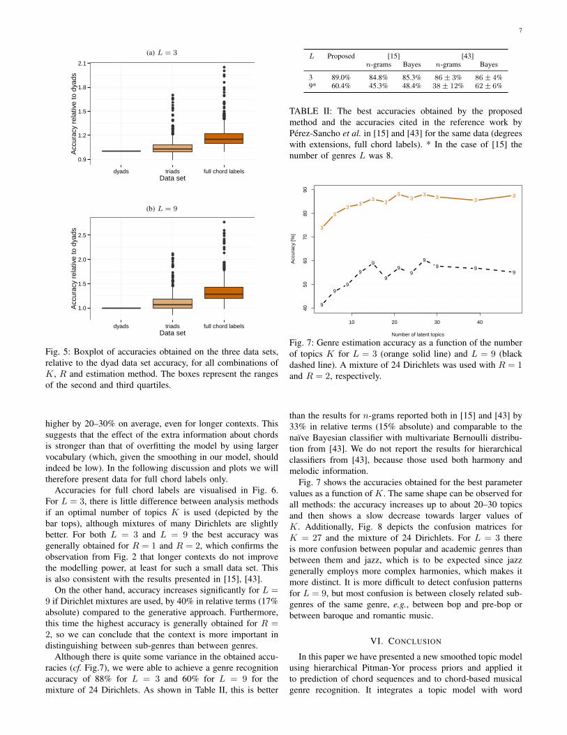
The most popular choice of a prior over categorical distribu-tions (such as the topic posteriors) is the Dirichlet distribution.However, because the topic posterior density appears to bemultimodal (see Fig. 4), we use Dirichlet mixtures [42]:

P(θs|g,Λ) =

D∑d=1

λdDir(θs;ρd), (29)

where λ are the mixing coefficients and the Dirichlets are pa-rameterised by K-element vectors ρd. The mixture coefficientsas well as the parameters of the Dirichlets can be found usingthe EM algorithm (detailed in the Appendix).

C. Results

Experiments were performed for all combinations of the pa-rameters: the number of genres and sub-genres L ∈ {3, 9}, thenumber of topics K ∈ {3, 9, 12, 15, 18, 21, 24, 27, 30, 39, 48}and the context length R ∈ {0, 1, 2, 3, }. All three chord detaillevels were used (dyads, triads, full chords) and 7 estimationmethods: generative, and Dirichlet mixtures of 1, 2, 4, 6, 12and 24 components. For every set of parameter values, topicposterior samples were collected with B1 = 500, B2 = 50and S = 100 and this was performed 20 times, resultingin 2000 topic posterior samples per song. We have used thesame division into training and test data as in the symbolicexperiments.

The accuracy of musical genre estimation was calculated asthe average over accuracies for each genre:

A =1

L

L∑g=1

NPgNTg

, (30)

where NPg is the number of correctly identified songs forgenre g and NTg is the total number of songs in that genre.

Fig. 5 shows a plot of accuracies relative to the accuracy fordyads, for all values of L, K, R and all methods. We see thathigher detail in chord descriptions translated to an accuracy

7

(a) L = 3

●●

●

●

●

●

●

●

●

●

●

●

●

●

●

●●●

●

●

●

●

●

●

●

●●

●●●

●

●●

●

●

●

●

●

●●

●

●

●

●●●

●

●

●

●

●●

●

●

●●

●●

●

●

●

●

●●

●

●

●

●●

●

0.9

1.2

1.5

1.8

2.1

dyads triads full chord labelsData set

Acc

urac

y re

lativ

e to

dya

ds

(b) L = 9

●

●

●

●

●

●

●

●●

●

●

●

●

●

●

●

●

●

●

●

●

●●

●●●

●

●

●

●●

●

●

●

●

●

●●

●

●

●

●

●●●

●

●

●●

●

●●

1.0

1.5

2.0

2.5

dyads triads full chord labelsData set

Acc

urac

y re

lativ

e to

dya

ds

Fig. 5: Boxplot of accuracies obtained on the three data sets,relative to the dyad data set accuracy, for all combinations ofK, R and estimation method. The boxes represent the rangesof the second and third quartiles.

higher by 20–30% on average, even for longer contexts. Thissuggests that the effect of the extra information about chordsis stronger than that of overfitting the model by using largervocabulary (which, given the smoothing in our model, shouldindeed be low). In the following discussion and plots we willtherefore present data for full chord labels only.

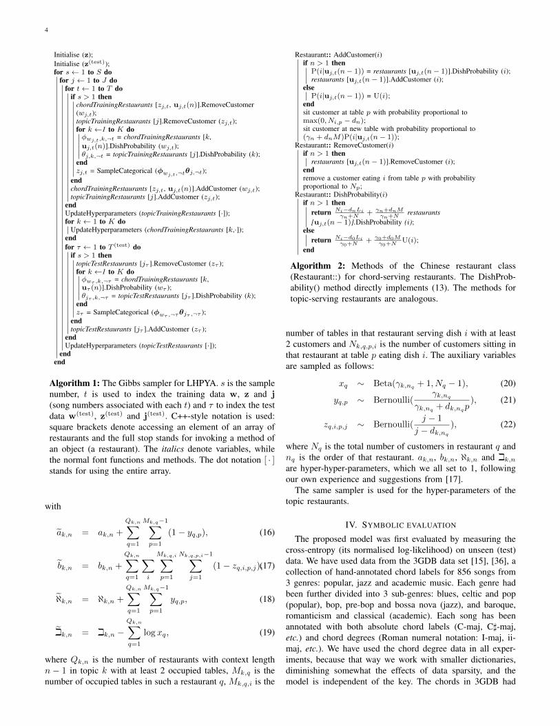
Accuracies for full chord labels are visualised in Fig. 6.For L = 3, there is little difference between analysis methodsif an optimal number of topics K is used (depicted by thebar tops), although mixtures of many Dirichlets are slightlybetter. For both L = 3 and L = 9 the best accuracy wasgenerally obtained for R = 1 and R = 2, which confirms theobservation from Fig. 2 that longer contexts do not improvethe modelling power, at least for such a small data set. Thisis also consistent with the results presented in [15], [43].

On the other hand, accuracy increases significantly for L =9 if Dirichlet mixtures are used, by 40% in relative terms (17%absolute) compared to the generative approach. Furthermore,this time the highest accuracy is generally obtained for R =2, so we can conclude that the context is more important indistinguishing between sub-genres than between genres.

Although there is quite some variance in the obtained accu-racies (cf. Fig.7), we were able to achieve a genre recognitionaccuracy of 88% for L = 3 and 60% for L = 9 for themixture of 24 Dirichlets. As shown in Table II, this is better

L Proposed [15] [43]n-grams Bayes n-grams Bayes

3 89.0% 84.8% 85.3% 86± 3% 86± 4%9* 60.4% 45.3% 48.4% 38± 12% 62± 6%

TABLE II: The best accuracies obtained by the proposedmethod and the accuracies cited in the reference work byPerez-Sancho et al. in [15] and [43] for the same data (degreeswith extensions, full chord labels). * In the case of [15] thenumber of genres L was 8.

3

33

33

3

33

3 3 33

10 20 30 40

4050

6070

8090

Number of latent topics

Acc

urac

y [%

]

9

99

9

9

9

99

99 9

9

Fig. 7: Genre estimation accuracy as a function of the numberof topics K for L = 3 (orange solid line) and L = 9 (blackdashed line). A mixture of 24 Dirichlets was used with R = 1and R = 2, respectively.

than the results for n-grams reported both in [15] and [43] by33% in relative terms (15% absolute) and comparable to thenaıve Bayesian classifier with multivariate Bernoulli distribu-tion from [43]. We do not report the results for hierarchicalclassifiers from [43], because those used both harmony andmelodic information.

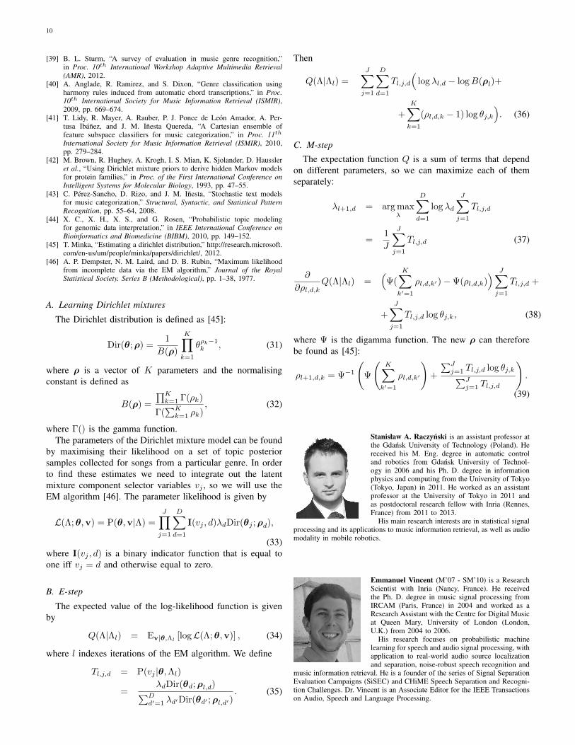
Fig. 7 shows the accuracies obtained for the best parametervalues as a function of K. The same shape can be observed forall methods: the accuracy increases up to about 20–30 topicsand then shows a slow decrease towards larger values ofK. Additionally, Fig. 8 depicts the confusion matrices forK = 27 and the mixture of 24 Dirichlets. For L = 3 thereis more confusion between popular and academic genres thanbetween them and jazz, which is to be expected since jazzgenerally employs more complex harmonies, which makes itmore distinct. It is more difficult to detect confusion patternsfor L = 9, but most confusion is between closely related sub-genres of the same genre, e.g., between bop and pre-bop orbetween baroque and romantic music.

VI. CONCLUSION

In this paper we have presented a new smoothed topic modelusing hierarchical Pitman-Yor process priors and applied itto prediction of chord sequences and to chord-based musicalgenre recognition. It integrates a topic model with word

8

(a) L = 3 (b) L = 9

Fig. 6: Accuracies obtained for all analysis methods (marked on the horizontal axis) and values of R. Bars correspond tominimal, mean and maximal values over all K’s for a particular method and value of R.

(chord) n-grams and is therefore capable of handling datafor which the bag-of-words assumption does not hold, suchas chord sequences, where progressions between chords, inaddition to the chords themselves, contribute to discriminationbetween musical genres. Using topic models is more flexiblethan the previously proposed genre-dependent n-gram modelby allowing both the songs and the genres to be mixtures oflatent topics. Of course, the proposed model is not limitedto modelling chords and it would be interesting to apply itto other musical sequences, such as pitches (e.g., melodies orvoices), rhythm, etc.

In general, this model is potentially useful in all problemswhere topic models are used and the order of words matters,e.g. in text document modelling [18] or in genomic informationanalysis [44].

REFERENCES

[1] E. Vincent, S. Raczynski, N. Ono, and S. Sagayama, “A roadmaptowards versatile MIR,” in Proc. 11th International Conference onMusic Information Retrieval (ISMIR), 2010, pp. 662–664.

[2] M. Mauch, S. Dixon, C. Harte, and Q. Mary, “Discovering chord idiomsthrough Beatles and Real Book songs,” in Proc. 8th InternationalSociety for Music Information Retrieval (ISMIR), 2007, pp. 255–258.

[3] M. Ogihara and T. Li, “N-gram chord profiles for composer stylerepresentation,” in Proc. 9th International Society for Music InformationRetrieval (ISMIR), 2008, pp. 671–676.

[4] H. Papadopoulos and G. Peeters, “Large-scale study of chord estimationalgorithms based on chroma representation and HMM,” in InternationalWorkshop on Content-Based Multimedia Indexing (CBMI). IEEE, 2007,pp. 53–60.

[5] Y. Ueda, Y. Uchiyama, T. Nishimoto, N. Ono, and S. Sagayama, “HMM-based approach for automatic chord detection using refined acousticfeatures,” in Proc. International Conference on Acoustics, Speech, andSignal Processing (ICASSP). IEEE, 2010, pp. 5518–5521.

[6] K. Lee, “A system for automatic chord transcription from audio usinggenre-specific hidden Markov models,” Adaptive Multimedial Retrieval:Retrieval, User, and Semantics, pp. 134–146, 2008.

[7] K. Yoshii and M. Goto, “Unsupervised music understanding based onnonparametric Bayesian models,” in Proc. International Conference onAcoustics, Speech and Signal Processing (ICASSP). IEEE, 2012, pp.5353–5356.

[8] S. A. Raczynski, S. Fukayama, and E. Vincent, “Melody harmonisationwith interpolated probabilistic models,” INRIA, Research Report RR-8110, October 2012. [Online]. Available: http://hal.inria.fr/hal-00742957

[9] “PG Music Inc. Band-in-a-Box,” http://www.pgmusic.com/, August2012.

[10] I. Simon, D. Morris, and S. Basu, “MySong: automatic accompanimentgeneration for vocal melodies,” in Proc. 26th SIGCHI Conference onHuman Factors in Computing Systems, 2008, pp. 725–734.

[11] S. Fukayama, K. Nakatsuma, S. Sako, T. Nishimoto, and S. Sagayama,“Automatic song composition from the lyrics exploiting prosody ofthe Japanese language,” in Proc. 7th Sound and Music ComputingConference (SMC), 2010, pp. 299–302.

[12] G. Sargent, F. Bimbot, and E. Vincent, “A regularity-constrained Viterbialgorithm and its application to the structural segmentation of songs,”in Proc. 12th International Society for Music Information Retrieval(ISMIR), 2011, pp. 483–488.

[13] M. Mauch, K. Noland, and S. Dixon, “Using musical structure to

9

(a) L = 3, R = 1, K = 27, 24 Dirichlets

Pop

ular

Jazz

Aca

dem

ic

Academic

Jazz

Popular

11%

4%

80%

7%

83%

9%

82%

12%

11%

Predicted genre

Act

ual g

enre

(b) L = 9, R = 2, K = 27, 24 Dirichlets

Pop

Blu

es

Cel

tic

Bop

Bos

sano

va

Pre

bop

Rom

antic

ism

Cla

ssic

al

Bar

oque

Baroque

Classical

Romanticism

Prebop

Bossanova

Bop

Celtic

Blues

Pop

6%

6%

0%

4%

18%

15%

30%

24%

43%

0%

10%

0%

0%

0%

0%

19%

36%

7%

16%

10%

2%

3%

3%

2%

38%

28%

29%

18%

2%

7%

15%

27%

45%

8%

0%

4%

2%

0%

0%

7%

9%

2%

0%

0%

0%

10%

2%

7%

65%

21%

21%

0%

0%

0%

6%

18%

81%

2%

3%

11%

5%

4%

7%

4%

36%

2%

0%

3%

0%

2%

8%

11%

38%

16%

0%

3%

15%

4%

0%

0%

0%

Predicted genre

Act

ual g

enre

Fig. 8: Confusion matrices for best sets of parameters. Shadescorrespond to absolute counts of labelling an “actual genre”as a “predicted count”. Marginal barplots show total countsfor the actual and predicted genres. Additionally, the textlabels show counts relative to the total number of songs for aparticular actual genre (i.e., rows sum up to one)

enhance automatic chord transcription,” in Proc. 10th InternationalSociety for Music Information Retrieval (ISMIR), 2009, pp. 231–236.

[14] S. A. Raczynski and E. Vincent, “Dynamic Bayesian networks forsymbolic polyphonic pitch modeling,” IEEE Transactions on Audio,Speech and Language Processing, 2013.

[15] C. Perez-Sancho, D. Rizo, and J. M. Inesta, “Genre classification usingchords and stochastic language models,” Connection science, vol. 21,no. 2-3, pp. 145–159, 2009.

[16] D. M. Blei, A. Y. Ng, and M. I. Jordan, “Latent Dirichlet allocation,”Journal of Machine Learning Research, vol. 3, pp. 993–1022, 2003.

[17] I. Sato and H. Nakagawa, “Topic models with power-law using Pitman-Yor process,” in Proc. 16th ACM SIGKDD International Conference onKnowledge Discovery and Data Mining, 2010, pp. 673–681.

[18] H. M. Wallach, “Topic modeling: beyond bag-of-words,” in Proc. 23rdInternational Conference on Machine Learning. ACM, 2006, pp. 977–984.

[19] D. J. Hu and L. K. Saul, “A probabilistic topic model for unsupervisedlearning of musical key-profiles,” in Proc. 10th International Societyfor Music Information Retrieval (ISMIR), 2009, pp. 441–446.

[20] A. Spiliopoulou and A. Storkey, “A Topic Model for Melodic Se-quences,” ArXiv e-prints, Jun. 2012.

[21] R. Scholz, E. Vincent, and F. Bimbot, “Robust modeling of musicalchord sequences using probabilistic N -grams,” in Proc. InternationalConference on Acoustics, Speech and Signal Processing (ICASSP).IEEE, 2009, pp. 53–56.

[22] S. F. Chen and J. Goodman, “An empirical study of smoothing tech-niques for language modeling,” in Proc. 34th annual meeting onAssociation for Computational Linguistics. ACL, 1996, pp. 310–318.

[23] T. Hofmann, “Probabilistic latent semantic indexing,” in Proc. 22ndACM SIGIR Conference on Research and Development in InformationRetrieval. ACM, 1999, pp. 50–57.

[24] C. Zhai and J. Lafferty, “A study of smoothing methods for languagemodels applied to ad hoc information retrieval,” in Proc. 24th ACM SI-GIR Conference on Research and Development in Information Retrieval.ACM, 2001, pp. 334–342.

[25] R. Kneser and H. Ney, “Improved backing-off for m-gram languagemodeling,” in Proc. International Conference on Acoustics, Speech, andSignal Processing (ICASSP), vol. 1. IEEE, 1995, pp. 181–184.

[26] Y. W. Teh, M. I. Jordan, M. J. Beal, and D. M. Blei, “HierarchicalDirichlet processes,” Journal of the American Statistical Association,vol. 101, no. 476, pp. 1566–1581, 2006.

[27] Y. W. Teh, “A hierarchical Bayesian language model based on Pitman-Yor processes,” in Proc. 21st International Conference on Computa-tional Linguistics and the 44th annual meeting of the Association forComputational Linguistics. ACL, 2006, pp. 985–992.

[28] M. Kaban and G. Ata, “Simplicial mixtures of markov chains: Dis-tributed modelling of dynamic user profiles,” Advances in neural infor-mation processing systems, vol. 16, p. 9, 2004.

[29] D. J. C. MacKay and L. C. B. Peto, “A hierarchical Dirichlet languagemodel,” Natural Language Engineering, vol. 1, no. 3, pp. 1–19, 1995.

[30] Y. W. Teh, “A Bayesian interpretation of interpolated Kneser-Ney,”National University of Singapore, School of Computing, Tech. Rep.,2006.

[31] T. L. Griffiths and M. Steyvers, “Finding scientific topics,” in Pro-ceedings of the National Academy of Sciences of the United States ofAmerica, vol. 101 (Suppl 1), 2004, pp. 5228–5235.

[32] H. M. Wallach, I. Murray, R. Salakhutdinov, and D. Mimno, “Evaluationmethods for topic models,” in Proc. 26th International Conference onMachine Learning. ACM, 2009, pp. 1105–1112.

[33] J. Pitman, “Combinatorial stochastic processes,” University of CaliforniaBerkeley, Dept. Statistics, Tech. Rep. 621, 2002.

[34] D. M. Griffiths, T. L. Blei, M. Tenenbaum, and J. B. Jordan, “Hierarchi-cal topic models and the nested Chinese restaurant process,” in Advancesin Neural Information Processing Systems (NIPS). MIT Press, 2004.

[35] H. M. Wallach, C. Sutton, and A. McCallum, “Bayesian modelingof dependency trees using hierarchical Pitman-Yor priors,” in ICMLWorkshop on Prior Knowledge for Text and Language Processing, 2008,pp. 15–20.

[36] “3 Genre Database (3GDB),” http://grfia.dlsi.ua.es/cm/projects/prosemus/database.php, February 2013.

[37] M. A. Newton and A. E. Raftery, “Approximate Bayesian inferencewith the weighted likelihood bootstrap,” Journal of the Royal StatisticalSociety. Series B (Methodological), pp. 3–48, 1994.

[38] N. Scaringella, G. Zoia, and D. Mlynek, “Automatic genre classificationof music content: a survey,” IEEE Signal Processing Magazine, vol. 23,no. 2, pp. 133–141, 2006.

10

[39] B. L. Sturm, “A survey of evaluation in music genre recognition,”in Proc. 10th International Workshop Adaptive Multimedia Retrieval(AMR), 2012.

[40] A. Anglade, R. Ramirez, and S. Dixon, “Genre classification usingharmony rules induced from automatic chord transcriptions,” in Proc.10th International Society for Music Information Retrieval (ISMIR),2009, pp. 669–674.

[41] T. Lidy, R. Mayer, A. Rauber, P. J. Ponce de Leon Amador, A. Per-tusa Ibanez, and J. M. Inesta Quereda, “A Cartesian ensemble offeature subspace classifiers for music categorization,” in Proc. 11thInternational Society for Music Information Retrieval (ISMIR), 2010,pp. 279–284.

[42] M. Brown, R. Hughey, A. Krogh, I. S. Mian, K. Sjolander, D. Haussleret al., “Using Dirichlet mixture priors to derive hidden Markov modelsfor protein families,” in Proc. of the First International Conference onIntelligent Systems for Molecular Biology, 1993, pp. 47–55.

[43] C. Perez-Sancho, D. Rizo, and J. M. Inesta, “Stochastic text modelsfor music categorization,” Structural, Syntactic, and Statistical PatternRecognition, pp. 55–64, 2008.

[44] X. C., X. H., X. S., and G. Rosen, “Probabilistic topic modelingfor genomic data interpretation,” in IEEE International Conference onBioinformatics and Biomedicine (BIBM), 2010, pp. 149–152.

[45] T. Minka, “Estimating a dirichlet distribution,” http://research.microsoft.com/en-us/um/people/minka/papers/dirichlet/, 2012.

[46] A. P. Dempster, N. M. Laird, and D. B. Rubin, “Maximum likelihoodfrom incomplete data via the EM algorithm,” Journal of the RoyalStatistical Society. Series B (Methodological), pp. 1–38, 1977.

A. Learning Dirichlet mixtures

The Dirichlet distribution is defined as [45]:

Dir(θ;ρ) =1

B(ρ)

K∏k=1

θρk−1k , (31)

where ρ is a vector of K parameters and the normalisingconstant is defined as

B(ρ) =

∏Kk=1 Γ(ρk)

Γ(∑Kk=1 ρk)

, (32)

where Γ() is the gamma function.The parameters of the Dirichlet mixture model can be found

by maximising their likelihood on a set of topic posteriorsamples collected for songs from a particular genre. In orderto find these estimates we need to integrate out the latentmixture component selector variables vj , so we will use theEM algorithm [46]. The parameter likelihood is given by

L(Λ;θ,v) = P(θ,v|Λ) =

J∏j=1

D∑d=1

I(vj , d)λdDir(θj ;ρd),

(33)where I(vj , d) is a binary indicator function that is equal toone iff vj = d and otherwise equal to zero.

B. E-step

The expected value of the log-likelihood function is givenby

Q(Λ|Λl) = Ev|θ,Λl [logL(Λ;θ,v)] , (34)

where l indexes iterations of the EM algorithm. We define

Tl,j,d = P(vj |θ,Λl)

=λdDir(θd;ρl,d)∑D

d′=1 λd′Dir(θd′ ;ρl,d′). (35)

Then

Q(Λ|Λl) =

J∑j=1

D∑d=1

Tl,j,d

(log λl,d − logB(ρl)+

+

K∑k=1

(ρl,d,k − 1) log θj,k

). (36)

C. M-step

The expectation function Q is a sum of terms that dependon different parameters, so we can maximize each of themseparately:

λl+1,d = arg maxλ

D∑d=1

log λd

J∑j=1

Tl,j,d

=1

J

J∑j=1

Tl,j,d (37)

∂

∂ρl,d,kQ(Λ|Λl) =

(Ψ(

K∑k′=1

ρl,d,k′)−Ψ(ρl,d,k)) J∑j=1

Tl,j,d +

+

J∑j=1

Tl,j,d log θj,k, (38)

where Ψ is the digamma function. The new ρ can thereforebe found as [45]:

ρl+1,d,k = Ψ−1

(Ψ

(K∑k′=1

ρl,d,k′

)+

∑Jj=1 Tl,j,d log θj,k∑J

j=1 Tl,j,d

).

(39)

Stanisław A. Raczynski is an assistant professor atthe Gdansk University of Technology (Poland). Hereceived his M. Eng. degree in automatic controland robotics from Gdansk University of Technol-ogy in 2006 and his Ph. D. degree in informationphysics and computing from the University of Tokyo(Tokyo, Japan) in 2011. He worked as an assistantprofessor at the University of Tokyo in 2011 andas postdoctoral research fellow with Inria (Rennes,France) from 2011 to 2013.

His main research interests are in statistical signalprocessing and its applications to music information retrieval, as well as audiomodality in mobile robotics.

Emmanuel Vincent (M’07 - SM’10) is a ResearchScientist with Inria (Nancy, France). He receivedthe Ph. D. degree in music signal processing fromIRCAM (Paris, France) in 2004 and worked as aResearch Assistant with the Centre for Digital Musicat Queen Mary, University of London (London,U.K.) from 2004 to 2006.

His research focuses on probabilistic machinelearning for speech and audio signal processing, withapplication to real-world audio source localizationand separation, noise-robust speech recognition and

music information retrieval. He is a founder of the series of Signal SeparationEvaluation Campaigns (SiSEC) and CHiME Speech Separation and Recogni-tion Challenges. Dr. Vincent is an Associate Editor for the IEEE Transactionson Audio, Speech and Language Processing.