Genomic prediction for additive and dominance effects of ... · proposed was the GBLUP-D, which...

Genetics and Molecular Research 15 (4): gmr15048764

Genomic prediction for additive and dominance effects of censored traits in pigs

V.S. Santos1, S. Martins Filho1, M.D.V. Resende2, C.F. Azevedo1, P.S. Lopes3, S.E.F. Guimarães3 and F.F. Silva3

1Departamento de Estatística, Universidade Federal de Viçosa, Viçosa, MG, Brasil2Empresa Brasileira de Pesquisa Agropecuária, Centro Nacional de Pesquisa de Florestas, Colombo, PR, Brasil3Departamento de Zootecnia, Universidade Federal de Viçosa, Viçosa, MG, Brasil

Corresponding author: V.S. SantosE-mail: [email protected]

Genet. Mol. Res. 15 (4): gmr15048764Received May 5, 2016Accepted August 30, 2016Published October 17, 2016DOI http://dx.doi.org/10.4238/gmr15048764

Copyright © 2016 The Authors. This is an open-access article distributed under the terms of the Creative Commons Attribution ShareAlike (CC BY-SA) 4.0 License.

ABSTRACT. Age at the time of slaughter is a commonly used trait in animal breeding programs. Since studying this trait involves incomplete observations (censoring), analysis can be performed using survival models or modified linear models, for example, by sampling censored data from truncated normal distributions. For genomic selection, the greatest genetic gains can be achieved by including non-additive genetic effects like dominance. Thus, censored traits with effects on both survival models have not yet been studied under a genomic selection approach. We aimed to predict genomic values using the Cox model with dominance effects and compare these results with the linear model with and without censoring. Linear models were fitted via the maximum likelihood method. For censored data, sampling through

2V.S. Santos et al.


the truncated normal distribution was used, and the model was called the truncated normal linear via Gibbs sampling (TNL). We used an F2 pig population; the response variable was time (days) from birth to slaughter. Data were previously adjusted for fixed effects of sex and contemporary group. The model predictive ability was calculated based on correlation of predicted genomic values with adjusted phenotypic values. The results showed that both with and without censoring, there was high agreement between Cox and linear models in selection of individuals and markers. Despite including the dominance effect, there was no increase in predictive ability. This study showed, for the first time, the possibility of performing genomic prediction of traits with censored records while using the Cox survival model with additive and dominance effects.

Key words: GBLUP; Censored data; Mixed model; Survival models

INTRODUCTION

Genomic selection (GS) in pigs has been performed mainly for traits of economic importance, for those related to growth and reproduction, and also for carcass traits. However, GS can also be applied toward traits such as age at slaughter, which is defined as the length of productive life (for instance, the time in days from birth to slaughter). Since this involves the presence of incomplete observations (i.e., censored data), not all individuals have achieved the desired slaughter weight, and the analysis of this trait can be performed by means of survival analysis models or different modifications of the linear model (Serenius et al., 2006; Hou et al., 2009).

In animal breeding, Weibul and Cox (Cox, 1972) survival models have been fitted using the Survival Kit software (Ducrocq et al., 2010), which only estimates the additive effects based on pedigree using the Bayesian approach.

In the context of GS, Santos et al. (2015) were the pioneers when it came to performing the genomic prediction of censored phenotypes while using the Cox survival model. As such, the model with only additive effects was considered, and was fitted by using the coxme function of the R software, since the relationship matrix based on pedigree was replaced by the relationship matrix based on markers. Furthermore, in GS, Kärkkäinen and Sillanpaa (2013) proposed the use of Bayesian threshold models for data in binary and ordinal scale in order to evaluate censored traits.

Recently, non-additive effects such as dominance have been included in the GS of pigs (Su et al., 2012; Costa et al., 2015). This effect is defined as the interaction between alleles at the same locus, and it is expected that the inclusion of this effect in genomic models will increase prediction accuracy (Su et al., 2012).

To study additive and non-additive effects in GS, the method that was originally proposed was the GBLUP-D, which consists of replacing additive and dominance genomic relationship matrices based on pedigree with marker-based relationship matrices. Besides the GBLUP-D, other methods such as LASSO, Ridge, and Bayesian (Bayes, Bayes B, t-BLASSO) were proposed for additive-dominance genomic models (Azevedo et al., 2015).

However, no study was performed based on survival models considering both effects

3Genomic additive and dominance variance of censored traits


(additive and dominance) so much by usual analysis based on pedigree by genomic selection. Thus, we aimed to build upon the method proposed by Santos et al. (2015) to include dominance effects and evaluate their performance. In addition, we also aimed to compare the proposed model with alternative linear models in the presence and absence of censored observations.

MATERIAL AND METHODS

Population establishment and the phenotypic measurements were performed at the Pig Breeding Farm of the Department of Animal Science, Universidade Federal de Viçosa (UFV), MG, Brazil. The phenotypic data consisted of an F2 population that was generated by crossing 11 boars and 54 dams that were randomly selected from the F1 generation, which was initially created by crossing two native Brazilian Piau boars with 18 commercial sows (Landrace x Large White x Pietrain). The use of these animals was reviewed and approved by the Bioethics committee of the Department of Veterinary Medicine (UFV) in agreement with the Guide to the Care and Use of Experimental Animals of the Canadian Council on Animal Care.

DNA was extracted from the white blood cells of parental, F1, and F2 animals at the Animal Biotechnology Laboratory of the Animal Science Department of the Universidade Federal de Viçosa. More details can be found in Band et al. (2005). From the F2 population, 345 animals were genotyped for 384 single nucleotide polymorphisms (SNPs). The low-density customized SNPChip used was based on the Illumina Porcine SNP60 BeadChip.

These SNPs were selected according to QTL positions that were previously identified in this population using meta-analyses and fine mapping (Verardo et al., 2015). Therefore, although a small number of markers were used, the customized SNPchip based on previously identified QTL positions ensures appropriate coverage of the relevant genome regions in this population. From these, 66 SNPs were discarded because of a low-genotyping call rate (< 0.95), and from the remaining 318 SNPs, 81 were discarded due to a minor allele frequency <0.05. Thus, 237 SNP markers were distributed on the Sus scrofa chromosomes (SSC) as follows: SSC1 (N = 56), SSC4 (N = 54), SSC7 (N = 59), SSC8 (N = 31), SSC17 (N = 25), and SSCX (N = 12).

In order to identify individuals with rapid weight gain for slaughter, the time in days from birth until the slaughter of the animal was considered a response variable. The desired weight of the animals at the time of slaughter in this population was around 65 kg (Band et al., 2005). The exact time it took an animal to gain the desired weight was not known, as daily weighing was impractical. Only the ages and weights of the animals at the time of slaughter were known.

As a result, censoring was created based on slaughter weight, i.e., animals that did not reach 65 kg were referred to as censored (event = 0), whereas animals that reached that weight or more were referred to as a failure (event = 1). In this dataset, the proportion of censoring was around 0.561, i.e., about 44% of the animals weighed at least 65 kg. The data used in the analysis was adjusted for the fixed effects of sex and contemporary group (Silva et al., 2013), and the halothane gene was included as an additional marker.

Statistical models

The models shown in Table 1 were fitted to compare estimates of variance components and predicted genetic values using linear and survival models, with and without the effects of dominance and censoring.

4V.S. Santos et al.


According to Schaeffer (2013), there are three possible situations for the analysis of censored data: 1) when the censoring is removed in the analysis; 2) when the censoring is included in the analysis, but is not properly taken into account, or 3) when the censoring is included in the analysis and is properly taken into account. Additive linear (AL), additive-dominance linear via ML (ADL), additive uncensored Cox (AUC), and additive-dominance uncensored Cox (ADUC) models belong to situation 2 and additive truncated normal linear (ATNL), additive-dominance truncated normal linear (ADTNL), additive Cox (AC), and additive-dominance Cox (ADC) models to situation 3. In the ATNL and ADTNL models, the censored records were simulated from truncated normal distributions (Pérez and de los Campos, 2014).

AL and ADL models

The AL and ADL models were fitted using the lmekin function of the coxme package (Therneau, 2012) of the R software (R Development Core Team, 2016). The linear mixed model with only additive effects (AL) was defined as follows:

Table 1. Evaluated models for time in days from birth to slaughter of the animal, considering censoring and additive and dominance effects.

Models Additive effect Additive and dominance effect Uncensored Additive linear (AL) Additive-dominance linear via ML (ADL)

Additive uncensored Cox (AUC) Additive-dominance uncensored Cox (ADUC) Censored Additive truncated normal linear (ATNL) Additive-dominance truncated normal linear (ADTNL)

Additive Cox (AC) Additive-dominance Cox (ADC)

1y Za eµ= =+ + (Equation 1)

where y is a vector of length n of adjusted phenotypes for fixed effects of sex and contemporary group, ignoring censoring; µ is an intercept; a is the vector of random additive effects of individuals; Z is the incidence matrix for the random effects; and e is the vector of errors assumed as 2(0, )eN Iσ . The additive random effect was assumed to be 2(0, )aN Gσ , where G is the additive genomic relationship matrix given by VanRaden (2008):

( )1

'

2m

j jj

WWGp q

=

=

∑(Equation 2)

where W has the dimension of the number of animals (n) by the number of loci (m), with elements that are equal to -2pj, 1-2pj, and 2-2pj for the genotypes mm, Mm, and MM, respectively; pj is the allelic frequency of M at locus j and qj = 1- pj.

The lmekin function does not allow for the prediction of two separate random effects. Thus, the linear mixed model with additive and dominance effects (ADL) was defined as follows:



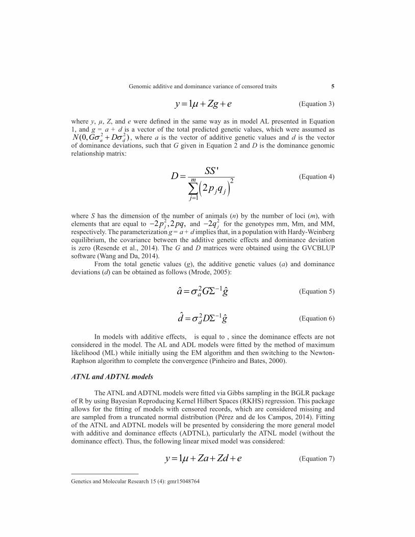
where y, µ, Z, and e were defined in the same way as in model AL presented in Equation 1, and g = a + d is a vector of the total predicted genetic values, which were assumed as

2 2(0, )a dN G Dσ σ+ , where a is the vector of additive genetic values and d is the vector of dominance deviations, such that G given in Equation 2 and D is the dominance genomic relationship matrix:

1y Zg eµ= + + (Equation 3)

( )21

'

2m

j jj

SSDp q

=

=∑

(Equation 4)

where S has the dimension of the number of animals (n) by the number of loci (m), with elements that are equal to 22 , 2 ,jp pq− and 22 jq− for the genotypes mm, Mm, and MM, respectively. The parameterization g = a + d implies that, in a population with Hardy-Weinberg equilibrium, the covariance between the additive genetic effects and dominance deviation is zero (Resende et al., 2014). The G and D matrices were obtained using the GVCBLUP software (Wang and Da, 2014).

From the total genetic values (g), the additive genetic values (a) and dominance deviations (d) can be obtained as follows (Mrode, 2005):

2 1ˆ ˆaa G gσ −= Σ (Equation 5)

2 1ˆ ˆdd D gσ −= Σ (Equation 6)

In models with additive effects, is equal to , since the dominance effects are not considered in the model. The AL and ADL models were fitted by the method of maximum likelihood (ML) while initially using the EM algorithm and then switching to the Newton-Raphson algorithm to complete the convergence (Pinheiro and Bates, 2000).

ATNL and ADTNL models

The ATNL and ADTNL models were fitted via Gibbs sampling in the BGLR package of R by using Bayesian Reproducing Kernel Hilbert Spaces (RKHS) regression. This package allows for the fitting of models with censored records, which are considered missing and are sampled from a truncated normal distribution (Pérez and de los Campos, 2014). Fitting of the ATNL and ADTNL models will be presented by considering the more general model with additive and dominance effects (ADTNL), particularly the ATNL model (without the dominance effect). Thus, the following linear mixed model was considered:

1y Za Zd eµ= + + + (Equation 7)

6V.S. Santos et al.


where µ, Z, and e are defined as in the AL and ADL models, a is the vector of additive genetic values, and d is the vector of dominance deviations. The above model induces the conditional distribution:

( )2| , ey N Za Zd Iθ µ σ+ + (Equation 8)

where θ represents the set of unknown parameters µ, a, d, 2aσ , 2

dσ , and 2eσ . For µ, a, and d,

the following prior distributions were assumed:

2 2 2 21 1 2, 2( ) tan ; | , (0, ) | (0, )a a d dp cons t a K N K and d K N Kµ σ σ σ σ∝ ∼ ∼ (Equation 9)

where K1 and K2 are the kernel square matrices with a size equal to the number of individuals, and in the ADTNL model, K1 and K2 were replaced by the additive (G) and dominance (D) genomic relationship matrices (de Los Campos et al., 2009). For variance components 2

aσ , 2dσ ,

and 2eσ were assumed weak priors. The vector of phenotypes includes censored and uncensored

records. Thus, the density function of the conditional distribution in (8) is given by

( )' '2/22 ' '

121 1

1( | ) (2 ) exp2

i i ie i i

i i ee

t z a z dp y x Yobs z a z d xµ

µ

µ

η ηη

ηθ πσ φ

σσ−

= = +

− −∝ − − −∑ ∏ (Equation 10)

where Yobs is the dataset with uncensored records of dimension nu, n is the total number of observations, Φ is the cumulative distribution function of the standard normal, and ti is the truncation point, which was 150 days in this study.

By using a data augmentation technique for censored observations, the conditional distribution of the observed data in Equation 8 can be rewritten as:

( ) ( )2 2/22 ' ' ' ' ' '2

1 1

1( | ) (2 ) exp2 iie ceni i i i i iobs

i iep y x y x z a z d y x z a z d

µ

µ

η ηη

ηθ πσ β β

σ−

= = +

∝ − − − − + − − −∑ ∑ (Equation 11)

where icen iy t≥ , i.e., the unobserved value, must be greater or equal to the truncation point.

For more details, see Sorensen et al. (1998) and Guo et al. (2001). For parameter estimation, the Gibbs sampler algorithm was used while assuming 120,000 iterations. The first 20,000 iterations were discarded and, to ensure independence, a spacing of 10 between samples was considered. The convergence was verified by the Geweke criterion in the BOA package of the R software (Smith, 2007).

AC and ADC models

In the context of GS, the additive Cox model (AC) is defined as follows:

( ) { }0( )exph t h t Za= (Equation 12)



where h0(t) is an unspecified nonnegative function of time called the baseline hazard, Z is the incidence matrix for random effects, and a is the vector of additive genetic effects, which were assumed with a zero mean and variance-covariance matrix 2

1 aGσΣ = , where 2aσ is the additive

genetic variance and G is the additive genomic relationship matrix given in Equation 2.When extending the AC model presented in Equation 12, the Cox model with additive

and dominance effects (ADC) was defined as follows:

{ }0( ) h ( )exph t t Zg= (Equation 13)

where h0(t) is defined as in Equation 12 and Z is the incidence matrix of the total genetic effects (g), where g = a + d is a vector of total predicted genetic values, as in Equation 3, with zero for the mean and a variance-covariance matrix of 2 2

2 a dG Dσ σΣ = + . G and D matrices are given in Equations 2 and 4, respectively. Similar to the ADL model, the a and d random effects were considered to be independent. The individual additive genetic values (a) and dominance deviations (d) were obtained from Equations 5 and 6, respectively.

Unlike the linear model, in the Cox model, the intercept is absorbed in the baseline hazard function. In the Cox mixed model fitted with the coxme package, the estimation is based on a penalized partial likelihood that was developed by applying the Laplace approximation to the marginal likelihood function, since the solution of the multidimensional integral is intractable (Pankratz et al., 2005).

AUC and ADUC models

In order to compare the linear and Cox models in equivalent situations (normal data and uncensored), the uncensored Cox models with additive (AUC) and additive-dominance (ADUC) effects were also fitted. The difference between these models, when compared to the AC and ADC models, is that the observed time for all individuals was regarded as failure time (indicator variable of censoring equal to 1). The AC, AUC, ADC, and ADUC models were fitted by the method of ML, which was implemented in the coxme package of R (Therneau, 2012). For the Cox model, the coxme function provides only ML estimates. Thus, in order to compare the estimates that were obtained in the Cox model without censoring with estimates obtained from the linear model, we used the method ML and not REML for linear models.

Additive ˆ a(m ) and dominance ˆ d(m ) markers effect estimates

The ˆ am and ˆ dm effects were obtained from their respective expressions (Resende et al., 2014):

1ˆ ˆ( ' ) 'am W W W a−= (Equation 14)

where a and d are the vectors of additive genetic values and dominance deviations in each model, and W and S are the matrices that were previously defined.

1 ˆˆ ( ' ) 'dm S S S d−= (Equation 15)

8V.S. Santos et al.


Heritability estimates

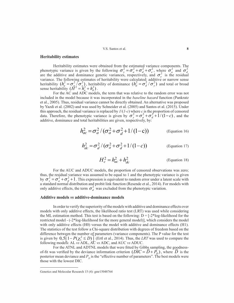
Heritability estimates were obtained from the estimated variance components. The phenotypic variance is given by the following 2 2 2 2

y a d eσ σ σ σ= + + , where 2aσ and 2

dσ are the additive and dominance genetic variances, respectively, and 2

eσ is the residual variance. The following estimates of heritability were calculated: additive or narrow sense heritability 2 2 2( / )a a yh σ σ= , heritability of dominance 2 2 2( / )d d yh σ σ= and total or broad sense heritability 2 2 2( )a dH h h= + .

For the AC and ADC models, the term that was relative to the random error was not included in the model because it was incorporated in the baseline hazard function (Pankratz et al., 2005). Thus, residual variance cannot be directly obtained. An alternative was proposed by Yazdi et al. (2002) and was used by Schneider et al. (2005) and Santos et al. (2015). Under this approach, the residual variance is replaced by 1/(1-c) where c is the proportion of censored data. Therefore, the phenotypic variance is given by 2 2 2 1/ (1 )y a d cσ σ σ= + + − , and the additive, dominance and total heritabilities are given, respectively, by:

2 2 2 2/ ( 1/ (1 c))ac a a dh σ σ σ= + + − (Equation 16)

For the AUC and ADUC models, the proportion of censored observations was zero; thus, the residual variance was assumed to be equal to 1 and the phenotypic variance is given by 2 2 2 1y a dσ σ σ= + + . This expression is equivalent to random error under a latent scale with a standard normal distribution and probit link function (Resende et al., 2014). For models with only additive effects, the term 2

dσ was excluded from the phenotypic variation.

Additive models vs additive-dominance models

In order to verify the superiority of the models with additive and dominance effects over models with only additive effects, the likelihood ratio test (LRT) was used while considering the ML estimation method. This test is based on the following: D = [-2*log-likelihood for the restricted model - (-2*log-likelihood for the more general model)], which considers the model with only additive effects (H0) versus the model with additive and dominance effects (H1). The statistics of the test follow a Chi-square distribution with degrees of freedom based on the difference between the number of parameters (variance components). The P value for the test is given by 2

10,5 1 ( )P Dχ − ≤ (Ertl et al., 2014). Thus, the LRT was used to compare the following models: AL vs ADL, AC vs ADC, and AUC vs ADUC.

For the ATNL and ADTNL models that were fitted by Gibbs sampling, the goodness-of-fit was verified by the deviance information criterion ( )DDIC D P= + , where D is the posterior mean deviance and PD is the “effective number of parameters”. The best models were those with the lowest DIC.

2 2 2 2/ ( 1/ (1 ))adc d dh cσ σ σ= + + − (Equation 17)

(Equation 18)2 2 2c ac dcH h h= +



Model comparison

The predicted genomic values in the AC and ADC models are inversely proportional to the observed values and to the predicted genomic values in the additive and additive-dominance linear models. This is because in the Cox model, the predicted values are determined while using the hazard scale, whereas the observed data and the predicted values in the linear models are determined on the observed scale of days (Hou et al., 2009). Thus, the correlation was obtained between the ranks of sorted genomic breeding values (GBVs) in decreasing order for the Cox model, and in ascending order for the observed values and predicted GBVs in the linear models. The same idea was used for the predicted total genomic values (TGVs) with additive-dominance models. In addition, Spearman correlations between the predicted GBVs and TGVs in the eight models were also calculated. To verify whether the estimates differ from zero, Spearman’s rho was used to estimate a rank-based measure of association, with P values computed via the asymptotic t approximation.

In the Cox models (AUC and ADUC) and in the linear models fitted via ML (AL and ADL), censoring was not taken into account, i.e., the time of all individuals was considered to be failure time. This procedure was used to evaluate the prediction consistency. Similar comparisons were performed for the ATNL and ADTNL model with the AC and ADC model with censored data.

The equivalence between the Cox model and linear model when selecting the best individuals and the largest marker effects was evaluated by means of the agreement rates between the 10% largest predicted GBVs in similar additive models (AL and AUC, ATNL, and AC) and between the 10% largest predicted TGVs in the additive-dominance models (ADL and ADUC, ADTNL, and ADC). The same agreement rates were calculated for the 10% highest additive and dominance marker effects. In linear models, the selected animals were those whose genomic genetic values minimized the time until slaughter. In the Cox model, the selected animals were those whose genomic genetic values maximized the hazard (Hou et al., 2009; Sobczyńska and Blicharski, 2015).

In addition to calculating the agreement rates between models, the Cohen’s kappa coefficient (k) was obtained, which assessed the degree of agreement between two models in the above-described equivalent situations. The statistical significance of k was assessed.

RESULTS

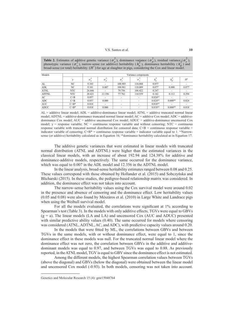
For ATNL and ADTNL models fitted via Gibbs sampling, the P values that were obtained for the Geweke criterion were higher than the predetermined significance level of 5%, thereby indicating that convergence was attained for the MCMC chain. For linear (ADL) and Cox (ADC and ADUC) models, the dominance variance was null, and on occasion the dominance heritabilities were also null (Table 2). For the ADTNL model fitted via RKHS, the dominance variance was equal to 12.36. When including the dominance effect in this model, the additive genetic variance decreased, and 11.2% of the phenotypic variation was explained by the dominance variation. Su et al. (2012), when evaluating the daily gain in Danish Duroc pigs by means of the linear model, reported dominance values explaining 5.6% of the phenotypic variation.

10V.S. Santos et al.


The additive genetic variances that were estimated in linear models with truncated normal distribution (ATNL and ADTNL) were higher than the estimated variances in the classical linear models, with an increase of about 192.94 and 124.38% for additive and dominance-additive models, respectively. The same occurred for the dominance variance, which was equal to 0.007 in the ADL model and 12.356 in the ADTNL model.

In the linear analysis, broad-sense heritability estimates ranged between 0.08 and 0.25. These values correspond with those obtained by Hollander et al. (2015) and Sobczyńska and Blicharski (2015). In these studies, the pedigree-based relationship matrix was considered. In addition, the dominance effect was not taken into account.

The narrow-sense heritability values using the Cox survival model were around 0.02 in the presence and absence of censoring and the dominance effect. Low heritability values (0.05 and 0.08) were also found by Mészáros et al. (2010) in Large White and Landrace pigs when using the Weibull survival model.

For all the models evaluated, the correlations were significant at 1% according to Spearman’s test (Table 3). In the models with only additive effects, TGVs were equal to GBVs (g = a). The linear models (LA and LA) and uncensored Cox (AUC and ADUC) presented with similar predictive ability values (0.40). The same occurred for models where censoring was considered (ATNL, ADTNL, AC, and ADC), with predictive capacity values around 0.20.

In the models that were fitted by ML, the correlations between GBVs and between TGVs in the same models, with or without dominance effect, were equal to 1, since the dominance effect in these models was null. For the truncated normal linear model where the dominance effect was not zero, the correlation between GBVs in the additive and additive-dominant models was equal to 0.97, and between TGVs was equal to 0.88. As previously reported, in the ATNL model, TGV is equal to GBV since the dominance effect is not estimated.

Among the different models, the highest Spearman correlation values between TGVs (above the diagonal) and GBVs (below the diagonal) were obtained between the linear model and uncensored Cox model (-0.93). In both models, censoring was not taken into account.

Table 2. Estimates of additive genetic variance ( 2aσ ), dominance variance ( 2

dσ ), residual variance ( 2eσ ),

phenotypic variance ( 2yσ ), narrow-sense (or additive) heritability ( 2

ah ), dominance heritability ( 2dh ) and

broad-sense (or total) heritability 2( )H for age at slaughter in pigs, considering the Cox and linear model.

Models Variance components

y 2a 2

d 2e 2

y 2ah 2

dh H2

AL NC 9.103 - 108.985 118.088 0.077 - - ADL NC 9.101 0.007 108.981 118.089 0.077 0.000 0.077 ATNL NTC 26.666 - 79.756 106.422 0.247 - - ADTNL NTC 20.421 12.356 77.782 110.559 0.182 0.112 0.294 AC C+B 0.057 - - - 0.024(a) - - ADC C+B 0.057 0.000 - - 0.024(a) 0.000(d) 0.024 AUC C+B* 0.018 - - - 0.018(a) - - ADUC C+B* 0.018 0.000 - - 0.018(a) 0.000(d) 0.018

AL = additive linear model; ADL = additive-dominance linear model; ATNL = additive truncated normal linear model; ADTNL = additive-dominance truncated normal linear model; AC = additive Cox model; ADC = additive-dominance Cox model; AUC = additive uncensored Cox model; ADUC = additive-dominance uncensored Cox model; y = response variable; NC = continuous response variable and without censoring; NTC = continuous response variable with truncated normal distribution for censored data; C+B = continuous response variable + indicator variable of censoring; C+B* = continuous response variable + indicator variable equal to 1. (a)Narrow-sense (or additive) heritability calculated as in Equation 16; (d)dominance heritability calculated as in Equation 17.



The truncated normal linear and Cox models, which considered censoring, presented with Spearman correlations equal to -0.78 between GBVs of additive models, as well as -0.84 and -0.64 between GBVs and TGVs of additive-dominant models, respectively.

AL = additive linear model; ADL = additive-dominance linear model; ATNL = additive truncated normal linear model; ADTNL = additive-dominance truncated normal linear model; AC = additive Cox model; ADC = additive-dominance Cox model; AUC = additive uncensored Cox model; ADUC = additive-dominance uncensored Cox model.

Table 3. Spearman’s rank correlations (above the diagonal) between total genetic values (TGV, defined as the sum of the genetic effects in the model) and Spearman’s rank correlations (below the diagonal) between genomic breeding values (GBV) from different models.

Models AL ADL ATNL ADTNL AC ADC AUC ADUC AL 0.42 1 0.40 0.29 -0.62 -0.62 -0.93 -0.93 ADL 1 0.42 0.40 0.29 -0.62 -0.62 -0.93 -0.93 ATNL 0.40 0.40 0.18 0.88 -0.78 -0.78 -0.35 -0.35 ADTNL 0.47 0.47 0.97 0.19 -0.63 -0.64 -0.26 -0.26 AC -0.62 -0.62 -0.78 -0.84 0.21 1 0.53 0.53 ADC -0.62 -0.62 -0.78 -0.84 1 0.21 0.53 0.53 AUC -0.93 -0.93 -0.35 -0.38 0.53 0.53 0.38 1 ADUC -0.93 -0.93 -0.35 -0.38 0.53 0.53 1 0.38

The lowest correlations were obtained between TGVs and GBVs of the truncated normal linear model and the uncensored Cox model, with values equal to -0.26 between TGVs, -0.35 between GBVs for ATNL, and -0.38 between GBVs for ADTNL. The correlation between the linear model and truncated normal linear model was 0.40 between GBVs in the additive models, and increased to 0.47 in the additive-dominant models. Between TGVs, the correlation was 0.29 in the additive-dominant models.

The Spearman correlation values below the diagonal in Table 3 were higher than the values above the diagonal only for the truncated normal linear model, where the dominance effect was not zero. This was expected, since the values above the diagonal are the correlations between TGVs (sum of additive and dominance effects) and GBVs (only additive effects), while the values below the diagonal are the correlations between predicted GBVs by the additive and additive-dominance models.

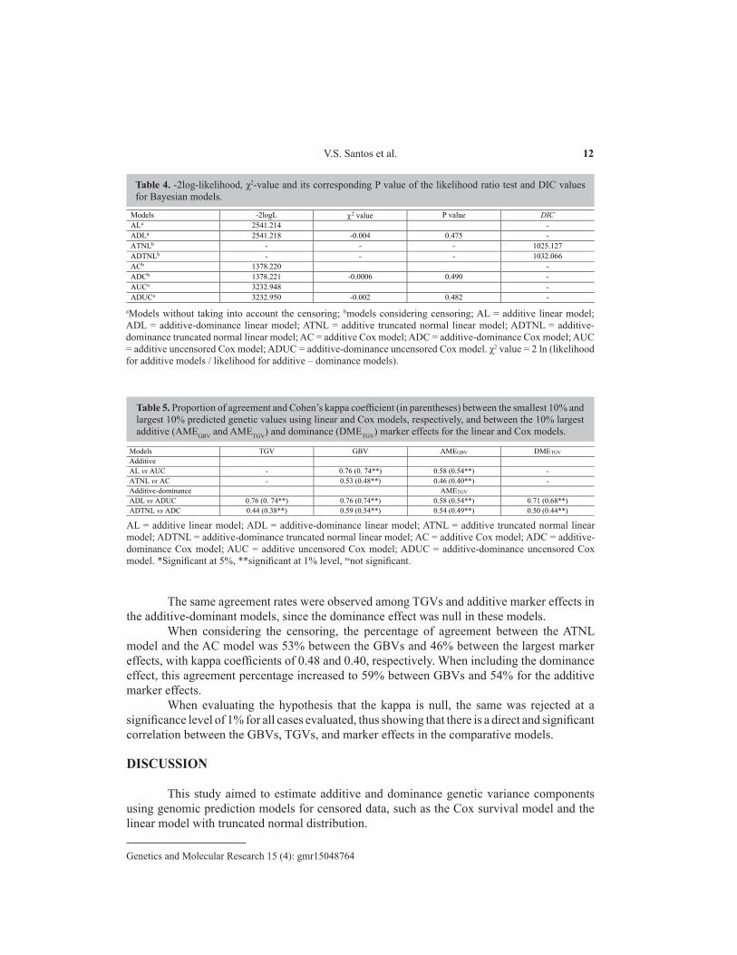
The LRT for models fitted via ML and DIC values for the models fitted via the Bayesian approach are shown in Table 4. According to the LRT, for the three evaluated cases, the hypothesis that the additive model is adequate was not rejected (P value greater than 5%), so we can conclude that the model with additive effects only was the best.

The same occurred for the truncated normal linear model, where the model with additive effects presented with a lower DIC, and was thus more adequate than the model with additive and dominance effects. Ertl et al. (2014), when evaluating the inclusion of dominance effects in dairy cattle, found that LRT was not significant for four of the nine evaluated traits.

The proportion of agreement among the 10% smallest predicted GBVs in the linear model and the 10% largest predicted GBVs in the additive uncensored Cox model was equal to 76% (Table 5), with a kappa equal to 0.74; i.e., of the 34 individuals, 26 were in agreement for both models. For the marker effects, the agreement rate was 58% (14 markers of 24), with a kappa of 0.54.



The same agreement rates were observed among TGVs and additive marker effects in the additive-dominant models, since the dominance effect was null in these models.

When considering the censoring, the percentage of agreement between the ATNL model and the AC model was 53% between the GBVs and 46% between the largest marker effects, with kappa coefficients of 0.48 and 0.40, respectively. When including the dominance effect, this agreement percentage increased to 59% between GBVs and 54% for the additive marker effects.

When evaluating the hypothesis that the kappa is null, the same was rejected at a significance level of 1% for all cases evaluated, thus showing that there is a direct and significant correlation between the GBVs, TGVs, and marker effects in the comparative models.

DISCUSSION

This study aimed to estimate additive and dominance genetic variance components using genomic prediction models for censored data, such as the Cox survival model and the linear model with truncated normal distribution.

aModels without taking into account the censoring; bmodels considering censoring; AL = additive linear model; ADL = additive-dominance linear model; ATNL = additive truncated normal linear model; ADTNL = additive-dominance truncated normal linear model; AC = additive Cox model; ADC = additive-dominance Cox model; AUC = additive uncensored Cox model; ADUC = additive-dominance uncensored Cox model. χ2 value = 2 ln (likelihood for additive models / likelihood for additive – dominance models).

Table 4. -2log-likelihood, χ2-value and its corresponding P value of the likelihood ratio test and DIC values for Bayesian models.

Models -2logL 2 value P value DIC ALa 2541.214 - ADLa 2541.218 -0.004 0.475 - ATNLb - - - 1025.127 ADTNLb - - - 1032.066 ACb 1378.220 - ADCb 1378.221 -0.0006 0.490 - AUCa 3232.948 - ADUCa 3232.950 -0.002 0.482 -

Table 5. Proportion of agreement and Cohen’s kappa coefficient (in parentheses) between the smallest 10% and largest 10% predicted genetic values using linear and Cox models, respectively, and between the 10% largest additive (AMEGBV and AMETGV) and dominance (DMETGV) marker effects for the linear and Cox models.

Models TGV GBV AMEGBV DMETGV Additive AL vs AUC - 0.76 (0. 74**) 0.58 (0.54**) - ATNL vs AC - 0.53 (0.48**) 0.46 (0.40**) - Additive-dominance AMETGV ADL vs ADUC 0.76 (0. 74**) 0.76 (0.74**) 0.58 (0.54**) 0.71 (0.68**) ADTNL vs ADC 0.44 (0.38**) 0.59 (0.54**) 0.54 (0.49**) 0.50 (0.44**)

AL = additive linear model; ADL = additive-dominance linear model; ATNL = additive truncated normal linear model; ADTNL = additive-dominance truncated normal linear model; AC = additive Cox model; ADC = additive-dominance Cox model; AUC = additive uncensored Cox model; ADUC = additive-dominance uncensored Cox model. *Significant at 5%, **significant at 1% level, nsnot significant.



For the linear and Cox models that were fitted by using the lmekin and coxme functions of the coxme package of R, the additive and dominance effects were obtained through Equations 5 and 6, respectively, since in these models only the total genetic effects (sum of additive and non-additive effects) were predicted. This approach is conceptually allowed because it considers the independence between both of the predicted effects (Mrode, 2005).

As reported, the truncated normal linear model fitted via RKHS presented with additive and dominance variance estimates that were much higher than the estimated variances of the linear model fitted via ML. A similar result was observed by Morota et al. (2014) in a study on beef cattle, where they also found that additive and dominance variance estimates were overestimated when using parametric kernels. The authors attributed this to the possible lack of orthogonality between additive (G) and dominance (D) genomic relationship kernels, in that a single kernel captures multiple sources of genetic information.

When including the dominance effect in the truncated normal linear model, the broad sense heritability decreased by approximately 26%. According to Muñoz et al. (2014), this result is expected due to the proportion of dominance variance that can be explained by the additive genetic variance.

In the AUC and ADUC models, the residual variance was equal to 1, in that the random error in latent scale had a standard normal distribution with the probit link function. By accounting for censoring, Yazdi et al. (2002) showed that the error variance can be estimated by the expression 1 / (1 - c) in the Cox model, where c represents the proportion of censored data. In this study, c was equal to 0.56. A summary of the estimations used for heritability in the survival analysis was presented by Resende et al. (2014), who showed that the expression that was used here and was proposed by Yazdi et al. (2002) is the best estimator, as it is valid for the Cox and Weibull models.

There are few studies that include dominance effects in the usual analysis as well as in genomic selection. Moreover, no reports were found in the literature that considered the estimation of the two variance components (additive and dominance) when using survival models. The Survival Kit software (Ducrocq et al., 2010) permits the estimation of only one component at a time and also only allows for the use of the pedigree-based relationship matrix, which makes it impossible to predict genetic values using the genomic relationship matrix. Therefore, comparing both approaches (classical and Bayesian) while using the genomic relationship matrix in the Cox model is not yet possible.

In genomic selection, the correlation between the predicted genomic values and the corrected phenotypes is called of the predictive ability, which is used to assess the quality of fit of the models in the estimation population (Resende et al., 2014). When including the dominance effect, the predictive abilities of the GBVs in the evaluated models did not increase. Similar results were obtained by Ertl et al. (2014) in dairy cattle. According to Nishio and Satoh (2014), this was due to the low and null dominance effects that were obtained in the evaluated models. de Almeida Filho et al. (2016) obtained the highest accuracies in additive-dominant models in relation to additive models only with regards to simulated traits with great dominance effects.

According to Muñoz et al. (2014), additive effects can capture a large proportion of the genetic variance of non-additive effects, such as dominance, due to a possible lack of independence between these effects in improved populations.

The predictive ability values were lowest (around 0.20) in the models where censoring was taken into account (ATNL, ADTNL, AC, and ADC) versus in the models where it was



not considered (LA, LAD, AUC, and ADUC). This occurred because of the greater distance between the predicted genetic values and the adjusted phenotypes of the censored times. Although they presented with the smallest predictive abilities, these models are conceptually more appropriate, since they express the correlations with the phenotypes in the latent scale (Santos et al., 2015).

The uncensored Cox models (AUC and ADUC) presented with the highest Spearman correlations in the AL and ADL models in comparison to the ATNL, ADTNL, AC, and ADC models. This reveals the influence of censoring, since in the AUC and ADUC models, all data were uncensored.

Negative correlations between the linear and Cox models are to be expected, since the random effects in both models are inversely proportional. In the linear model, the fit is performed directly on the time variable, while in the Cox model, the fit is based on the hazard of the animal with regards to obtaining the desired weight at slaughter; i.e., the best animals in the linear models were those with the lowest predicted TGVs and GBVs, since they reached the desired slaughter weight in a shorter period of time. In the Cox models, the best animals were those with the greatest predicted TGVs and GBVs; thus, the risk function grows rapidly, thereby indicating that the animal’s weight also grows quickly (Hou et al., 2009; Giolo and Demétrio, 2011; Santos et al., 2015).

The agreement percentages between predicted genomic values and marker effects were lowest in the models where censoring was considered. In addition to censoring, another factor that played a role in the occurrence was the difference in model fits. The ATNL and ADTNL models were fitted via the Bayesian approach using RKHS, while the AC and ADC models were fitted by the ML method.

In addition, as has been reported, the estimates that were obtained in the ADTNL model were biased because of a lack of orthogonality among additive and dominance genomic relationship kernels (Morota et al., 2014).

In addition to the predictive ability, Cohen’s kappa coefficient has also been employed for evaluating genomic models, as can be seen in Ornella et al. (2014).

Contrary to what has been reported by Onteru et al. (2011), where the implementation of survival models in GS is not yet possible, this study showed that for the method where the pedigree-based relationship matrix is replaced by a marker-based relationship matrix (GBLUP and GBLUP-D in linear models), fitting the Cox model can be conducted relatively simply, without the need for a large computational demand. Furthermore, the fit has allowed for the estimation of non-additive effects, such as the dominance effect.

In addition to the Cox model, other models such as the linear model with truncated normal distribution have been proposed for censored data in GS (Pérez and de los Campos, 2014), thereby expanding the analytical possibilities in additive and non-additive models. However, as mentioned above, the approach that was used for the truncated normal linear model while using the RKHS method overestimated the additive and dominance genetic variance estimates, thus indicating the need for further investigation of this method.

CONCLUSION

This paper showed for the first time and through real data analyses the possibility of performing genomic prediction of censored phenotypes using the Cox survival model with additive and dominance effects. In general, for the assessed trait in the study population, the



dominance variance was null, but on occasion the augmentation of predictive abilities did not include the dominance effect in the assessed models.

Conflicts of interest

The authors declare no conflict of interest.

ACKNOWLEDGMENTS

The first author would like to thank the CAPES (Coordenação de Aperfeiçoamento de Pessoal de Nível Superior) for a Sandwich Doctorate scholarship (grant #BEX 9415/14-9). Research supported by CNPq (Conselho Nacional de Desenvolvimento Científico e Tecnológico) and FAPEMIG (Fundação de Amparo à Pesquisa do Estado de Minas Gerais).

REFERENCES

Azevedo CF, de Resende MD, E Silva FF, Viana JMS, et al. (2015). Ridge, Lasso and Bayesian additive-dominance genomic models. BMC Genet. 16: 105-117. http://dx.doi.org/10.1186/s12863-015-0264-2

Band GO, Guimarães SEF, Lopes PS, Peixoto JDO, et al. (2005). Relationship between the Porcine Stress Syndrome gene and carcass and performance traits in F2 pigs resulting from divergent crosses. Genet. Mol. Biol. 28: 92-96. http://dx.doi.org/10.1590/S1415-47572005000100016

Costa EV, Diniz DB, Veroneze R, Resende MD, et al. (2015). Estimating additive and dominance variances for complex traits in pigs combining genomic and pedigree information. Genet. Mol. Res. 14: 6303-6311. http://dx.doi.org/10.4238/2015.June.11.4

Cox DR (1972). Regression models and life tables (with discussion). J. R. Stat. Soc. Series B Stat. Methodol. 34: 187-220.de Los Campos G, Gianola D and Rosa GJM (2009). Reproducing kernel Hilbert spaces regression: a general framework

for genetic evaluation. J. Anim. Sci. 87: 1883-1887. http://dx.doi.org/10.2527/jas.2008-1259Ducrocq V, Sölkner J and Mészáros G (2010). Survival Kit v6-a Software Package for Survival Analysis (ID232).

Proceedings of the 9th World Congress of Genetic and Applied Livestock Production, Leipzig, 232.Ertl J, Legarra A, Vitezica ZG, Varona L, et al. (2014). Genomic analysis of dominance effects on milk production and

conformation traits in Fleckvieh cattle. Genet. Sel. Evol. 46: 40. http://dx.doi.org/10.1186/1297-9686-46-40de Almeida Filho JE, Guimarães JFR, E Silva FF, de Resende MD, et al. (2016). The contribution of dominance to

phenotype prediction in a pine breeding and simulated population. Heredity (Edinb) 117: 33-41. http://dx.doi.org/10.1038/hdy.2016.23

Giolo SR and Demétrio CGB (2011). A frailty modeling approach for parental effects in animal breeding. J. Appl. Stat. 38: 619-629. http://dx.doi.org/10.1080/02664760903521492

Guo SF, Gianola D, Rekaya R and Short T (2001). Bayesian analysis of lifetime performance and prolificacy in Landrace sows using a linear mixed model with censoring. Livest. Prod. Sci. 72: 243-252. http://dx.doi.org/10.1016/S0301-6226(01)00219-6

Hollander CA, Knol EF, Heuven HCM and van Grevenhof EM (2015). Interval from last insemination to culling: II. Culling reasons from practise and the correlation with longevity. Livest. Sci. 181: 25-30. http://dx.doi.org/10.1016/j.livsci.2015.09.018

Hou Y, Madsen P, Labouriau R, Zhang Y, et al. (2009). Genetic analysis of days from calving to first insemination and days open in Danish Holsteins using different models and censoring scenarios. J. Dairy Sci. 92: 1229-39.

Kärkkäinen HP and Sillanpaa MJ (2013). Fast genomic predictions via Bayesian G-BLUP and multilocus models of threshold traits including censored Gaussian data. G3 (Bethesda) 3: 1511-1523.

Mészáros G, Pálos J, Ducrocq V and Sölkner J (2010). Heritability of longevity in Large White and Landrace sows using continuous time and grouped data models. Genet. Sel. Evol. 42: 13. http://dx.doi.org/10.1186/1297-9686-42-13

Morota G, Boddhireddy P, Vukasinovic N, Gianola D, et al. (2014). Kernel-based variance component estimation and whole-genome prediction of pre-corrected phenotypes and progeny tests for dairy cow health traits. Front. Genet. 5: 56. http://dx.doi.org/10.3389/fgene.2014.00056

Mrode RA (2005). Linear models for the prediction of animal breeding values. CAB International, Wallingford.



Muñoz PR, Resende MF, Jr., Gezan SA, Resende MDV, et al. (2014). Unraveling additive from nonadditive effects using genomic relationship matrices. Genetics 198: 1759-1768. http://dx.doi.org/10.1534/genetics.114.171322

Nishio M and Satoh M (2014). Including dominance effects in the genomic BLUP method for genomic evaluation. PLoS One 9: e85792. http://dx.doi.org/10.1371/journal.pone.0085792

Onteru SK, Fan B, Nikkilä MT, Garrick DJ, et al. (2011). Whole-genome association analyses for lifetime reproductive traits in the pig. J. Anim. Sci. 89: 988-995. http://dx.doi.org/10.2527/jas.2010-3236

Ornella L, Pérez P, Tapia E, González-Camacho JM, et al. (2014). Genomic-enabled prediction with classification algorithms. Heredity (Edinb) 112: 616-626. http://dx.doi.org/10.1038/hdy.2013.144

Pankratz VS, de Andrade M and Therneau TM (2005). Random-effects Cox proportional hazards model: general variance components methods for time-to-event data. Genet. Epidemiol. 28: 97-109. http://dx.doi.org/10.1002/gepi.20043

Pérez P and de los Campos G (2014). Genome-wide regression and prediction with the BGLR statistical package. Genetics 198: 483-495. http://dx.doi.org/10.1534/genetics.114.164442

Pinheiro JC and Bates DM (2000). Mixed-Effects Models in S and S-PLUS. Springer-Verlag, New York.R Development Core Team (2016). R: A Language and Environment for Statistical Computing. Available at http://

www.R-project.org. Accessed March 16, 2016.Resende MDV, Silva FF and Azevedo CF (2014). Estatística matemática, biométrica e computacional: modelos mistos,

multivariados, categóricos e generalizados (REML/BLUP), Inferência Bayesiana, Regressão Aleatória, Seleção Genômica, QTL-GWAS, Estatística Espacial e Temporal, Competição, Sobrevivência. Editora Suprema, Viçosa.

Santos VS, Martins Filho S, Resende MDV, Azevedo CF, et al. (2015). Genomic selection for slaughter age in pigs using the Cox frailty model. Genet. Mol. Res. 14: 12616-12627. http://dx.doi.org/10.4238/2015.October.19.5

Schaeffer L (2013). Survival. In: History of genetic evaluation methods in dairy cattle (Grosu H, Schaeffer L, Oltenacu PA, et al., eds.) 279-298. Available at [https://xa.yimg.com/kq/groups/18395782/1926111600/name/FINAL_BOOK_29.04.2013.pdf]. Accessed 12 April, 2016

Schneider MdelP, Strandberg E, Ducrocq V and Roth A (2005). Survival analysis applied to genetic evaluation for female fertility in dairy cattle. J. Dairy Sci. 88: 2253-2259. http://dx.doi.org/10.3168/jds.S0022-0302(05)72901-5

Serenius T, Stalder KJ and Puonti M (2006). Impact of dominance effects on sow longevity. J. Anim. Breed. Genet. 123: 355-361. http://dx.doi.org/10.1111/j.1439-0388.2006.00614.x

Silva FF, de Resende MD, Rocha GS, Duarte DA, et al. (2013). Genomic growth curves of an outbred pig population. Genet. Mol. Biol. 36: 520-527. http://dx.doi.org/10.1590/S1415-47572013005000042

Smith BJ (2007). boa: An R Package for MCMC Output Convergence Assessment and Posterior Inference. J. Stat. Softw. 21: 1-37. http://dx.doi.org/10.18637/jss.v021.i11

Sobczyńska M and Blicharski T (2015). Phenotypic and genetic variation in longevity of Polish Landrace sows. J. Anim. Breed. Genet. 132: 318-327. http://dx.doi.org/10.1111/jbg.12135

Sorensen DA, Gianola D and Korsgaard IR (1998). Bayesian mixed‐effects model analysis of a censored normal distribution with animal breeding applications. Acta Agric. Scand. Anim. Sci. 48: 222-229.

Su G, Christensen OF, Ostersen T, Henryon M, et al. (2012). Estimating additive and non-additive genetic variances and predicting genetic merits using genome-wide dense single nucleotide polymorphism markers. PLoS One 7: e45293. http://dx.doi.org/10.1371/journal.pone.0045293

Therneau T (2012). Mixed effects Cox models. R package version 2.2-3. http://cran.r-project.org/web/packages/coxme/vignettes/coxme.pdf. Accessed April 12, 2016.

VanRaden PM (2008). Efficient methods to compute genomic predictions. J. Dairy Sci. 91: 4414-4423. http://dx.doi.org/10.3168/jds.2007-0980

Verardo LL, Silva FF, Varona L, Resende MDV, et al. (2015). Bayesian GWAS and network analysis revealed new candidate genes for number of teats in pigs. J. Appl. Genet. 56: 123-132. http://dx.doi.org/10.1007/s13353-014-0240-y

Wang C and Da Y (2014). Quantitative genetics model as the unifying model for defining genomic relationship and inbreeding coefficient. PLoS One 9: e114484. http://dx.doi.org/10.1371/journal.pone.0114484

Yazdi MH, Visscher PM, Ducrocq V and Thompson R (2002). Heritability, reliability of genetic evaluations and response to selection in proportional hazard models. J. Dairy Sci. 85: 1563-1577. http://dx.doi.org/10.3168/jds.S0022-0302(02)74226-4

Genomic prediction for additive and dominance effects of ... · proposed was the GBLUP-D, which...

Documents

Transcript of Genomic prediction for additive and dominance effects of ... · proposed was the GBLUP-D, which...