1

Genomic-enabled prediction based on molecular markers and

pedigree

using the BLR package in R

Paulino Pérez**, Gustavo de los Campos*,**, José Crossa, and Daniel Gianola

P. Pérez, International Maize and Wheat Improvement Center (CIMMYT), Apdo. Postal

6-641, México D.F., México, and Colegio de Postgraduados, Km. 36.5 Carretera

México, Texcoco, Montecillo, Estado de México, 56230, México; G. De los Campos,

University of Wisconsin-Madison, 1675 Observatory Dr. WI 53706, US (present address

University of Alabama at Birmingham, 1665 University Boulevard, Ryals Public Health

Building 414, Birmingham, AL 35294 US); J. Crossa, International Maize and Wheat

Improvement Center (CIMMYT), Apdo. Postal 6-641, México D.F., México; D. Gianola,

University of Wisconsin-Madison, 1675 Observatory Dr. WI 53706, US. *Corresponding

author (gcampos@ms.soph.uab.edu ). ** The first two authors made an equal contribution.

Abbreviations: GS, Genomic selection; BLR, Bayesian Linear Regression; RR, ridge

regression; BRR, Bayesian Ridge Regression; BL, Bayesian LASSO; BLUP, Best

Linear Unbiased Prediction.

2

Abstract

The availability of molecular markers has made possible the use of genomic

selection in plant and animal breeding. However, models for genomic selection pose

several computational and statistical challenges and require specialized computer

programs not always available to the end user and not implemented in standard

statistical software yet. The R BLR (Bayesian Linear Regression) package implements

several statistical procedures (i.e., Bayesian Ridge Regression, Bayesian Lasso) in a

unified framework that allows including marker genotypes and pedigree data jointly.

This article describes the classes of models implemented in the BLR package and

illustrates their use through examples using simulated and real data from plant breeding

trials. Also addressed are some challenges faced when applying genomic-enabled

selection, such as model choice, evaluation of predictive ability through cross-validation,

and choice of hyper-parameters.

Introduction

Prediction of genetic values is a central problem in quantitative genetics. Over many

decades such predictions have been obtained using phenotypic and family data, the latter usually

represented by a pedigree. Accurate predictions of genetic values of genotypes whose

phenotypes are yet to be observed (e.g., newly developed lines) are needed to attain rapid genetic

progress and reduce phenotyping costs (e.g., Bernardo and Yu, 2007). However, pedigree-based

models typically do not account for Mendelian segregation, a term that in an additive model and

in the absence of inbreeding explains as much as one half of the genetic variance. This sets an

3

upper limit on the accuracy of estimates of genetic values of individuals without progeny. Dense

molecular markers (MM) are now available in the genome of humans and of many plant and

animal species. Unlike pedigree data, MM allow tracing back Mendelian segregation events at

many points along the genome. Potentially, this information can be used to improve the accuracy

of estimates of genetic values of newly developed lines.

Following the ground-breaking contribution of Meuwissen et al. (2001), genomic

selection (GS) has gained ground in plant and animal breeding (e.g., Bernardo and Yu, 2007;

Hayes et al., 2009; VanRaden et al., 2009; de los Campos et al., 2009; Crossa et al., 2010). In

practice, implementing GS involves analyzing large amounts of phenotypic and MM data, and

requires specialized computer programs. The main purpose of this article is to show how the R

(R Development Core Team, 2009) BLR (Bayesian Linear Regression) package can be used to

implement several models for GS. A first version of the algorithms and the R-code implemented

in the package was presented in de los Campos et al. (2009). The package was developed further

and its performance was significantly improved by the first two authors of this article; it is now

freely available through the R website. We provide a brief overview of parametric models for GS

and describe the type of models implemented in BLR. We show two applications that illustrate

the use of the package and several features of the models implemented in it. The package and

data set are available from the R website, http://www.r-project.org.

4

Parametric models for genomic selection

In parametric models for GS (e.g., Meuwissen et al., 2001), phenotypic outcomes, iy

( )ni ,...,1= , are regressed on marker covariates ijx ( )pj ,...,1= using a linear model of the form

ij

p

jiji xy εβ += ∑

=1

, where jβ is the regression of iy on the jth

marker covariate and iε is a model

residual. In matrix notation, the regression model is expressed as εXβy += , where { }iy=y ,

{ }ijx=X , { }jβ=β and { }iε=ε . The number of molecular markers (p) is usually larger than the

number of observations (n) and, because of this, estimation of marker effects via multiple

regression by ordinary least squares (OLS) is not feasible. Instead, penalized estimation methods

such as ridge regression (RR, Hoerl and Kennard, 1970), or LASSO, or Bayesian methods such

as those of Meuwissen et al. (2001) or the Bayesian LASSO (BL) of Park and Casella (BL,

2008) (e.g., Yi and Xu, 2008; de los Campos et al., 2009) can be used to estimate marker effects.

In RR, estimates of the effects of MM are obtained as the solution to the following

optimization problem: ( )

+−= ∑∑==

p

jj

n

iiiy

1

2

1

2 ~'minargˆ βλβxβ

β

. Here, 0~≥λ is a regularization

parameter controlling the trade-offs between goodness of fit, as measured by the residual sum of

squares, and model complexity, with the latter measured by the sum of squared marker effects,

∑=

p

j

j

1

2β . The first order conditions of the above optimization problem are satisfied by

[ ] yXβIXX ′=+′ ˆ~λ ; equivalently, [ ] yXIXXβ ′+′=

−1~ˆ λ . Relative to OLS, RR adds a constant,λ~

,

to the diagonal of the matrix of coefficients; this makes the solution unique and shrinks estimates

5

of marker effects towards zero, with the extent of shrinkage increasing as λ~

increases (with

0~=λ the solution to the above problem is the OLS estimate of marker effects).

From a Bayesian perspective, β̂ can be viewed as the conditional posterior mode in a

model with Gaussian likelihood and IID (independent and identically distributed) Gaussian

marker effects, that is,

( )

( ) ( )

=

=

∏

∏ ∑

=

= =

,0 :Prior

,, :Likelihood

1

22

1

2

1

2

n

ij

n

i

p

jjiji

Np

xyNp

ββ

εε

σβσ

σβσ

β

βy

[1]

Above, 2βσ is the variance of marker effects, a priori. The prior distribution of marker effects

becomes increasingly informative and concentrated around zero as 2βσ decreases. The posterior

mean and mode of β from [1] is equal to the ridge-regression estimate, with 22~εβ σσλ −= , that is,

( ) [ ] yXIXXβyβ ′+′==−− 122ˆ

εβ σσE . Therefore, prediction of genetic values from [1] can be

obtained as

( ) ( )[ ] yXIXXX

yβXyXβ

′+′=

=−− 122

2222

,,,,

βε

βεβε

σσ

σσσσ EE [2a]

Alternatively, from [1] and using properties of the multivariate normal distribution, one has:

( ) ( ) ( )

[ ][ ] yIXXXX

yIXXXX

yyyXβyXβ

122

1222

122

,,,

−−

−

−

+′′=

+′′=

′=

βε

εββ

βε

σσ

σσσ

σσ VarCovE

[2b]

6

Formulae [2a] and [2b] are equivalent and correspond the Best Linear Unbiased Predictor

(BLUP) under the model defined by [1]. Note that [2a] and [2b] require solving systems of p and

n equations, respectively. Therefore, with p>>n expression [2b] is computationally more

convenient. However, unlike [2a], expression [2b] does not yield estimates of marker effects.

In RR-BLUP, estimates of marker effects are penalized to the same extent, and this may

not be appropriate if some markers are located in regions not associated with genetic variance

whereas others are linked to QTLs (Goddard and Hayes, 2007). To overcome this limitation,

methods performing variable selection and shrinkage (e.g., the Least Absolute Value Selection

and Shrinkage Operator, LASSO, Tibshirani, 1996) or Bayesian methods using marker-specific

shrinkage of effects, such as methods BayesA of Meuwissen et al. (2001) or the BL of Park and

Casella (2008), have been proposed.

The BLR package implements Bayesian regression with marker-specific (BL) or marker

homogenous (Bayesian RR) shrinkage of estimates effects. The package allows inclusion of

covariates other than markers, and regressions on a pedigree as well. In BLR, phenotypes are

expressed as follows:

εβXβXZuβX1y +++++= LLRRFFµ [3]

where y , the response, is an (n×1) vector (missing values are allowed); µ is an intercept;

{ }FpnFijF x

×=X , { }

Upnijz ×=Z , { }

RpnRijR x×

=X and { }LpnRijL x

×=X are incidence matrices for

the vectors of effects Fβ , u, Rβ and Lβ , whose dimensions are LRUF pppp and ,, , respectively.

These vectors of effects differ with respect to the prior distributions assigned, as discussed later

7

on. Finally, ε is a vector of model residuals assumed to be distributed as

2

2

~iw

DiagN εσ0,ε ,

where 2

εσ is an (unknown) variance parameter and the iw ’s are (known) weights that allow for

heterogeneous-residual variances. From these assumptions, the conditional distribution of the

data, given the location effects, the residual variance and the weights, is:

( ) ∏ ∑∑∑∑= ====

++++=

n

i i

p

j

KjLij

p

j

RjRij

p

j

jij

p

j

FjFijiLRFw

xxuzxyNpLRUF

12

1111

,,,,, εσβββµµ ββuβy [4]

Any of the elements on the right-hand side of [3], except µ and ε , can be excluded in BLR; by

default, the program runs an intercept model, i.e., iiy εµ += . If weights are not provided, all

weights are set equal to one.

The Bayesian model is completed by assigning a prior to the collection of model

unknowns, { }2222 ,,,,,,,,, εβ σλσσµ τββuβθ LRuF R= . The intercept, µ , and the vector of ‘fixed’

effects, Fβ , are assigned flat priors, that is, ( ) tconsp F tan, ∝βµ . This treatment yields

posterior means of these unknowns that are similar to those obtained with OLS, provided only µ

and βF are fitted.

The vector u is modeled using the standard assumptions of the infinitesimal additive

model (e.g., Fisher, 1918; Wright, 1921; Henderson, 1975), that is, ( ) ( )22uu Np σσ A0,u = , where

A is a positive-definite matrix (usually a numerator relationship matrix computed from a

pedigree) and 2

uσ is an unknown variance, whose prior is an Inverse-Chi square density with

degrees of freedom udf and scale uS , that is, ( )uuuu Sdf ,222 ~ σχσ − ; the hyper-parameters are user

8

provided In the parameterization used in BLR, 12 )2()|( −−= uuuuu dfSSdfE ,σ . The multivariate

normal prior assigned to u induces shrinkage of estimates of effects uj, towards zero to an extent

depending on the ratio 22 −εσσ u and on the amount of inbreeding, as well as borrowing of

information between pairs of levels of the random effect, { }jj uu ′, , depending on the

relationships between individuals in the pedigree.

The vector of regression coefficients Rβ is assigned a Gaussian prior with variance

common to all effects, that is, ( ) ( )∏=

=R

RR

p

jRjR Np

1

22 ,0 ββ σβσβ . This prior induces estimates that

are the Bayesian counterpart of those obtained with Ridge Regression; we refer to this as

‘Bayesian Ridge Regression’ (BRR). The variance parameter, 2

Rβσ , is treated as unknown and is

assigned a scaled inverse- 2χ prior density, that is, ( ) ( )RRRR

Sdfp ββββ σχσ ,222 −= with degrees of

freedom, R

df β , and scale, R

Sβ , provided by the user.

The vector of regression coefficients Lβ is treated as in the Bayesian LASSO of Park and

Casella (2008); the conditional prior distribution of marker effects, ( )22 , εστβ Lp , is Gaussian

with marker-specific prior variances, that is, ( ) ( )∏=

=Lp

jjLjL Np

1

2222 ,0, τσβσ εετβ . Unlike BRR, this

induces marker-specific shrinkage of estimates of effects, whose extent depends on 2−jτ . The

variance parameters, 2jτ , are assigned exponential IID priors, ( ) ( )∏

=

=Lp

jjExpp

1

222 λτλτ . Finally,

in the BLR package, the prior distribution of the regularization parameterλ , ( )λp , can be:

(a) a mass-point at some value (i.e., fixed λ ),

9

(b) ( ) ( )δλ ,~2 rGammap t as suggested by Park and Casella (2008), or

(c) ( )

∝ 2121 ,

max,max, αα

λααλ Betap (de los Campos et al., 2009).

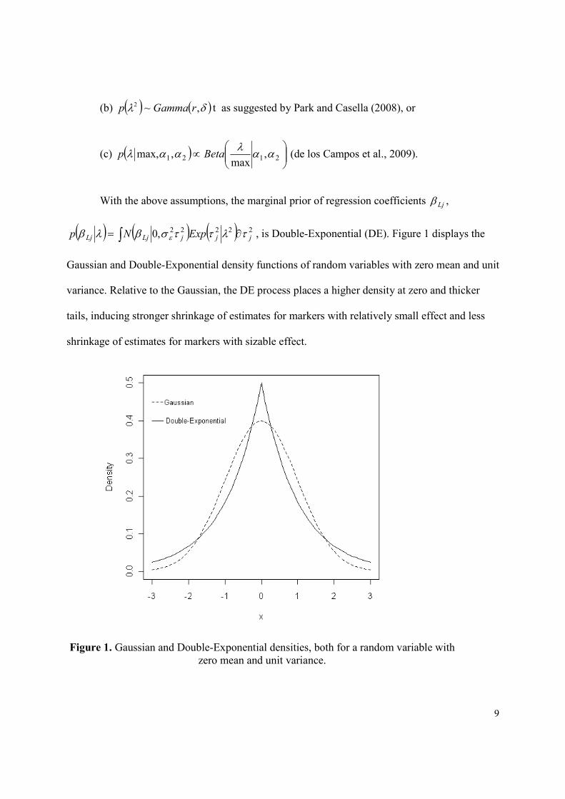
With the above assumptions, the marginal prior of regression coefficients Ljβ ,

( ) ( ) ( )∫ ∂= 22222,0 jjjLjLj ExpNp τλττσβλβ ε , is Double-Exponential (DE). Figure 1 displays the

Gaussian and Double-Exponential density functions of random variables with zero mean and unit

variance. Relative to the Gaussian, the DE process places a higher density at zero and thicker

tails, inducing stronger shrinkage of estimates for markers with relatively small effect and less

shrinkage of estimates for markers with sizable effect.

Figure 1. Gaussian and Double-Exponential densities, both for a random variable with

zero mean and unit variance.

10

Finally, the residual variance is assigned a scaled inverse- 2χ prior density with degrees

of freedom, εdf , and scale parameter provided by the user, εS , that is,

( )

= −

εεεε σχσ Sdfp ,222 .

Collecting the aforementioned assumptions, the prior distribution in BLR is:

( ) ( ) ( ) ( )

( ) ( ) ( ) ( ).,0

,0

22

1

22

1

22

1

2222

εεεε

ββββ

σχλλττσβ

σχσβσ

SdfpExpN

SdfNNp

LL

R

RRRR

p

jj

p

jjLj

p

jRju

,

,A0,uθ

−

==

=

−

×

∝

∏∏

∏

The prior distribution is indexed by several hyper-parameters; in the Appendix we

provide guidelines for choosing these parameters based on prior expectations about the

proportion of phenotypic variance that can be attributed to each of the components on the right-

hand side of [3].

The posterior distribution of model unknowns is proportional to the product of the

likelihood and the prior distribution, that is:

( )

( )( ) ( )

( ) ( ) ( )

( )εεε

ε

ββββ

ε

σχ

λλττσβ

σχσβ

σ

σβββµ

Sdf

pExpN

SdfN

N

wxxuzxyNp

LL

R

RRRR

LRUF

p

jj

p

jjLj

p

jRj

u

n

i i

p

jKjLij

p

jRjRij

p

jjij

p

jFjFiji

,

,

A0,u

yθ

22

1

22

1

22

1

222

2

12

1111

,0

,0

,

−

==

=

−

= ====

×

×

×

×

++++∝

∏∏

∏

∏ ∑∑∑∑

[5]

11

This posterior distribution does not have a closed form; however, a Gibbs sampler can be

used to draw samples from it. The Gibbs sampler is as in de los Campos et al. (2009), but

extended to accommodate “fixed” effects and BRR.

Using BLR

This section gives two examples that illustrate the use of the BLR package and describe

features of the models. It is assumed that the reader is familiar with the R-language/environment.

In Example 1, we study the impact of different shrinkage methods (BRR vs BL) using simulated

data. Example 2 illustrates how the package can be used to implement cross-validation (CV)

using Bayesian methods. Cross-validation can be used for model comparison (e.g., to compare

predictive ability of pedigree-based models versus marker-based models) or for selecting model

parameters of the model (e.g., λ in the BL). Both examples make use of a wheat data set made

available with the package, whose main features are described next.

Wheat data set

This data , used by Crossa et al. (2010), contains a historical set of 599 wheat lines from

CIMMYT’s Global Wheat Program that were genotyped for 1447 Diversity Array Technology

markers (DArT, Triticarte Pty. Ltd, Canberra, Australia; http://www.triticarte.com.au) and

evaluated for grain yield (GY) in four macro-environments. The dataset becomes available in the

R environment by running the following R-code:

library(BLR) data(wheat)

12

Function library()loads the package, and data() loads datasets included in the package

into the environment. The above code also loads the following objects (type objects() in the R

console to list them) into the environment:

- Y, a matrix (599×4) containing the 2-year average grain yield of each of these lines in

each of the four environments (phenotypes were standardized to a sample variance equal

to one in each of the environments);

- A (599×599) is a numerator relationship matrix computed from a pedigree that traced

back many generations. This relationship matrix was derived using the Browse

application of the International Crop Information System (ICIS), as described in

http://cropwiki.irri.org/icis/index.php/TDM_GMS_Browse (McLaren, 2005);

- X (599×1279) is a matrix with DArT genotypes; data are from pure lines and genotypes

were coded as 0/1 denoting the absence/presence of the DArT. Markers with a minor

allele frequency lower than 0.05 were removed, and missing genotypes were imputed

with samples from the marginal distribution of marker genotypes, that is, ijx = Bernoulli(

jp̂ ), where jp̂ is the estimated allele frequency computed from the non-missing

genotypes. The number of DArT MMs after edition was 1279.

- sets (599×1) is a vector that assigns observations to 10 disjoint sets; the assignment was

generated at random. This is used later to conduct a 10-fold CV.

Pedigree information was included in addition to marker data.

13

Example 1: The nature of different shrinkage methods

As stated, BRR or BL use different priors for marker effects; this induces different types

of shrinkage of estimates of such effects. The simulation presented in this section aims at

illustrating these differences. Data were generated using marker genotypes from the wheat

dataset (X) with marker effects and model residuals simulated as described below.

Data simulation

Data were simulated under an additive model of the form,

,599,...,1,1279

1

=++= ∑=

ixy ij

j

jiji εβµ

where 100=µ is an effect common to all individuals; { }ijx

are marker genotypes from a collection of wheat lines described previously;{ }jβ are marker

effects; and ( )1,0N~ ii εε are IID standard normal residuals. We assumed that most markers

(1267) had a relatively small effect and that only a few (12) had a sizable effect. Specifically,

marker effects were sampled from the following mixture model:

( ) { }( ) { }

( )

otherwise. k0,N

1279,1047,815,583,351,119 if 0.5,0.8Uniform

63699,931,113,235,467, if 0.5,-0.8-Uniform

∈

∈

= j

j

jβ

where -11279k = . The R-code used to implement this simulation was:

14

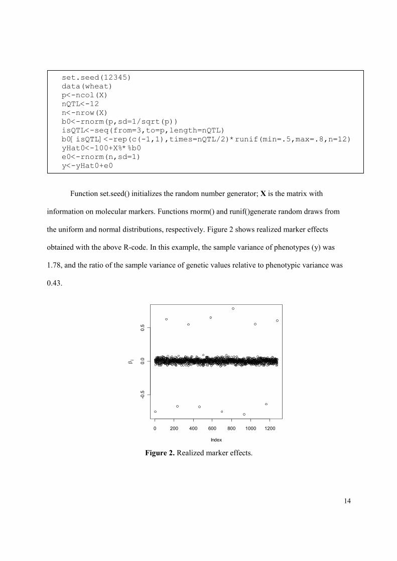
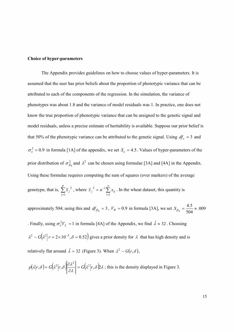
Function set.seed() initializes the random number generator; X is the matrix with

information on molecular markers. Functions rnorm() and runif()generate random draws from

the uniform and normal distributions, respectively. Figure 2 shows realized marker effects

obtained with the above R-code. In this example, the sample variance of phenotypes (y) was

1.78, and the ratio of the sample variance of genetic values relative to phenotypic variance was

0.43.

Figure 2. Realized marker effects.

0 200 400 600 800 1000 1200

-0.5

0.0

0.5

Index

βj

set.seed(12345) data(wheat) p<-ncol(X) nQTL<-12 n<-nrow(X) b0<-rnorm(p,sd=1/sqrt(p)) isQTL<-seq(from=3,to=p,length=nQTL) b0[isQTL]<-rep(c(-1,1),times=nQTL/2)*runif(min=.5,max=.8,n=12) yHat0<-100+X%*%b0 e0<-rnorm(n,sd=1) y<-yHat0+e0

15

Choice of hyper-parameters

The Appendix provides guidelines on how to choose values of hyper-parameters. It is

assumed that the user has prior beliefs about the proportion of phenotypic variance that can be

attributed to each of the components of the regression. In the simulation, the variance of

phenotypes was about 1.8 and the variance of model residuals was 1. In practice, one does not

know the true proportion of phenotypic variance that can be assigned to the genetic signal and

model residuals, unless a precise estimate of heritability is available. Suppose our prior belief is

that 50% of the phenotypic variance can be attributed to the genetic signal. Using 3=εdf and

9.02 =εσ in formula [1A] of the appendix, we set 5.4=εS . Values of hyper-parameters of the

prior distribution of 2

Rβσ and 2λ can be chosen using formulae [3A] and [4A] in the Appendix.

Using these formulae requires computing the sum of squares (over markers) of the average

genotype, that is, ∑=

.

1

2p

jjx , where ∑

=

−=n

iijj xnx

1

12. In the wheat dataset, this quantity is

approximately 504; using this and 3=R

df β , 9.0=RV in formula [3A], we set 009.504

5.4≈=

RSβ

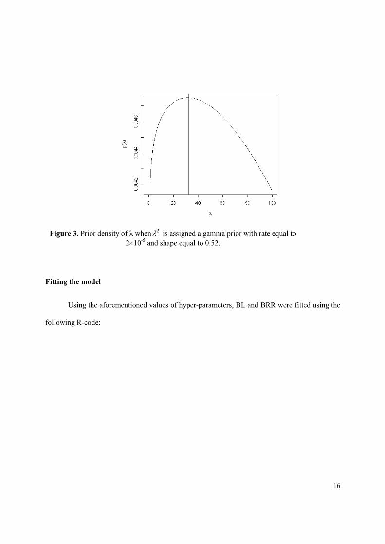
. Finally, using 12 =LVεσ in formula [4A] of the Appendix, we find 32ˆ ≈λ . Choosing

( )52.0,102 ~ 522 =×= − δλλ rG gives a prior density for λ that has high density and is

relatively flat around 32ˆ =λ (Figure 3). When ( )δλ ,~2 rG ,

( ) ( ) ( ) λδλλλ

δλδλ 2,,, 22

2 rGrGrp =∂∂

= ; this is the density displayed in Figure 3.

16

Figure 3. Prior density of λ when 2λ is assigned a gamma prior with rate equal to

2×10-5

and shape equal to 0.52.

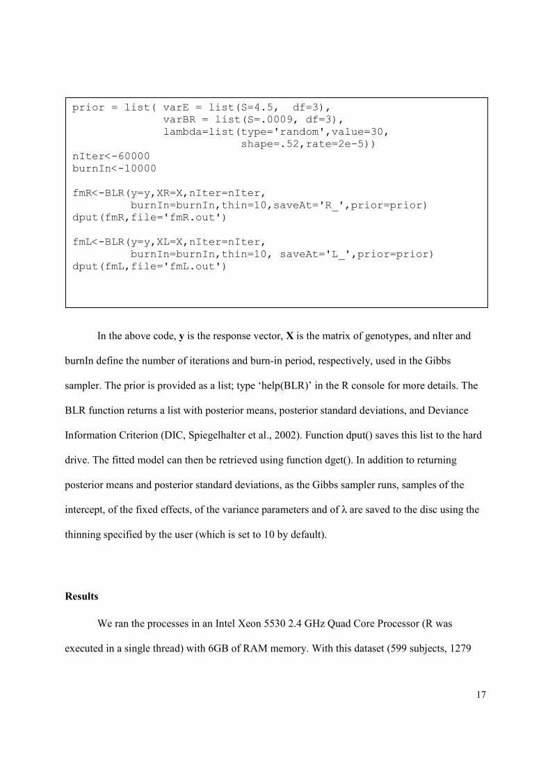
Fitting the model

Using the aforementioned values of hyper-parameters, BL and BRR were fitted using the

following R-code:

17

In the above code, y is the response vector, X is the matrix of genotypes, and nIter and

burnIn define the number of iterations and burn-in period, respectively, used in the Gibbs

sampler. The prior is provided as a list; type ‘help(BLR)’ in the R console for more details. The

BLR function returns a list with posterior means, posterior standard deviations, and Deviance

Information Criterion (DIC, Spiegelhalter et al., 2002). Function dput() saves this list to the hard

drive. The fitted model can then be retrieved using function dget(). In addition to returning

posterior means and posterior standard deviations, as the Gibbs sampler runs, samples of the

intercept, of the fixed effects, of the variance parameters and of λ are saved to the disc using the

thinning specified by the user (which is set to 10 by default).

Results

We ran the processes in an Intel Xeon 5530 2.4 GHz Quad Core Processor (R was

executed in a single thread) with 6GB of RAM memory. With this dataset (599 subjects, 1279

prior = list( varE = list(S=4.5, df=3), varBR = list(S=.0009, df=3), lambda=list(type='random',value=30,

shape=.52,rate=2e-5)) nIter<-60000 burnIn<-10000 fmR<-BLR(y=y,XR=X,nIter=nIter, burnIn=burnIn,thin=10,saveAt='R_',prior=prior) dput(fmR,file='fmR.out') fmL<-BLR(y=y,XL=X,nIter=nIter, burnIn=burnIn,thin=10, saveAt='L_',prior=prior) dput(fmL,file='fmL.out')

18

markers) the process took about 1% of RAM memory. BRR took about 5.5 seconds for every

1000 iterations of the sampler; BL takes about twice as much time.

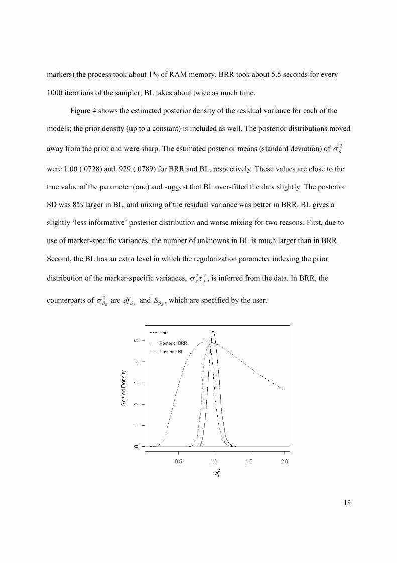
Figure 4 shows the estimated posterior density of the residual variance for each of the

models; the prior density (up to a constant) is included as well. The posterior distributions moved

away from the prior and were sharp. The estimated posterior means (standard deviation) of 2εσ

were 1.00 (.0728) and .929 (.0789) for BRR and BL, respectively. These values are close to the

true value of the parameter (one) and suggest that BL over-fitted the data slightly. The posterior

SD was 8% larger in BL, and mixing of the residual variance was better in BRR. BL gives a

slightly ‘less informative’ posterior distribution and worse mixing for two reasons. First, due to

use of marker-specific variances, the number of unknowns in BL is much larger than in BRR.

Second, the BL has an extra level in which the regularization parameter indexing the prior

distribution of the marker-specific variances, 22

jτσ ε , is inferred from the data. In BRR, the

counterparts of 2

Rβσ are

Rdf β and

RSβ , which are specified by the user.

19

Figure 4. Prior and estimated posterior density of the residual variance, by model

(BRR=Bayesian Ridge Regression; BL=Bayesian LASSO).

The posterior mean of λ in BL was 20.0, and a 95th

highest posterior density confidence

region was bounded by [15.24, 25.2]. These results also indicate that the posterior distribution of

λ moved away from the prior (Figure 3), indicating that Bayesian learning takes place.

Measures of goodness of fit and model complexity (pD=estimated effective number of

parameters, Spiegelhalter et al., 2002, and DIC) are included in the fitted object. This can be

assessed with the following code:

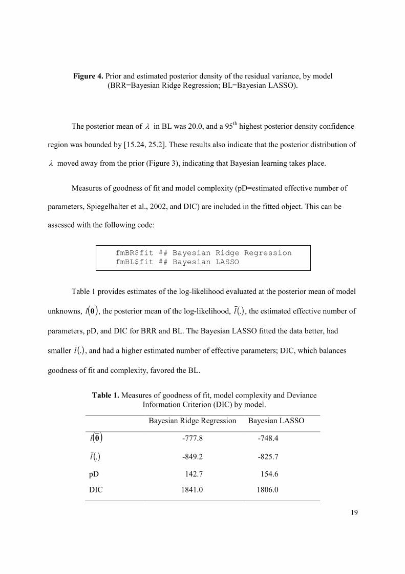
Table 1 provides estimates of the log-likelihood evaluated at the posterior mean of model

unknowns, ( )θl , the posterior mean of the log-likelihood, ( ).l , the estimated effective number of

parameters, pD, and DIC for BRR and BL. The Bayesian LASSO fitted the data better, had

smaller ( ).l , and had a higher estimated number of effective parameters; DIC, which balances

goodness of fit and complexity, favored the BL.

Table 1. Measures of goodness of fit, model complexity and Deviance

Information Criterion (DIC) by model.

Bayesian Ridge Regression Bayesian LASSO

( )θl -777.8 -748.4

( ).l -849.2 -825.7

pD 142.7 154.6

DIC 1841.0 1806.0

fmBR$fit ## Bayesian Ridge Regression fmBL$fit ## Bayesian LASSO

20

( )θl = log-likelihood evaluated at the estimated posterior mean of model

unknowns; ( ).l =estimated posterior mean of the log-likelihood;

pD=estimated effective number of parameters.

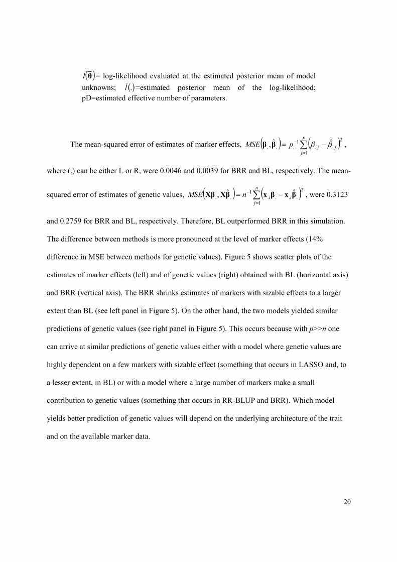
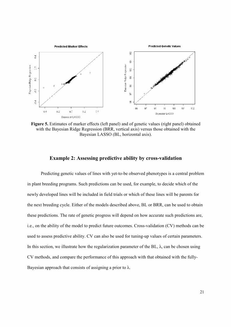
The mean-squared error of estimates of marker effects, ( ) ( )∑=

− −=p

jjjpMSE

1

2

..1

...ˆˆ, ββββ ,

where (.) can be either L or R, were 0.0046 and 0.0039 for BRR and BL, respectively. The mean-

squared error of estimates of genetic values, ( ) ( )∑=

− −=n

jiinMSE

1

2

....1

..ˆˆ, βxβxβXXβ , were 0.3123

and 0.2759 for BRR and BL, respectively. Therefore, BL outperformed BRR in this simulation.

The difference between methods is more pronounced at the level of marker effects (14%

difference in MSE between methods for genetic values). Figure 5 shows scatter plots of the

estimates of marker effects (left) and of genetic values (right) obtained with BL (horizontal axis)

and BRR (vertical axis). The BRR shrinks estimates of markers with sizable effects to a larger

extent than BL (see left panel in Figure 5). On the other hand, the two models yielded similar

predictions of genetic values (see right panel in Figure 5). This occurs because with p>>n one

can arrive at similar predictions of genetic values either with a model where genetic values are

highly dependent on a few markers with sizable effect (something that occurs in LASSO and, to

a lesser extent, in BL) or with a model where a large number of markers make a small

contribution to genetic values (something that occurs in RR-BLUP and BRR). Which model

yields better prediction of genetic values will depend on the underlying architecture of the trait

and on the available marker data.

21

Figure 5. Estimates of marker effects (left panel) and of genetic values (right panel) obtained

with the Bayesian Ridge Regression (BRR, vertical axis) versus those obtained with the

Bayesian LASSO (BL, horizontal axis).

Example 2: Assessing predictive ability by cross-validation

Predicting genetic values of lines with yet-to-be observed phenotypes is a central problem

in plant breeding programs. Such predictions can be used, for example, to decide which of the

newly developed lines will be included in field trials or which of these lines will be parents for

the next breeding cycle. Either of the models described above, BL or BRR, can be used to obtain

these predictions. The rate of genetic progress will depend on how accurate such predictions are,

i.e., on the ability of the model to predict future outcomes. Cross-validation (CV) methods can be

used to assess predictive ability. CV can also be used for tuning-up values of certain parameters.

In this section, we illustrate how the regularization parameter of the BL, λ, can be chosen using

CV methods, and compare the performance of this approach with that obtained with the fully-

Bayesian approach that consists of assigning a prior to λ.

22

Model

The linear model [NOTE: the term “data equation is often used in social scienes but it is

bad. An equation typically involves a system which needs to be solved for unknowns as opposed

to a formulation of how one thinks observations are generated in nature: a model] is

εuβX1y +++= LLµ . We chose values of hyper-parameters using formulae presented in the

Appendix. As in Example 1, it was assumed a priori that 50% of the phenotypic variance (which

equals to one because phenotypes were standardized to a unit variance) could be attributed to

genetic values. With this, and using 3=εdf in formula [1A] in the Appendix, we obtained

5.2=εS . Further, we assumed a priori that one half of the variance of genetic values can be

accounted for by the regression on markers, LLβX , and that the regression on the pedigree, u ,

accounted for the other half. With this, and using 3=udf and 98.1=a in [2A], we obtained

63.0=uS . Finally, using 504.

1

2

1

1 =

∑ ∑= =

−p

j

n

iLijxn in formula [4A] in the Appendix, we obtained

455041

4

2

122ˆ 212 ≈== ∑−

Rp

jLjL xVεσλ . Choosing ( )52.0,101~ 522 =×= − δλλ rG gives a prior

for λ that has a maximum and is relatively flat in the neighborhood of 45.

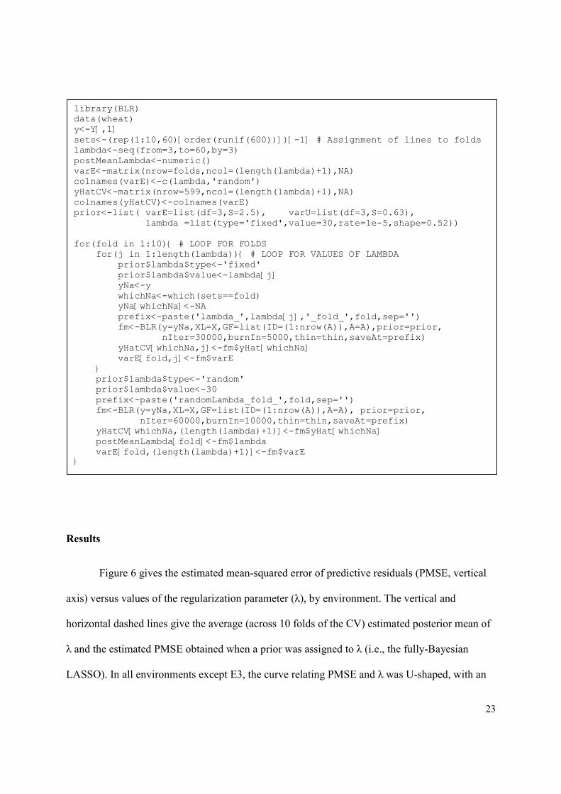
The following R-code illustrates how this CV was carried out for the first trait. The

vector sets assign lines to folds of the CV. The code involves two loops: the outer loop runs over

folds of the CV; the inner loop fits models over a grid of values of λ. For every fold in the outer

loop, the phenotypes of approximately 60 lines are declared as missing values; the fitted model

yields a prediction of the performance of these lines.

23

Results

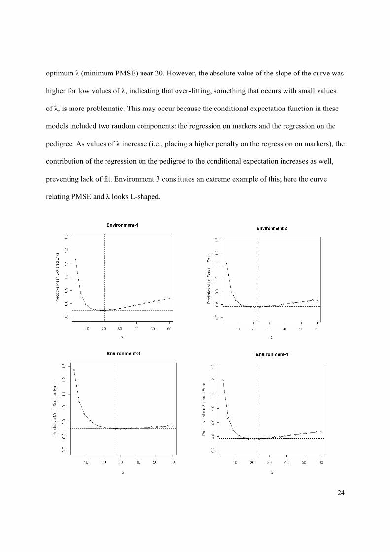
Figure 6 gives the estimated mean-squared error of predictive residuals (PMSE, vertical

axis) versus values of the regularization parameter (λ), by environment. The vertical and

horizontal dashed lines give the average (across 10 folds of the CV) estimated posterior mean of

λ and the estimated PMSE obtained when a prior was assigned to λ (i.e., the fully-Bayesian

LASSO). In all environments except E3, the curve relating PMSE and λ was U-shaped, with an

library(BLR) data(wheat) y<-Y[,1] sets<-(rep(1:10,60)[order(runif(600))])[-1] # Assignment of lines to folds lambda<-seq(from=3,to=60,by=3) postMeanLambda<-numeric() varE<-matrix(nrow=folds,ncol=(length(lambda)+1),NA) colnames(varE)<-c(lambda,'random') yHatCV<-matrix(nrow=599,ncol=(length(lambda)+1),NA) colnames(yHatCV)<-colnames(varE) prior<-list( varE=list(df=3,S=2.5), varU=list(df=3,S=0.63), lambda =list(type='fixed',value=30,rate=1e-5,shape=0.52)) for(fold in 1:10){ # LOOP FOR FOLDS for(j in 1:length(lambda)){ # LOOP FOR VALUES OF LAMBDA prior$lambda$type<-'fixed' prior$lambda$value<-lambda[j] yNa<-y whichNa<-which(sets==fold) yNa[whichNa]<-NA prefix<-paste('lambda_',lambda[j],'_fold_',fold,sep='') fm<-BLR(y=yNa,XL=X,GF=list(ID=(1:nrow(A)),A=A),prior=prior, nIter=30000,burnIn=5000,thin=thin,saveAt=prefix) yHatCV[whichNa,j]<-fm$yHat[whichNa] varE[fold,j]<-fm$varE } prior$lambda$type<-'random' prior$lambda$value<-30 prefix<-paste('randomLambda_fold_',fold,sep='') fm<-BLR(y=yNa,XL=X,GF=list(ID=(1:nrow(A)),A=A), prior=prior, nIter=60000,burnIn=10000,thin=thin,saveAt=prefix) yHatCV[whichNa,(length(lambda)+1)]<-fm$yHat[whichNa] postMeanLambda[fold]<-fm$lambda varE[fold,(length(lambda)+1)]<-fm$varE }

24

optimum λ (minimum PMSE) near 20. However, the absolute value of the slope of the curve was

higher for low values of λ, indicating that over-fitting, something that occurs with small values

of λ, is more problematic. This may occur because the conditional expectation function in these

models included two random components: the regression on markers and the regression on the

pedigree. As values of λ increase (i.e., placing a higher penalty on the regression on markers), the

contribution of the regression on the pedigree to the conditional expectation increases as well,

preventing lack of fit. Environment 3 constitutes an extreme example of this; here the curve

relating PMSE and λ looks L-shaped.

25

Figure 6. Predictive mean squared error (PMS, vertical axis) versus values of the regularization

parameter of the Bayesian LASSO (horizontal axis), by environment. The vertical and horizontal

dashed lines give the average (across 10 folds of the cross-validation) estimated posterior mean

of λ and the estimated PMSE obtained when a prior was assigned to λ.

The posterior modes of λ were always considerably smaller than the prior mode (45),

indicating that Bayesian learning took place. In all environments, the fully-Bayesian treatment

yielded posterior means of λ that were in the neighborhood of the optimal values found when

models were run over a grid of values of this unknown. Also, predictive ability of models with

random λ was as good as the best obtained when CV was used for choosing λ. These results

suggest that,at least for these traits and this population, the fully-Bayesian treatment, which

consists of inferring λ from the data, yields good results.

Concluding remarks

The BLR package allows fitting high-dimensional linear regression models including

dense molecular markers, pedigree information and covariates other than markers. The interface

allows the user to choose models (e.g, BL versus BRR) and prior hyper-parameters easily. The

algorithms implemented are relatively efficient and models with a modest number of markers

(e.g., ~1000) can be fitted in a standard PC easily. The routines implemented in the package have

also been used successfully in problems with larger numbers of molecular markers. For example,

Weigel et al. (2009) used an earlier version of the package to fit models using data from the 50k

Bovine Illumina Bead Chip, and our experience indicates that the software can be used with an

even larger number of markers. Computational time is expected to increase linearly with the

26

number of markers; the user also needs to be aware that marker information is loaded in the

memory. Therefore, as the number of marker increases, so do the memory requirements.

In models for genomic selection, with p>>n, marker effects cannot be estimated uniquely

from the likelihood. A unique solution can be obtained by using penalized estimation methods

or, in a Bayesian framework, by assigning informative priors to marker effects. Because of lack

of identification at the level of the likelihood, the choice of prior is expected to play a role. As

illustrated in Example 1, different priors yield different estimates of marker effects. Although

models per se cannot solve the intrinsic identification problem, one can use model comparison

criteria, such as DIC, or the principle of parsimony, or CV methods, to choose among prior

distributions of marker effects. Although the choice of prior affects estimates of marker effects,

the influence of the prior on estimates of genetic values may be less important (see Example 1, or

the simulation study presented in de los Campos et al., 2009). This occurs because one can arrive

at similar predictions either with a model where genetic values are highly dependent on some

markers or with a model where all markers make a small contribution to genetic values.

Finally, estimates of marker effects obtained with BL or BRR could be used to assess the

relative contribution of each region to genetic variability. However, one needs to be aware that

the estimated marker effect reflects not only linkage between markers and genes affecting the

trait, but also the density of markers in the region. If a region containing a QTL has a high

density of markers, the effect of the QTL is expected to be ‘distributed’ across linked markers;

conversely, if in the same region markers are sparse, estimated marker effects are expected to be

larger in absolute value.

References

27

Crossa, J., de los Campos, G, Pérez, P., Gianola, D., Atlin, G., Burgueño, J., Araus, J.L.,

Makumbi, D., Yan, J., Arief, V., Banziger, M., Braun, H-J. 2010. Prediction of genetic

values of quantitative traits in plant breeding using pedigree and molecular markers.

Genetics (submitted).

de los Campos, G., H. Naya, D. Gianola, J. Crossa, A. Legarra, et al. 2009. Predicting

Quantitative Traits with Regression Models for Dense Molecular Markers and Pedigrees.

Genetics, 182: 375-385.

de los Campos, G., and P. Pérez. 2010. BLR: Bayesian Linear Regression. R package version

1.1. http://www.r-project.org/.

Fisher, R.A. 1918. The correlation between relatives on the supposition of Mendelian inheritance.

Trans. R. Soc. Edinb. 52: 399-433.

Bernardo, R., and J. Yu. 2007. Prospects for genome-wide selection for quantitative traits in

maize. Crop Science 47: 1082-1090.

Gianola, D., G. de los Campos, W.G. Hill, E. Manfredi, and R.L. Fernando. 2009. Additive

genetic variability and the Bayesian alphabet. Genetics 183: 347-363.

Goddard, M.E., and B.J. Hayes. 2007. Genomic selection. J. Anim. Breed. Genet. 124: 323-330.

Hayes, B.J., P.J. Bowman, A.J. Chamberlain, and M.E. Goddard. 2009. Invited review: Genomic

selection in dairy cattle: Progress and challenges. J. of Dairy Science 92: 433-443.

Henderson, C.R. 1975. Best linear unbiased estimation and prediction under a selection model.

Biometrics 31:423-447.

Hoerl, A.E., and R.W. Kennard. 1970. Ridge regression: Biased estimation for nonorthogonal

problems. Technometrics 12:55-67.

McLaren, C.G. 2005. The International Rice Information System. A platform for meta-analysis

of rice crop data. Plant Physiology, 139: 637-642.

Meuwissen, T.H.E., B.J. Hayes, and M.E. Goddard. 2001. Prediction of total genetic values

using genome-wide dense marker maps. Genetics 157:1819-1829.

28

Park, T., and G. Casella. 2008. The Bayesian LASSO. J. Am. Stat. Assoc. 103:681-686.

R Development Core Team. 2009. R: A language and environment for statistical computing. R

Foundation for Statistical Computing, Vienna, Austria. ISBN 3-900051-07-0, URL

http://www.r-project.org.

Spiegelhalter, D.J., N.G. Best, B.P. Carlin, and A. van der Linde. 2002. Bayesian measures of

model complexity and fit (with discussion). Journal of the Royal Statistical Society,

Series B (Statistical Methodology) 64: 583-639.

Tibshirani, R. 1996. Regression shrinkage and selection via the LASSO. J. Royal. Statist. Soc. B.

58: 267-288.

VanRaden, P.M., C.P. Van Tassell, G.R. Wiggans, T.S. Sonstegard, R.D. Schnabel, et al. 2008.

Invited review: Reliability of genomic predictions for North American Holstein bulls. J.

of Dairy Science 92:16-24.

Weigel, K., G. de los Campos, A.I. Vazquez, O. González-Recio, H. Naya, X.L. Wu, N. Long,

G.J.M. Rosa, and D. Gianola. 2009. Predictive ability of direct genomic values for

lifetime net merit of Holstein sires using selected subsets of single nucleotide

polymorphism markers. J Dairy Sci 92: 5248-5257.

Wright, S. 1921. Systems of mating. I. The biometric relations between parents and offspring.

Genetics 6: 111-123.

Yi, N., and S. Xu. 2008. Bayesian LASSO for quantitative trait loci mapping. Genetics 179:

1045-1055.

29

APPENDIX

The prior distribution of the BLR model is indexed by several hyper-parameters. We

provide guidelines for choosing their values based on beliefs as to what proportion of the

variance of phenotypes can be attributed to each of the random components of the model, that is,

iu , ∑=

Rp

jRjRijx

1

β , ∑=

Rp

jLjLijx

1

β and iε . Other authors (e.g., Meuwissen et al., 2001) have discussed

how to choose hyper-parameters in the context of models for genomic selection. However, the

derivation used by those authors assumes that genotypes are random and marker effects are fixed

quantities (e.g., Gianola et al., 2009), while in fact the opposite is true in the Bayesian models

that have been proposed. Here, we derive formulae that are consistent with the standard

treatment of marker and marker effects in Bayesian models for GS, where marker genotypes are

observed quantities and marker effects are random unknowns. Unlike the formulae in Meuwissen

et al. (2001), the ones presented here do not require making any assumption about the extent of

linkage disequilibrium between markers.

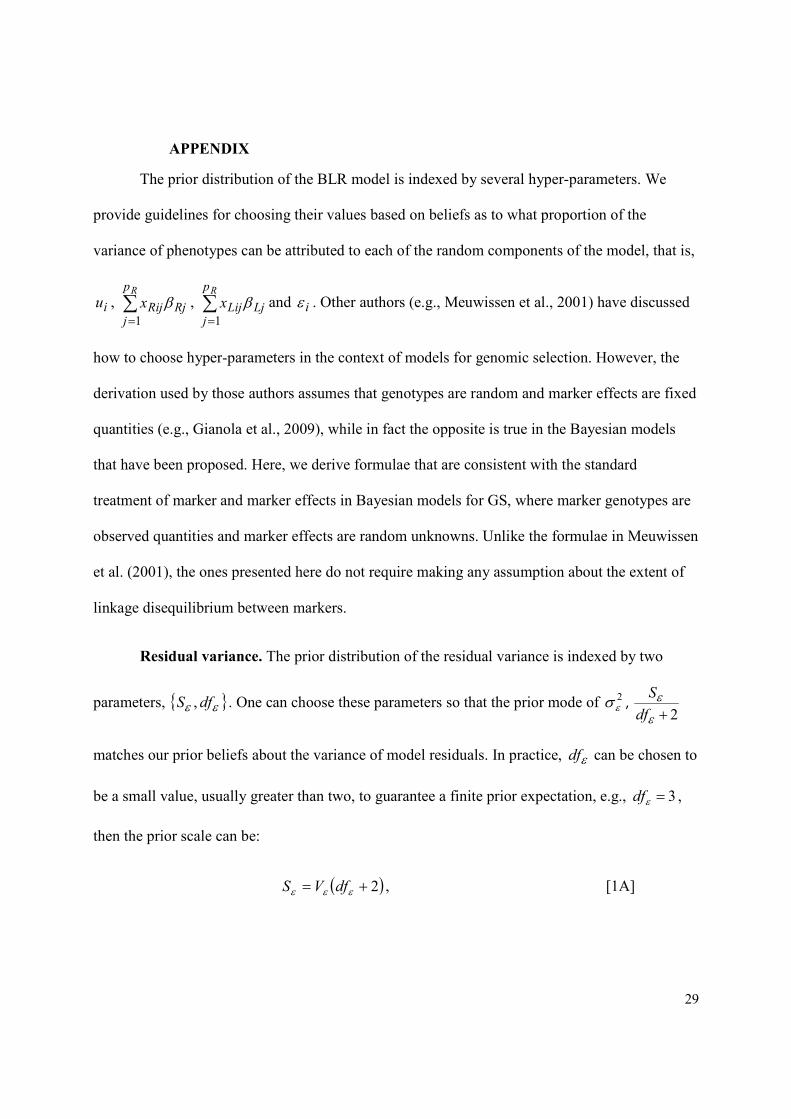
Residual variance. The prior distribution of the residual variance is indexed by two

parameters, { }εε dfS , . One can choose these parameters so that the prior mode of 2εσ ,

2+ε

εdf

S

matches our prior beliefs about the variance of model residuals. In practice, εdf can be chosen to

be a small value, usually greater than two, to guarantee a finite prior expectation, e.g., 3=εdf ,

then the prior scale can be:

( )2+= εεε dfVS , [1A]

30

where εV is chosen to reflect our expectation of the variance of model residuals. Formulas

similar to that presented in this Appendix can be derived using formulas for the prior

expectation.

Variance of the infinitesimal effect. From the prior distribution, the variance of iu is

2uiia σ , where iia

is the ith

diagonal element of A, which in the absence of inbreeding equals one.

If we let a be the average diagonal value of A and uV be our prior expectation about 2uaσ , then

we can choose 3=udf and set the prior scale to be:

( )a

dfVS uu

2+= ε . [2A]

Prior variance of marker effects. The contributions of RX and LX to phenotypes is

∑=

.

1..

p

jjijx β . Here, (.) stands for R or L, depending on whether BRR or BL is being used. In

regressions for GS, marker genotypes are fixed and marker effects are random. Furthermore, at

the level of the marginal distribution, marker effects are IID; therefore,

( )jp

jijR

p

jjij VarxVxVar .

1

2.

1..

..

ββ ∑∑==

==

. For the ‘average’ genotype, this formula becomes

( )jp

jjR VarxV .

1

2.

.

β

= ∑=

, where jx. denotes the average value of the jth column of RX or LX .

In BRR, the prior distribution of marker effects is Gaussian and ( ) 2βσβ =RjVar . As

before, R

dfβ can be chosen to have a relatively small value, e.g., 3=R

df β , and then the prior

scale can be set to be

31

( )

∑

+×=

R

R

R p

jRj

R

x

dfVS

2

2ββ [3A]

where RV is set to reflect our expectation of the variance of phenotypes that can be attributed to

the regression on RX .

In the BL, the marginal prior density of marker effects is Double-Exponential, and the

prior variance of marker effects is ( ) 222 −= λσβ εLjVar . Plugging this in

( )jp

jjL

p

jjij VarxVxVar .

1

2.

1..

..

ββ

==

∑∑==

, we obtain 22

1

2. 2

.−

=

= ∑ λσ ε

p

jjL xV . Solving for λ , we get:

∑−=Rp

j

RjL xV 2122ˆεσλ [4A]

where 12 −LVεσ is a noise-to-signal variance ratio. With [4A] we can choose a target value for the

regularization parameter. Then we can choose hyper-parameters so that the prior has a mode and

is relatively flat, in the neighborhood of λ̂ .

The above formulas constitute guidelines for choosing values of hyper-parameters. In

practice, if Bayesian learning takes place, one would expect that the posterior distribution moves

away from the prior. Furthermore, with small n it is always useful to check the sensitivity of

inferences with respect to the choice of hyper-parameters.