GENETIC STRUCTURE OF ROCK BASS AND JOHNNY DARTERS:

IMPLICATIONS FOR GAMEFISH MANAGEMENT IN WISCONSIN

by

Lacie Jo Westbrook

Wisconsin Cooperative Fishery Research Unit

A Thesis

submitted in partial fulfillment of the

requirements for the degree of

MASTER OF SCIENCE

IN

NATURAL RESOURCES (FISHERIES)

College of Natural Resources

UNIVERSITY OF WISCONSIN

Stevens Point, Wisconsin

April 24, 2012

APPROVED BY THE GRADUATE COMMITTEE OF:

/~ Dr. nan Sl ss, Comrmttee Chmr U.S. Geological Survey

Wisconsin Cooperative Fishery Research Unit College ofNatural Resources

University of Wisconsin-Stevens Point Stevens Point, WI 54481

Dr. Dan Isermann College ofNatural Resources

University of Wisconsin-Stevens Point Stevens Point, WI 54481

College ofNatural Resources University of Wisconsin-Stevens Point

Stevens Point, WI 54481

Northern Lakes Ecologist Bureau of Science Services

Wisconsin Department ofNatural Resources Spooner, WI 54801

11

iii

ABSTRACT

Understanding the patterns of spatial genetic structure within and among

populations has become a critical component of fisheries management practices. The

hierarchical genetic structure of aquatic organisms is highly influenced by watershed

boundaries or other key geological features. Previous genetic research on walleye

(Sander vitreus) and muskellunge (Esox masquinongy) across their native range in

Wisconsin showed sampled populations in the Upper Chippewa River watershed were

more similar to fish from the neighboring Upper Wisconsin River watershed than they

were to fish in the lower reaches of the Chippewa River watershed. The discordance is

likely the result of glacial processes or widespread, cross-boundary stocking. The

underlying cause is important in implementing stock-based management of coolwater

gamefish in Wisconsin. The objective of this study was to determine if the previously

observed genetic structures for walleye and muskellunge populations in Wisconsin are

likely the result of zoogeographic processes or anthropogenic events. Three primary sub-

objectives were: (1) to determine if rock bass exhibit genetic structure among populations

in northern Wisconsin, (2) to determine if johnny darters exhibit genetic structure among

populations in northern Wisconsin, and (3) to determine if the genetic structures of rock

bass and johnny darter are consistent with the previously identified genetic structures of

walleye and muskellunge. The genetic structures were evaluated by sampling 22 rock

bass populations and 16 johnny darter populations in the five major watersheds in

northern Wisconsin. Genetic diversity was assessed with 10 microsatellite markers for

rock bass and 14 for johnny darters. A modified genetic stock identification (GSI)

method using a Bayesian hierarchical process for determining genetic structure across a

iv

landscape combined with analysis of molecular variance (AMOVA) was employed to

delineate genetic structure. Analysis of genetic structures of rock bass and johnny darters

revealed 14 and 16 unique genetic units, respectively. Because of limitations in

managing a large number of genetic units, putative management groups were identified

using AMOVA and a minimum ratio of among group variance (Va) to within-group

variance (Vb) of one. This approach identified nine genetic units for rock bass and eight

for johnny darters. The rock bass and johnny darter genetic structures were inconsistent

with the previously identified walleye and muskellunge genetic structures, but were

consistent with watershed boundaries. The current genetic structures of walleye and

muskellunge are most likely the result of past cross-watershed boundary stockings rather

than natural biogeography. Two management alternatives should be considered in the

future management of walleye and muskellunge in northern Wisconsin. The first option

is to manage based on the contemporary genetics and risk altering communities

downstream. The second alternative is to manage based on contemporary watershed

boundaries and risk altering populations that have already been altered through past

anthropogenic events.

v

ACKNOWLEDGEMENTS

Special thanks go out to the Wisconsin Department of Natural Resources and Sport Fish

Restoration Act for funding this research. I would also like to thank my graduate advisor,

Dr. Brian Sloss for all his guidance through the process, patience as I evolved not only in

the lab but also in the field, and help in teaching me that fish are not as bad as I initially

thought. I would like to acknowledge and profusely thank Andrea Musch for all her

guidance, help, support, and swimming lessons. Thanks to Ryan Franckowiak for

pushing me in the lab and in reading so I could become a better scientist. I would not

have been able to finish this project without all the equipment and facilities supplied by

the Wisconsin Cooperative Fishery Research Unit. I would also like to Dr. Michael

Bozek for being a mentor for the past two years. Thanks go out to Dr. Martin Jennings

for his insights in my sampling design and help in sample collection as well as being a

member of my committee. I would also like to thank various employees of the

Wisconsin Department of Natural Resources for collecting samples and providing me

information about rock bass and johnny darter populations. Thanks to Dr. Dan Isermann

and Dr. Tim Ginnett for being a part of my committee and for their insight and help.

Thanks to my field technicians Brandon Gilbertson and Adam Grunwald. Special thanks

to all the graduate students and undergraduates whose patience, encouragement, support

and knowledge helped me to gain perspective in science and evolve as a better person,

also for becoming my family and home away from home. Finally I would like to thank

my family for their understanding and patience when I didn’t make it home and for all

their support as I worked my way through this research. To my Mom and Dad for being

vi

supportive of my need to go where ever the wind blows me. To my sister whose life

advice was always welcome when days were hard and homesickness overwhelming.

vii

TABLE OF CONTENTS

TITLE PAGE ....................................................................................................................... i

COMMITTEE APPROVAL ............................................................................................... ii

ABSTRACT ....................................................................................................................... iii

ACKNOWLEDGEMENTS ................................................................................................ v

TABLE OF CONTENTS .................................................................................................. vii

LIST OF TABLES ............................................................................................................. ix

LIST OF FIGURES ........................................................................................................... xi

INTRODUCTION .............................................................................................................. 1

METHODS ......................................................................................................................... 8

Experimental Design ............................................................................................... 8

Sample Collection ................................................................................................. 10

DNA Extraction .................................................................................................... 10

Genetic Analysis ................................................................................................... 11

Statistical Analysis ................................................................................................ 11

Population-specific admixture analysis. ................................................... 13

Basic genetic structure .............................................................................. 14

Bayesian-admixture based genetic stock identification ............................ 15

Genetic and geographic distances. ........................................................... 16

Contemporary genetic management units ................................................ 17

Species comparisons ................................................................................. 17

RESULTS ......................................................................................................................... 19

Genetic Diversity .................................................................................................. 19

Genetic Stock Identification ................................................................................. 20

Basic genetic structure .............................................................................. 20

Bayesian genetic stock identification ........................................................ 22

Genetic and geographic distances ............................................................ 25

Contemporary genetic management units ................................................ 26

Species comparisons ................................................................................. 26

viii

DISCUSSION ................................................................................................................... 28

Genetic Structure of Rock Bass and Johnny Darters ............................................ 28

Species Comparisons ............................................................................................ 33

Management Implications ..................................................................................... 37

LITERATURE CITED ..................................................................................................... 41

ix

LIST OF TABLES

Table 1. Suite of microsatellite loci developed in-house for rock bass with description of

primer sequence, repeat motif, number of alleles (A), and allele range in numbers of

base pairs. .................................................................................................................. 48

Table 2. Suite of microsatellite loci developed in-house for johnny darters with

description of primer sequence, repeat motif, number of alleles (A), and allele range

in numbers of base pairs. .......................................................................................... 49

Table 3. Rock bass PCR reaction recipes, fluorescent labels, and thermocycler

temperature profiles for all multiplexes. Multiplex refers to the temperature profiles

listed as footnotes, 10x Buffer refers to 10x ThermoFisher PCR Buffer B without

MgCl2, dNTPs refers to final of deoxynucleotides at equal concentrations, and

MgCl2 refers to the concentration of 25mM magnesium chloride solution. All

reactions contained 0.5U of Taq DNA polymerase in 10 μL volumes and 40 ng

DNA/reactions. ......................................................................................................... 50

Table 4. Johnny darter PCR reaction recipes, fluorescent labels, and thermocycler

temperature profiles for all multiplexes. Multiplex refers to the temperature profiles

listed as footnotes, 10x Buffer refers to 10x ThermoFisher PCR Buffer B without

MgCl2, dNTPs refers to final concentration of deoxynucleotides at equal

concentrations, and MgCl2 refers to the concentration of 25mM magnesium chloride

solution. All reactions contained 0.5U of Taq DNA polymerase in 10 μL volumes

and 40 ng DNA/reactions.......................................................................................... 51

Table 5. Populations sampled for rock bass during the summer of 2010 and 2011.

Included are abbreviations for each population, county, Water Body Identification

Code (WBIC), latitude, longitude and current management unit. ............................ 52

Table 6. Rock bass diversity statistics (10 loci) for all sampled populations including

expected heterozygosity (He) and standard deviation (He SD), observed

heterozygosity (Ho) and standard deviation (Ho SD), mean number of alleles per

locus (A) and standard deviation (A SD), mean allelic richness (Ar) and total private

alleles (PA). Full population names are in Table 5. ................................................. 53

Table 7. Populations sampled for johnny darters during the summer of 2010 and 2011.

Included are abbreviations for each population, county, Water Body Identification

Code (WBIC), latitude, longitude and current management unit. ............................ 54

x

Table 8. Johnny darter diversity statistics (14 loci) for all sampled populations including

expected heterozygosity (He) and standard deviation (He SD), observed

heterozygosity (Ho) and standard deviation (Ho SD), mean number of alleles per

locus (A) and standard deviation (A SD), mean allelic richness (Ar) and total private

alleles. Full population names are in Table 7. ......................................................... 55

Table 9. Analysis of molecular variance (AMOVA) groupings for rock bass with sum of

squares (SS), percent of variation, p-values, and Va/Vb ratios. ................................ 56

Table 10. Analysis of molecular variance (AMOVA) groupings for johnny darters, sum

of squares (SS), percent of variation, p-values, and Va/Vb ratios. ............................ 57

Table 11. Rock bass population pairwise FST values from FSTAT v2.9.3.2 (below

diagonal) and significance values (above diagonal). Full population names are in

Table 5. ..................................................................................................................... 58

Table 12. Johnny darter population pairwise FST values from FSTAT v2.9.3.2 (below

diagonal) and significance values (above diagonal). Full population names are in

Table 7. ..................................................................................................................... 60

Table 13. Rock bass population pairwise Dest values from SMOGD v 1.2.5 (below

diagonal) and pairwise geographic distance in km (above diagonal). Full population

names are in Table 5. ................................................................................................ 61

Table 14. Johnny darter population pairwise Dest values from SMOGD v1.2.5 (below

diagonal) and pairwise geographic distance in km (above diagonal). Full population

names are in Table 7. ................................................................................................ 63

xi

LIST OF FIGURES

Figure 1. Contemporary management units for walleye and muskellunge based on Fields

et al. (1997). Bold lines denote management unit boundaries, dashed line represents

the split in the Chippewa River watershed for walleye into Upper Chippewa River

watershed and Lower Chippewa River watershed, and thin lines represent county

borders....................................................................................................................... 64

Figure 2. Genetic structure observed in walleye across the five major watersheds in

northern Wisconsin based on Hammen (2009) (Upper Wisconsin Unit; Purple,

Upper Chippewa Unit; Green, Lake Superior; Red). Genetic discordance was found

in walleye populations in the headwaters of the Chippewa River watershed. .......... 65

Figure 3. Genetic structure observed in muskellunge across the five major watersheds in

northern Wisconsin based on Spude (2010) (Upper Wisconsin Unit; Pink, Upper

Chippewa Unit; Yellow, Central Chippewa Unit; Blue). Genetic discordance was

found in muskellunge populations in the headwaters of the Chippewa River and

Wisconsin River watersheds. .................................................................................... 66

Figure 4. Sub-watersheds selected for sampling in northern Wisconsin during the

summer of 2010 and 2011. Yellow sub-watersheds represent target areas. Blue sub-

watersheds represent randomly selected areas. ......................................................... 67

Figure 5. Twenty-two sub-watersheds sampled for rock bass in northern Wisconsin

during the summers of 2010 and 2011. ..................................................................... 68

Figure 6. Sixteen sub-watersheds sampled for johnny darters in northern Wisconsin

during the summers of 2010 and 2011. ..................................................................... 69

Figure 7. Unrooted neighbor joining tree based on Cavalli-Sforza and Edwards (1969)

chord distance (Dc) for rock bass. Full population names are in Table 5.

Populations are color coded by watershed location (Blue = Wisconsin; Orange =

Chippewa; Black = Lake Superior; Purple = Lake Michigan; Green = St. Croix). .. 70

Figure 8. Unrooted neighbor joining tree based on Cavalli-Sforza and Edwards (1969)

chord distance (Dc) for johnny darters. Full population names are in Table 7.

Populations are color coded by watershed location (Blue = Wisconsin; Orange =

Chippewa; Black = Lake Superior; Purple = Lake Michigan; Green = St. Croix). .. 71

Figure 9. Mantel test comparing pairwise Dest values versus FST (θ) values for rock bass.

................................................................................................................................... 72

xii

Figure 10. Mantel test comparing pairwise Dest values versus FST (θ) values for johnny

darters. ....................................................................................................................... 73

Figure 11. Results from STRUCTURE v2.3.3 following the modified Coulon et al.

(2008) method of assignment for rock bass. Dashed boxes represent unreconciled

groups and solid boxes represent stable groupings at K=1. Populations with (+)

indicate most likely group but failed to assign with >75% probability and are

assumed to be individual units. ................................................................................. 74

Figure 12. Results from STRUCTURE v2.3.3 following the modified Coulon et al.

(2008) method of assignment for johnny darters. Dashed boxes represent

unreconciled groups and solid boxes represent stable groupings at K=1. Populations

with (+) indicate most likely group but failed to assign with >75% probability and

are assumed to be individual units. ........................................................................... 75

Figure 13. Mantel test comparing geographic distance (km) and genetic differentiation

(Dest) between all populations of sampled rock bass. ............................................... 76

Figure 14. Mantel test comparing geographic distance (km) and genetic differentiation

(Dest) between all populations sampled for johnny darters. ...................................... 77

Figure 15. (a) Nine resolved genetic units for rock bass. All sub-watersheds are color

coded to match units in which they grouped. (b) Composite map of walleye and

muskellunge genetic units as described in Figure 2 and 3. ....................................... 78

Figure 16. (a) Eight resolved genetic units for johnny darters. All sub-watersheds are

color coded to match units in which they grouped. (b) Composite map of walleye

and muskellunge genetic units as described in Figure 2 and 3. ................................ 79

1

INTRODUCTION

Understanding the patterns of spatial genetic structure within and among

populations has become a critical component of fisheries management practices. Genetic

structure can be defined as the distribution of genetic diversity across a landscape or the

non-random spatial distribution of genotypes resulting from different processes

(Vekemans and Hardy 2004). Species are seldom entirely panmictic and are typically

composed of subpopulations or stocks that are at least partially reproductively isolated

and differentiated from one another (Shaklee and Currens 2003). Just as species are

arranged into hierarchies of subpopulations, populations, metapopulations, etc., genetic

variation is often hierarchically structured (Heithaus and Laushman 1997). Genetic

diversity is most similar within populations and between geographically proximate

populations; as geographical distances between populations increase the degree of genetic

divergence also increases (Vekemans and Hardy 2004). Understanding and incorporating

this genetic structure can improve the efficacy of resource management practices. For

example, restrictions in temporal and spatial distribution along with partial reproductive

isolation provide a basis for local adaptation through natural selection and are the

foundation of the stock concept (Shaklee and Currens 2003).

The stock concept is a central theme in the management of nearly all fish and

shellfish species (Shaklee and Currens 2003). The concept is based on the premise that

productivity and evolutionary potential of a species is dependent on maintaining the

abundance and diversity of its component stocks (Shaklee and Currens 2003). A genetic

stock is defined as a population(s) of fish that occur in proximity to one another and share

sufficient genetic similarities to assume a common ancestor or sufficient migration to

2

allow adaptations to spread (Bryan and Larkin 1972; Shaklee and Currens 2003).

Members of a stock have similar biological and/or ecological attributes such as growth

rate, population dynamics, habitat selection, and food habits, that collectively warrant

their designation as unique stocks (Dizon et al. 1992; Carvalho and Hauser 1994).

Therefore, under the stock concept, effective management of a species is dependent on

understanding the number, distribution, and characteristics of all stocks so genetic and

ecological integrity, diversity, and abundance can be maintained (Dizon et al. 1992).

The Wisconsin Department of Natural Resources (WDNR) has identified several

fish management goals important for maintaining populations of gamefish, such as

walleye (Sander vitreus) and muskellunge (Esox masquinongy). These goals include

maintaining the genetic integrity of naturally reproducing populations (Hewett and

Simonson 1998; Simonson 2008). Genetic integrity can be defined as the relative

stability of genetic diversity within a population over time and is correlated with the

fitness of a population (Thelen and Allendorf 2001; Wang et al. 2002; Allendorf and

Luikart 2007). Conservation of locally adapted populations is important to maximize the

adaptive and evolutionary potential of a species (Lande and Shannon 1996; Hilborn et al.

2003). Because of the importance of genetic diversity, the conservation of genetic

integrity is a common goal of science-based management. The maintenance and

protection of genetic diversity within Wisconsin gamefish species requires knowledge of

the levels of diversity present in populations and its distribution or structure among

populations on the landscape; in short, a stock-based management system.

Previously, management units based primarily on watershed boundaries were

identified and currently serve as the basis of an approximate stock-based management

3

program. Fields et al. (1997) used multiple genetic marker systems and multiple species

to delineate management zones for fish species in the upper Midwest. This study

identified six genetic management zones for walleye and five for muskellunge in northern

Wisconsin (Figure 1; Fields et al. 1997). Despite poor resolution, the observed patterns

of diversity were mostly consistent with watershed boundaries within northern Wisconsin

(Fields et al. 1997). This finding was logical and, as such, these zones were prescribed

but considered tentative or preliminary because the study had relatively small sample

sizes, a low number of populations, and low genetic variability at the available genetic

markers (Fields et al. 1997). Hammen (2009) examined the contemporary genetic

structure of walleye in the Ceded Territory of Wisconsin (i.e., northern third of

Wisconsin; Staggs et al. 1990) using a more intensive sampling strategy and highly

polymorphic, microsatellite DNA loci. This study showed the genetic structure of

walleye differed from contemporary watershed management zones. A concurrent study

on muskellunge, resolved a genetic structure that deviated from contemporary watershed

management zones in a similar manner (Spude 2010). Although both studies found

general concordance of genetic structure and watershed boundaries within and among the

species, an obvious discordance existed between resolved genetic structure and watershed

boundaries in the headwater regions of the Upper Chippewa River watershed (Figures 2

and 3). Populations of both species in this region were consistently more similar to

populations in the headwaters of the adjacent Upper Wisconsin River watershed. Given

the large number of populations of gamefish in this region and the associated intensive

management activities on these populations, this discordance is a challenge to effective

stock-based management of these and other coolwater species.

4

Understanding the extent and identifying the fundamental cause(s) of the

discordance between these resolved genetic structures and contemporary watershed

boundaries remains important to fully implement a stock-based management program.

At least two possibilities merit evaluation: 1) the discordance is because of past stocking

events using sources/hatcheries that were more geographically proximate (i.e.,

convenient) as opposed to sources from the same genetic management unit, and 2)

geological events, likely glacial, that may have impacted the colonization and

establishment of native fishes in this region resulting in a pattern of diversity that

captures the geologic history as opposed to the current watershed boundaries. These two

possibilities have different implications for management decisions. One management

decision would rely on contemporary genetic diversity to delineate management units

regardless of watershed boundaries. Management based on such genetic units would

have to consider the implications of downstream migration into populations that belong

in a different genetic unit. Another possible decision would be to delineate management

units based solely on contemporary watershed boundaries. Risks with this approach

include potentially homogenizing diversity within a watershed despite the presence of

native heterogeneity.

Estimating the genetic structure of species that are not stocked or popular bait fish

could serve as a surrogate for estimating the natural genetic structure of fish species in

northern Wisconsin. This approach would minimize or even eliminate the potential

anthropogenic influences that may be driving key aspects of genetic structure in the two

previous gamefish genetic studies. Caro and O’Doherty (1999) described surrogate

species as a substitute, proxy, or focal organism used in place of another. The use and

5

practicality of surrogates is highly debated (Favreau et al. 2006). Some conservationists

claim the concept to be effective, efficient, or often the only practical way to continue

with research when little data is available (Favreau et al. 2006). Others have

demonstrated that the use of surrogates rarely correlates with many other species or taxa

(Favreau et al. 2006). In a few cases, surrogate species provided better coverage than

random threatened species and can provide helpful information as long as the objectives

of the use of surrogate species are clearly defined (Caro and O'Doherty 1999; Andelman

and Fagan 2000).

The use of surrogate species to estimate gamefish genetic structure in northern

Wisconsin is dependent on the availability of species that share a similar zoogeographic

history. The recession of the Wisconsonian glaciation (~12,000 years ago) produced the

watery landscape currently seen in northern Wisconsin (Pielou 1991). Several walleye

studies have shown that glacial refugia are key elements in shaping the genetic structure

of this species (Billington et al. 1992; Stepien and Faber 1998; McParland et al. 1999;

Strange and Stepien 2007). Assuming the majority of coolwater fish species recolonized

Wisconsin under a similar geographic and temporal model, these studies can be used to

infer recolonization of walleye and other fish species in this region. As the glaciers

receded, melt-water provided corridors between waterbodies for walleye, muskellunge

and other fish species (Knowles 2001).

Headwater capture is another geologic process that might have influenced the

genetic structure of aquatic species in northern Wisconsin. Headwater capture, also

known as river vicariance theory, is a geomorphological process through which stream

sections are displaced from one catchment to another (Burridge et al. 2007). As a result,

6

aquatic populations that genetically diverged from neighbor populations due, in part, to

geographical separation (genetic drift) are subsequently found in the same drainage

and/or river system. In this situation, apparent conflicts in the distribution of diversity or

genetic structure are observed. In fact, prime evidence of headwater capture events are

observed genetic relationships that are reflective of historical rather than contemporary

catchment boundaries (Burridge et al. 2007). Headwater capture can occur through

several means, including glaciation, flooding, mountain uplift, and continental drift.

Headwater capture can promote range expansion and vicariant isolation at the same time,

similar to glaciations, but over shorter geologic time scales than glaciation (Burridge et

al. 2007). In the case of walleye or muskellunge, waterways that are contemporarily

contiguous could have historically been part of different stream systems. If a geological

disturbance caused a change in the waterway, all fish located in that waterway would be

diverted into a new direction, possibly into a different watershed. Genetically, this

process can leave a signature similar to the discordance observed in the Wisconsin

walleye and muskellunge genetic structures.

In addition to zoogeographic considerations, the choice of logical surrogates

should focus on species that are ubiquitous and sympatric with both walleye and

muskellunge. Furthermore, the surrogate species should be relatively easy to sample in

large numbers. Rock bass (Ambloplites rupestris) and johnny darters (Etheostoma

nigrum) are both native species that are not stocked or used as bait fish, so anthropogenic

impacts on the genetic structure of these fish throughout their sympatric range with

walleye and muskellunge should be minimal.

7

The objective of this study was to determine if the previously observed genetic

structures for walleye and muskellunge populations in Wisconsin are likely the result of

zoogeographic processes or anthropogenic events. Three primary sub-objectives were

developed: (1) to determine if rock bass exhibit genetic structure among populations in

northern Wisconsin, (2) to determine if johnny darters exhibit genetic structure among

populations in northern Wisconsin, and (3) to determine if the genetic structures of rock

bass and johnny darter are consistent with the previously identified genetic structures of

walleye and muskellunge.

8

METHODS

Experimental Design

Four primary considerations were addressed in designing this study: 1) the species

to use as surrogates; 2) the number, location, and overall distribution of populations to be

sampled; 3) the number of samples collected from each population, and 4) the number

and type of molecular markers to use. Three criteria were used for selecting surrogates:

1) species had to be native to the study area of northern Wisconsin, 2) species could not

have been stocked, translocated, or used in the bait industry, and 3) species had to be

sympatric with walleye and muskellunge. As described previously, rock bass and johnny

darters were selected as surrogates for this study. Neither species is thought to have been

commonly used or targeted for use as bait. A review of WDNR propagation records from

1998-2009 (David Giehtbrock, WDNR unpublished data, personal communication)

showed only two lakes in Wisconsin with documented rock bass stockings/translocations.

Those lakes were not considered for inclusion in this study. The same review showed no

evidence of intentional translocation or stocking of johnny darters.

The number and distribution of sampled populations partially followed the design

of three previous studies focused on walleye and muskellunge genetic structure (Hammen

2009; Murphy 2009, and Spude 2010). Since the previous studies of walleye and

muskellunge were restricted to the northern third of Wisconsin this study was also

restricted to the same region (Figures 2 and 3). Because the major discordance between

genetic structure and watersheds were observed in the Upper Chippewa River/Upper

Wisconsin River headwaters, the primary target region of this study consisted of sub-

watersheds in and around those two headwaters. Five sub-watersheds on each side of the

shared border of the two watersheds were chosen as target areas (10 total sub-watersheds;

9

Figure 4). Two to three other sub-watersheds were randomly chosen in each of the five

major watersheds (Lake Superior, St. Croix River, Chippewa River, Wisconsin River,

and Lake Michigan) for a total of thirteen randomly chosen sub-watersheds (Figure 4).

Within the target sub-watersheds, preference was given to lakes previously sampled in

the walleye and muskellunge studies assuming they contained healthy populations of

either or both surrogate species. If no previously studied lakes were available in a given

sub-watershed or the population size of either species was limiting, the selection of lakes

was based on: (a) lakes listed by WDNR as having rock bass and/or johnny darters, and

(b) lakes with public access boat landings.

The minimum sample size of a population was dependent on the choice of

molecular markers for this study. Two species-specific suites of microsatellite markers,

specifically designed for this study, were chosen to predict genetic diversity and

structure. Microsatellites were chosen for several reasons including their high level of

polymorphism (Bernatchez and Duchesne 2000), the ability to assay their diversity via

PCR (Shaklee and Currens 2003), and the use of microsatellite markers in the previous

studies on muskellunge and walleye. The numbers of loci and sample size to collect are

dependent on each other and collectively relate to the expected levels of differentiation

between putative populations. A minimum of 10 and a maximum of 14 microsatellite

markers are commonly referenced as adequate for similar studies (Ruzzante 1998;

Hedrick 1999); however, this cannot be fully determined until after data have been

collected. A targeted minimum of 50 individuals of each species was sampled per lake as

recommended by Ruzzante (1998). The genetic data was analyzed using a series of tests

10

that hierarchically examined diversity and its partitioning into various groups; a process

commonly referred to as genetic stock identification (GSI; Shaklee and Currens 2003).

Sample Collection

Samples were collected via a combination of fyke netting, shoreline seining, and

electrofishing during the spring and summer of 2010 and 2011. Rock bass were sampled

non-lethally with genetic samples consisting of an anal fin clip stored in individually

labeled tubes and preserved with 95% non-denatured ethanol. When possible, measures

of weight (g), total length (mm) and sex were taken. Johnny darters were lethally

sampled by preserving whole fish in 95% non-denatured ethanol because fin clips

sufficient for repeated extractions would have likely been lethal to the majority of

sampled fish. Sampling techniques followed the Molecular Conservation Genetics

Laboratory’s (MCGL) standard operating protocol and received UWSP IACUC approval.

DNA Extraction

Genomic DNA from individual tissue samples were extracted using Promega

Wizard® Genomic DNA purification kit

1 (Promega Corp., Madison, WI) following a

standard operating procedure for a 96-well plate extraction. The extracted DNA was

quantified using a Nanodrop® ND-1000 spectrophotometer (Nanodrop Technologies,

Wilmington, DE). All DNA samples were normalized to a final concentration of 20

ng/µL before microsatellite amplification.

1 Use of trade and product names throughout does not constitute endorsement by the U.S. Government, the

Wisconsin Department of Natural Resources, or the University of Wisconsin-Stevens Point.

11

Genetic Analysis

A suite of 12 rock bass microsatellite loci and 14 johnny darter loci, developed in-

house using the methods of Glenn and Schable (2005), were used to characterize the

genetic diversity of the two species (Tables 1 and 2). Samples for each species were PCR

amplified using 5 multiplex reactions (per species) with fluorescently labeled primers

(Table 3 and 4). Amplicons were size fractionated on an ABI 3730 DNA Analyzer

(Applied Biosystems, Inc., Foster City, CA) with an in-lane standard (GenefloTM

625,

Chimerx, Inc., Milwaukee, WI) for accurate allele sizing. Allele sizes were determined

using GeneMapper® software (Applied Biosystems) and multilocus genotypes were

compiled using Microsoft Office Excel©

2010 v14.0.6 (Microsoft Corporation, Redmond,

WA). Because some samples would not yield complete genotypes despite multiple

efforts, an individual had to have a minimum of seven and ten successfully genotyped

loci to be included for rock bass and johnny darters, respectively. For quality assurance

and control, 10% of samples (randomly selected) were re-genotyped to estimate global

and locus-specific error rates.

Statistical Analysis

Genetic diversity.—Genetic diversity was determined using several different

measures including population specific allele frequencies, mean number of alleles per

locus (A), allelic richness (Ar), observed heterozygosity (Ho), and expected

heterozygosity (He). Microsatellite Toolkit v3.1.1 (Park 2001) was used to calculate

allele frequencies, Ho, He, and A. Differences in sample size are expected to impact

estimates of allelic diversity (A) (Leberg 2002; Kalinowski 2004), therefore, a rarefaction

method implemented in HP-RARE v1.0 (Kalinowski 2004) was used to calculate Ar and

12

the number of rarefacted private alleles per sampled population (alleles only found in a

single population).

Hardy-Weinberg equilibrium and linkage disequilibrium.—A genetic stock

identification (GSI) procedure was used to determine the genetic structure of each target

species across northern Wisconsin. The first step of GSI was to determine if all

populations conformed to Hardy-Weinberg equilibrium (HWE; Shaklee and Currens

2003). Hardy-Weinberg equilibrium is a critical factor in allowing allele frequencies to

be used to explain the genetic composition of the population(s) with deviations being

used to infer improper sampling techniques (Allendorf and Luikart 2007) or the presence

of genetic admixture (Wahlund effect; Wahlund 1928). Estimates of HWE were

performed using an exact test with a Markov Chain Monte Carlo (MCMC) method of

50,000 dememorization steps, 500 batches, and 50,000 iterations per batch (Guo and

Thompson 1992; Raymond and Rousset 1995b) as implemented in GENEPOP 4.0

(Rousset 2008). Alpha (αo = 0.05) was adjusted with a sequential Bonferroni correction

to account for multiple tests (Rice 1989). A common problem with HWE tests and

highly polymorphic loci (such as microsatellites) is a high Type-I error rate because of

the cumulative effect of rare expected genotypes (Pamilo and Varvio-Aho 1984). To

correct this problem, all significant HWE tests from the MCMC tests were re-tested

following the pooling of all genotypes with a frequency of <1% (Hedrick 1999). Re-

testing was performed using a chi-square goodness of fit test in Microsoft Office Excel®

2010 (Microsoft Corporation, Redmond, WA) and a sequential Bonferroni correction (αo

= 0.05; Rice 1989). Any populations that deviated significantly from HWE after

13

corrections were tested for null alleles, sequence stutter, or typographic/data entry errors

using the program MICRO-CHECKER v.2.2.3 (Oosterhout et al. 2004).

The next step in performing GSI was to assess the independence of the sampled

loci also known as linkage or gametic disequilibrium (Raymond and Rousset 1995a).

When a locus has allele frequencies that are not independent of another locus, the two

loci are in linkage disequilibrium and thus violate Mendel’s law of independent

assortment. The result is one of the two loci cannot be used in tests of genetic

differentiation among populations such as those used in GSI (Shaklee and Currens 2003;

Allendorf and Luikart 2007). GENEPOP 4.0 (Rousset 2008) was used to test for linkage

disequilibrium using Fisher’s exact tests with MCMC as described above. A sequential

Bonferroni correction was used to correct for multiple tests (Rice 1989).

Population-specific admixture analysis.—A confounding factor to the prediction

of genetic structure is the presence of admixed populations in a dataset. A Bayesian-

based clustering method was employed to test each sampled population for the presence

of admixture. Admixture analysis was performed in the program STRUCTURE

(Pritchard et al. 2000) using a burn-in of 50,000 cycles followed by 50,000 MCMC

repetitions with K (the number of potential genetic units) ranging from 1-4 with three

iterations to predict the number of genetic units contained in the sample. The ΔK method

from Evanno et al. (2005) was used in conjunction with the slope of the lnP(K) as

described by Pritchard et al. (2000) and Evanno et al. (2005) to predict the most likely

value of K, which requires finding the breakpoint in the slope of the distribution of

lnP(D) for different K values tested. LnP(D) is an estimate of the posterior probability of

the data for a given K. The asymptotic value of the posterior probabilities is assumed to

14

be associated with the correct K value in a given sample (Pritchard et al. 2000). Evanno

et al. (2005) showed the ΔK method detects the top level of population structure when

several hierarchical levels exist.

Basic Genetic Structure.—The first step in estimating the genetic structure of each

species was to construct a graphical representation of overall genetic divergence/structure

among populations from which predictions of genetic groups could be constructed. An

unrooted neighbor-joining (NJ) tree (Takezaki and Nei 1996) was constructured using

Cavalli-Sforza and Edwards chord distance (Dc; 1969) in PowerMarker v3.25 (Liu and

Muse 2005). Confidence in the topology was estimated using 10,000 bootstrap

pseudoreplicates from PowerMarker v3.25 and a majority rule consensus tree constructed

using CONSENSE from the PHYLIP package (Felsenstein 2005).

Analysis of molecular variance (AMOVA) was used to determine the significance

of the groups predicted from the NJ tree (Excoffier et al. 1992). AMOVA calculates the

total molecular variance for all sampled individuals and partitions the total variance into

among group variance (Va), among populations within groups variance (Vb), and within

population variance (Vc). Similar to ANOVA, AMOVA determines the significance of

each partition. All AMOVA tests were performed with 10,000 permutations and 5,000

pseudoreplicates (Lowe et al. 2004) using Arlequin v3.5.1.3 (Excoffier et al. 2005).

Ideally, the ultimate genetic structure scenario would show significant among group

variance (Va) while simultaneously recovering non-significant within group variance

(Vb). However, this occurs only when the number of groups approaches the number of

sampled populations so the ratio of Va/Vb was also calculated for all hypothetical groups

15

with the supposition that a biologically-relevant structure should, at a minimum, have a

Va/Vb ratio ≥1 (Spude 2010).

A final test of divergence using Wright’s (1931) fixation index (FST) was used to

test for the presence of additional structure within and among any and all final groups

after the AMOVA test. The FST analog, theta (θ), as recommended by Weir and

Cockerham (1984) for highly polymorphic genetic markers, was used to estimate the

fixation index. Pairwise population θ values were estimated in FSTAT v2.9.3.2 (Goudet

2001) and significance (deviation from zero) was tested with 5,000 bootstrap

pseudoreplicates. All groups that were identified with AMOVA and showed no

significant θ were determined to be genetically stable, likely biologically significant, and

candidates to be considered distinct populations and/or stocks. Because FST and its

analogs have been shown to deviate from linearity at moderate to high values, especially

with highly polymorphic microsatellite loci (Hedrick 2005), the divergence estimator Dest

(Jost 2008) was estimated. Pairwise population Dest values were estimated in SMOGD

v1.2.5 (Crawford 2010). The resulting matrix was tested for linearity versus the θ matrix

using a Mantel test with 9,999 iterations in GenAlEx v6.4 (Peakall and Smouse 2006).

Bayesian-admixture based genetic stock identification.—A modified GSI

approach was also used to estimate genetic structure of the rock bass and johnny darter

populations. An iterative genetic structure prediction approach modified from that used

by Coulon et al. (2008) was performed using the Bayesian admixture/structure prediction

method in STRUCTURE v2.3.3 (Pritchard et al. 2000). A series of steps was conducted

to identify the largest rate of change for K (ΔK) with the smallest variance and largest

probability. The iteration with the highest probability within the most likely K value is

16

then used to determine population groupings. Individuals within each population are

assigned a probability of belonging to a particular group (q) with all samples from that

population resulting in a mean q value (Q) representing a measure of overall genetic

composition for each population. The method of Coulon et al. (2008) uses an iterative

approach with an a priori threshold value of Q used to assign a population into a group.

For this study, the threshold for inclusion into a group was 75% (i.e., >75% of each

population’s genetic material assigned to a particular group). Populations with mean Q

<75% were assumed to be independent of the other populations within a given iteration

and, subsequently, their own gene pool. Similar to the previous description of

STRUCTURE-based admixture detection, three iterations of K ranging from 1-23 (rock

bass) or 1-17 (johnny darters) were performed with an initial burn-in period of 50,000

cycles followed by 50,000 MCMC repetitions. The most likely value of K for a given

group was predicted as described previously using the Pritchard et al. (2000) and Evanno

et al. (2005) approach. After each step of the process, new groups (consisting of sub-

groups) of each previously predicted group were constructed. Finally, an AMOVA, as

described previously, was used to test the significance of the smallest number of

presumed groupings.

Genetic and geographic distances.—Populations are expected to diverge across a

landscape through time because of limited connectivity and subsequent gene flow (Manel

et al. 2003). This isolation by distance (IBD) process can provide insight into the

patterns of divergence and, in some cases, the processes impacting this pattern. For

example, conformance to IBD suggests natural patterns of diversity whereas violation of

IBD could mean a disruption because of anthropogenic effects. The resolved genetic

17

structures of both species were tested for IBD using a Mantel test comparing a genetic

distance matrix (pairwise Dest as described previously) to a geographic distance matrix

(Manel et al. 2003). Pairwise geographic distances were calculated between centers of

each lake using the Point Distance feature in ArcGIS v9.3.1 (Environmental Systems

Resource Institute, Redlands, CA). The Mantel test was performed using GenAlEx v6.4

(Peakall and Smouse 2006) with 9,999 iterations.

Contemporary genetic management units.—The observed genetic structures of

both species were tested against the contemporary (watershed) genetic management units.

An AMOVA was performed with a priori groups of populations based on their watershed

membership. Analyses were conducted in Arlequin v3.1 (Excoffier et al. 2005) using the

methods previously described.

Species comparisons. —The purpose of this project is to determine if rock bass

and johnny darter genetic structures were consistent with walleye and muskellunge

genetic structure. Studies that involve quantitatively comparing genetic differences

between species are currently lacking. No studies could be found describing methods

that could be used to evaluate the genetic differences between walleye, muskellunge, rock

bass and johnny darters. To determine if genetic structures were consistent across

species, a comparative approach through geographical representation was used. Rock

bass and johnny darter genetic structures determined from the previous sections were

viewed visually by maps created in ArcGIS v9.3.1 (Environmental Systems Resource

Institute, Redlands, CA). Sampled sub-watersheds were color coded to match the genetic

units they grouped into. Then to determine if these genetic structures were consistent

with walleye and muskellunge GPS points, color coded for genetic units, of sampled

18

walleye and muskellunge populations were compared with rock bass or johnny darter

genetic structure maps individually. Maps were compared visually to determine

similarities.

19

RESULTS

In total, 1,092 rock bass were sampled from 22 of the 23 sub-watersheds targeted

for this study (Table 5; Figure 5). Sample sizes ranged from 28 to 72 with an average of

49.6 individuals (Table 6). Likewise, 784 johnny darters were collected from 16 of the

23 targeted sub-watersheds (Table 7; Figure 6). Other sampled sub-watersheds for

johnny darters yielded insufficient sample sizes to be used in the current study. Sample

sizes ranged from 30 to 58 with an average of 49 individuals (Table 8). One targeted

sub-watershed located in the Wisconsin River watershed was removed from the study

because of a lack of lakes with sufficient rock bass or johnny darter populations.

Genetic Diversity

All rock bass samples were initially analyzed at 12 microsatellite loci (Table 1).

Two loci (PanD02 and PanA74) were removed from the study due to inconsistencies in

amplification. Data from the remaining 10 loci were used for subsequent analyses. For

johnny darters, 14 microsatellite loci were amplified in 5 multiplex reactions (Table 4).

Genetic diversity varied considerably among the sampled populations for both

rock bass and johnny darters. Rock bass had relatively low levels of diversity across all

populations with a mean Ho of 0.4071, a mean He of 0.4000, and an observed A of 3.12

(Table 6). The variability in allelic richness was high with the largest difference between

Cranberry Lake (CRA) and Lake Noquebay (NOQ) at locus AruA46 (2.00 and 8.48,

respectively; Table 6). Rock bass private allelic richness followed similar patterns as the

other genetic diversity characteristics (Table 6).

Johnny darters had comparatively higher levels of genetic diversity with a mean

Ho of 0.6340, mean He of 0.6404, and observed A of 9.08 (Table 8). Allelic richness was

20

also higher in johnny darter than rock bass (Table 8). Total population values for private

allelic richness ranged from 0.69 (BIG) to 6.76 (HMO; Table 8).

Genetic Stock Identification

Hardy-Weinberg equilibrium and linkage disequilibrium.—Following sequential

Bonferroni correction, 3.4% (7 of 206) of rock bass locus by population comparisons

departed significantly from HWE. Loci PniB86 and PanB80 each showed two significant

differences from HWE expectations (PniB86: SAW and NOQ and Pan B80: WSL and

SPE), while AruA31, AruA55 and AruA63 were significant for one population each (PM,

BN, and MCK, respectively). When rare genotypes were pooled per Hedrick (2005),

AruA55 in BN was the only locus by population comparison that deviated from HWE

expectations. Because all remaining locus by population comparisons conformed to

HWE expectations (99.5%), it was concluded that the rock bass samples, as a whole,

conformed to HWE. The sampled rock bass also conformed to linkage equilibrium at all

990 tests following sequential Bonferroni correction. None of the sampled populations

for rock bass showed evidence of admixture.

A higher number of johnny darter locus by population comparisons (following

Bonferroni correction, 11.76%; 26 of 221) were significantly different from HWE

expectations. After rare genotypes were pooled per Hedrick (2005) no significant locus

by population tests were observed. Johnny darters also conformed to linkage equilibrium

at all 1,456 tests following sequential Bonferroni correction. None of the sampled

populations for johnny darters showed evidence for admixture.

Basic genetic structure.—The rock bass Dc unrooted NJ tree resolved a consistent

geographic split between the Chippewa River and Wisconsin River watersheds for rock

21

bass with a few exceptions (Figure 7). All sampled populations located within the

Wisconsin River watershed resolved to one group (Group A) and sampled populations

from the Chippewa River watershed grouped with the inclusion of two populations from

the Lake Superior watershed (GAL and LYN) and one population from the Lake

Michigan watershed (SPE) (Group B). Other populations sampled from the Lake

Michigan, St. Croix, and Lake Superior watersheds grouped although with low bootstrap

values (Group C). Confidence levels of internal nodes on the unrooted NJ tree were

generally low, resolving under the 60% moderate support level with the exception of

NOQ and SAW with 68.79% support and LCO and LHC with 68.66% support. The

results of AMOVA on the three putative rock bass groups (A, B, and C) showed

significant among group variance (10.98% variance; p < 0.0001) and within group

variance (13.80%; p < 0.0001) (Table 9a) suggesting further substructure existed.

The johnny darter Dc unrooted NJ tree resolved similar results as observed in rock

bass. Sampled johnny darter populations showed geographic splits roughly similar to

watershed boundaries. Populations sampled within the Wisconsin River watershed all

grouped with the inclusion of BUT and NOQ from the Lake Michigan watershed (Figure

8.) This group, without NOQ, had 89.86% bootstrap support. Populations sampled in the

Chippewa River watershed grouped with the inclusion of LYN from Lake Superior

watershed. Populations sampled in the Lake Superior and St. Croix watersheds were also

clustered. Overall, the resolution of internal nodes on the johnny darter unrooted NJ tree

was high. These three groups were used as the initial putative groups for AMOVA tests.

Significant among group variance (9.87%; p < 0.0001) and within group variance

22

(13.46%; p < 0.0001) was detected, suggesting further structure within the three groups

(Table 10a).

Pairwise FST (θ) comparisons for all populations in both rock bass and johnny

darters were significantly different from zero consistent with the presence of significant

genetic structure and a high number of genetic units (Tables 11 and 12). Mantel tests for

both rock bass and johnny darter samples examining the linearity of FST (θ) versus Jost’s

Dest (2008) showed significant linearity for both species (rock bass r2 = 0.7832, p < 0.001;

Figure 9; and johnny darter r2 = 0.8527, p < 0.001; Figure 10). However, an apparent

loss of linearity was observed as FST increased in the pairwise rock bass comparisons

(Figure 9). Therefore, Dest (instead of FST) was used for all further tests for both species

as a genetic distance measure. Pairwise Dest values for rock bass ranged from 0.00 (BIG

and WSL) to 0.39 (HMO and WSL; Table 11). Johnny darter Dest values ranged from

0.03 (BN and BIG) to 0.78 (LYN and MCK; Table 12).

Bayesian genetic stock identification.—The Bayesian GSI method showed

significant genetic structuring among the sampled rock bass and johnny darter

populations. For rock bass, two groups were initially identified with three populations

that failed to assign to a group with > 75% probability (Figure 11). Subgroup A was

consistent with populations sampled in the Wisconsin River watershed with the inclusion

of Half Moon Lake (HMO) and McKenzie Lake (MCK) located in the St. Croix River

watershed. Similar to the basic genetic structure, subgroup B consisted of all populations

from the Upper Chippewa River watershed with the inclusion of four Great Lakes

drainage populations. The final groupings resulted in 14 genetic units identified from the

22 originally sampled rock bass populations (Figure 11). Using these as a priori groups

23

for AMOVA, significant among group variance (15.54%, p < 0.0001) and within group

variance (8.09%, p < 0.0001) was detected with a Va/Vb ratio of 1.921 (Table 9b).

Managing a large number of genetic units is impractical; subsequently, the next

logical step was to determine if a smaller number of genetic units could be identified that

would meet the objective of conserving genetic diversity among groups of populations.

Each step of the iterative process was tested for significance with AMOVA and a Va/Vb

ratio ≥ 1. The genetic structure of rock bass, as suggested by the results of the Coulon et

al. (2008) method described previously, assigned the 22 populations into 14 groups.

Following the first iteration that utilized data from all 22 populations, two groups were

resolved. All populations located within the Wisconsin River watershed and including

two populations located in the St. Croix River watershed (HMO and MCK) assigned to a

Group 1(Figure 11). All populations located in the Chippewa River watershed, two

populations located in the Lake Superior watershed (LYN and GAL), and two

populations located in the Lake Michigan watershed assigned to Group 2 (Figure 11). A

few populations (NOQ, SOL, NEB) failed to assign to either group with > 75% Q-value

and were therefore treated as isolated, unique groups. This five genetic group iteration

(Group 1, Group 2, NOQ, SOL, and NEB) failed to recover an AMOVA Va/Vb ratio

greater than 1 suggesting further structuring (Va = 5.38%, p < 0.0001; Vb = 17.77%, p <

0.0001; Va/Vb = 0.303). The Wisconsin River watershed and St. Croix populations that

initially grouped as Group 1 were subsequently separated into two subgroups, Wisconsin

River watershed populations and St. Croix River watershed populations (Figure 11).

Now with six potential groups, subgroups 1a, 1b, Group 2 and the three independent

populations, AMOVA once again failed to report a Va/Vb ratio greater than 1 (Va =

24

9.84%, p < 0.0001; Vb = 14.15%, p < 0.0001; Va/Vb = 0.695). Group 2 could not be

further divided using the Bayesian approach, however, two populations located in the

Lake Michigan watershed, SPE and SAW, were distinctly different from the other

populations in the group. These two populations were placed in their own group and

AMOVA was reassessed with seven groups, subgroups 1a, 1b, subgroups 2a, 2b and

three independent populations. This grouping once again failed to report a Va/Vb ratio

greater than one, suggesting the presence of further genetic structuring (Va = 9.48, p <

0.0001; Vb = 13.93, p <0.0001; Va/Vb =0.681 ). Continuing with the iterative processes,

STRUCTURE separated subgroup 1b into individual groups, subgroup 1b1 and subgroup

1b2 and subgroup 2b was also separated into individual groups, subgroup 2b1 and

subgroup 2b2. Using these nine groups as a priori groupings for AMOVA, significant

among group variance (12.11%, p < 0.0001) and within group variation (11.72%, p <

0.0001) was detected and a Va/Vb ratio of 1.033 was achieved (Table 9c).

The Bayesian GSI method initially predicted eight groups for johnny darters. One

population (PRC) failed to assign to a group with > 75% probability, however, it most

closely resembled populations in subgroup B (Figure 12). Subgroup A was consistent

with populations located within the Wisconsin River watershed, and subgroup B was

consistent with the Chippewa River watershed showing a separation across watershed

boundaries. In total, 16 stable genetic units corresponding to the sampled populations

were identified (Figure 12); this was not testable via AMOVA because of a lack of within

group variation. Using a 14 group scenario (TOM and PM grouped and NEB and MCK

grouped) a significant among group variance (13.55%, p < 0.0001) and within group

variance (7.25%, p < 0.0001) was detected with a Va/Vb ratio of 1.869 (Table 10b)

25

Similar to rock bass, the genetic structure of johnny darters, as suggested by the

results of the Coulon et al (2008) method described previously, assigned the 16

populations into unique genetic units. Following the first iteration that utilized all 16

populations eight genetic units were determined with one population (PRC) failing to

resolve with > 75% probability to a group, but most closely resembling populations in

Group 5 (Figure 12). Group 1 consisted of populations located in the Wisconsin River

watershed. Groups 2 and 3 were individual populations both located in the Chippewa

River watershed. Group 4 consisted of populations located in two watersheds, the

Wisconsin River watershed and Lake Michigan watershed. Group 5 consisted of

populations located in the Chippewa River watershed and included PRC which it most

likely resembled. Group 6 was formed with two groups from the St. Croix River

watershed and one from the Lake Superior watershed. Groups 7 and 8 were individual

populations; one from the Lake Michigan watershed and one from the Lake Superior

watershed. The eight group scenario (leaving PRC in Group 5) from the first step of the

Bayesian GSI is most likely the smallest number of genetic units for johnny darters

(Figure 12). AMOVA testing showed significant among group variance (13.36%, p <

0.0001) and within group variance (8.79%, p < 0.0001) and also provided a Va/Vb ratio

greater than one (1.52; Table 10c).

Genetic and geographic distances.—Significant positive relationships existed

between pairwise genetic distances (Dest) and geographic distances for both species. The

geographic distance between sampled rock bass and johnny darter populations ranged

from 9.02 km (LYN and BIG) to 355.37 km (NOQ and HMO; Table 11). The Mantel

test showed a significant relationship between genetic and geographic distance in rock

26

bass (R2 = 0.126; p = 0.012; Figure 13) and johnny darters (R

2 = 0.145; p = 0.005; Figure

14).

Contemporary genetic management units.—Rock bass and johnny darter

populations were grouped according to the watershed in which they are located for

AMOVA testing. Five groups were created consisting of samples located in the Lake

Superior, St. Croix River, Chippewa River, Wisconsin River, and Lake Michigan

watersheds. For rock bass, significant among group variance (9.34%, p < 0.0001) and

within group variance (14.11%, p < 0.0001) was observed with and an overall Va/Vb of

0.662 (Table 9d). A similar pattern was found for johnny darters with a significant

among group variance (9.03%, p < 0.0001) and within group variance (13.19%, p <

0.0001) resulting in a Va/Vb ratio of 0.685 (Table 10d).

Species comparisons.—Maps were created in ArcGIS to visualize the predicted

genetic structures of rock bass and johnny darters. Since it is infeasible to manage based

on individual lakes, the smallest number of genetic units discovered (nine for rock bass

and eight for johnny darters) were used to color code the sub-watersheds that were

sampled (Figure 15 and 16). The nine rock bass genetic units show a separation between

most of the major watersheds in northern Wisconsin. All sampled populations located in

the Wisconsin River watershed distinctly group together with no overlap with sampled

populations in any other watershed. The sampled populations in the Chippewa River

watershed group together except for one population that resolved as its own genetic unit.

This group includes two populations from the Lake Superior watershed which are located

on the border of the Chippewa River watershed. All other sampled populations in the

other watersheds were determined to be individual genetic units.

27

The sampled johnny darter populations separated into eight distinct genetic units.

The genetic units showed a distinct separation between most of the watersheds. The

populations sampled in the Wisconsin River watershed grouped together with the

inclusion of one population located in the Lake Michigan watershed, but did not include

any populations from the Chippewa River watershed. The sampled populations in the

Chippewa River watershed separated into two genetic units but did not include

populations from any other watershed.

The patterns of genetic structure observed in rock bass and johnny darter were not

consistent with the previous studies of walleye and muskellunge. The walleye and

muskellunge studies determined three genetic units in northern Wisconsin with one

genetic unit over lapping two major watersheds, the Wisconsin River watershed and the

Chippewa River watershed. The current study did not find any genetic units that crossed

this boundary (Figure 15 and 16).

28

DISCUSSION

The goal of this study was to determine if the previously observed patterns of

genetic structure within walleye and muskellunge were the likely result of zoogeographic

processes or anthropogenic events. By using the genetic structure of two native

coolwater fishes that have not been stocked as surrogate patterns of natural genetic

diversity in Wisconsin, this study showed distinct differences between the previously

resolved walleye and muskellunge structure and the johnny darter and rock bass genetic

structure. The most stringent results of the modified GSI resolved 14 unique rock bass

gene pools (from 22 sampled populations) and the johnny darter populations all resolved

as unique gene pools (n = 16 populations). The smallest number of potential genetic

groups for rock bass and johnny darters revealed genetic structure consistent with

contemporary watershed management zones. Through close consideration and evaluation

of these two surrogate genetic structure patterns and subsequent comparison to the

previously resolved walleye and muskellunge genetic structures, a better understanding

of what processes have resulted in the observed genetic structures arises. These findings

were inconsistent with the resolved genetic structures of walleye and muskellunge,

suggesting past stocking events altered the genetic structures.

Genetic Structure of Rock Bass and Johnny Darters

Significant genetic differences occurred among the sampled rock bass populations

consistent with expectations based on geographic proximity and contemporary watershed

boundaries. Populations located in the Chippewa River watershed consistently showed

greater similarities to each other rather than when compared to other populations in the

29

other watersheds regardless of the analytical method. The ultimate resolution of the

remaining (13) populations as unique gene pools failed to account for the observed

geographical similarity throughout the hierarchical analysis. For example, the

populations from the Upper Wisconsin River consistently resolved separately from the

Upper Chippewa River populations and showed significant similarity in the AMOVA

analyses. Only when the full iterative approach (i.e., significant among group variance

and non-significant within group variance) was employed did the individual populations

resolve as unique.

The johnny darter populations resolved a similar, high degree of genetic structure

with all sampled populations representing unique gene pools. When the entirety of the

analytical process was considered, geographical structure was apparent at early phases of

the analysis consistent with watershed influence on the genetic structure. The primary

pattern observed in the data was a discrete separation of the Upper Chippewa River

populations from the Upper Wisconsin River populations.

The high degree of genetic structure was consistent with other microsatellite

studies of fish species throughout the Upper Midwest including walleye (Hammen 2009),

muskellunge (Spude 2010), lake sturgeon (Acipenser fulvescens; Welsh et al. 2008) ,

smallmouth bass (Micropterus dolomieu; Stepien et al. 2006), and white sucker

(Catostomus commersoni; Lafontaine and Dodson 1997). Stepien et al. (2006) found

little or no gene flow between separated lakes or between river drainages in smallmouth

bass populations in the Great Lakes region. They suggested the degree of differentiation

reflects patterns of colonization and populations have been separated by geographical

barriers among lakes and the basins in which they are located, constricting gene flow

30

between populations. On a small scale, genetic divergence was linked to low migration

and a tendency for behavioral site fidelity (Stepien et al. 2006). Within lakes, migration

was higher between sites and genetic divergence was tied to geographic distances. All of

these factors are likely occurring in rock bass and johnny darter populations used in this

study and the original walleye and muskellunge populations studied by Hammen (2009)

and Spude (2010), respectively. Of special consideration is the lack of natural migration

between isolated populations of coolwater species resulting, essentially, in aquatic

‘islands’ on the geographical landscape.

The hierarchical genetic structure observed in Wisconsin’s rock bass and johnny

darter populations are the likely result of numerous factors including life history,

landscape connectivity, and anthropogenic changes to the landscape. Since rock bass and

johnny darters are not translocated for stocking or bait, anthropogenic factors not related

to the landscape (i.e., direct management activities) are likely minimized or eliminated

from consideration as an influence. The life histories of rock bass and johnny darters are

conducive to the high level of observed genetic differentiation. Life history traits such as

generation time, life span and mobility have an impact of the genetic structure of a

species (Stepien et al. 2007). Certain life history traits can have an impact not only on

within population genetic diversity but also between population genetic diversity. Rock

bass and johnny darters have been classified as sedentary species that remain in limited

areas (Becker 1983) indicating the potential for genetic structuring through the lack of

migration among populations. Migration between populations helps to maintain genetic

diversity within connected populations allowing for potential adaptive traits to be shared

through populations. With a lack of migration, such as with rock bass and johnny darters,

31

populations are subject to genetic drift, a nonselective random process that changes allele

frequencies. Genetic diversity is most similar within populations and as geographical

distance between populations increases the degree of genetic divergence also increases

(Vekemans and Hardy 2004). The distance between sampled populations of rock bass

and johnny darters would be consistent with the degree of structuring since migration is

lacking between populations. The lesser migratory probability of rock bass and johnny

darters, coupled with shorter generation times likely enhances measures of genetic

divergence among populations compared to the heavily managed and comparatively

long-lived walleye and muskellunge.

Reproductive and parental care specificity may promote genetic divergence

among spawning groups (Stepien et al. 2006). Rock bass, much like smallmouth bass, a

related species, are territorial nest builders that are relatively less fecund when compared

to other freshwater fish species, annually producing 2,000-11,000 eggs (Becker 1983).

Females spawn with more than one male and the largest individuals of both sexes are the

most reproductively successful due to high mate selectivity (Wiegmann and Baylis 1995).

Genetic studies for smallmouth bass spawning success showed 5.4% of all spawning

males produce 55% of the total number of fall young of the year (Gross and Kapuscinski

1997). Johnny darters mate in much the same way. Males are territorial breeders

annually producing 30-200 eggs (Becker 1983). This mating system influences the

effective population size (Ne) of a population. The effective population size is defined as

the size of an idealized population with the same level of genetic drift as the population in

question and determines the rate of genetic drift (Allendorf and Luikart 2007). Effective

population size can be altered by unequal sex ratios, nonrandom number of progeny and

32

fluctuation in population size (Allendorf and Luikart 2007). When the effective

population size of a population decreases, genetic drift increases causing differentiation

between populations. Skewed sex ratios limit the evenness of the genetic contribution of

individuals to the next generation and therefore decrease Ne (Allendorf and Luikart

2007). Low fecundity and low progeny survival generally results as a greater proportion

of the progeny are coming from a smaller number of parents reducing the effective size

of the population (Allendorf and Luikart 2007).

Given the high degree of concordance between rock bass and johnny darter

genetic structure and contemporary watershed boundaries, recent geologic events (e.g.,

Wisconsonian glaciation) were likely critical determinants in the distribution and

dynamics of these two species. Geologic events during the Wisconsonian glaciation have

been considered critical in the diversification and zoogeography of Wisconsin fishes

(Wiley and Mayden 1985; Mandrak and Crossman 1992; Roe et al. 2008). Knowles

(2001) showed that glaciation played an important active role in diversification of

populations. During glacial periods, populations were displaced to allopatric refuges and

regional structuring of genetic variation can be seen (Knowles 2001). Migration of fish

species was likely higher during or immediately after the Wisconsonian glaciation

(Mandrak and Crossman 1992) because of retreats and expansions of glacial lobes.

During the last glaciation, approximately 12,000 years ago, Wisconsin was divided into

two regions, one covered by a continental ice sheet and the other, an area free of ice,

known as the driftless region (Martin 1965). The area of concern for muskellunge and

walleye is in the northern region of Wisconsin and can be characterized as a highland

region (Martin 1965). It is thought that the ice sheet made several partial or complete

33

withdrawals from the highland region, and during the Wisconsonian glaciation a large

area of the highland was left unglaciated (Martin 1965). The retreat and expansion also

influenced the availability of a species’ suitable habitat and caused major range changes

(Hewitt 1996). As the glacial lobes retreated, more suitable habitats opened up creating

range expansion for many species, including the majority of fish species in Wisconsin’s

waters.

Recolonization of aquatic habitats as the glaciers receded has been shown in

numerous species to largely influence the spatial distribution of genetic diversity

(Underhill 1986; Billington et al. 1992; Mandrak and Crossman 1992). Recolonization of

Wisconsin’s coolwater fish community likely occurred relatively quickly because the

landscape was riddled with numerous (since lost) glacial melt water-fed bodies of water

and connections between these waters were numerous (Clayton and Moran 1982;

Underhill 1986). Past studies have shown that glacial refugia are key elements in shaping

the genetic structure of walleye (Billington et al. 1992; Stepien and Faber 1998; Strange

and Stepien 2007). These dispersal routes shifted, receded, and eventually were

eliminated, cutting off migration between populations.

Species Comparisons

Rock bass and johnny darter genetic structures were not consistent with the

genetic structures resolved for walleye and muskellunge. Although the 22 sampled rock

bass populations resolved into 14 distinct genetic units, hierarchical structure was

consistent with current watershed management units. A distinct separation between the

Chippewa River watershed and the Wisconsin River watershed was observed for both

34

species. No populations from either watershed were genetically similar to populations in

the other watershed. Such similarities were clearly observed in the previous walleye and

muskellunge studies (Hammen 2009; Spude 2010). The neighbor joining tree with three

initial groupings showed some lakes located in the Lake Superior watershed grouped with

lakes in the Upper Chippewa River watershed, but had clear separation between the

Chippewa and Wisconsin River watersheds (Figure 7). Big Lake located in the Upper

Chippewa River watershed was sampled for both rock bass and muskellunge. This lake

was determined to have a genetic similarity to the Upper Wisconsin River watershed for

muskellunge, but distinctly grouped with the Upper Chippewa River watershed for rock

bass. Isolation by distance (IBD) patterns for rock bass showed populations within close

geographic proximity to each other, but across watershed boundaries, in the targeted

sample area were more genetically differentiated than populations in the same watershed

in close proximity (Table 11, Figure 13). For example, Plum Lake (PM) and White Sand

Lake (WSL) were located 23.23 km apart in opposite watersheds and had a Dest value of

0.088. Tomahawk Lake (TOM) and Plum Lake (PM) were located 22.43 km apart in the

same watershed and had a Dest value of 0.014 (Table 11). Although only a single

comparison, it illustrates a nearly 6-fold increased level of divergence across watersheds

versus a within watershed comparison.

Similar pattern of watershed concordance, in contrast to the walleye and

muskellunge studies, was observed in the sampled johnny darter populations. All 16

populations resolved as distinct individual populations (i.e., gene pools); however, the

hierarchical structure was consistent with watershed boundaries. The neighbor joining

tree also resolved three distinct groups with discrete separations between the Wisconsin

35

River watershed and the Chippewa River watershed (Figure 8). The initial eight groups

from the Bayesian GSI showed populations in the Wisconsin watershed grouped together

and populations sampled in the Chippewa River watershed were distinctly different.

Isolation by distance patterns for johnny darters showed populations within close

geographic proximity to each other, but across watershed boundaries, in the targeted

sample area were more genetically differentiated than populations in the same watershed

in close proximity similarly to rock bass (Table 12, Figure 14). Lakes PM and WSL,

located in different watersheds but within 23.23km of each other, had a Dest value of 0.18

and lakes TOM and PM, located in the same watershed and 22.43km apart, had a Dest

value of 0.07 (Table 12).

The disjunct seen in walleye and muskellunge is most likely the result of past

stocking events. Given the genetic divergence of the previously studied walleye and

muskellunge populations and the introgressive behavior of fish, alteration of the gene

pool through cross watershed stocking is a plausible scenario (Campton and Johnston

1985; Cagigas et al. 1999; Franckowiak et al. 2009). Previous stocking events did not

always adhere to genetic or watershed boundaries. Historical stockings were often from

the most geographically proximate hatchery and not based on management units. The

Governor Tommy Thompson Hatchery and Art Oehmcke Hatchery have served as the

main hatcheries for muskellunge and walleye in the northern third of Wisconsin. Two

populations of muskellunge from the previous study (Spude 2010), located in the

Wisconsin River watershed, were determined to be more similar to populations located

within the Chippewa River watershed. These two populations had extensive stocking

records that showed stocking had taken place across watershed boundaries (Spude 2010).

36

It is likely that cross boundary stocking also occurred from the Wisconsin River

watershed to the Chippewa River watershed altering the genetic structure.

Despite the likely impact of cross-watershed stocking on the genetic structure of

walleye and muskellunge, this current study has some potential limitations that may limit

it’s applicability in interpreting all coolwater fish genetic structure. A possible limitation

to this present study was choosing two surrogate species whose life histories and mobility

are not more reflective of walleye and muskellunge. Rock bass and johnny darters have

limited mobility compared with walleye and muskellunge, which could have affected

dispersal patterns during colonization of the area. Perhaps the previously identified

walleye and muskellunge genetic structures represent different paths of recolonization or

times of dispersal during the last glaciations because of their ability to disperse farther

distances than rock bass and johnny darters in shorter amount of time. Johnny darters in

single lakes are sometimes limited by barriers that would be irrelevant to walleye and

muskellunge (Meixler et al. 2009). Some migration routes may have been more

conducive for larger fish and were barriers to smaller fish. Rock bass and johnny darter

populations may have been separated for a longer period of time than walleye and

muskellunge because of these differential migration impacts. Lack of migration and

increase in genetic drift for rock bass and johnny darter populations may have caused

changes in genetic structure to occur before walleye and muskellunge populations were

separated.

Another possible limitation of this study is that lakes sampled for rock bass and

johnny darters were not the same as the lakes sampled for walleye and muskellunge. The

current study design specifically used sub-watersheds instead of the lake specific

37

identifications. Therefore, the genetic structure could have been missed or differ between

the putative surrogates used in this study and the two coolwater species of interest. By

not sampling all the walleye and muskellunge lakes in the Upper Chippewa River

watershed that showed genetic similarities with the Upper Wisconsin River watershed,

the nature of the genetic structure for rock bass and johnny darters could not be known

and rock bass and johnny darters could in fact show similar disjuncts. When designing

this study, the assumption was made that if the genetic structure of walleye and

muskellunge was natural then it would be wide spread in the area. Sampling was based

on sub-watersheds for a broad sampling distribution of the area and to get a range of the

disjunct genetic structure of walleye and muskellunge. Also, other than the target area,

sub-watersheds were randomly chosen. The walleye and muskellunge sampled lakes

were based on WDNR survey lakes and tended to group together because of the close

proximity of lakes to each other in headwaters of the Chippewa River and Wisconsin

River watersheds. When possible, previously sampled lakes were sampled but not all

lakes showing disjunct patterns in past studies overlapped with a sub-watershed for this

study.

Management Implications

The Wisconsin DNR explicitly aims to manage walleye and muskellunge in ways

consistent with conserving the genetic integrity of self-sustained populations (Hewett and

Simonson 1998; Simonson 2008). The current management units for walleye and

muskellunge are based largely on watershed boundaries that likely reflect post-glacial

dispersal patterns and should contain genetically similar populations as reflected by this

38

study. To achieve these goals, sound biologically relevant management units need to be

followed. Contemporary watershed based management units are currently inconsistent

with the genetic structures of walleye and muskellunge; however, they are consistent with

the higher level genetic structures of rock bass and johnny darters observed in this study.

A key assumption of this study was that rock bass and johnny darter genetic structure

would represent a natural, ‘model’ genetic structure unaltered by anthropogenic events.

Based on this assumption, it is a logical conclusion that the lack of a strong watershed to

genetic relationship in walleye and muskellunge is most likely the result of past stocking

events that did not adhere to current watershed boundaries.

This study has resulted in two possible management actions: 1) manage walleye

and muskellunge based on current watershed boundaries or 2) manage based on the

contemporary genetic units determined in the previous studies. Continued reliance on the

current management units may not adequately protect the genetic integrity of individual

populations described in the previous studies since stocking has likely altered the genetic

structures. Managing on a unique gene pool basis is inefficient and infeasible.

Management units should be developed with the aim to minimize the genetic risks while

also considering the limitations of the management agency to manage a large number of

units. Limiting the number of genetic units would help improve efficiency by managing

a lower number of stocks and decreasing financial needs associated with management.

Continued management based on watershed boundaries is consistent with the

genetic structures observed in rock bass and johnny darters. Managing by watershed

boundaries would allow management units to remain the same. The number of lakes in

the Upper Chippewa River watershed that have been altered is unknown and this

39

management decision would eliminate the need to examine the genetic structure of every

lake in the watershed. Based on the walleye and muskellunge data, the primary

discordance is mostly isolated in the headwaters of the Upper Chippewa River; consistent

with populations in and around the Lac du Flambeau River system. However, continuing

to manage based on watershed boundaries does pose some risk to the current genetic

structures of walleye and muskellunge. Supplemental stocking of lakes that are more

genetically similar to a different watershed risks losing not only genetic diversity but also

similar biological and life history traits. Populations may be exposed to genetic

outbreeding. Genetic outbreeding and total gene pool replacement has been documented

in several species including walleye (Campton and Johnston 1985; Allendorf and Leary

1988; Sheridan 1995; Franckowiak et al. 2009). A study conducted on Escanaba Lake,

WI, by Franckowiak et al. (2009), looked at the temporal stability of the genetic diversity

of walleye and found almost total replacement of the original pool through supplemental

stocking. Genetic variation was comparable to the genetic variation in other populations

of walleye and genetic diversity did not decrease as would be expected with substantial

stocking.

The other management option would be to manage based on the contemporary

genetic units that were discovered in the walleye and muskellunge studies. This option

would preserve and prioritize the current genetic diversity and, ideally, integrity implying

that past historic structure cannot or should not be restored. This option assumes that

genetic integrity has already been altered by past stocking events, making the

preservation of what is on the landscape now crucial to keep from possibly losing genetic

diversity by further altering populations. This management option would most likely

40

conserve demographic characteristics that may be crucial to the fitness of the altered

populations and the common focus of primary management activities or monitoring.

Managing based solely on genetics, ironically, also poses potential genetic risks.

This option would require the knowledge of which specific populations belong to the

different genetic units. If populations are continually stocked across watershed

boundaries in accordance with their genetic unit, downstream populations connected

through waterways or flooding events would be at more-or-less continual risk from stray,

stocked individuals of a different genetic unit. Managing based on current genetic units

should be carefully managed so as to not alter the genetic integrity of downstream

populations. If these lakes have maintained unique gene pools, management should be

directed to reduce potential disruption. Supplemental stocking should only be applied to

these lakes when necessary and within their respective genetic units. However, managing

these lakes individually across watershed boundaries could become cumbersome in

determining which lakes have been altered. Time and financial costs, as is always the

case, will be considered by the responsible agencies in determining their optimal

approach to this challenge. The data presented herein will ideally provide a scientific

foundation for their informed decision making.

41

LITERATURE CITED

Allendorf, F. W., and R. F. Leary. 1988. Conservation and distribution of genetic

variation in a polytypic species, the cutthroat trout. Conservation Biology 2:170-

184

Allendorf, F. W., and G. Luikart. 2007. Conservation and the genetics of populations.

Blackwell Publishing, Malden, Massachusetts, USA.

Andelman, S. J., and W. F. Fagan. 2000. Umbrellas and flagships: Efficient conservation

surrogates or expensive mistakes? Proceedings of the National Academy of

Sciences of the United States of America 97:5954-5959.

Becker, G. C. 1983. Fishes of Wisconsin. University of Wisconsin Press Madison,

Madison, Wisconsin.

Beneteau, C. L., N. E. Mandrak, and D. D. Heath. 2007. Characterization of eight

polymorphic microsatellite DNA markers for the greenside darter, Etheostoma

blennioides (Percidae). Molecular Ecology Notes 7:641-643.

Bernatchez, L., and P. Duchesne. 2000. Individual-based genotype analysis in studies of

parentage and population assignment: How many loci, how many alleles?

Canadian Journal of Fisheries and Aquatic Sciences 57:1–12.

Billington, N., R. J. Barrette, and P. D. N. Hebert. 1992. Management implications of

mitochondrial DNA variation in walleye stocks. North American Journal of

Fisheries Management 12:276–284.

Bryan, J. E., and P. A. Larkin. 1972. Food specialization by individual trout. Journal of

the Fisheries Research Board of Canada 29:1615-1624.

Burridge, C. P., D. Craw, and J. M. Waters. 2007. An empirical test of freshwater

vicariance via river capture. Molecular Ecology 16:1883–1896.

Cagigas, M. E., E. Vazquez, G. Blanco, and J. A. Sanchez. 1999. Genetic effects of

introduced hatchery stocks on indigenous brown trout (Salmo trutta L.)

populations in Spain. Ecology of Freshwater Fish 8:141-150.

Campton, D. E., and J. M. Johnston. 1985. Electrophoretic evidence for a genetic

admixture of native and nonnative rainbow trout in the Yakima River,

Washington. Transactions of the American Fisheries Society 114:782-793

Caro, T. M., and G. O'doherty. 1999. On the Use of Surrogate Species in Conservation

Biology. Conservation Biology 13:805-814.

42

Carvalho, G. R., and L. Hauser. 1994. Molecular genetics and the stock concept in

fisheries. Reviews in Fish Biology and Fisheries 4:326–350.

Cavalli-Sforza, L. L., and A. W. F. Edwards. 1967. Phylogenetic analysis. Models and

estimation procedures. American Journal of Human Genetics 19:233.

Clayton, L., and S. R. Moran. 1982. Chronology of late Wisconsinan glaciations in

middle North America. Quaternary Science Reviews 1:55-82.

Coulon, A., J. W. Fitzpatrick, R. Bowman, B. M. Stith, C. A. Makarewich, L. M.

Stenzler, and I. J. Lovette. 2008. Congruent population structure inferred from

dispersal behaviour and intensive genetic surveys of the threatened Florida scrub-

jay. Molecular Ecology 17:1685-1701.

Crawford, N. G. 2010. SMOGD: Software for the measurement of genetic diversity.

Molecular Ecology Resources 10:556-557

Dizon, A. E., C. Lockyer, W. F. Perrin, D. P. Demaster, and J. Sisson. 1992. Rethinking

the Stock Concept: A Phylogeographic Approach. Conservation Biology 6:24-36.

Evanno, G., S. Regnaut, and J. Goudet. 2005. Detecting the number of clusters of

individuals using the software STRUCTURE: a simulation study. Molecular

Ecology 14:2611–2620.

Excoffier, L., G. Laval, and S. Schneider. 2005. Arlequin ver. 3.1: an integrated software

package for population genetics data analysis. Evolutionary Bioinformatics

Online 1:47–50.

Excoffier, L., P. E. Smouse, and J. M. Quattro. 1992. Analysis of molecular variance

inferred from metric distances among DNA haplotypes: application to human

mitochondrial DNA restriction data. Genetics 131:479-491.

Favreau, J. M., C. A. Drew, G. R. Hess, M. J. Rubino, F. H. Koch, and K. A. Eschelbach.

2006. Recommendations for assessing the effectiveness of surrogate species

approaches. Biodiversity and Conservation 15:3949–3969.

Felsenstein, J. 2005. PHYLIP (phylogeny inference package) version 3.6. Distributed by

the author. Department of Genome Sciences, University of Washington, Seattle.

Fields, R. D., M. D. G. Desjardins, J. M. Hudson, T. W. Kassler, J. B. Ludden, J. V.

Tranquilli, C. A. Toline, and D. P. Philipp. 1997. Genetic analysis of fish species

in the upper Midwest. Illinois Natural History Survey, Champaign, Illinois.

Franckowiak, R. P., B. L. Sloss, M. A. Bozek, and S. P. Newman. 2009. Temporal

effective size estimates of a managed walleye Sander vitreus population and

43

implications for genetic-based management. Journal of Fish Biology 74:1086-

1103.

Gabel, J. M., E. E. Dakin, B. J. Freeman, and B. A. Porter. 2008. Isolation and

identification of eight microsatellite loci in the Cherokee darter (Etheostoma

scotti) and their variability in other members of the genera Etheostoma,

Ammocrypta,and Percina. Molecular Ecology Resources 8:149-151.

Glenn, T. C., and N. A. Schable. 2005. Isolating microsatellite DNA loci. Methods in

enzymology 395:202–222.

Goudet, J. 2001. FSTAT, a program to estimate and test gene diversities and fixation

indicies (version 2.9.3).

Gross, M. L., and A. R. Kapuscinski. 1997. Reproductive success of smallmouth bass

estimated and evaluated from family-specific DNA fingerprints. Ecology

78:1424-1430.

Guo, S. W., and E. A. Thompson. 1992. Performing the exact test of Hardy-Weinberg

proportion for multiple alleles. Biometrics 48:361–372.

Hammen, J. J. L. 2009. Genetic structure of Wisconsin's naturally recuiting walleye

populations. Master's Thesis. University of Wisconsin-Stevens Point, Stevens

Point, Wisconsin.

Hedrick, P. W. 1999. Perspective: highly variable loci and their interpretation in

evolution and conservation. Evolution 53:313–318.

Hedrick, P. W. 2005. A standardized genetic differentiation measure. Evolution 59:1633-

1638.

Heithaus, M. R., and R. H. Laushman. 1997. Genetic variation and conservation of

stream fishes: influence of ecology, life history, and water quality. Canadian

Journal of Fisheries and Aquatic Sciences 54:1822-1836.

Hewett, S., and T. Simonson. 1998. Wisconsin's walleye management plan: moving

management into the 21st Century. STATISTICS.

Hewitt, G. M. 1996. Some genetic consequences of ice ages, and their role, in divergence

and speciation. Biological Journal of the Linnean Society 58:247–276.

Hilborn, R., T. P. Quinn, D. E. Schindler, and D. E. Rogers. 2003. Biocomplexity and

fisheries sustainability. Proceedings of the National Academy of Sciences

100:6564.

44

Jost, L. 2008. GST and its relatives do not measure differentiation. Molecular Ecology

17:4015-4026.

Kalinowski, S. T. 2004. HP-RARE 1.0: a computer program for performing rarefaction

on measures of allelic richness. Molecular Ecology Notes 5:187–189.

Knowles, L. L. 2001. Did the Pleistocene glaciations promote divergence? Tests of

explicit refugial models in montane grasshopprers. Molecular Ecology 10:691–

701.

Lafontaine, P., and J. J. Dodson. 1997. Intraspecific genetic structure of white sucker

(Catostomus commersoni) in northeastern North America as revealed by

mitochondrial DNA polymorphism.

Lande, R., and S. Shannon. 1996. The role of genetic variation in adaptation and

population persistence in a changing environment. Evolution 50:434–437.

Leberg, P. L. 2002. Estimating allelic richness: effects of sample size and bottlenecks.

Molecular Ecology 11:2445–2449.

Liu, K., and S. V. Muse. 2005. PowerMarker: an integrated analysis environment for

genetic marker analysis. Bioinformatics 21:2128.

Lowe, A., S. Harris, and P. Ashton. 2004. Ecological genetics: design, analysis, and

application. Wiley-Blackwell.

Mandrak, N. E., and E. J. Crossman. 1992. Postglacial dispersal of freshwater fishes into

Ontario. Canadian Journal of Zoology 70:2247-2259.

Manel, S., M. K. Schwartz, G. Luikart, and P. Taberlet. 2003. Landscape genetics:

combining landscape ecology and population genetics. Trends in Ecology &

Evolution 18:189–197.

Martin, L. 1965. Physical Geography of Wisconsin. University of Wisconsin Press,

Madison, WI.

Mcparland, T. L., M. M. Ferguson, and A. P. Liskauskas. 1999. Genetic population

structure and mixed-stock analysis of walleyes in the Lake Erie–Lake Huron

corridor using allozyme and mitochondrial DNA markers. Transactions of the

American Fisheries Society 128:1055-1067.

Meixler, M. S., M. B. Bain, and M. Todd Walter. 2009. Predicting barrier passage and

habitat suitability for migratory fish species. Ecological Modelling 220:2782–

2791.

45

Murphy, E. L. 2009. Contemporary muskellunge genetic structure resources in northern

Wisconsin: impacts of supplemental stocking and genetic management zones.

Master's thesis. University of Wisconsin-Stevens Point, Stevens Point, Wisconsin.

Oosterhout, C. V., W. F. Hutchingson, D. P. M. Wills, and P. Shipley. 2004. MICRO-

CHECKER: software for identifying and correcting genotyping errors in

microsatellite data. Molecular Ecology Notes 4:535-538.

Pamilo, P., and S. Varvio-Aho. 1984. Testing genotype frequencies and heterozygosities.

Marine Biology 79:99–100.

Park, S. D. E. 2001. Trypanotolerance in west African cattle and the population genetic

effects of selection. Ph.D. Thesis. University of Dublin.

Peakall, R., and P. E. Smouse. 2006. GENALEX 6: genetic analysis in Excel. Population

genetic software for teaching and research. Molecular Ecology Notes 6:288-295.

Pielou, E. C. 1991. After the ice age: the return of life to glaciated North America. The

University of Chicago Press, Chicago, IL.

Pritchard, J. K., M. Stephens, and P. Donnelly. 2000. Inference of population structure

using multilocus genotype data. Genetics 155:945-959.

Raymond, M., and F. Rousset. 1995a. An exact test for population differentiation.

Evolution 49:1280–1283.

Raymond, M., and F. Rousset. 1995b. GENEPOP (version 1.2): population genetics

software for exact tests and ecumenicism. Journal of heredity 86:248.

Rice, W. R. 1989. Analyzing tables of statistical tests. Evolution 43:223–225.

Roe, K. J., R. L. Mayden, and P. M. Harris. 2008. Systematics and zoogeography of the

rock basses (Centrarchidae: Ambloplites). Copeia 2008:858–867.

Rousset, F. C. O. 2008. Genepop'007: a complete re-implementation of the genepop

software for Windows and Linux. Molecular Ecology Resources 8:103–106.

Ruzzante, D. E. 1998. A comparison of several measures of genetic distance and

population structure with microsatellite data: bias and sampling variance.

Canadian Journal of Fisheries and Aquatic Sciences 55:1-14.

Shaklee, J. B., and K. P. Currens. 2003. Genetic stock identification and risk assessment.

Pages 291-328 in E. M. Hallerman, editor. Population genetics: principles and

applications for fisheries scientists, 2nd edition. American Fisheries Society,

Bethesda.

46

Sheridan, A. K. 1995. The genetic impacts of human activities on wild fish populations.

Reviews in Fisheries Science 3:91-108

Simonson, T. 2008. Muskellunge management update. Wisconsin Department of Natural

Resources.

Spude, B. T. 2010. Contemporary stock structure of muskellunge populations in northern

Wisconsin. Master's Thesis. University of Wisconsin-Stevens Point, Stevens

Point, Wisconsin.

Staggs, M. D., R. C. Moody, M. J. Hansen, and M. M. Hoff. 1990. Spearing and sport

angling for walleye in Wisconsin's ceded territory. Wisconsin Department of

Natural Resources, Fisheries Management Administrative Report 31, Madison,

Wisconsin.

Stepien, C. A., and J. E. Faber. 1998. Population genetic structure, phylogeography and

spawning philopatry in walleye (Stizostedion vitreum) from mitochondrial DNA

control region sequences. Molecular Ecology 7:1757-1769.

Stepien, C. A., D. J. Murphy, and R. M. Strange. 2007. Broad-to fine-scale population

genetic patterning in the smallmouth bass Micropterus dolomieu across the

Laurentian Great Lakes and beyond: an interplay of behaviour and geography.

Molecular Ecology 16:1605–1624.

Strange, R. M., and C. A. Stepien. 2007. Genetic divergence and connectivity among

river and reef spawning groups of walleye (Sander vitreus vitreus) in Lake Erie.

Canadian Journal of Fisheries and Aquatic Sciences 64:437–448.

Takezaki, N., and M. Nei. 1996. Genetic distances and reconstruction of phylogenetic

trees from microsatellite DNA. Genetics 144:389.

Thelen, G. C., and F. W. Allendorf. 2001. Heterozygosity-fitness correlations in rainbow

trout: effects of allozyme loci or associative overdominance? Evolution 55:1180–

1187.

Underhill, J. C. 1986. The fish fauna of the Lauentian Great Lakes, the St. Lawrence

Lowlands, Newfoundland, and Labrador. Pages 105-136 in C. H. Hocutt, and E.

O. Wiley, editors. The Zoogeography of North American Freshwater Fishes. John

Wiley and Sons, New York, New York.

Vekemans, X., and O. J. Hardy. 2004. New insights from fine-scale spatial genetic

structure analyses in plant populations. Molecular Ecology 13:921–935.

Wahlund, S. 1928. Zusammensetzung von Populationen und Korrelationserscheinungen

vom Standpunkt der Vererbungslehre aus betrachtet. Hereditas 11:65-106.

47

Wang, S., J. J. Hard, and F. Utter. 2002. Genetic variation and fitness in salmonids.

Conservation Genetics 3:321–333.

Weir, B. S., and C. C. Cockerham. 1984. Estimating F-statistics for the analysis of

population structure. Evolution 38:1358–1370.

Welsh, A., T. Hill, H. Quinlan, C. Robinson, and B. May. 2008. Genetic assessment of

lake sturgeon population structure in the Laurentian Great Lakes. North American

Journal of Fisheries Management 28:572-591

Wiegmann, D. D., and J. R. Baylis. 1995. Male body size and paternal behaviour in

smallmouth bass, Micropterus dolomieu (Pisces: Centrarchidae). Animal

Behaviour 50:1543-1555.

Wiley, E. O., and R. L. Mayden. 1985. Species and speciation in phylogenetic

systematics, with examples from the North American fish fauna. Annals of the

Missouri Botanical Garden 72:596-635.

Wright, S. 1931. Evolution in Mendelian populations. Genetics 16:97-159

48

Table 1. Suite of microsatellite loci developed in-house for rock bass with description of

primer sequence, repeat motif, number of alleles (A), and allele range in numbers of base

pairs.

Locus ID Primer Sequence (5'-3') Repeat Motif A Range (bp)

AruA31 F:HEX-TTGAATGCGCTTAACAGTGTG (AC)10 5 117-131

R:TTCACCCCAACTGAACTTCC

AruA46 F:HEX-TTTCCACTCTGCTCTCTGACTG (CA)16 14 196-226

R:TCCACATCGCTGTGAATCAG

AruA55 F:HEX-CCTCAGACATGACACACAAGC (AC)21 6 165-181

R:GCAAATCTCAGCAGGTAGCC

AruA63 F:GCATACGTTCAGACACCAAGG (AC)12 4 154-162

R:HEX-CTCAGGAGCTGCAGGACAG

AruB29 F:NED-CTGCTTTTGCAGCCTACTCC (CA)11 5 127-151

R:ATCAGCTGGGGAGATTGTTG

AruB38 F:6FAM-TGATTGCCAAGATTGACAGC (AG)28 14 128-158

R:TGTTGTTCGCCTATCTGTCC

AruC39 F:6FAM-GAGCCTGAACTGTCGGGTAG (AC)18 7 185-209

R:GATAGCAAAACATGCATGGAG

AruC58 F:NED-TGTTGACACCCATTCACTGC (TGTT)7 3 110-122

R:GGAGGGAGAGACAAGAGCTTC

PanA74 F:GCCAAGTCAATAATGACACTC (GT)11 10 137-163

R:6FAM-AGCATAGAACCCACAATGTC

PanB80 F:GGCCTAAATTGGTTTGTGAG (AC)9 14 156-198

R:NED-ATGTGGGGATCTTCAACAAC

PanD02

* F:GGTGATTGAAGTCATTGTAGC (GT)14 8 97-111

R:HEX-CCTGTTTCGGAGTATAACTG

PniB86

* F:6FAM-TTTGGTGTCTGTCAGCTATG (GT)11 10 130-154

R:TTAAGGAGCCTTGCTACATC

*Developed in-house for white and black crappie.

49

Table 2. Suite of microsatellite loci developed in-house for johnny darters with

description of primer sequence, repeat motif, number of alleles (A), and allele range in

numbers of base pairs.

Locus ID Primer Sequence (5'-3') Repeat Motif A Range (bp)

EniA15 F:HEX-TCATATTGGCAAGTGGATGG (CA)26 20 225-273

R:GCAGTAAAGCCAGGAAGTGC

EniA33 F:NED-AGCTGAACAATGCTGACCTG (TG)20 17 111-149

R:AGACAGCTTCACAGCCATGC

EniA93 F:HEX-TTGCACATATGGACGGACAC (AC)8 7 95-127

R:GCTAATGACTGCCACCAACC

EniB46 F:HEX-TGTATGTGGTGCATGTGTGG (TG)10 14 187-221

R:GGACTTGCAATTGTGTTGATG

EniC02 F:NED-CTGCTCCCGGATTGTTCTG (TG)17 8 238-262

R:TGATGCTCGCATGAGTCAAC

EniC42 F:6FAM-GCTGGATGGTGTCTAGATGG (GT)13 11 124-148

R:GGAGTGAGCTGATGGTGTCC

EniC74 F:6FAM-ACTGAGCCCTGAAGAAGTCG (TC)23 25 193-245

R:GGTGCCAGTGAATGAGCAG

EniD53 F:6FAM-TCTACATGCCGATTGTCCAC (GAAA)22 21 204-294

R:TACTCAGGCTGGGACCAGAG

EniE12 F:NED-TGTGCAAGCTGCAGATCAAG (TG)26 17 197-239

R:CTGGAATAAGATGCAGCTACAATG

EniE23 F:6FAM-TCGGTCTCCTTTACCGTCAG (TC)15 18 222-292

R:GAAAGGTGCTGGTCAGGAAG

EniE71 F:6FAM-CACAAGGAATAGCTGGCTGTC (GACA)7 12 192-244

R:GACTACCTCGTGGCTCATGG

EniF02 F:HEX-AGTGCAGTGTGGGAACTGG (AGAC)11 15 151-207

R:GGACGTCTGACTTGCTCTCC

Ebl4

1 F:6FAM-TGTGACTGATATTTTGCTGCTG (TATC)7GT(TCTA)7 23 164-260

R:TGCATATCAAGATTCCCATTTG

Esc26b

2 F:HEX-CAATGCGCCACATTGAGAAGG (TAGA)27 33 151-287

R:GCACAACATATGTCGTTAAGCTCC

1. Locus developed by Beneteau et al. (2007).

2. Locus developed by Gabel et al. (2008).

50

Table 3. Rock bass PCR reaction recipes, fluorescent labels, and thermocycler

temperature profiles for all multiplexes. Multiplex refers to the temperature profiles

listed as footnotes, 10x Buffer refers to 10x ThermoFisher PCR Buffer B without MgCl2,

dNTPs refers to final of deoxynucleotides at equal concentrations, and MgCl2 refers to

the concentration of 25mM magnesium chloride solution. All reactions contained 0.5U

of Taq DNA polymerase in 10 μL volumes and 40 ng DNA/reactions.

Locus Multiplex

10X

Buffer

(Conc.)

dNTP

(Conc.)

MgCl2

(Conc.)

Forward

Primer

(Conc.)

Reverse

Primer

(Conc.) Label

AruA31 1 1.00x 0.06mM 1.3mM 0.18μM 0.18μM Hex

AruB38

0.15μM 0.15μM 6Fam

AruC39

0.10μM 0.10μM 6Fam

AruA46 2 1.00x 0.06mM 1.7mM 0.18μM 0.18μM Hex

PniB86

0.28μM 0.28μM 6Fam

AruC58

0.09μM 0.09μM NED

AruA55 3 1.00x 0.06mM 1.3mM 0.15μM 0.15μM Hex

AruB29

0.22μM 0.22μM NED

AruA63 4 1.00x 0.06mM 1.25mM 0.12μM 0.12μM Hex

AruB80

0.22μM 0.22μM NED

PanA74 5 1.00x 0.06mM 1.25mM 0.24μM 0.24μM 6Fam

PanD02 6 1.00x 0.06mM 1.25mM 0.22μM 0.22μM Hex

1. 94°C for 2 min., 35 cycles each at 94°C for 30 s., 57°C annealing for 30 s., then 72°C

for 30 s., and a final elongation at 72°C for 10 min.

2. 94°C for 2 min., 35 cycles each at 94°C for 30 s., 52°C annealing for 30 s., then 72°C

for 30 s., and a final elongation at 72°C for 10 min.

3. 94°C for 2 min., 35 cycles each at 94°C for 30 s., 57°C annealing for 30 s., then 72°C

for 30 s., and a final elongation at 72°C for 10 min.

4. 94°C for 2 min., 35 cycles each at 94°C for 30 s., 58°C annealing for 30 s., then 72°C

for 30 s., and a final elongation at 72°C for 10 min.

5. 94°C for 2 min., 35 cycles each at 94°C for 30 s., 57°C annealing for 30 s., then 72°C

for 30 s., and a final elongation at 72°C for 10 min.

6. 94°C for 2 min., 35 cycles each at 94°C for 30 s., 55°C annealing for 30 s., then 72°C

for 30 s., and a final elongation at 72°C for 10 min.

51

Table 4. Johnny darter PCR reaction recipes, fluorescent labels, and thermocycler

temperature profiles for all multiplexes. Multiplex refers to the temperature profiles

listed as footnotes, 10x Buffer refers to 10x ThermoFisher PCR Buffer B without MgCl2,

dNTPs refers to final concentration of deoxynucleotides at equal concentrations, and

MgCl2 refers to the concentration of 25mM magnesium chloride solution. All reactions

contained 0.5U of Taq DNA polymerase in 10 μL volumes and 40 ng DNA/reactions.

Locus Multiplex

10X

Buffer

(Conc.)

dNTP

(Conc.)

MgCl2

(Conc.)

Forward

Primer

(Conc.)

Reverse

Primer

(Conc.) Label

EniA93 1 1.00x 0.06mM 1.70mM 0.15μM 0.15μM Hex

EniC02

0.20μM 0.20μM NED

Ebl4

0.20μM 0.20μM 6Fam

EniA33 2 1.00x 0.06mM 1.9mM 0.13μM 0.13μM NED

Esc26b

0.15μM 0.15μM Hex

EniE23

0.13μM 0.13μM 6Fam

EniA15 3 1.00x 0.06mM 1.7mM 0.24μM 0.24μM Hex

EniC74

0.10μM 0.10μM 6Fam

EniB46 4 1.00x 0.06mM 1.7mM 0.10μM 0.10μM Hex

EniC42

0.09μM 0.09μM 6Fam

EniE12

0.34μM 0.34μM NED

EniF02 5 1.00x 0.06mM 2.2mM 0.09μM 0.09μM Hex

EniD53

0.20μM 0.20μM Hex

EniE71

0.22μM 0.22μM 6Fam

1. 94°C for 2 min., 35 cycles each at 94°C for 30 s., 55°C annealing for 30 s., then 72°C

for 30 s., and a final elongation at 72°C for 10 min.

2. 94°C for 2 min., 35 cycles each at 94°C for 30 s., 55°C annealing for 30 s., then 72°C

for 30 s., and a final elongation at 72°C for 10 min.

3. 94°C for 2 min., 35 cycles each at 94°C for 30 s., 57°C annealing for 30 s., then 72°C

for 30 s., and a final elongation at 72°C for 10 min.

4. 94°C for 2 min., 35 cycles each at 94°C for 30 s., 57°C annealing for 30 s., then 72°C

for 30 s., and a final elongation at 72°C for 10 min.

5. 94°C for 2 min., 35 cycles each at 94°C for 30 s., 57°C annealing for 30 s., then 72°C

for 30 s., and a final elongation at 72°C for 10 min.

52

Table 5. Populations sampled for rock bass during the summer of 2010 and 2011. Included are abbreviations for each

population, county, Water Body Identification Code (WBIC), latitude, longitude and current management unit.

Lake Abbreviation County WBIC Latitude Longitude Management Unit

Bearskin Lake BEA Oneida 1523600 45.731 -89.685 Wisconsin

Big Lake BIG Vilas 2963800 46.154 -89.767 Chippewa

Butternut Lake BN Price/Ashland 2283300 45.983 -90.515 Chippewa

Cranberry Lake CRA Price 221700 45.621 -90.350 Chippewa

Deerskin Lake DEE Vilas 1601300 45.975 -89.171 Wisconsin

Half Moon Lake HMO Polk 2621100 45.498 -92.438 St. Croix

Lac Courte Oreilles LCO Sawyer 2390800 45.892 -91.438 Chippewa

Lake Galilee GAL Ashland 2935500 46.287 -90.602 Lake Superior

Lake Nebagamon NEB Bayfield 2858400 46.513 -91.703 Lake Superior

Lake Noquebay NOQ Marinette 525900 45.249 -87.924 Lake Michigan

Long/Herde Lake Chain LHC Chippewa 2351400 45.241 -91.416 Chippewa

Lynx Lake LYN Vilas 2954500 46.195 -89.666 Lake Superior

McKenzie Lake MCK Washburn 2706800 45.936 -92.046 St. Croix

Pelican Lake PEL Oneida 157990 45.503 -89.202 Wisconsin

Pike/Round Chain PRC Price 2268300/2267800 45.928 -90.067 Chippewa

Plum Lake PM Vilas 1592400 46.004 -89.514 Wisconsin

Sawyer Lake SAW Langlade 198100 45.247 -88.757 Lake Michigan

Solberg Lake SOL Price 2242500 45.749 -90.369 Chippewa

Somo Lake SOM Lincoln 1547700 45.516 -89.868 Wisconsin

Spread Eagles Chain SPE Florence 702100 45.901 -88.145 Lake Michigan

Tomahawk Lake TOM Oneida 1542700 45.830 -89.661 Wisconsin

White Sand Lake WSL Vilas 2321100 46.008 -89.827 Chippewa

53

Table 6. Rock bass diversity statistics (10 loci) for all sampled populations including expected heterozygosity (He) and standard

deviation (He SD), observed heterozygosity (Ho) and standard deviation (Ho SD), mean number of alleles per locus (A) and

standard deviation (A SD), mean allelic richness (Ar) and total private alleles (PA). Full population names are in Table 5.

Population Sample size He He SD Ho Ho SD A A SD Ar PA

TOM 48 0.4888 0.0371 0.5000 0.0228 3.10 1.73 2.96 1.74

PM 49 0.4897 0.0327 0.5143 0.0226 3.70 1.64 3.32 2.24

BEA 49 0.4666 0.0470 0.4612 0.0226 2.90 0.99 2.81 1.87

SOL 72 0.4416 0.0551 0.4345 0.0186 3.50 1.65 3.34 1.05

WSL 72 0.3178 0.0558 0.3132 0.0173 2.50 0.97 2.32 0.00

PEL 62 0.4329 0.0536 0.4210 0.0198 3.40 1.43 3.18 2.03

LYN 38 0.3703 0.0652 0.3831 0.0250 3.00 1.49 2.90 0.00

LCO 58 0.4242 0.0510 0.4138 0.0205 4.10 2.77 3.45 1.48

BIG 69 0.3614 0.0664 0.3695 0.0184 4.10 2.38 3.30 0.85

SAW 41 0.4330 0.0804 0.4360 0.0245 2.90 1.29 2.87 2.02

SOM 40 0.3454 0.0667 0.3545 0.0240 3.10 1.97 2.95 0.07

CRA 31 0.3742 0.0534 0.4273 0.0283 2.30 0.67 2.30 0.00

DEE 50 0.2847 0.0821 0.3123 0.0208 2.30 1.16 2.15 0.00

NOQ 50 0.4946 0.0729 0.5096 0.0224 4.20 2.57 3.94 3.03

SPE 43 0.3801 0.0706 0.3767 0.0234 2.90 1.52 2.76 0.90

BN 54 0.4465 0.0736 0.4344 0.0214 3.20 1.69 2.96 0.52

GAL 46 0.4552 0.0769 0.4630 0.0232 3.00 1.33 2.95 0.27

PRC 28 0.3792 0.0656 0.3964 0.0292 3.40 1.71 3.40 1.02

LHC 54 0.4108 0.0366 0.4211 0.0213 3.00 1.49 2.85 0.03

MCK 38 0.3281 0.0687 0.3142 0.0239 3.00 1.25 2.90 0.95

NEB 50 0.3658 0.0849 0.3832 0.0219 2.70 1.16 2.56 1.00

HMO 50 0.3090 0.0803 0.3171 0.0209 2.40 1.51 2.29 0.23

Mean 49.64 0.4000 0.0626 0.4071 0.0224 3.12 1.56 2.93 0.97

54

Table 7. Populations sampled for johnny darters during the summer of 2010 and 2011. Included are abbreviations for each

population, county, Water Body Identification Code (WBIC), latitude, longitude and current management unit.

Lake Abbreviation County WBIC Latitude Longitude Management Unit

Bearskin Lake BEA Oneida 1523600 45.731 -89.685 Wisconsin

Big Lake BIG Vilas 2963800 46.154 -89.767 Chippewa

Butternut Lake BUT Forest 692400 45.923 -88.986 Lake Michigan

Butternut Lake BN Price/Ashland 2283300 45.983 -90.515 Chippewa

Half Moon Lake HMO Polk 2621100 45.498 -92.438 St. Croix

Lac Courte Oreilles LCO Sawyer 2390800 45.892 -91.438 Chippewa

Lake Nebagamon NEB Bayfield 2858400 46.513 -91.703 Lake Superior

Lake Noquebay NOQ Marinette 525900 45.249 -87.924 Lake Michigan

Lynx Lake LYN Vilas 2954500 46.195 -89.666 Lake Superior

McKenzie Lake MCK Washburn 2706800 45.936 -92.046 St. Croix

Moen Chain MCK Oneida 1573800 45.660 -89.304 Wisconsin

Pike/Round Chain PRC Price 2268300/2267800 45.928 -90.067 Chippewa

Plum Lake PM Vilas 1592400 46.004 -89.514 Wisconsin

Solberg Lake SOL Price 2242500 45.749 -90.369 Chippewa

Tomahawk Lake TOM Oneida 1542700 45.830 -89.661 Wisconsin

White Sand Lake WSL Vilas 2321100 46.008 -89.827 Chippewa

55

Table 8. Johnny darter diversity statistics (14 loci) for all sampled populations including expected heterozygosity (He) and

standard deviation (He SD), observed heterozygosity (Ho) and standard deviation (Ho SD), mean number of alleles per locus (A)

and standard deviation (A SD), mean allelic richness (Ar) and total private alleles. Full population names are in Table 7.

Population Sample size He He SD Ho Ho SD A A SD Ar PA

LYN 44 0.4203 0.0871 0.4300 0.0201 4.21 2.99 4.03 2.03

SOL 54 0.5838 0.0692 0.5807 0.0179 5.64 2.76 5.30 2.35

BUT 53 0.5598 0.0670 0.5704 0.0183 6.57 2.98 5.67 3.40

NEB 30 0.6680 0.0566 0.6822 0.0229 8.00 4.17 7.89 1.61

BEA 54 0.6835 0.0511 0.6716 0.0172 8.14 3.96 7.49 0.61

MC 44 0.6293 0.0620 0.6249 0.0197 8.50 4.77 7.74 1.60

BIG 58 0.6233 0.0680 0.6182 0.0170 8.64 3.84 7.48 0.69

MCK 44 0.6459 0.0655 0.6349 0.0196 9.71 4.63 8.59 3.43

BN 43 0.6656 0.0585 0.6544 0.0195 9.71 5.09 8.50 2.15

PM 49 0.6967 0.0452 0.6759 0.0179 9.86 5.65 8.55 3.29

PRC 48 0.6476 0.0616 0.6154 0.0189 10.14 5.87 8.81 5.37

NOQ 49 0.6748 0.0535 0.6730 0.0180 10.14 4.61 8.71 4.75

HMO 50 0.6976 0.0410 0.6864 0.0176 10.64 3.88 9.06 6.76

TOM 50 0.6426 0.0585 0.6330 0.0183 10.79 5.63 9.28 1.27

WSL 56 0.6404 0.0632 0.6352 0.0172 11.29 6.11 9.18 2.97

LCO 58 0.7673 0.0348 0.7576 0.0152 13.36 6.58 10.70 7.06

Mean 49 0.6404 0.0589 0.6340 0.0185 9.08 4.59 7.94 3.08

56

Table 9. Analysis of molecular variance (AMOVA) groupings for rock bass with sum of squares (SS), percent of variation, p-

values, and Va/Vb ratios.

Grouping Scenario Source of Variation SS

% of

Variation p-value Va/Vb

(a) Three-group AMOVA from NJ Tree

Group A: LHC, SOL, LYN, LCO, BIG, PRC, CRA, BN,

WSL, GAL, SPE

Among Groups (Va) 465.887 10.98 <0.0001 0.797

Group B: PEL, BEA, SOM, DEE, TOM, PM Among Populations within Groups (Vb) 722.470 13.80 <0.0001

Group C: MCK, NEB, NOQ, SAW, HMO Within Populations (Vc) 4296.306 75.22 <0.0001

(b) 14-group AMOVA

Group 1: WSL, LYN, BIG, CRA, BN, GAL, PRC, LHC,

LCO

Among Groups (Va) 1005.893 15.54 < 0.0001 1.921

Group 2-14 (all individual groups): TOM, PM, DEE, PEL,

BEA, SOM, HMO, MCK, NEB, NOQ, SOL, SAW, SPE

Among Populations within Groups (Vb) 182.464 8.09 < 0.0001

Within Populations (Vc) 4296.306 76.37 < 0.0001

(c ) Nine-group AMOVA from Bayesian GSI

Group 1: TOM, PM, BEA, SOM, PEL, DEE Among Groups (Va) 769.36 12.11 < 0.0001 1.033

Group 2: BIG, BN, PRC, LCO, WSL, LYN, CRA, GAL,

LHC

Among Populations within Groups (Vb) 419 11.72 < 0.0001

Group 3-9 (all individual groups): HMO, MCK, SAW,

SPE, NOQ, NEB, SOL

Within Populations (Vc) 4296.31 76.18 < 0.0001

(d ) Contemporary Management Units AMOVA

Wisconsin River: TOM, PM, BEA, SOM, DEE, PEL Among Groups (Va) 534.386 9.34 < 0.0001 0.662

Chippewa River: BIG, WSL, LCO, PRC, SOL, CRA,

LHC, BN

Among Populations within Groups (Vb) 653.971 14.11 < 0.0001

Lake Superior: NEB, GAL, LYN Within Populations (Vc) 4296.306 76.56 < 0.0001

St. Croix: HMO, MCK

Lake Michigan: NOQ, SPE, SAW

57

Table 10. Analysis of molecular variance (AMOVA) groupings for johnny darters, sum of squares (SS), percent of variation, p-

values, and Va/Vb ratios.

Grouping Scenario Source of Variation SS

% of

Variation p-value Va/Vb

(a) Three-group AMOVA

Group A: TOM, PM, BEA, NOQ, BUT, MC Among Groups (Va) 704.229 9.87 < 0.0001 0.733

Group B: BIG, WSL, BN, LYN, SOL, LCO,

PRC Among Populations within Groups (Vb) 1043.605 13.46 < 0.0001

Group C: NEB, MCK, HMO Within Populations (Vc) 6828.294 76.68 < 0.0001

(b) 14-group AMOVA

Group 1: TOM, PM Among Groups (Va) 1670.398 13.55 < 0.0001 1.869

Group 2: NEB, MCK Among Populations within Groups (Vb) 77.436 7.25 < 0.0001

Group 3-14 (all individual populations): BEA, MC, LCO, PRC, SOL, WSL, BN, BIG,

NOQ, BUT, LYN, HMO

Within Populations (Vc) 6828.294 79.2 < 0.0001

(c) Eight-group AMOVA

Group 1: TOM, PM, BEA Among Groups (Va) 1320.028 13.36 < 0.0001 1.52

Group 2: BIG, WSL, BN Among Populations within Groups (Vb) 363.423 8.79 < 0.0001

Group 3: MC, BUT Within Populations (Vc) 6409.682 77.84 < 0.0001

Group 4: NEB, MCK, HMO

Group 5-8 (all individual populations): NOQ,

LYN, LCO, SOL

(d ) Contemporary Management Units

Wisconsin: TOM, PM, BEA, MC Among Groups (Va) 887.275 9.03 < 0.0001 0.685

Chippewa: BIG, WSL,BN, LCO, SOL, PRC Among Populations within Groups (Vb) 860.559 13.19 < 0.0001

Lake Superior: LYN, NEB Within Populations (Vc) 6828.294 77.79 < 0.0001

St. Croix: MCK, HMO

Lake Michigan: BUT NOQ

58

Table 11. Rock bass population pairwise FST values from FSTAT v2.9.3.2 (below diagonal) and significance values (above

diagonal). Full population names are in Table 5.

TOM PM BEA SOL WSL PEL LYN LCO BIG SAW SOM CRA

TOM *** <0.0001 <0.0001 <0.0001 <0.0001 <0.0001 <0.0001 <0.0001 <0.0001 <0.0001 <0.0001 <0.0001

PM 0.04 *** <0.0001 <0.0001 <0.0001 <0.0001 <0.0001 <0.0001 <0.0001 <0.0001 <0.0001 <0.0001

BEA 0.07 0.10 *** <0.0001 <0.0001 <0.0001 <0.0001 <0.0001 <0.0001 <0.0001 <0.0001 <0.0001

SOL 0.15 0.10 0.20 *** <0.0001 <0.0001 <0.0001 <0.0001 <0.0001 <0.0001 <0.0001 <0.0001

WSL 0.24 0.22 0.25 0.13 *** <0.0001 <0.0001 <0.0001 <0.0001 <0.0001 <0.0001 <0.0001

PEL 0.15 0.11 0.17 0.13 0.24 *** <0.0001 <0.0001 <0.0001 <0.0001 <0.0001 <0.0001

LYN 0.14 0.15 0.17 0.13 0.11 0.21 *** <0.0001 <0.0001 <0.0001 <0.0001 <0.0001

LCO 0.18 0.15 0.18 0.08 0.04 0.20 0.09 *** <0.0001 <0.0001 <0.0001 <0.0001

BIG 0.22 0.18 0.22 0.09 0.03 0.22 0.13 0.04 *** <0.0001 <0.0001 <0.0001

SAW 0.28 0.23 0.33 0.18 0.33 0.29 0.26 0.24 0.28 *** <0.0001 <0.0001

SOM 0.17 0.21 0.17 0.16 0.30 0.16 0.26 0.22 0.25 0.36 *** <0.0001

CRA 0.24 0.18 0.24 0.17 0.12 0.24 0.15 0.10 0.14 0.26 0.37 ***

DEE 0.28 0.20 0.27 0.30 0.37 0.23 0.26 0.29 0.35 0.37 0.42 0.32

NOQ 0.14 0.09 0.19 0.05 0.19 0.13 0.15 0.12 0.15 0.11 0.18 0.18

SPE 0.23 0.18 0.25 0.10 0.04 0.22 0.15 0.05 0.04 0.25 0.32 0.07

BN 0.18 0.14 0.20 0.11 0.14 0.19 0.13 0.08 0.08 0.21 0.24 0.16

GAL 0.15 0.11 0.20 0.06 0.14 0.20 0.12 0.05 0.12 0.19 0.25 0.13

PRC 0.23 0.18 0.24 0.10 0.07 0.19 0.10 0.03 0.08 0.23 0.28 0.09

LHC 0.24 0.20 0.25 0.11 0.14 0.25 0.17 0.06 0.09 0.21 0.26 0.19

MCK 0.22 0.19 0.33 0.16 0.41 0.30 0.37 0.30 0.34 0.29 0.28 0.42

NEB 0.22 0.21 0.30 0.15 0.33 0.32 0.31 0.21 0.25 0.25 0.29 0.36

HMO 0.38 0.31 0.45 0.33 0.52 0.36 0.47 0.43 0.45 0.32 0.49 0.45

59

Table 11. Continued.

DEE NOQ SPE BN GAL PRC LHC MCK NEB HMO

TOM <0.0001 <0.0001 <0.0001 <0.0001 <0.0001 <0.0001 <0.0001 <0.0001 <0.0001 <0.0001

PM <0.0001 <0.0001 <0.0001 <0.0001 <0.0001 <0.0001 <0.0001 <0.0001 <0.0001 <0.0001

BEA <0.0001 <0.0001 <0.0001 <0.0001 <0.0001 <0.0001 <0.0001 <0.0001 <0.0001 <0.0001

SOL <0.0001 <0.0001 <0.0001 <0.0001 <0.0001 <0.0001 <0.0001 <0.0001 <0.0001 <0.0001

WSL <0.0001 <0.0001 <0.0001 <0.0001 <0.0001 <0.0001 <0.0001 <0.0001 <0.0001 <0.0001

PEL <0.0001 <0.0001 <0.0001 <0.0001 <0.0001 <0.0001 <0.0001 <0.0001 <0.0001 <0.0001

LYN <0.0001 <0.0001 <0.0001 <0.0001 <0.0001 <0.0001 <0.0001 <0.0001 <0.0001 <0.0001

LCO <0.0001 <0.0001 <0.0001 <0.0001 <0.0001 <0.0001 <0.0001 <0.0001 <0.0001 <0.0001

BIG <0.0001 <0.0001 <0.0001 <0.0001 <0.0001 <0.0001 <0.0001 <0.0001 <0.0001 <0.0001

SAW <0.0001 <0.0001 <0.0001 <0.0001 <0.0001 <0.0001 <0.0001 <0.0001 <0.0001 <0.0001

SOM <0.0001 <0.0001 <0.0001 <0.0001 <0.0001 <0.0001 <0.0001 <0.0001 <0.0001 <0.0001

CRA <0.0001 <0.0001 <0.0001 <0.0001 <0.0001 <0.0001 <0.0001 <0.0001 <0.0001 <0.0001

DEE *** <0.0001 <0.0001 <0.0001 <0.0001 <0.0001 <0.0001 <0.0001 <0.0001 <0.0001

NOQ 0.26 *** <0.0001 <0.0001 <0.0001 <0.0001 <0.0001 <0.0001 <0.0001 <0.0001

SPE 0.34 0.14 *** <0.0001 <0.0001 <0.0001 <0.0001 <0.0001 <0.0001 <0.0001

BN 0.26 0.12 0.10 *** <0.0001 <0.0001 <0.0001 <0.0001 <0.0001 <0.0001

GAL 0.27 0.09 0.10 0.09 *** <0.0001 <0.0001 <0.0001 <0.0001 <0.0001

PRC 0.29 0.13 0.07 0.11 0.09 *** <0.0001 <0.0001 <0.0001 <0.0001

LHC 0.34 0.14 0.12 0.09 0.11 0.09 *** <0.0001 <0.0001 <0.0001

MCK 0.51 0.17 0.37 0.28 0.21 0.38 0.30 *** <0.0001 <0.0001

NEB 0.45 0.16 0.28 0.21 0.15 0.30 0.19 0.12 *** <0.0001

HMO 0.49 0.31 0.44 0.34 0.37 0.45 0.40 0.37 0.41 ***

60

Table 12. Johnny darter population pairwise FST values from FSTAT v2.9.3.2 (below diagonal) and significance values (above

diagonal). Full population names are in Table 7.

TOM BIG PM WSL SOL LCO MC BEA LYN PRC BN BUT NOQ NEB MCK HMO

TOM *** <0.001 <0.001 <0.001 <0.001 <0.001 <0.001 <0.001 <0.001 <0.001 <0.001 <0.001 <0.001 <0.001 <0.001 <0.001

BIG 0.24 *** <0.001 <0.001 <0.001 <0.001 <0.001 <0.001 <0.001 <0.001 <0.001 <0.001 <0.001 <0.001 <0.001 <0.001

PM 0.06 0.19 *** <0.001 <0.001 <0.001 <0.001 <0.001 <0.001 <0.001 <0.001 <0.001 <0.001 <0.001 <0.001 <0.001

WSL 0.20 0.08 0.16 *** <0.001 <0.001 <0.001 <0.001 <0.001 <0.001 <0.001 <0.001 <0.001 <0.001 <0.001 <0.001

SOL 0.24 0.11 0.20 0.15 *** <0.001 <0.001 <0.001 <0.001 <0.001 <0.001 <0.001 <0.001 <0.001 <0.001 <0.001

LCO 0.16 0.11 0.11 0.09 0.13 *** <0.001 <0.001 <0.001 <0.001 <0.001 <0.001 <0.001 <0.001 <0.001 <0.001

MC 0.12 0.31 0.11 0.28 0.31 0.21 *** <0.001 <0.001 <0.001 <0.001 <0.001 <0.001 <0.001 <0.001 <0.001

BEA 0.08 0.21 0.07 0.18 0.23 0.15 0.11 *** <0.001 <0.001 <0.001 <0.001 <0.001 <0.001 <0.001 <0.001

LYN 0.36 0.29 0.32 0.30 0.33 0.27 0.40 0.33 *** <0.001 <0.001 <0.001 <0.001 <0.001 <0.001 <0.001

PRC 0.14 0.10 0.11 0.13 0.12 0.11 0.22 0.14 0.33 *** <0.001 <0.001 <0.001 <0.001 <0.001 <0.001

BN 0.22 0.03 0.17 0.06 0.10 0.09 0.28 0.18 0.26 0.10 *** <0.001 <0.001 <0.001 <0.001 <0.001

BUT 0.17 0.33 0.18 0.29 0.35 0.22 0.12 0.16 0.39 0.27 0.30 *** <0.001 <0.001 <0.001 <0.001

NOQ 0.18 0.24 0.16 0.22 0.23 0.18 0.18 0.13 0.40 0.16 0.21 0.24 *** <0.001 <0.001 <0.001

NEB 0.24 0.24 0.18 0.21 0.27 0.16 0.26 0.17 0.41 0.21 0.21 0.30 0.20 *** <0.001 <0.001

MCK 0.22 0.27 0.19 0.25 0.28 0.17 0.24 0.17 0.43 0.21 0.25 0.28 0.19 0.11 *** <0.001

HMO 0.23 0.18 0.20 0.13 0.25 0.11 0.25 0.21 0.34 0.21 0.17 0.26 0.22 0.18 0.19 ***

61

Table 13. Rock bass population pairwise Dest values from SMOGD v 1.2.5 (below diagonal) and pairwise geographic distance in

km (above diagonal). Full population names are in Table 5.

TOM PM BEA SOL WSL PEL LYN LCO BIG SAW SOM CRA

TOM *** 22.43 11.07 55.97 21.72 50.93 40.61 138.12 36.92 95.74 38.38 57.92

PM 0.01 *** 33.02 72.22 23.23 60.70 24.29 149.59 25.65 102.74 60.75 77.17

BEA 0.04 0.03 *** 53.52 30.76 45.41 51.53 137.36 47.33 90.28 27.86 52.68

SOL 0.11 0.04 0.11 *** 50.96 95.31 73.61 84.24 64.78 138.05 47.15 14.80

WSL 0.11 0.09 0.11 0.04 *** 72.34 25.17 126.36 18.19 116.89 53.14 58.34

PEL 0.06 0.05 0.08 0.05 0.07 *** 84.92 179.35 84.55 44.96 52.11 89.95

LYN 0.06 0.07 0.08 0.04 0.01 0.08 *** 141.13 9.02 126.90 77.02 82.65

LCO 0.10 0.07 0.11 0.02 0.01 0.07 0.02 *** 132.56 221.08 129.08 90.40

BIG 0.09 0.06 0.08 0.02 0.00 0.06 0.02 0.01 *** 127.77 71.23 74.22

SAW 0.20 0.15 0.28 0.10 0.16 0.24 0.14 0.13 0.14 *** 92.00 130.71

SOM 0.06 0.09 0.06 0.06 0.08 0.06 0.07 0.06 0.06 0.21 *** 38.71

CRA 0.13 0.10 0.14 0.09 0.03 0.11 0.03 0.04 0.06 0.11 0.18 ***

DEE 0.13 0.09 0.14 0.11 0.13 0.07 0.06 0.11 0.11 0.24 0.18 0.14

NOQ 0.10 0.04 0.10 0.02 0.05 0.10 0.05 0.03 0.03 0.06 0.08 0.08

SPE 0.11 0.06 0.13 0.02 0.01 0.07 0.03 0.02 0.01 0.12 0.13 0.03

BN 0.11 0.06 0.12 0.04 0.04 0.09 0.05 0.03 0.02 0.14 0.11 0.08

GAL 0.09 0.08 0.11 0.02 0.06 0.12 0.04 0.02 0.04 0.12 0.10 0.06

PRC 0.14 0.10 0.16 0.03 0.02 0.07 0.03 0.01 0.02 0.12 0.09 0.02

LHC 0.13 0.08 0.16 0.03 0.03 0.10 0.05 0.01 0.02 0.10 0.08 0.07

MCK 0.11 0.09 0.19 0.05 0.16 0.13 0.16 0.12 0.12 0.14 0.12 0.18

NEB 0.12 0.11 0.22 0.06 0.12 0.17 0.16 0.09 0.11 0.14 0.14 0.17

HMO 0.30 0.23 0.38 0.25 0.39 0.21 0.36 0.36 0.32 0.18 0.29 0.25

62

Table 13. Continued.

DEE NOQ SPE BN GAL PRC LHC MCK NEB HMO

TOM 41.50 152.11 118.74 68.39 88.32 32.74 149.36 183.83 174.96 218.05

PM 26.82 151.39 107.53 78.15 89.31 44.91 168.31 194.08 177.90 232.85

BEA 48.48 149.72 121.92 69.85 93.58 35.11 143.33 183.47 178.46 214.79

SOL 96.65 201.40 174.60 26.11 61.55 28.18 96.98 130.52 133.12 162.08

WSL 49.91 170.81 130.56 54.92 68.63 22.83 147.89 170.89 156.62 210.02

PEL 52.86 106.14 94.18 114.65 138.74 80.50 173.26 225.67 223.78 251.36

LYN 45.30 173.16 122.89 71.02 72.56 45.86 170.25 183.50 160.62 227.39

LCO 176.06 285.49 256.24 71.46 78.02 105.94 71.86 46.32 71.95 88.14

BIG 50.09 176.84 129.38 62.14 65.77 37.26 161.30 175.31 154.27 218.57

SAW 87.42 67.81 87.57 158.87 183.70 125.30 206.14 267.25 268.36 288.06

SOM 74.75 157.37 141.62 70.94 102.25 44.87 122.40 175.24 180.05 199.26

CRA 99.42 195.82 174.52 40.49 76.25 37.01 91.47 136.53 144.61 162.68

DEE *** 128.06 80.71 104.73 115.45 70.56 190.85 220.79 204.08 258.37

NOQ 0.11 *** 74.54 219.54 239.43 184.31 273.93 331.80 327.01 355.37

SPE 0.13 0.03 *** 185.18 195.14 150.31 263.81 301.32 283.49 336.56

BN 0.09 0.05 0.04 *** 36.09 35.65 104.17 116.14 109.72 156.45

GAL 0.11 0.03 0.04 0.06 *** 59.32 130.32 114.70 88.64 166.03

PRC 0.09 0.05 0.02 0.04 0.03 *** 125.16 151.35 143.35 187.99

LHC 0.11 0.04 0.04 0.03 0.07 0.02 *** 95.80 142.87 85.69

MCK 0.26 0.09 0.12 0.12 0.06 0.17 0.10 *** 63.66 62.39

NEB 0.22 0.08 0.11 0.10 0.07 0.11 0.06 0.02 *** 125.78

HMO 0.31 0.25 0.29 0.24 0.30 0.33 0.27 0.14 0.26 ***

63

Table 14. Johnny darter population pairwise Dest values from SMOGD v1.2.5 (below diagonal) and pairwise geographic distance

in km (above diagonal). Full population names are in Table 7.

TOM BIG PM WSL SOL LCO MC BEA LYN PRC BN BUT NOQ NEB MCK HMO

TOM *** 36.92 22.43 21.72 55.97 138.12 33.49 11.07 40.61 32.74 68.39 54.55 152.11 174.96 183.83 218.05

BIG 0.37 *** 25.65 18.19 64.78 132.56 65.49 47.33 9.02 37.26 62.14 67.40 176.84 154.27 175.31 218.57

PM 0.07 0.30 *** 23.23 72.22 149.59 41.49 33.02 24.29 44.91 78.15 43.56 151.39 177.90 194.08 232.85

WSL 0.18 0.11 0.18 *** 50.96 126.36 54.17 30.76 25.17 22.83 54.92 66.19 170.81 156.62 170.89 210.02

SOL 0.33 0.12 0.28 0.18 *** 84.24 83.73 53.52 73.61 28.18 26.11 110.51 201.40 133.12 130.52 162.08

LCO 0.27 0.15 0.22 0.16 0.22 *** 167.83 137.36 141.13 105.94 71.46 191.59 285.49 71.95 46.32 88.14

MC 0.10 0.54 0.19 0.41 0.48 0.43 *** 30.65 65.71 65.10 100.33 38.30 119.24 208.21 214.02 243.68

BEA 0.09 0.36 0.12 0.22 0.38 0.38 0.17 *** 51.53 35.11 69.85 59.20 149.72 178.46 183.47 214.79

LYN 0.57 0.35 0.51 0.40 0.39 0.47 0.60 0.55 *** 45.86 71.02 62.51 173.16 160.62 183.50 227.39

PRC 0.16 0.07 0.18 0.12 0.13 0.13 0.31 0.19 0.44 *** 35.65 85.68 184.31 143.35 151.35 187.99

BN 0.33 0.03 0.28 0.10 0.11 0.14 0.45 0.33 0.32 0.10 *** 120.57 219.54 109.72 116.14 156.45

BUT 0.18 0.52 0.26 0.45 0.48 0.38 0.13 0.23 0.44 0.36 0.47 *** 111.29 221.27 236.72 272.59

NOQ 0.26 0.41 0.27 0.34 0.36 0.34 0.31 0.22 0.72 0.26 0.35 0.37 *** 327.01 331.80 355.37

NEB 0.39 0.39 0.32 0.33 0.50 0.33 0.49 0.34 0.70 0.34 0.37 0.48 0.37 *** 63.66 125.78

MCK 0.30 0.45 0.33 0.35 0.43 0.37 0.33 0.29 0.78 0.32 0.43 0.45 0.22 0.16 *** 62.39

HMO 0.36 0.32 0.38 0.21 0.46 0.28 0.46 0.43 0.52 0.39 0.32 0.41 0.48 0.31 0.28 ***

64

Figure 1. Contemporary management units for walleye and muskellunge based on Fields

et al. (1997). Bold lines denote management unit boundaries, dashed line represents the

split in the Chippewa River watershed for walleye into Upper Chippewa River watershed

and Lower Chippewa River watershed, and thin lines represent county borders

65

Figure 2. Genetic structure observed in walleye across the five major watersheds in northern Wisconsin based on Hammen (2009)

(Upper Wisconsin Unit; Purple, Upper Chippewa Unit; Green, Lake Superior; Red). Genetic discordance was found in walleye

populations in the headwaters of the Chippewa River watershed.

66

Figure 3. Genetic structure observed in muskellunge across the five major watersheds in northern Wisconsin based on Spude

(2010) (Upper Wisconsin Unit; Pink, Upper Chippewa Unit; Yellow, Central Chippewa Unit; Blue). Genetic discordance was

found in muskellunge populations in the headwaters of the Chippewa River and Wisconsin River watersheds.

67

Figure 4. Sub-watersheds selected for sampling in northern Wisconsin during the summer of 2010 and 2011. Yellow sub-

watersheds represent target areas. Blue sub-watersheds represent randomly selected areas.

68

Figure 5. Twenty-two sub-watersheds sampled for rock bass in northern Wisconsin during the summers of 2010 and 2011.

69

Figure 6. Sixteen sub-watersheds sampled for johnny darters in northern Wisconsin during the summers of 2010 and 2011.

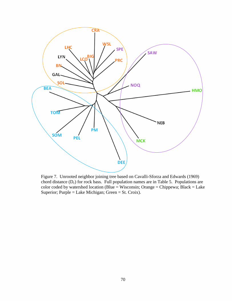
70

Figure 7. Unrooted neighbor joining tree based on Cavalli-Sforza and Edwards (1969)

chord distance (Dc) for rock bass. Full population names are in Table 5. Populations are

color coded by watershed location (Blue = Wisconsin; Orange = Chippewa; Black = Lake

Superior; Purple = Lake Michigan; Green = St. Croix).

71

Figure 8. Unrooted neighbor joining tree based on Cavalli-Sforza and Edwards (1969)

chord distance (Dc) for johnny darters. Full population names are in Table 7.

Populations are color coded by watershed location (Blue = Wisconsin; Orange =

Chippewa; Black = Lake Superior; Purple = Lake Michigan; Green = St. Croix).

72

Figure 9. Mantel test comparing pairwise Dest values versus FST (θ) values for rock bass.

y = 0.6326x - 0.0331

R² = 0.7832

p = 0.001

0.00

0.05

0.10

0.15

0.20

0.25

0.30

0.35

0.40

0.45

0.00 0.10 0.20 0.30 0.40 0.50 0.60

Des

t

FST (θ)

73

Figure 10. Mantel test comparing pairwise Dest values versus FST (θ) values for johnny

darters.

y = 1.6001x - 0.0061

R² = 0.8527

p = 0.001

0.00

0.10

0.20

0.30

0.40

0.50

0.60

0.70

0.80

0.90

0.00 0.10 0.20 0.30 0.40 0.50

Des

t

FST (θ)

74

Figure 11. Results from STRUCTURE v2.3.3 following the modified Coulon et al. (2008) method of assignment for rock bass.

Dashed boxes represent unreconciled groups and solid boxes represent stable groupings at K=1. Populations with (+) indicate most

likely group but failed to assign with >75% probability and are assumed to be individual units.

Full Data Set

22 Populations n=1092

Group 1

TOM HMO

PM MCK BEA PEL

SOM DEE

NOQ+

Group 2

SAW WSL

SPE LYN BIG CRA

BN GAL

PRC LHC LCO + NAB

SOL+

Subgroup 1a

TOM PM

BEA PEL

SOM DEE

Subgroup 1b

HMO MCK

Subgroup 2a

BIG CRA BN GAL

PRC LHC

LCO WSL

LYN

Subgroup 2b SPE SAW

Subgroup 1a1

TOM+ PM PEL

Subgroup 2b1 SPE

Subgroup 2b

SAW

Subgroup 1b1

HMO

Subgroup 1b2 MCK

Subgroup 1a2

BEA SOM

Subgroup 1a3

DEE

Subgroup 1a11

PM

Subgroup 1a12

PEL

Subgroup 1a12

BEA

Subgroup 1a12

SOM

75

Figure 12. Results from STRUCTURE v2.3.3 following the modified Coulon et al. (2008) method of assignment for johnny

darters. Dashed boxes represent unreconciled groups and solid boxes represent stable groupings at K=1. Populations with (+)

indicate most likely group but failed to assign with >75% probability and are assumed to be individual units.

Full Data Set

16 Populations

n=784

Group 4

MC

BUT

Subgroup 1a

TOM

PM

Subgroup

6b

HMO

Subgroup 6a

NAB

MCK

Subgroup 4a

MC

Subgroup 4b

BUT

Subgroup 1a1

TOM

Subgroup 6a2

MCK

Group 1

TOM

PM

BEA Group 5

BIG

WSL

BN

PRC+ Group 6

NAB

MCK

HMO

Group 3

SOL Group 2

LCO

Group 7

NOQ

Group 8

LYN

Subgroup

1b

BEA

Subgroup 5a

BIG

Subgroup 5b

WSL

Subgroup 5c

BN

Subgroup 1a2

PM

Subgroup 6a1

NAB

76

Figure 13. Mantel test comparing geographic distance (km) and genetic differentiation

(Dest) between all populations of sampled rock bass.

y = 0.0004x + 0.0574

R² = 0.1262

p = 0.01

0.00

0.05

0.10

0.15

0.20

0.25

0.30

0.35

0.40

0.45

0 50 100 150 200 250 300 350 400

Gen

etic

Dif

fere

nti

ati

on

(D

est)

Geographic Distance (km)

77

Figure 14. Mantel test comparing geographic distance (km) and genetic differentiation

(Dest) between all populations sampled for johnny darters.

y = 0.0007x + 0.2437

R² = 0.1445

p = 0.01

0.00

0.10

0.20

0.30

0.40

0.50

0.60

0.70

0.80

0.90

0 50 100 150 200 250 300 350 400

Gen

etic

Dif

fere

nti

ati

on

(D

est)

Geographic Distance (km)

78

(a)

(b)

Figure 15. (a) Nine resolved genetic units for rock bass. All sub-watersheds are color

coded to match units in which they grouped. (b) Composite map of walleye and

muskellunge genetic units as described in Figure 2 and 3.

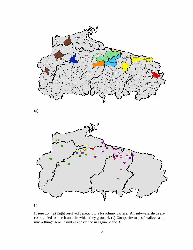
79

(a)

(b)

Figure 16. (a) Eight resolved genetic units for johnny darters. All sub-watersheds are

color coded to match units in which they grouped. (b) Composite map of walleye and

muskellunge genetic units as described in Figure 2 and 3.