Genetic Drift - Rice Universitynakhleh/COMP571/Slides-Fall2010/GeneticDrift.pdfand Inbreeding So...
59
Genetic Drift COMP 571 - Fall 2010 Luay Nakhleh, Rice University
Transcript of Genetic Drift - Rice Universitynakhleh/COMP571/Slides-Fall2010/GeneticDrift.pdfand Inbreeding So...

Genetic DriftCOMP 571 - Fall 2010
Luay Nakhleh, Rice University

Outline
(1) The effects of sampling
(2) Models of genetic drift
(3) Effective population size
(4) Drift and inbreeding
(5) The coalescent model

(1) The Effects of Sampling
One of the assumption of HW is that population size is very large, effectively infinite
However, all biological populations, without exception, are finite
How does the population size affect allele and genotype frequencies?
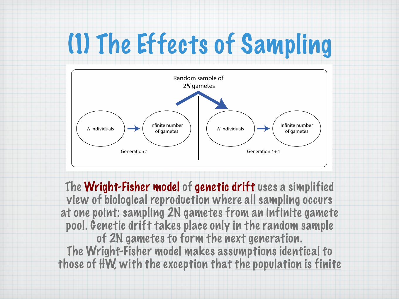
(1) The Effects of Sampling
The Wright-Fisher model of genetic drift uses a simplifiedview of biological reproduction where all sampling occurs
at one point: sampling 2N gametes from an infinite gametepool. Genetic drift takes place only in the random sample
of 2N gametes to form the next generation.The Wright-Fisher model makes assumptions identical to
those of HW, with the exception that the population is finite
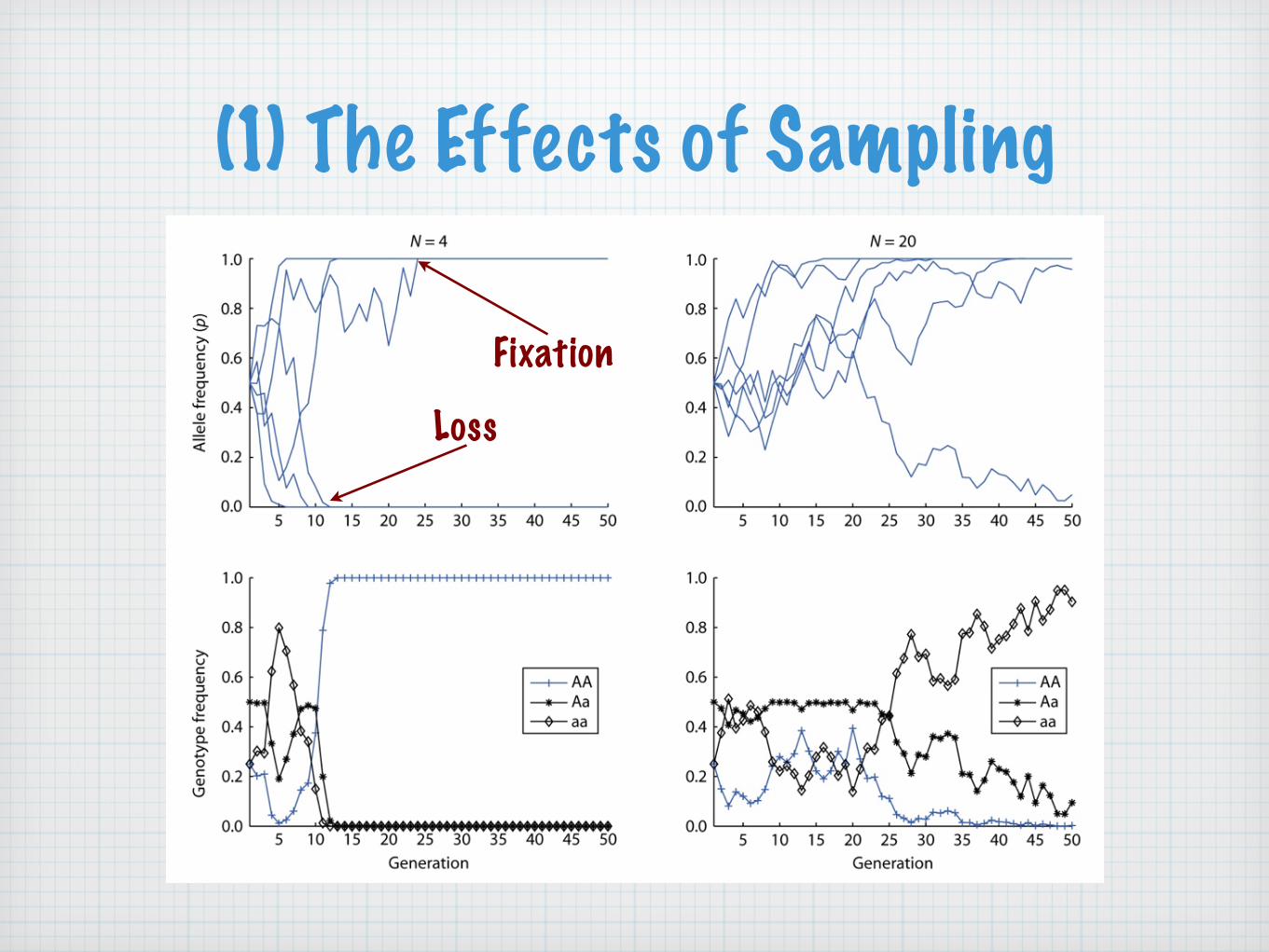
(1) The Effects of Sampling
Fixation
Loss

(1) The Effects of Sampling

(1) The Effects of SamplingUnder the Wright-Fisher model:
the direction of changes in allele frequency is random
the magnitude of random fluctuations in allele frequencies from generation to generation increases as the population size decreases
fixation or loss is the equilibrium state
genetic drift changes allele frequencies and thereby genotype frequencies
the probability of eventual fixation of an allele is equal to its initial frequency
(2) Models of Genetic Drift
Three probability models can be used to illustrate properties of the process of genetic drift:
the binomial probability distribution
Markov chains
diffusion approximation (we will not cover it)

(2) Models of Genetic Drift
Assuming a single locus with alleles A and a at frequencies p and q at a certain generation t (p+q=1)
If 2N gametes are drawn at random to produce the zygotes of the next generation (t+1), the probability that the sample contains exactly i alleles of type A is the binomial probability
The Binomial Probability Distribution
�2N
i
�piq2N−i =
(2N)!i!(2N − i)!
piq2N−i

(2) Models of Genetic DriftThe Binomial Probability Distribution
2N=4 2N=20p=q=0.5

(2) Models of Genetic Drift
The variance of a binomial random variable is σ2=pq
The Binomial Probability Distribution
2N=20
dark blue: allele frequency = 0.5while: allele frequency = 0.75
light blue: allele frequency = 0.95

(2) Models of Genetic DriftThe Binomial Probability Distribution
N=10
The standard deviation and standard error are, respectively:
σ =√
pq SE =�
pq
2N

(2) Models of Genetic DriftThe Binomial Probability Distribution
Genetic drift is less effective at spreading out the distribution of allele frequencies as alleles approach
fixation or loss
(2) Models of Genetic Drift
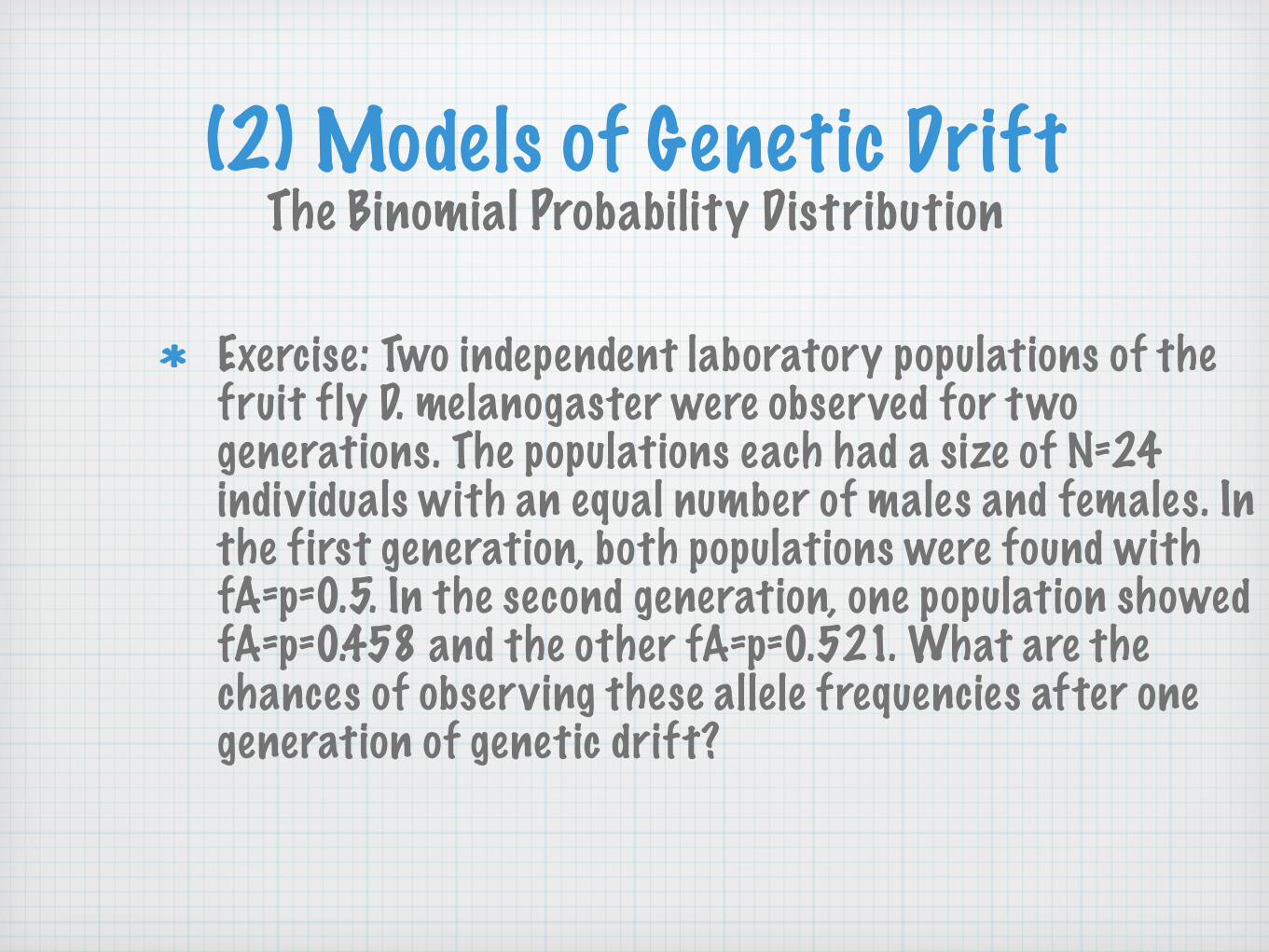
Exercise: Two independent laboratory populations of the fruit fly D. melanogaster were observed for two generations. The populations each had a size of N=24 individuals with an equal number of males and females. In the first generation, both populations were found with fA=p=0.5. In the second generation, one population showed fA=p=0.458 and the other fA=p=0.521. What are the chances of observing these allele frequencies after one generation of genetic drift?
The Binomial Probability Distribution
(2) Models of Genetic Drift
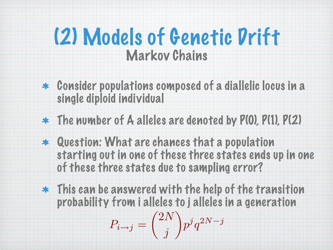
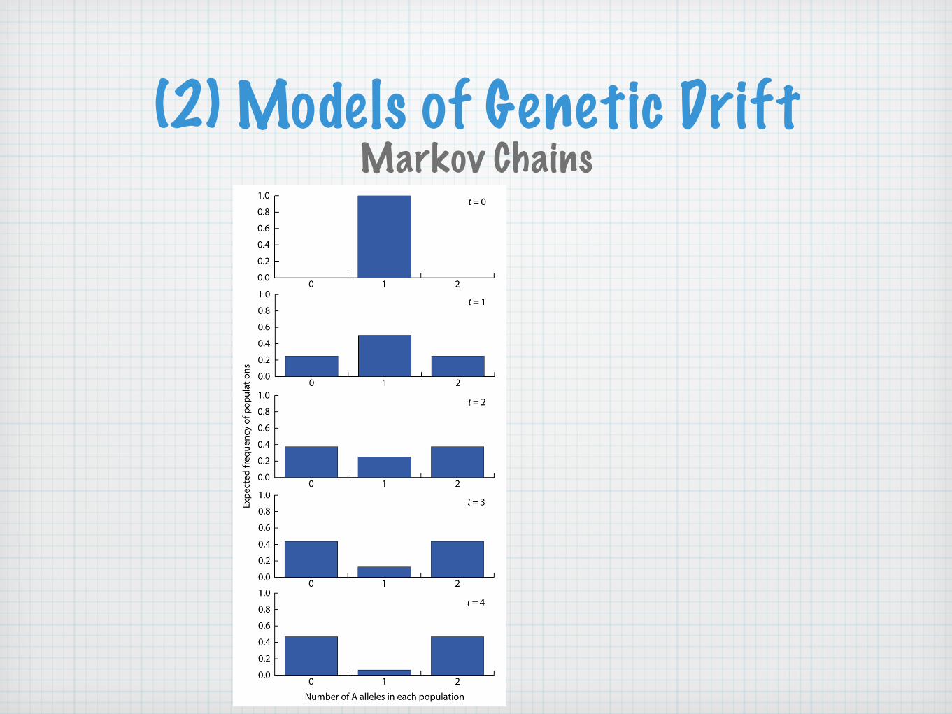
Consider populations composed of a diallelic locus in a single diploid individual
The number of A alleles are denoted by P(0), P(1), P(2)
Question: What are chances that a population starting out in one of these three states ends up in one of these three states due to sampling error?
This can be answered with the help of the transition probability from i alleles to j alleles in a generation
Markov Chains
Pi→j =�
2N
j
�pjq2N−j
(2) Models of Genetic DriftMarkov Chains
One generation later (t=1)
One generation later (t=1)
One generation later (t=1) Initial state: # of A alleles (t=0)Initial state: # of A alleles (t=0)Initial state: # of A alleles (t=0)Initial state: # of A alleles (t=0)Initial state: # of A alleles (t=0)
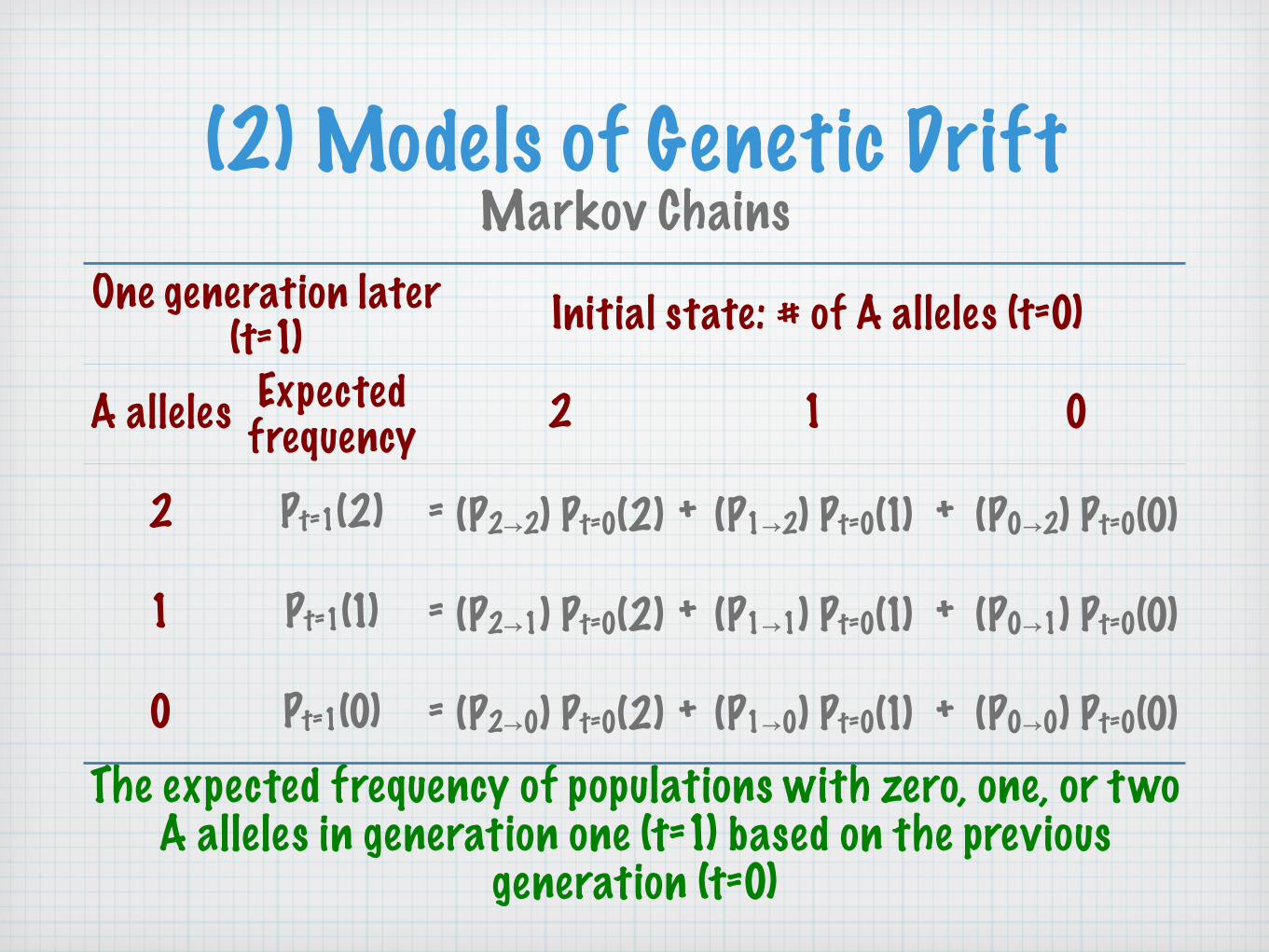
A alleles Expected frequency 2 1 0
2 Pt=1(2) = (P2→2) Pt=0(2) + (P1→2) Pt=0(1) + (P0→2) Pt=0(0)
1 Pt=1(1) = (P2→1) Pt=0(2) + (P1→1) Pt=0(1) + (P0→1) Pt=0(0)
0 Pt=1(0) = (P2→0) Pt=0(2) + (P1→0) Pt=0(1) + (P0→0) Pt=0(0)The expected frequency of populations with zero, one, or two
A alleles in generation one (t=1) based on the previous generation (t=0)

(2) Models of Genetic DriftMarkov Chains
One generation later (t=1)
One generation later (t=1)
One generation later (t=1) Initial state: # of A alleles (t=0)Initial state: # of A alleles (t=0)Initial state: # of A alleles (t=0)Initial state: # of A alleles (t=0)Initial state: # of A alleles (t=0)
A alleles Expected frequency 2 1 0
2 Pt=1(2) = (P2→2) Pt=0(2) + (P1→2) Pt=0(1) + (P0→2) Pt=0(0)
1 Pt=1(1) = (P2→1) Pt=0(2) + (P1→1) Pt=0(1) + (P0→1) Pt=0(0)
0 Pt=1(0) = (P2→0) Pt=0(2) + (P1→0) Pt=0(1) + (P0→0) Pt=0(0)
0
0
0
0
1
1
The expected frequency of populations with zero, one, or twoA alleles in generation one (t=1) based on the previous
generation (t=0)
(2) Models of Genetic DriftMarkov Chains
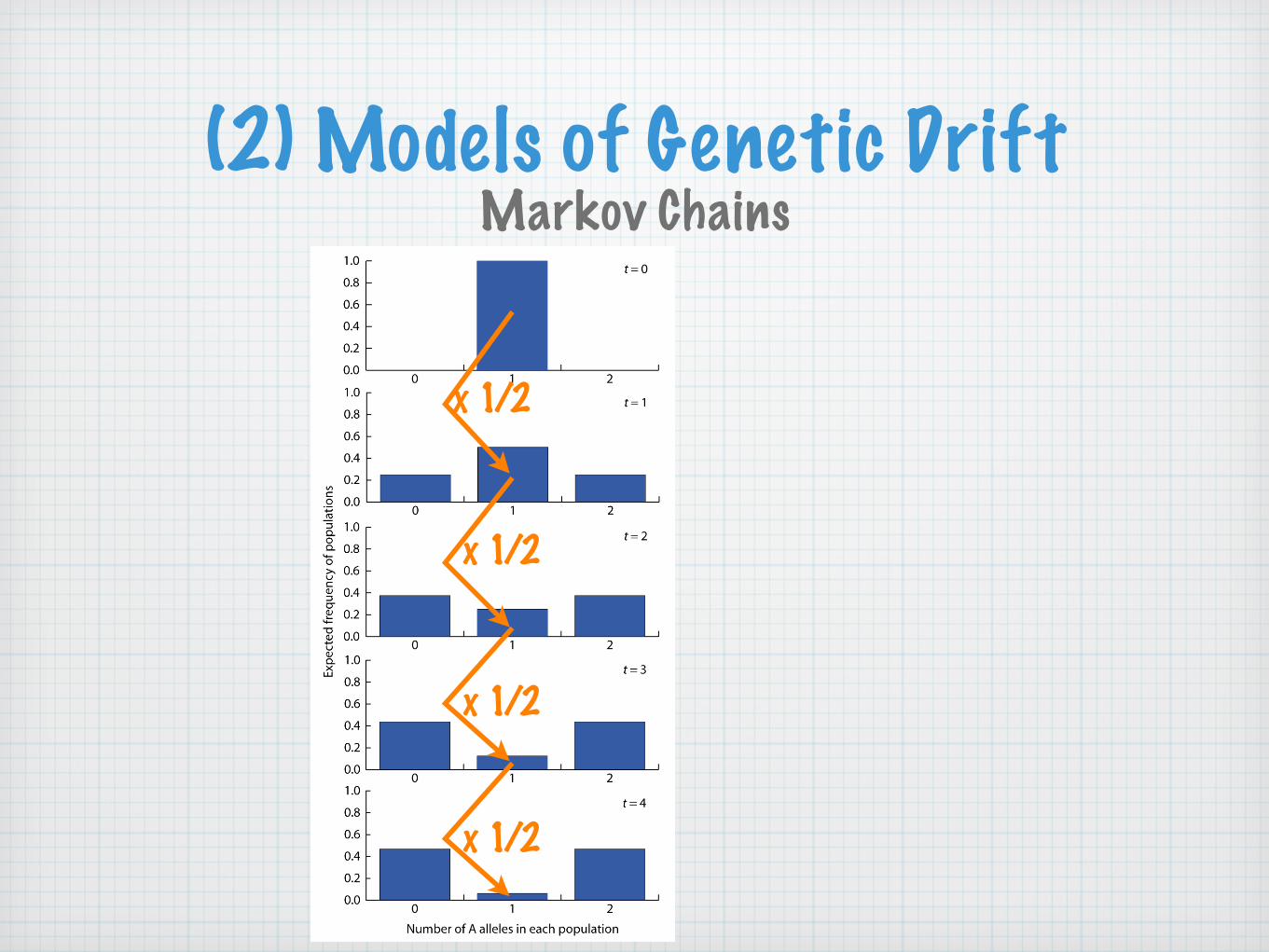
(2) Models of Genetic DriftMarkov Chains
x 1/2
x 1/2
x 1/2
x 1/2
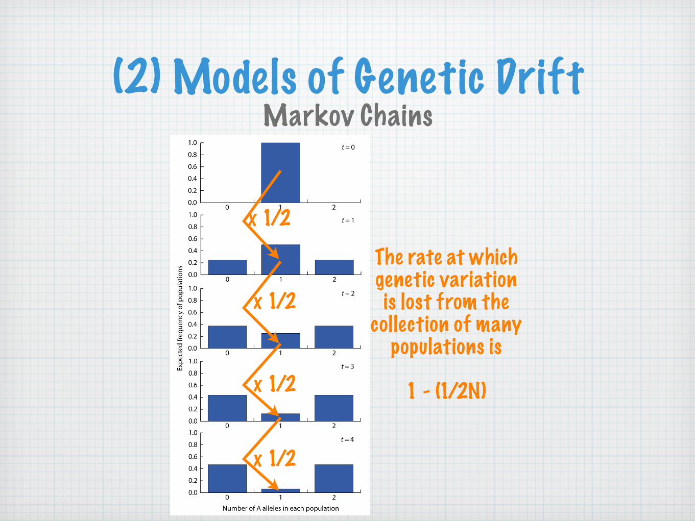
(2) Models of Genetic DriftMarkov Chains
x 1/2
x 1/2
x 1/2
x 1/2
The rate at whichgenetic variationis lost from the
collection of manypopulations is
1 - (1/2N)
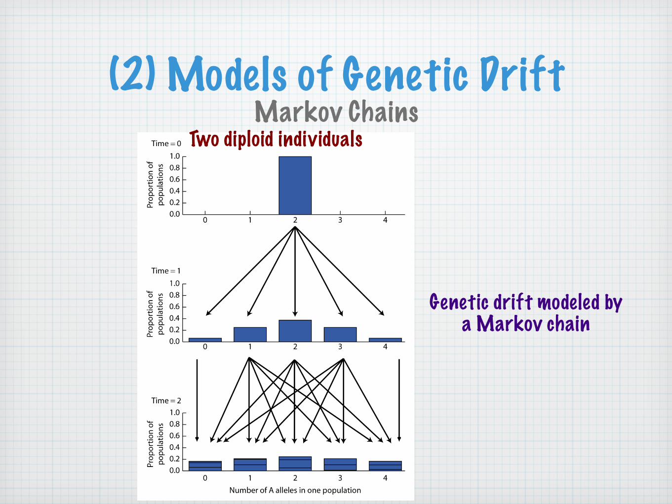
(2) Models of Genetic DriftMarkov Chains
Two diploid individuals
Genetic drift modeled by a Markov chain
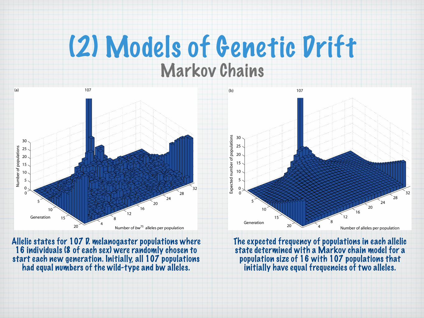
(2) Models of Genetic DriftMarkov Chains
Allelic states for 107 D. melanogaster populations where16 individuals (8 of each sex) were randomly chosen to
start each new generation. Initially, all 107 populationshad equal numbers of the wild-type and bw alleles.
The expected frequency of populations in each allelicstate determined with a Markov chain model for a
population size of 16 with 107 populations that initially have equal frequencies of two alleles.

(2) Models of Genetic Drift
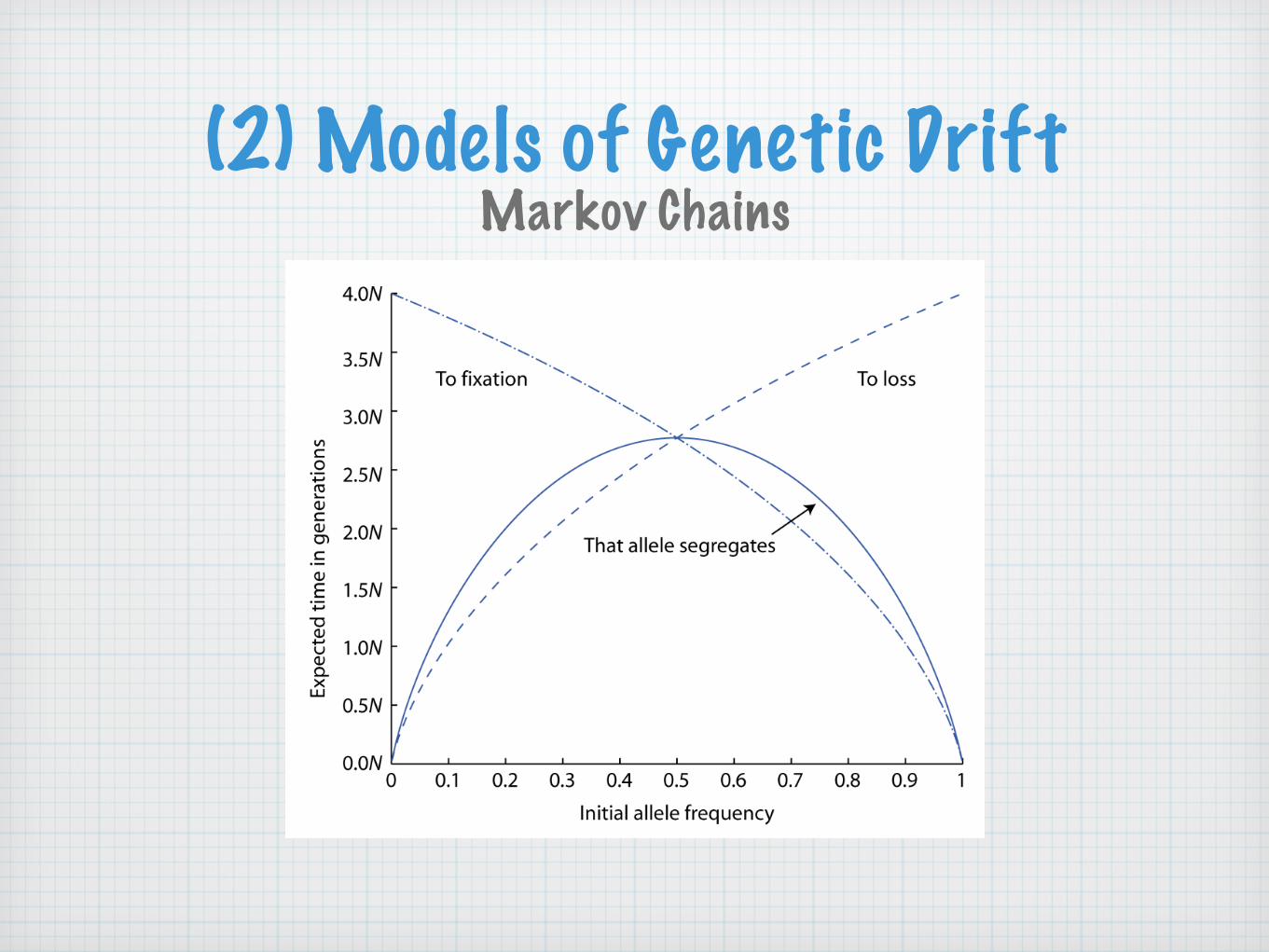
The average time to fixation for alleles that eventually fix in a population and the average time to loss for alleles that eventually are lost from a population are, respectively:
Markov Chains
T fix = −4N(1− p) ln(1− p)
pT loss = −4N
p ln p
1− p
where p is the initial allele frequency.
The mean persistence time of an allele is:
T segregate = pT fix + (1− p)T loss = −4N [(1− p) ln(1− p) + p ln p]
(2) Models of Genetic DriftMarkov Chains

(3) Effective Population Size
In most biological populations it is difficult, or impossible, to determine the number of gametes that contribute to the next generation
Therefore, we need to define the size of populations in a way that’s different from “the number of individuals in a population”
The definition of the population size in population genetics relies on the dynamics of genetic variation in the population (i.e., the size of a population is defined by the way genetic variation in the population behaves)
(3) Effective Population Size
Census population size (N): the number of individuals in a population
Effective population size (Ne): the size of an ideal Wright-Fisher population that maintains as much genetic variation or experiences as much genetic drift as an actual population regardless of census size

(3) Effective Population Size
Cases where a population may deviate from the ideal of the Wright-Fisher model:
Fluctuating population size
Breeding sex ratio
Variation in family size
Subdivided population
(3) Effective Population Size
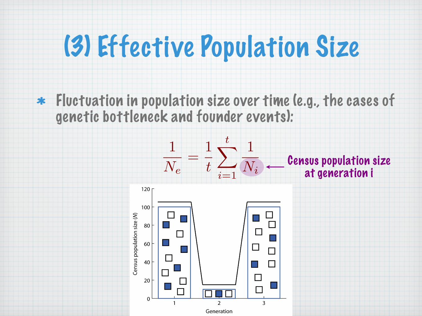
Fluctuation in population size over time (e.g., the cases of genetic bottleneck and founder events):
1Ne
=1t
t�
i=1
1Ni
Census population sizeat generation i

(3) Effective Population Size
When Nm and Nf are the numbers of females and males, respectively, breeding in the population, and all other assumptions of Wright-Fisher populations are met, we have:
Ne = 4NmNf
Nm + Nf
if Nm=1 or Nf=1
Ne≈4
if Nm=Nf=N/2
Ne≈N

(3) Effective Population SizeWhen there is variation in family size, where Nt-1 is the size of the parental population and k is the number of gametes that result in progeny, we have:
Ne =4Nt−1
var(k) + k2 − k

(3) Effective Population Size
When the population is divided into d demes, each of size N, and migration between demes occurs at rate m, we have:
Ne = N +(d− 1)2
4md

(4) Parallelism Between Drift and Inbreeding
So far: genetic drift and population size
We now demonstrate that finite population size can be thought of as a form of inbreeding
Genetic drift occurs due to finite population size
As populations get smaller, the probability of inbreeding increases
Therefore, genetic drift and the tendency for inbreeding are interrelated phenomena, connected to the size of the population
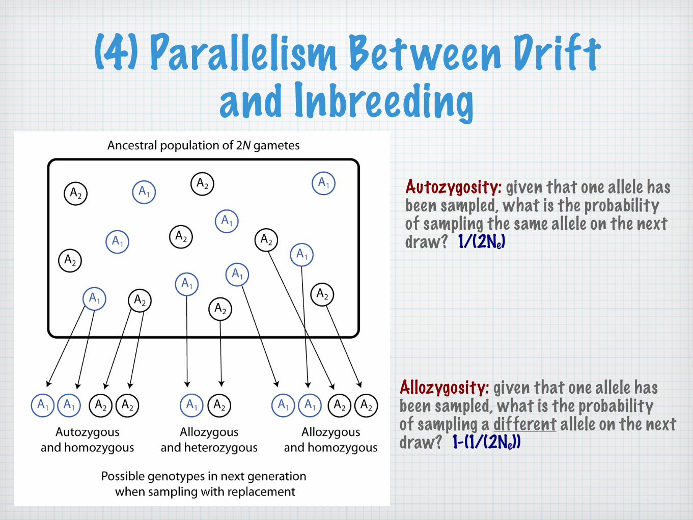
(4) Parallelism Between Drift and Inbreeding
Autozygosity: given that one allele has been sampled, what is the probability of sampling the same allele on the next draw? 1/(2Ne)
Allozygosity: given that one allele has been sampled, what is the probability of sampling a different allele on the next draw? 1-(1/(2Ne))

(4) Parallelism Between Drift and Inbreeding
We can use the probability of autozygosity in a finite population to define the fixation index as
Ft =1
2Ne
for generation t under the assumption that none of thealleles in the gamete pool in generation t-1 are identicalby descentTo make it more general, we have
Ft =1
2Ne+
�1− 1
2Ne
�Ft−1
sampling betweengenerations
the proportion of apparentlyallozygous alleles that are actually
autozygous due to past sampling or inbreeding
(4) Parallelism Between Drift and Inbreeding
By definition, F is the reduction in heterozygosity as well as the increase in homozygosity compared to HW expected frequencies
If F is proportional to the homozygosity and amount of inbreeding, then 1-F is proportional to the amount of heterozygosity and random mating

(4) Parallelism Between Drift and Inbreeding
Ft =1
2Ne+
�1− 1
2Ne
�Ft−1
1− Ft =�
1− 12Ne
�(1− Ft−1)
Eq. 2.20: Ht=2pq(1-Ft)Ht
2pq=
�1− 1
2Ne
� �Ht−1
2pq
�
Ht =�
1− 12Ne
�Ht−1 Ht =
�1− 1
2Ne
�t
H0
initial heterozygosity
heterozygosity aftert generations
Ht ≈ H0e−t/2N
(4) Parallelism Between Drift and Inbreeding
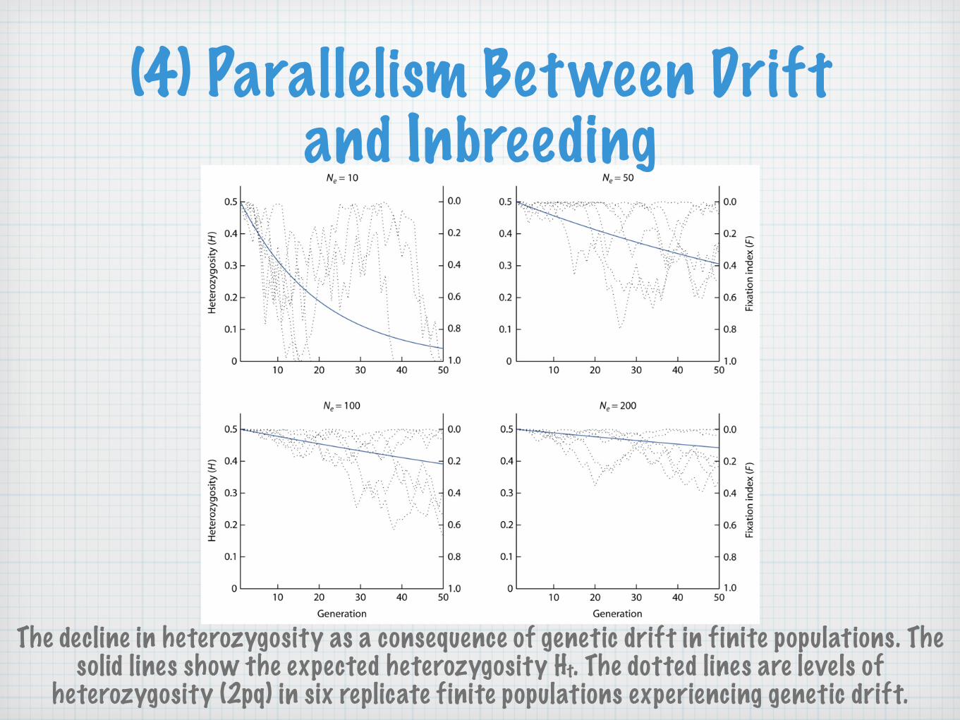
The decline in heterozygosity as a consequence of genetic drift in finite populations. The solid lines show the expected heterozygosity Ht. The dotted lines are levels of
heterozygosity (2pq) in six replicate finite populations experiencing genetic drift.
(4) Parallelism Between Drift and Inbreeding
Conclusions:
Genetic drift causes populations to become more inbred in the sense that autozygosity and homozygosity increase even though mating is random
Mating systems where there is consanguineous mating cause genetic variation in populations to behave as if the effective population size were smaller than it would be under complete random mating

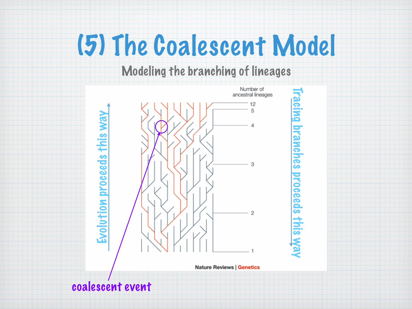
(5) The Coalescent ModelModeling the branching of lineages
Evolu
tion
proc
eeds
this
way
Tracing branches proceeds this way
(5) The Coalescent ModelModeling the branching of lineages
Evolu
tion
proc
eeds
this
way
Tracing branches proceeds this way
coalescent event

(5) The Coalescent ModelModeling the branching of lineages
Evolu
tion
proc
eeds
this
way
Tracing branches proceeds this way
coalescent event most recent common ancestor(MRCA)
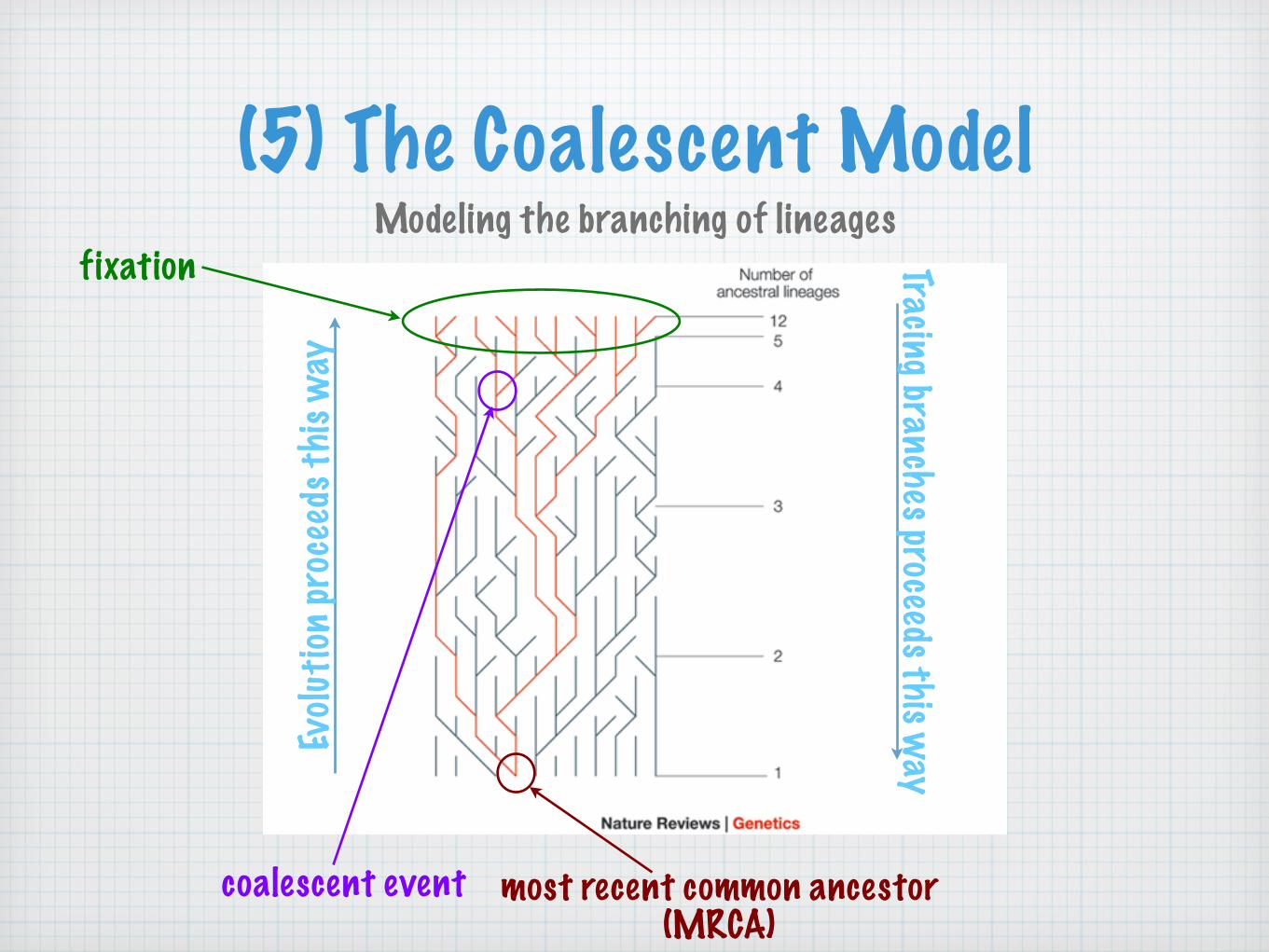
(5) The Coalescent ModelModeling the branching of lineages
Evolu
tion
proc
eeds
this
way
Tracing branches proceeds this way
coalescent event most recent common ancestor(MRCA)
fixation
(5) The Coalescent ModelModeling the branching of lineages
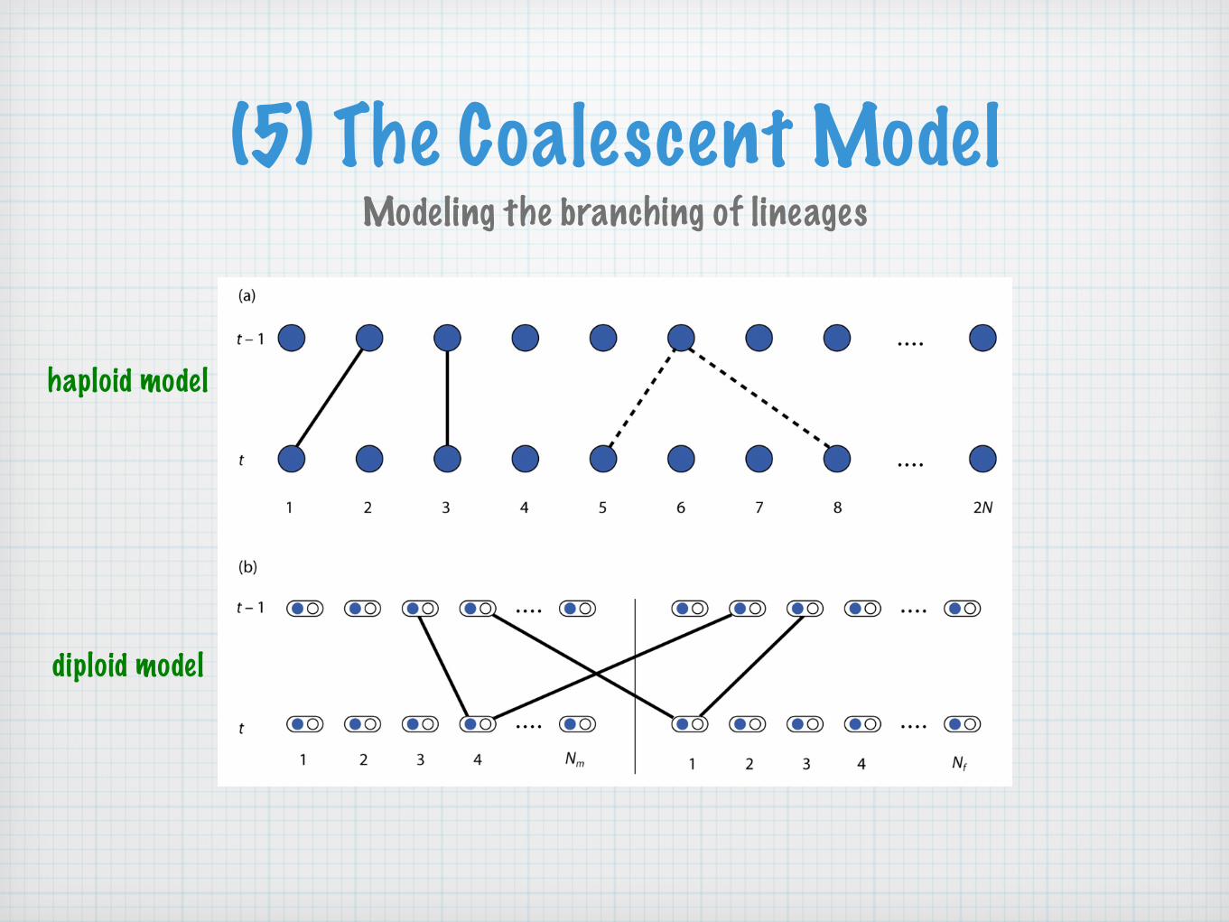
haploid model
diploid model

(5) The Coalescent ModelModeling the branching of lineages
probability = 1/2N
haploid model
diploid model
(5) The Coalescent ModelModeling the branching of lineages
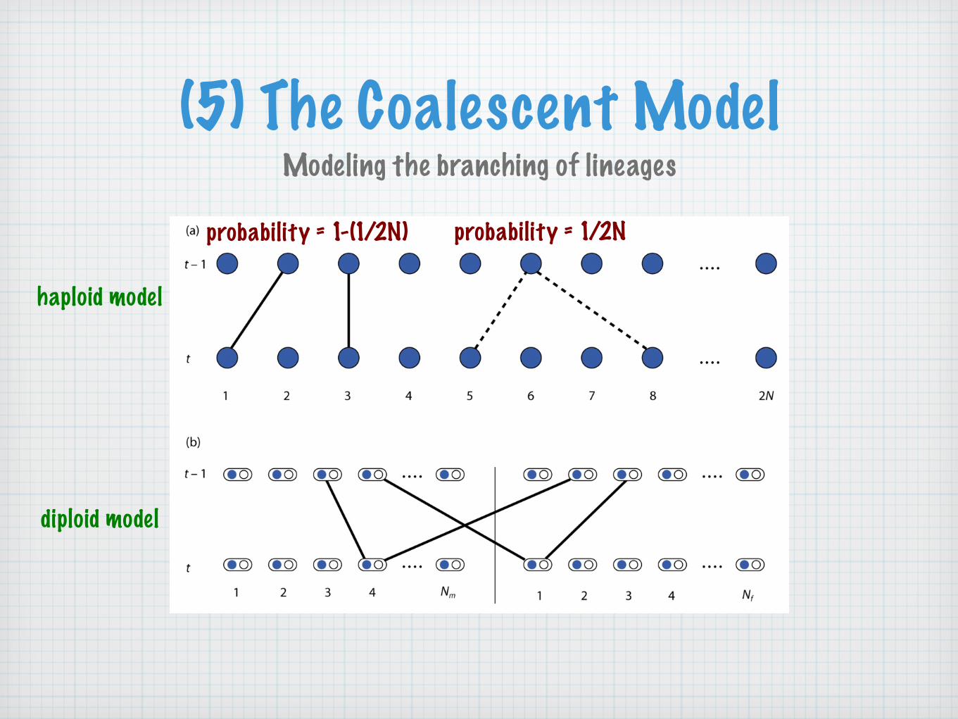
probability = 1/2Nprobability = 1-(1/2N)
haploid model
diploid model

(5) The Coalescent ModelModeling the branching of lineages
probability = 1/2Nprobability = 1-(1/2N)
haploid model
diploid model
The haploid model with 2N lineages is routinely used to approximate the diploid model with N=Nf+Nm diploid individuals

(5) The Coalescent ModelModeling the branching of lineages
The probability that two randomly chosen lineagescoalesce after exactly t generations is
�1− 1
2N
�t−1 12N
The cumulative probability that two randomly chosen lineagescoalesce at or before generation t is approximated by the
exponential distribution
P (TC ≤ t) = 1− e−1
2N t

(5) The Coalescent ModelModeling the branching of lineages

(5) The Coalescent ModelModeling the branching of lineages
Recall that for exponential distribution, we have:
It follows that the average time to coalescence and the variance in time to coalescence are, respectively
pdf : λe−λx cdf : 1− e−λx µ :1λ
σ2 :1λ2
11
2N
= 2N and1
�1
2N
�2 = 4N2

(5) The Coalescent ModelModeling the branching of lineages
Recall that for exponential distribution, we have:
It follows that the average time to coalescence and the variance in time to coalescence are, respectively
pdf : λe−λx cdf : 1− e−λx µ :1λ
σ2 :1λ2
11
2N
= 2N and1
�1
2N
�2 = 4N2
⇒ the length of branches connecting lineages to their ancestors will be highly variable around their mean values

(5) The Coalescent ModelModeling the branching of lineages
(5) The Coalescent ModelModeling the branching of lineages
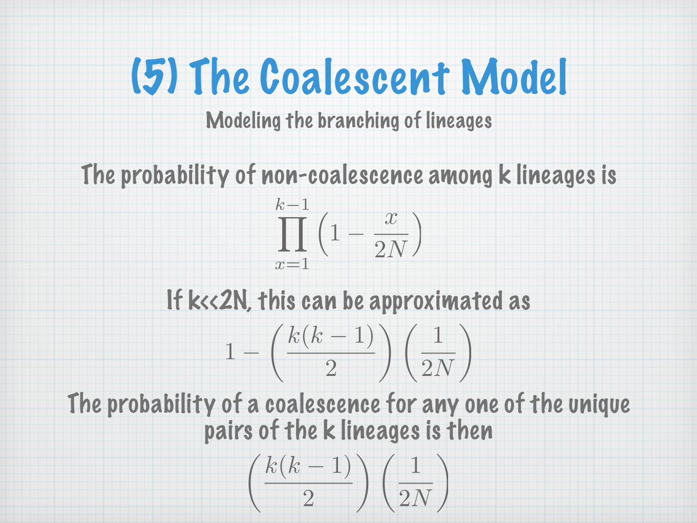
The probability of non-coalescence among k lineages isk−1�
x=1
�1− x
2N
�
If k<<2N, this can be approximated as
1−�
k(k − 1)2
� �1
2N
�
The probability of a coalescence for any one of the unique pairs of the k lineages is then�
k(k − 1)2
� �1
2N
�
(5) The Coalescent ModelModeling the branching of lineages
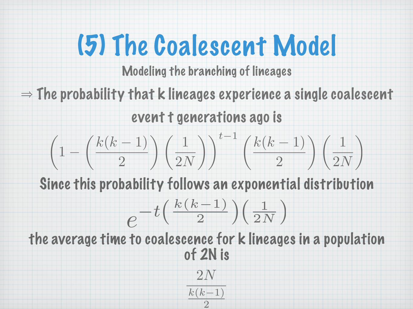
⇒ The probability that k lineages experience a single coalescentevent t generations ago is
�1−
�k(k − 1)
2
� �1
2N
��t−1 �k(k − 1)
2
� �1
2N
�
Since this probability follows an exponential distribution
e−t( k(k−1)2 )( 1
2N )the average time to coalescence for k lineages in a population
of 2N is2N
k(k−1)2
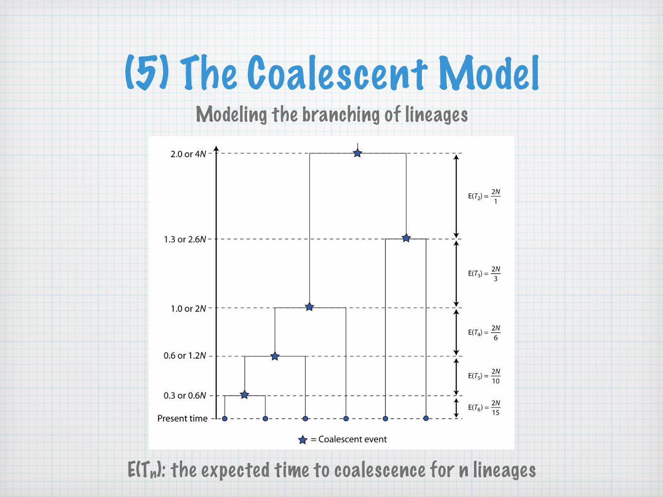
(5) The Coalescent ModelModeling the branching of lineages
E(Tn): the expected time to coalescence for n lineages

(5) The Coalescent ModelModeling the branching of lineages
E(Ti) =2
i(i− 1) V ar(Ti) =�
2i(i− 1)
�2
TMRCA = E(Hk) =k�
i=2
E(Ti) = 2k�
i=2
1i(i− 1)
= 2�
1− 1k
�
Ttotal =k�
i=2
iE(Ti) = 2k�
i=2
i
i(i− 1)= 2
k−1�
i=1
1i
V ar(TMRCA) = 4k�
i=2
1i2(i− 1)2
V ar(Ttotal) = 4k−1�
i=1
1i2

(5) The Coalescent ModelModeling the branching of lineages
The distribution of TMRCA for 1000 replicate genealogies starting with six lineages. Ne=1000.

(5) The Coalescent ModelThe gn,k(t) function
gn,k(t) =
1−�n
i=2e−(i
2)t(2i−1)(−1)in[i]
n(i)if k = 1
�ni=k
e−(i
2)t(2i−1)(−1)i−kk(i−1)n[i]
i!(i−k)!n(i)if k ≥ 2
gn,k(t): the probability that n lineages coalesce into k lineageswithin time t (i.e., that n-k coalescent events occur before
time t in the past
n[i] = n(n− 1) · · · (n− i + 1)n(i) = n(n + 1) · · · (n + i− 1)

SummaryIn finite populations, allele frequencies can change from generation to generation since the sample of gametes that found the next generation may not contain exactly the same number of each allele as the previous generation.
Sampling error in allele frequency causes genetic drift, the random process whereby all alleles eventually reach fixation or loss.
The Wright-Fisher model makes assumptions identical to HW in addition to assuming that each generation is founded by a sample of 2N gametes from an infinite pool of gametes.
The action of genetic drift can be modeled by the binomial distribution, a Markov chain model, and the diffusion approximation.

SummaryThe effective population size (Ne) is the size of an ideal Wright-Fisher population that shows the same frequency behavior over time as an observed biological population regardless of its census population.
Finite population size and consanguineous mating are analogous processes, since they both lead to increasing homozygosity and decreasing heterozygosity. The distinction is that genetic drift in finite populations causes changes in both genotype and allele frequencies while consanguineous mating changes only genotype frequencies.
The coalescent models the branching of lineages to predict the time to the MRCA.