Genetic Algorithms - Stony Brook Universitybender.astro.sunysb.edu/.../lectures/genetic.pdfGenetic...
31
PHY 604: Computaonal Methods in Physics and Astrophysics II Genec Algorithms
Transcript of Genetic Algorithms - Stony Brook Universitybender.astro.sunysb.edu/.../lectures/genetic.pdfGenetic...
PHY 604: Computational Methods in Physics and Astrophysics II
Genetic Algorithms
PHY 604: Computational Methods in Physics and Astrophysics II
Genetic Algorithms
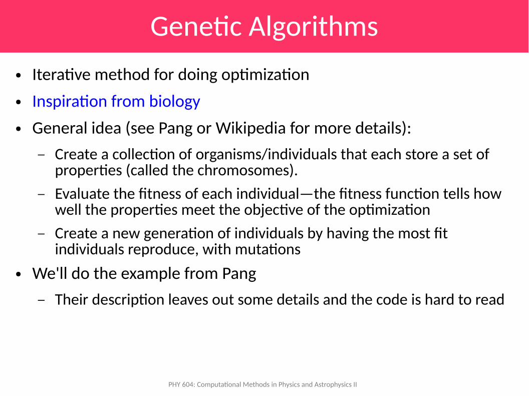
● Iterative method for doing optimization
● Inspiration from biology
● General idea (see Pang or Wikipedia for more details):
– Create a collection of organisms/individuals that each store a set of properties (called the chromosomes).
– Evaluate the fitness of each individual—the fitness function tells how well the properties meet the objective of the optimization
– Create a new generation of individuals by having the most fit individuals reproduce, with mutations
● We'll do the example from Pang
– Their description leaves out some details and the code is hard to read
PHY 604: Computational Methods in Physics and Astrophysics II
Model Problem: Thomson Problem
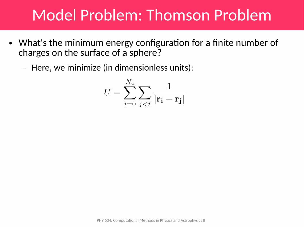
● What's the minimum energy configuration for a finite number of charges on the surface of a sphere?
– Here, we minimize (in dimensionless units):
PHY 604: Computational Methods in Physics and Astrophysics II
Model Problem: Thomson Problem
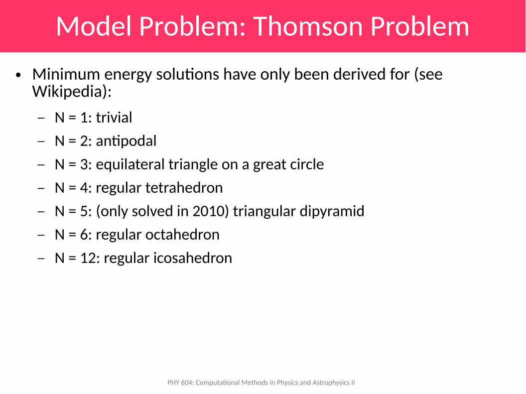
● Minimum energy solutions have only been derived for (see Wikipedia):
– N = 1: trivial
– N = 2: antipodal
– N = 3: equilateral triangle on a great circle
– N = 4: regular tetrahedron
– N = 5: (only solved in 2010) triangular dipyramid
– N = 6: regular octahedron
– N = 12: regular icosahedron
PHY 604: Computational Methods in Physics and Astrophysics II
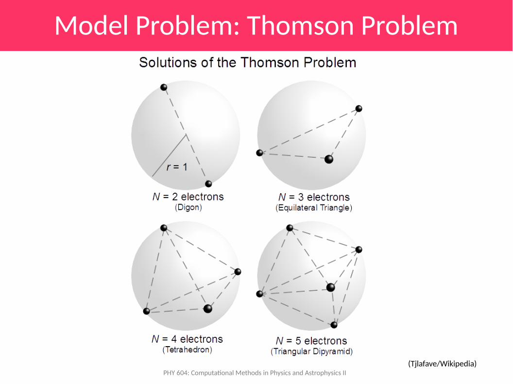
Model Problem: Thomson Problem
(Tjlafave/Wikipedia)
PHY 604: Computational Methods in Physics and Astrophysics II
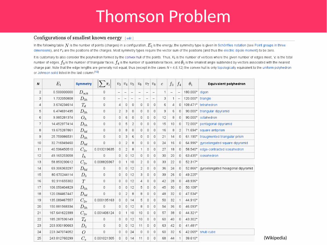
Thomson Problem
(Wikipedia)
PHY 604: Computational Methods in Physics and Astrophysics II
Binary Algorithm
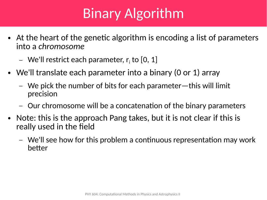
● At the heart of the genetic algorithm is encoding a list of parameters into a chromosome
– We'll restrict each parameter, ri to [0, 1]
● We'll translate each parameter into a binary (0 or 1) array
– We pick the number of bits for each parameter—this will limit precision
– Our chromosome will be a concatenation of the binary parameters
● Note: this is the approach Pang takes, but it is not clear if this is really used in the field
– We'll see how for this problem a continuous representation may work better
PHY 604: Computational Methods in Physics and Astrophysics II
Binary Algorithm
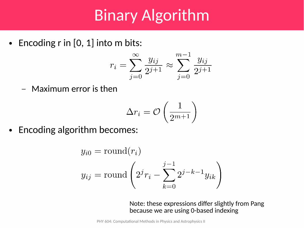
● Encoding r in [0, 1] into m bits:
– Maximum error is then
● Encoding algorithm becomes:
Note: these expressions differ slightly from Pang because we are using 0-based indexing
PHY 604: Computational Methods in Physics and Astrophysics II
Encoding and Decoding
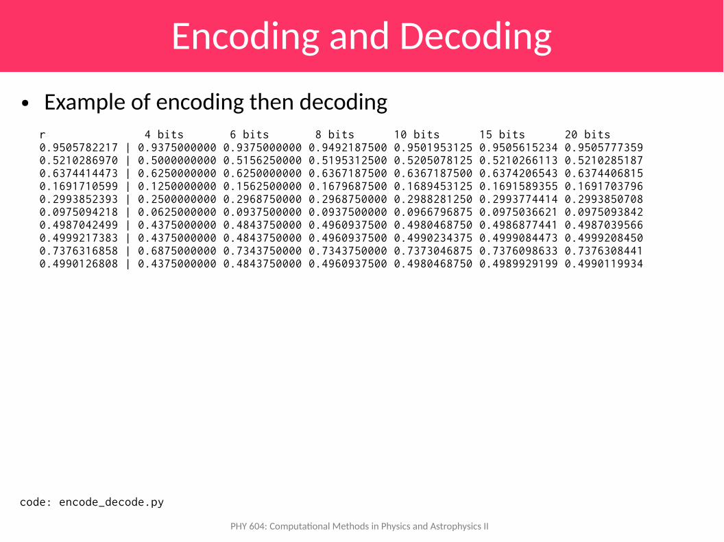
● Example of encoding then decodingr 4 bits 6 bits 8 bits 10 bits 15 bits 20 bits 0.9505782217 | 0.9375000000 0.9375000000 0.9492187500 0.9501953125 0.9505615234 0.9505777359 0.5210286970 | 0.5000000000 0.5156250000 0.5195312500 0.5205078125 0.5210266113 0.5210285187 0.6374414473 | 0.6250000000 0.6250000000 0.6367187500 0.6367187500 0.6374206543 0.6374406815 0.1691710599 | 0.1250000000 0.1562500000 0.1679687500 0.1689453125 0.1691589355 0.1691703796 0.2993852393 | 0.2500000000 0.2968750000 0.2968750000 0.2988281250 0.2993774414 0.2993850708 0.0975094218 | 0.0625000000 0.0937500000 0.0937500000 0.0966796875 0.0975036621 0.0975093842 0.4987042499 | 0.4375000000 0.4843750000 0.4960937500 0.4980468750 0.4986877441 0.4987039566 0.4999217383 | 0.4375000000 0.4843750000 0.4960937500 0.4990234375 0.4999084473 0.4999208450 0.7376316858 | 0.6875000000 0.7343750000 0.7343750000 0.7373046875 0.7376098633 0.7376308441 0.4990126808 | 0.4375000000 0.4843750000 0.4960937500 0.4980468750 0.4989929199 0.4990119934
code: encode_decode.py
PHY 604: Computational Methods in Physics and Astrophysics II
Encoding and Decoding
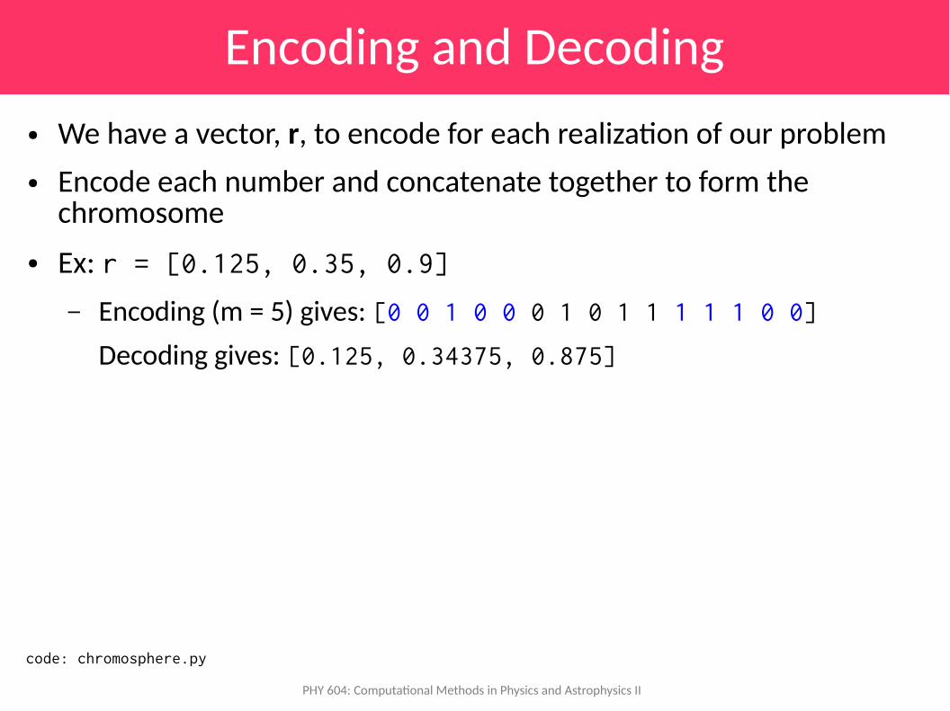
● We have a vector, r, to encode for each realization of our problem
● Encode each number and concatenate together to form the chromosome
● Ex: r = [0.125, 0.35, 0.9]
– Encoding (m = 5) gives: [0 0 1 0 0 0 1 0 1 1 1 1 1 0 0]
Decoding gives: [0.125, 0.34375, 0.875]
code: chromosphere.py
PHY 604: Computational Methods in Physics and Astrophysics II
Encoding and Decoding
● Sometimes your parameters might already be integers, in which case the encoding and decoding step is trivial and you can operate on the binary representation of the data
PHY 604: Computational Methods in Physics and Astrophysics II
Overview of GA
● Create a population
– N different realizations: creatures, organisms, phenotypes
– Randomly pick parameters and encode into a chromosome
● Select parents
– The fittest of the population should “breed” and create the next generation
● Crossover
– Swap genes between the parent chromosomes to create the children
● Mutation
– Randomly change some bits to introduce new data into the population
PHY 604: Computational Methods in Physics and Astrophysics II
Cost / Fitness Function
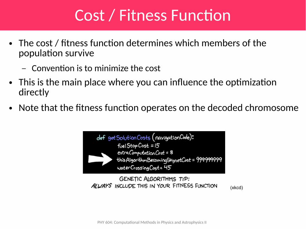
● The cost / fitness function determines which members of the population survive
– Convention is to minimize the cost
● This is the main place where you can influence the optimization directly
● Note that the fitness function operates on the decoded chromosome
(xkcd)
PHY 604: Computational Methods in Physics and Astrophysics II
Initialization
● We want a population of N creatures
– For the Thomson problem, each creature needs 2 parameters for each charge
● spherical angles theta, phi
● Some variation: create 2N and keep the N fittest
– We'll need a sorting method → order according to cost function
● Create the initial parameters for each creature via a random number generator (restricted to [0, 1))
– Encode these to form the initial chromosome
PHY 604: Computational Methods in Physics and Astrophysics II
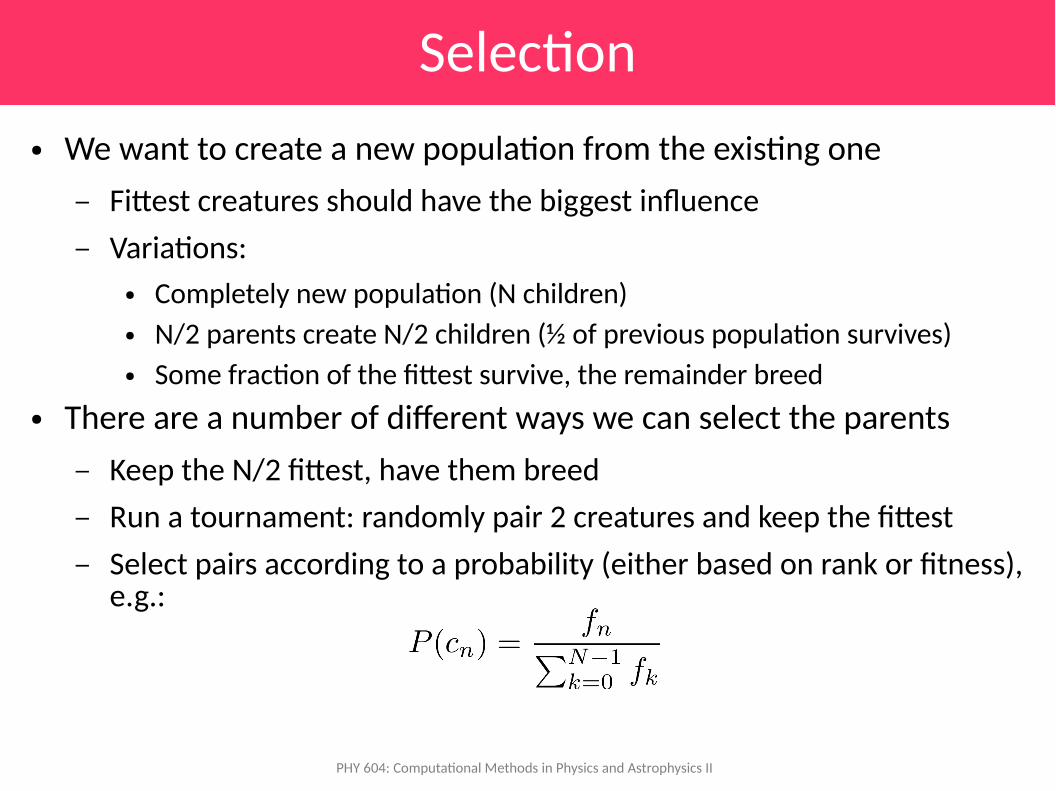
Selection
● We want to create a new population from the existing one
– Fittest creatures should have the biggest influence
– Variations:
● Completely new population (N children)● N/2 parents create N/2 children (½ of previous population survives)● Some fraction of the fittest survive, the remainder breed
● There are a number of different ways we can select the parents
– Keep the N/2 fittest, have them breed
– Run a tournament: randomly pair 2 creatures and keep the fittest
– Select pairs according to a probability (either based on rank or fitness), e.g.:
PHY 604: Computational Methods in Physics and Astrophysics II
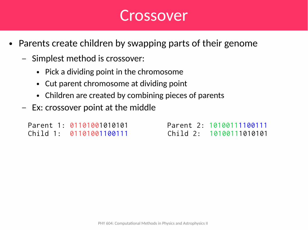
Crossover
● Parents create children by swapping parts of their genome
– Simplest method is crossover:
● Pick a dividing point in the chromosome● Cut parent chromosome at dividing point● Children are created by combining pieces of parents
– Ex: crossover point at the middle
Parent 1: 01101001010101 Parent 2: 10100111100111Child 1: 01101001100111 Child 2: 10100111010101
PHY 604: Computational Methods in Physics and Astrophysics II
Mutation
● Your crossover may never introduce new values of parameters, if you cut the chromosome right at a boundary of parameters
● Mutation can introduce more genetic diversity (just like in nature)
● This is an essential part of the algorithm
● Some variations:
– Mutate before or after crossover?
– Keep the best (elite) creatures unmutated?
● Basic parameters:
– Pick a mutation percentage
– Flip bits in the chromosome based on the probability of mutation
PHY 604: Computational Methods in Physics and Astrophysics II
Overall algorithm
● Basic flow:
– Create the initial population
– Do Ng generations:
● Select parents● Perform crossover● Do mutation
PHY 604: Computational Methods in Physics and Astrophysics II
Thomson Problem
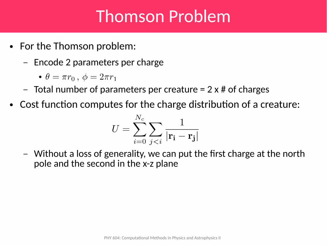
● For the Thomson problem:
– Encode 2 parameters per charge
●
– Total number of parameters per creature = 2 x # of charges
● Cost function computes for the charge distribution of a creature:
– Without a loss of generality, we can put the first charge at the north pole and the second in the x-z plane
PHY 604: Computational Methods in Physics and Astrophysics II
Thomson Problem
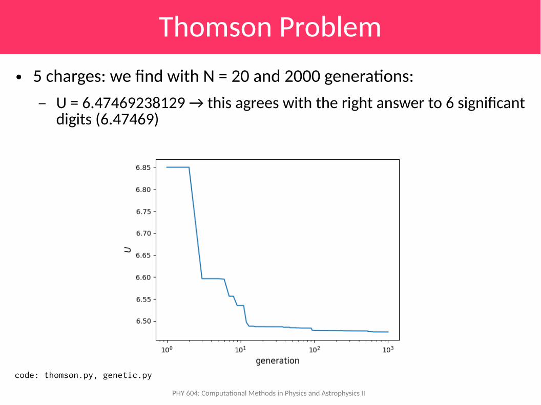
● 5 charges: we find with N = 20 and 2000 generations:
– U = 6.47469238129 → this agrees with the right answer to 6 significant digits (6.47469)
code: thomson.py, genetic.py
PHY 604: Computational Methods in Physics and Astrophysics II
Thomson Problem
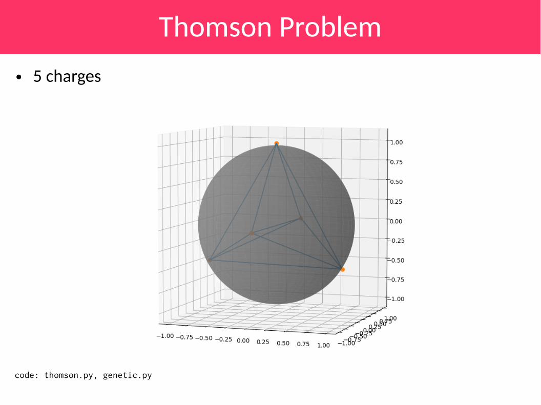
● 5 charges
code: thomson.py, genetic.py
PHY 604: Computational Methods in Physics and Astrophysics II
Thomson Problem
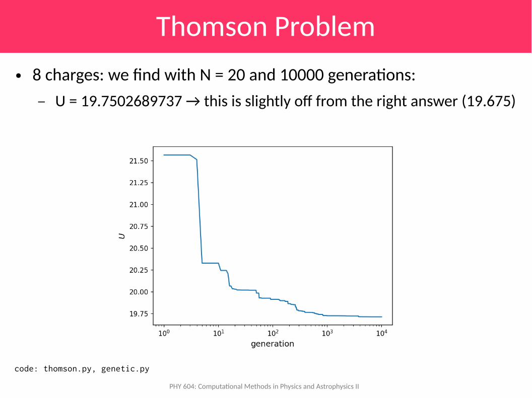
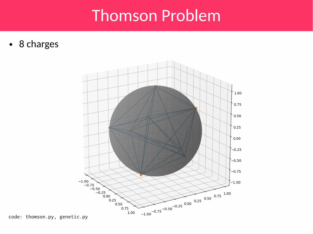
● 8 charges: we find with N = 20 and 10000 generations:
– U = 19.7502689737 → this is slightly off from the right answer (19.675)
code: thomson.py, genetic.py
PHY 604: Computational Methods in Physics and Astrophysics II
Thomson Problem
● 8 charges
code: thomson.py, genetic.py
PHY 604: Computational Methods in Physics and Astrophysics II
Variations
● Mutation rate, population size, … all can affect the performance
● At the core, we have a random process, so running several realizations will show uncertainty
● The code is a little complicated—let's go over it
– We'll view the output interactively so we can rotate it around
PHY 604: Computational Methods in Physics and Astrophysics II
Genetic Cars
● Here's a cool online example: genetic cars
– http://rednuht.org/genetic_cars_2/
● Optimizes the design of a car using a genome consisting of:
– Shape: (8 genes, 1 per vertex)
– Wheel size: (2 genes, 1 per wheel)
– Wheel position: (2 genes, 1 per wheel)
– Wheel density: (2 genes, 1 per wheel) darker wheels mean denser wheels
– Chassis density: (1 gene) darker body means denser chassis
PHY 604: Computational Methods in Physics and Astrophysics II
Continuous Algorithm
● Chromosome is an array of real numbers
– Not converted into a bit representation
● No longer need encode and decode methods
● Selection is largely unchanged, since the cost function operates on the real parameters already
● Crossover:
– Simplest: cut the array at a boundary of elements and swap
● In our binary method, we could conceivably cut a parameter's representation and swap it, resulting in a completely new value of that parameter
– Some methods exist which allow for the real numbers themselves to be changed
PHY 604: Computational Methods in Physics and Astrophysics II
Continuous Algorithm
● Mutation: this can actually change the parameters
– Simplest method: just call a random number generator to change one of the parameters according to the mutation probability
– Note that this introduces a bigger change than flipping a single bit (especially with binary Gray coding)
● Benefits:
– Should be faster, since we avoid all the encoding and decoding
– Has better precision (since double precision numbers use 64 bits instead of the m ~ 20 we were using with the binary algorithm)
PHY 604: Computational Methods in Physics and Astrophysics II
Continuous Algorithm
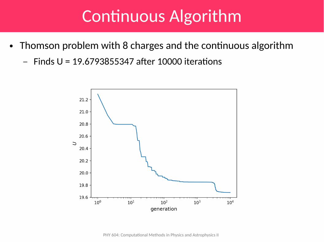
● Thomson problem with 8 charges and the continuous algorithm
– Finds U = 19.6793855347 after 10000 iterations
PHY 604: Computational Methods in Physics and Astrophysics II
Binary vs. Continuous
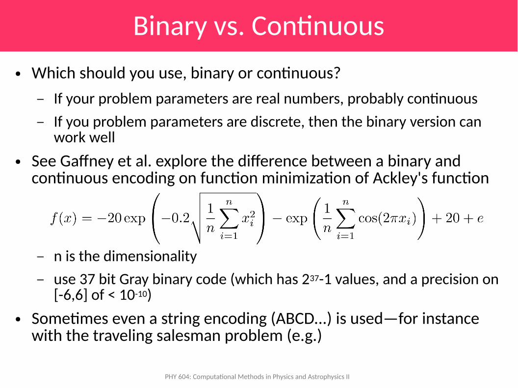
● Which should you use, binary or continuous?
– If your problem parameters are real numbers, probably continuous
– If you problem parameters are discrete, then the binary version can work well
● See Gaffney et al. explore the difference between a binary and continuous encoding on function minimization of Ackley's function
– n is the dimensionality
– use 37 bit Gray binary code (which has 237-1 values, and a precision on [-6,6] of < 10-10)
● Sometimes even a string encoding (ABCD...) is used—for instance with the traveling salesman problem (e.g.)
PHY 604: Computational Methods in Physics and Astrophysics II
Simulated Annealing vs. GA?
● Both simulated annealing and genetic algorithms can be used for optimization problems
– Both have the strength that the random nature helps avoid local minima
– Folklore seems to suggest that simulated annealing is the faster / preferred method
PHY 604: Computational Methods in Physics and Astrophysics II
Simulated Annealing vs. GA?
● Let’s solve the Thomson problem using simulated annealing
● We need a move set:
– Pick a charge at random
– Pick one of the angles and perturb it by a small amount (using a Gaussian normal random number)
– Make sure the angles stay within their bounds
– Accept the move according to the Metropolis probability condition