GENETIC ALGORITHMS APPLIED TO MULTI-OBJECTIVE AERODYNAMIC SHAPE OPTIMIZATION

Terry L. Hoist NASA Ames Research Center

Moffett Field, CA 94035

Abstract

A genetic algorithm approach suitable for solving multi-objective optimization problems is described and ev2!vltPr( nsinl: 2 series e! r~rodynimic s h i p e?!imizatinn ,nmh!ems. Several new features including two variations of a binning selection algorithm and a gene-space transformation procedure are included. The genetic algorithm is suitable for finding pareto optimal solutions in search spaces that are defined by any number of genes and that contain any number of local exlrsma. A new masking array capability is included allowing any gene or gene subset to be eliminated as decision variables from the design space. This allows determination of the effect of a sing!e gene CI gene s ~ b s e t on the pareto optimal solution. Results indicate that the genetic algorithm optimization approach is flexible in application and rsliable. The binning selection algctrithms generally p:ovide paret:, front quality enhancements 2nd moderate convergence efficiency improvements for most of the problems solved.

Nomenclature

set of scalar objective functions optimal set of F values scalar objective function maximum value of f r/n GA generation (active file) integer ranking array seed value used in the random number generator R(0,l) user-specified integer parameter controlling which selection algorithm is used user-specified integer parameter controlling the gene-space transformation option fixed number of chromosomes in each GA generation number of genes in each chromosome number of scalar objective functions user-specified vector with four elements that controls modification operator usage user-specified parameter controlling probability that a specific gene will be modified using perturbation mutation operator (0 I A 5 1) user-specified parameter controlling probability that a specific gene will be modified using giobai mutation operaior (0 2 fi 5 7) basis vector matrix with elements < random number generator that returns a random value between 0 and 1 unitary transformation matrix with elements q,j /' gene from the j" chromosome and the d' GA generation

jh chromosome tiom the f l GA generation

user-specified maximum limit on the I"' gene

user-specified minimum limit on tS!e Gene use;-specifi& paramete: conir=ilir;g tke size =f the pe,<s:bstjc-,r: ,T;ctaticns (0 < 9 5 1)

https://ntrs.nasa.gov/search.jsp?R=20040084446 2019-03-10T10:16:37+00:00Z

..

subscriDts i

k

suDerscriDts

c

i

/I

gene or declsion variabie mdex chromosome index objective function index

GA generation or population index temporary chromosome values obtained after selection but before modification

Backaround

Numerical methods for optimizing the performance of engineering problems have been studied for many years. Perhaps the most widely used general approach involves the computation of sensitivity gradients. These methods-called gradient methods-have been utilized to produce optimal engineering performance in a wide variety ot different forms. The reiiabiiity and success of gradient meihods generaiiy requires a smooth design space and the existence of only a single global extremum or an initial guess close e , ~ ~ g h :O the global ext:emum that will ensure proper convergence.

In contrast to gradient-based methods, design space search methods such as genetic algorithms (GA)-also referred to as evolutionary algorithms (EA)-offer an alternative approach with several attractive features. The basic idea associated with the GA approach is to search for optimal solutions using an analogy to the theory of evolution. The problem to be optimized is parameterized into a set of decision variables or genes. Each set of genes that fully defines one design is called an individual or a chromosome. A set of chromosomes is called a population or a generation. Each complete design or chromosome is evaluated using a “biological-like” fitness function that determines survivability of that particular chromosome. For example, in aerospace applications, the genes may be a series of geometric parameters associated with an aerospace vehicle that is to be optimized for payload delivered to orbit, aerodynamic performance or structural weight. The fitness function takes as input all the geometric parameters and returns a numerical value for the fitness-the size of the payload, the aerodynamic performance or the structural weight.

During solution advance (or “evolution” using GA terminology) each chromosome is ranked according to its fitness vmter-~ne fitness va!ue fer each ebjective. The higher-ranking chromosomes are se!ected to continue to the next generation while the lower-ranking chromosomes are not selected at all. The newly selected chromosomes in the next generation are manipulated using various operators (combination, crossover or mutation) to create the final set of chromosomes for the new generation. These chromosomes are then evaluated for fitness and the process continues-iterating from generation to generation-until a suitable level of convergence is obtained or until a specified number of generations has been completed.

Constraints can easily be included in the GA optimization approach either by direct inclusion into the objective function definition-a so-called penalty constraint-or, more commonly, by including one or more constraints into the fitness function evaluation procedure. For example, if a design violates a constraint, its fitness is set to zero, that is, it does not survive to the next generation. Because GA DptiiiiiiZtiGii is EO: a giadknt-b2s& optimization technique, it dces nct need‘ sensitivity derivati\ves. It theoretically works well in non-smooth design spaces containing several or perhaps many local extrema.

General GA detaiis including descriptions o i basic genetic aigorithm concepts can be iound in Goldberg,’ Davis,’ and Beasley, et al.3’4 Additional useful studies, which survey recent activities in the area of GA research includiiig the presentation of model probiems useful for evaiuating GA per?‘ormance are gives i!? Deb,5 Vs: ?/e!rihnizen 2 n d Lammt6 and Jimknez, et a1.7

2

A disadvantage of the GA approach is expense. lq general, the number of function evaluatims required for a G.4 optimization process io converge, exceeds t h e number of fiinc:ion evaluatl~ns required by a finite-difference-based gradient optimization (see the results presented in Obayashi and Tsukaharag a n a Bock9). This situation is offset, to an extent, by the ease with which GAS can b e implemented in parallel or distributed computing environments.

Despite being relativeiy new, genetic algorithm have already been applied in many applications ovei a broad range of engineering fields. A brief survey of single discipline applications is presented in Holst and Pulliam,'' and will not be discussed further in this report.

Other applications involving GA search methods have been made in t h e area of multi-objective or multi- discipline optimization, that is, optimization problems in which two or more objectives are simultaneously and independently optimized. These methods, referred to as MOGA jmuiii-objective genetic algorithm) methods, are especially attractive because they offer the ability to directly compute so-called "pareto optimal sets" in a single computation instead of the limited single design point traditionally provided by other methods.

The pareto optimal s e t oi pareto front, as it is comrnor;ly called, includes optimal solutions for each of t h e individual objectives, as well as a range of tradeoff solutions in between, which are themselves optimal solutions. Providing a range of solutions to a multi-objective optimization problem is a powerful approach because it allows the designer to see the effect of decision variable variation on the design space in t h e form of optimal tradeoffs. Thus, the designer can choose individual objective weighting factors after their L . . ! ! L L ! .-.._- ' -'.n.-.t'+n+f.:.-.!:: !..F..T:a,5 IUII t i i itLeii~e is c(ua1ItttattvGty RIIWIUII.

ii7 iecogni i i~n Gf the iii;poeai;ze of the MOGA apprcach, many theoretical developrnents have bee!! published in recent years. In particular, Van Veldhuizen and Lamont' and Zitzler, et al." present reasonably complete surveys of MOGA methodofogy with a special emphasis on how to compare GA performance from o n e algorithm variation to another. Other researchers, including Deb,' Deb, e t al.," Van V e l d h ~ i z e n , ' ~ Lohn, e t al.ld and Holst and Pulliarn,'' have developed and/or utilize a suite of tes t problems as a standard in evaluating MOGA convergence efficiency as well as the accuracy of the final pareto front. A key aspect of pareto front development is diversity. Does a particular MOGA produce good coverage over the entire pareto front or are some regions poorly resolved while other regions have high levels of undesirable clustering? This issue is studied in Laumanns, e t a1.16 and Deb, et al."

Still other MOGA issues are associated with archive strategies. As t h e pareto front develops, many solutions a r e found that lie on the pareto front that cannot be retained within the fixed population size of many schemes . How to retain or archive this information for the benefit of the MOGA while maintaining reasonable bounds on t h e archive file h a s been studied in Knowles and C r ~ n e . ' ~ ~ ' ~ O n e last example of MOGA research lies in the area of an interactive algorithm development. P a r n e e , e t al?' present a MOGA approach that allows changes to b e made in GA operators as well as in objective definitions as the MOGA advances from generation to generation.

One area of MOGA research that is even more voluminous than the area of theoretical developments is that associated with dA multi-objective applications. Examples of multi-objective optimization applications include airfoil optimization by Marco, et al.," Naujoks, et a1.,22 Quagliarelia and Delia C i ~ p p a , ' ~ Vicini and Q~agliarella, '~ Hamalainen, et al." 2nd Epstein and missile aeroaynarnic'shape optimization by Anderson, et ai.," and wing optimization by Anderson and Gebert," Sasaki, e t al.,B Oyama,30 Obayashi, et al.,31 and Ng, et aI.=

Additional MOGA examples in the area of turbomachinery optimization include rocket engine turbopump design by Cyam2 and L i c ~ ~ ~ and compressor blade design by Benni34 and Oyama and L ~ o u . ~ ~ In s o m e of these examples the multiple objectives were obtained by considering two different aerodynamic design

3

points. In others the multiple objectives involved different disciplines including aerodynamics, structures, controls and/or electromagnetics. One iast area of GA research that beais ri-iefitiofi is in the area of hybiid methods, the u!i!izs?ion of CP. optimization in conjunction with another type of optimizer. This is an attractive area of research because GA methods are particularly good at finding a global extrema, but not particularly good in converging the optimal solution to tight levels of accuracy. Briefly, several examples where hybrid approaches have been utilized include Rap and M a d a ~ a n ~ ~ for single objective problems and Giotis, et aI.,% Tursi,% Vicini and Quagliarelia” and Brown and Smiin4’ for multi-objective probiems.

Various definitions and the multi-objective genetic algorithm used in the present study are described next. Details associated with each of the operators, including selection, passthrough, random average crossover, perturbation mutation and mutation are presented. MOGA effectiveness is then evaluated using several three-dimensional aerodynamic shape optimization problems.

Problem Statement: Sinclle Obiective Optimization

A single-objective optimization problem can be stated as fcllows: Let f be a scalar function of NG independent variab!es, x,, defined ny! some domain 0 I

!R this notation X is the vector of design space decision variables. The maximum value of f ! indicated by f , is obtained by finding the values of X = X’ such thatt

The above maximization operation is subject to Nco conditions or constraints indicated by

The constraints placed on the decision variabie vector X by Eqs. (IC) essentially servs to firnit the design space within Q for which the optimal solution is sought.

Problem Stat emen t : Mu it i-0 biec t ive 0 Dt i m iza t io n

For Optimization problems involving more than one objective, which are simultaneously and independently optimized, the situation is more difficult. This is because each objective must play a role in determining the optimal solution. In the optimization process, conflicts might arise among the various objzctive functicns, that is, the +tima! vil!ues o! each individm! objective, in genera!, will not occur for the same decision variable vector, X . As a result, the “optimal solution” for a multi-objective optimization

i

, problem is typically a range or a set of solutions, which represent tradeoffs in objective space.

To determine when one solution is better than another for mu!ti-objective optimization problems the concept of dominance is utilized.‘ A vector ti =U(r/,,...,u,,-..,u,) is said io dominaie another vector V = V( v,,. ., vi,. . ., v,,,) if and only if L$ 2 5 for all i and there exists at least one value of i such that uj > y;. A vector defined on some domain Q that is not dominated by any other vector defined on Qis said to be non-dominated on Q .

For the purpose of simplifying the discussion of algorithmic details, maximization is generally assumed The logic for minirnizaticn is a strzightforward modiiicetion and will not be discussed.

A multi-objective optimization problem can be stated as follows: Let F be a set of No scalar objective functions, 4 , each dependent upon the same decision variable vector, X , which is defined on some design space Q

As above, :he decision variable vector X consists of NG independen? components. The multi-objective optimization problem involves finding the set of X = X * that produces non-dominated values for F = F* on Q . This set of values F* is called the pareto optimal s e t or the pareto front.

For each F the constraints

C"(X)SO n= 1,2;.-,/yC0 (2b j

must be satisfied. Existence of these constraints serves to limit or reduce the size of L2 for which the optimal solution is sought.

Genetic Alaorithrn

The genetic algorithm optimization procedure utilized to solve the multi-objective optimization problem, as described by Eqs. (2), is now presented. It is closely related to the MOGA optimization procedure presented in Holst and Pulliam." As mentioned in the iniroauciion, the generai idea behind Gk optimization is to discretely describe the design space using a number of decision variables, xi. In GA parlance these parameters are called genes, and the i subscript refers to the gene number. Each set of genes that leads to the complete specification of an individual design, that is, each decision variable vector, X , is called a chromcsome and is indicated by

where the j subscript, added to X , identifies the chromosome number. In addition, the j' subscript has been added to each gene, to indicate its chromosome membership. The n superscript has been added to indicate the GA generation number, which is iteratively advanced as the solution converges. Thus, Xg is

the 1" chromosome for the nth generation that consists of NG genes.

For aerodynamic shape optimization problems, the design space genes are typically a series of geometric parameters, for example, airfoil thickness and camber and/or wing sweep, twist and taper. For many GA applications genes are computationally represented using bit strings and the operators used to manipulate them are designed to accommodate bit string data. In the present approach, following the aigtiinents of Ojsma," Houck, et ai." and Michaiewjcz," rea!-nurnber encoding is used to represent ail genes.

The key reason for using real number encoding is that it has been shown to be more efficient in terms of CPU time relative to binary encoded GAS.& Ir: addition, real numbers are used for dl genes in the present implementation because the present engineering application involves decision variabies ihai are best described using real numbers, for example, the geometric parameters in aerodynamic shape optimization. Thus, using real number encoding eliminates the need for binary-to-real number conversions.

5

Initialization I

Once the deskjiil space h2.a besn defined ii7 :e;n;s of a set of real-number genes, the next step is tc form an initial generation, G‘, represented by

GO = (X?,. . .,Xo,.-.,Xo 1 NC) (4) where N, is the total number of chromosomes. Each gene within each chromosome is assigned an initial numerical value using a process that randomly chooses numbers between fixed user-specified limits. For example, the th gene in an arbitrary chromosome is initialized using

xj = f lO , l ) ( xmax i - Xmin, ) + Xmin, (5)

where xmax, and xmin, are the upper and lower limits for the iih gene, respectively, and R(0,I) is a random

number generator that delivers an arbitrary numerical value between 0.0 and 1 .O.

The random number generator used in the present study requires an integer input-a seed value. If the integer is positive, the next number in the current random number sequence is returned. tf the integer is negative, t he iandoiii niiriibei sequence is reset to a new sequence. Utilization of the same negative seed value will always reset the random number generator to the same random sequence. Each new solution begins by resetting the random number generator using asingle call to R(0,l) with a negative seed value-ISEED. All other calls to @0,1) during that solution use a positive seed value. Thus, a so!utinn can be repeated by simp!y using the same inltia! seed va!m or rerun to determine statistical variation by using a different initial seed value.

Fitness evaluation

After a generation is established-either the initial generation or any succeeding generation in tne evolutionary process-fitness values, F,?, are computed for each chromosome using a suitable function

evaluation. This is analogous to the objective function evaluation in gradient methods and is represented using

F,? = F(XY) (6) -

For example, for a multi-discipline optimization (MDO) problem involving the simultaneous maximization of two separate and distinct objectives, 4 and 4 , the fitness evaluation represented by Eq. (6) consists of the following

Jn = 4(X,”)

g = h v : ) where, for example, the first function 4 might be the aerodynamic drag of an aerospace vehicle (constrained to fly at fixed lift) and the second function 4 might be the structural mass of the same vehicle. Once all the genes in a specific chromosome have been specified, ,( can be evaluated using a suitable CFD solver to obtain the drag and 4 can be evaluated using a suitable structural analysis routine to obtain the structural mass. In this case, of course, the optimization problem would be one of minimization.

6

Ranking

T I he purpose ~ r i the ranking operation is to d&iKine a set G? integer values for the rankin.; arr~y, L f f . Qne integer value is required ?or each chromosome. The ranking algorithm is quiie different for muiti-objective optimization problems relative to single-objective problems. As such, both situations will be discussed in this section. The ranking array values-once determined-are then used in the GA selection process.

-. Sinaie Obiective Optimization- I ne GA ranking aigorithm for single objective opiimiiaiioil pi&leii;S is quite simple. Whichever chromosome has the highest fitness is ranked number one (/R= l), whichever has the second highest fitness is ranked number two (/R=2), and so on. This ranking algorithm, more formally stated, is given by

(7) 1 ic= 1

/Y(+g)k= ;c+1 j=l , - . . ,N , f = l , . . . , N , /? = /c

-

where j ana )are special counters that range over all N, chromosomes in the current populztion or generation level.

Multi-Objective Optimization-For multi-objective optimization problems the ranking procedure is more complex and utilizes the concept of dominance, which was defined previously.

A chromosome with a fitness vector F that is not dominated by any other fitness vector within the design space is said to be a non-dominated chromosome. The optimal solution set F' or pareto front includes all solutions with fitness vectors that are non-dominated and that satisfy the constraints given by Eqs. (2b). The numerical approximation to the pareto front must involve a suitably complete set of discrete solutions SG as to describe the. c~ptimal values of each individual ebjecti\!+-these are the pareto front endpoints-as well as the non-dominated tradeoff solutions in between the optimal values associated with each of the individual objectives.

With the concept of dominance in hand the actual ranking process can now be presented. There are a number of ranking piocedures available for use in multi-objective optimization. The one used in the present study is called Goldberg ranking.' After all of the fitness values have been determined, each chiDiiiDSGii;S is checked for dominance. Thcse ch:cmoscmes tha! are non-dominated s o niven a number one ranking ( / R = l ) and then temporarily removed from the current generation. The remaining chromosomes that are non-dominated are given a number two ranking (/R= 2) and then temporarily removed. This process continues until each chromosome has an integer value for the ranking array, /R. In general, with this approach, the number of different integer values contained within the ranking array will be small, at least small in comparison to N,, as many chromosomes will be ranked near the top with a value of 1,2 or 3.

Y

The above procedure, by itself, represents a legitimate algorithm for the ranking operation. However, there is a refinement that provides a considerable enhancement to MOGA convergence. Before describing this refinement, two additional concepts must be defined-the active file and the accumulation file.

The active file is simply a specific name used for the current generation of chromosomes, that is

7

is the nth generation active file for the GA iteration process. As the GA solution evolves, the active file is always fixed in size at N, chromosomes. The first No elements in the active file-for the present impiemeniaiion-aiways coniain the chromosomes that posses the maximum fitness v a h s for each of the No objectives.

The accumulation file is the list of all non-dominated chromosomes that have been found from all generations combined during the current MOGA iteration. As the MOGA solution evolves, the accumulation file typically grows in size with more chromosomes being added after each new generation. As new non-dominated chromosomes are added to the accumulation file, old chromosomes that lose their dominance must be deleted, thus ensuring that the accumulation file contains nothing but number-one ranked chromosomes. Because each chromosome stored in the nth generation accumulation file is non-

front. The use of an accumulation file makes sense only when Ncl 2 2. r(nm;nqtnr( it cnntcic tn rlnfino thn nirntn frnnt n r I t lnact tho . ~ t h ~ P n P ~ q t j ~ n 3,DprcYimatiQfl " " I 1 1 1 1 I U L L " " ) I. O V I "VU L V ""'I'IV ' . I - p.-'-.- . ' W I I L Y . , L.. .e--., -..- the pa.reto

i

The multi-objective ranking procedure described above utilizes only the chromosomes in the active file, that is, each chromosome in the active file is ranked relative to the other chromosomes in the active file. But this philosophy potentially wastes a plethora of information because not every number-one ranked chromosome for multi-objective optimization problems can be retained from one generation to the next in the active file.

This is where the refinement in the ranking routine enters. Once each chromosome in the active file is ranked using the standard routine, an additional test is performed to see if any number-one ranked chromosomes in the active file are dominated by any of the chromosomes in the accumulation file. I f this is the case, then the ranking number associated with the newly ranked chromosome in the active file is decremented by one. This ensures that the ranking routine produces number one rankings that are number one in a global sense.

Selection

After the ranking array is established, with or without the accumulation file option, the GA algorithm passes to the selection process to determine which chromosomes will continue on to the (nt generation and which will not. In the present algorithm implementation, four different selection operators have been coded: (1) a simple technique called greedy selection, (2) a traditional toErnarnent selection algorithm, (3) a bin selection algorithm based on the computation of arc-length along the pareto front and (4) a second bin selection algorithm based on subdividing the design space into a matrix of boxes. The first two selection algorithms can be used for one or more objectives; the foclrth can be used for two or more objectives, and the third inherently requires two objectives. The selection algorithm actually used is controlled by a user-input parameter called ELECT, which will be defined shortly.

Regardless of the selection algorithm chosen, the selection process picks established chromosomes-either from the nth generation active file, G", or from the accumulation file-and then stores the results in a temporary holding array G'. The chromosomes stored in G' are then used by the subsequent modification operators to create G"", which will be discussed shortly. For the present study, results aie computed using o ~ l y the first, third and fourth selection algorithms, and thus, only these will be described herein.

a

Greedv selection-Tnis selection algorithm is quite simple. it selects chromosomes from the nth generztion active fi!e, that is, from Xr. It is implemented using the following

m = l

if@ N,)stop endif

where each selected chromosome Xk is placed in a temporary holding array indicated by

Note now t h e highest ranked individuals in the n‘” generation are selected multiple times, individuals with average ranking are selected asmal number of times and individuals with the lowest rankings are not selected a t all. This biasing toward individuals with the highest rankings is a key element in any GA. This baseline variation of greedy selection is implemented by setting ISELECT = 1.

Tournament selection-The tournament selection algorithm is quite simple and is used w i d e l y - o n e

follows. Using a random process, three chromosomes are chosen from the nth generation active file, that is, from X;, The rmking array values, /E, are then compared. The chromosome with the highest iaiiked array value is placed into a ternporaty holding array, G‘. In case of ties t h e chromosome selected first is chosen. Next, three new chromosomes are chosen from Xi”, and their ranking array valties aie CGnpaied. As before, t h e chromosome with the highest ranking is added to G‘. This process continues until N, chromosomes have been selected from X I . At the conclusion of the tournament selection process, some of the original chromosomes within X I may not have been selected even once, while other chromosomes may have been selected multiple t ines. This selection algorithm is implemented by setting

..- Vd&ilU, e; --,.+k.-.- ,vL, Icl-iz . ~ ,zc$ p&?, op%mizz%on q@ic$ions. The present yarjatjon B imp-dsr.sr~t& zc

ISELECT = 2.

Bin selection (version l)-The first bin selection algorithm is different from greedy and tournament selection, ES implemented here, in two general ways. First, the bin selection algorithm chooses its chromosomes from t h e accumulation file, not the active file. Second, the bin selection algorithm divides the distance along the pareto front into Nbin equal segments or “bins“ using an arc-length computation and then selects an equal number of chromosomes from each segment. This ensures an equal distribution of selected points along the pareto front. The parameter Nbin is a user-controlled parameter typically equal to 5 or 10.

More precisely, this bin selection algorithm (version 1) is implemented as follows:

(1) Initiate optimization using greedy seiection and proceed until the icrtai number of points on the pareto front equals or exceeds A&, which is a user controlled parameter that is typically several times the value of N&l,>.

(2) The arelength along the par&to front is computed then divided into A/’;,? equal arc-length segments or bins. Each existing paieto front solution point is assigned to a bin according to its arc-length vaiue.

Depending upon the distribution of points along the pareto front, some bins may be heaviiy populated and others lightly populated.

(3) The selection process randomiy chooses a chromosome from the acciimiiiation file keepifig tiazk of which bin it was chosen from. When the number of chromosomes chosen from a particular bin equals NaVg

defined by

further selections from this bin are blocked. The process continues until N, chromosomes have been selected. For situations when N, is not evenly divisible by Nbin, the value of Nays is incremented by one.

Thus, certain bins may supply one more element to the next generation than other bins, Dut generaiiy, rne distribution wiii be reasonabiy weii distributed across the entire pareto front. This baseline Variztiiofi sf the bin selection algorithm (version 1) is implemented by setting ISELECT = -3.

This selection algorithm does not guarantee that the pareto front endpoints will be selected and carried forward to the modification process or passed through to the next generation. Since endpoint retention can be an attractive feature for selection, a variation of this selection algorithm that first selects the pareto front endpoints and then proceeds with the standard selection algorithm is also available and is implemented when ISELECT = 3 .

Since the present bin selection algorithm requires the computation of arc-length along the pareto front, it

two-dimensional space. Another bin selection option, which works for two or more objectives, is available, and will be discussed next.

inhe~entfy ;eqsi.;~s opti-ization p:obls~,s with obj@tjyes, thzft is, the p r g t g f rcnt~ m& hp 5 cgpjp in

Bin selection (version 21-The second bin selection algorithm is similar to the first in philosophy and has virtually identical convergence properties, but differs in how the bins are constructed. It does not use an arc-length computation along the pareto front. Instead, the design space is divided into a series of equally sized boxes or bins, each with No-dimensions. This approach is applicable for any number of objectives (greater than one) and thus is more general than the first bin selection algorithm.

More precisely, this bin selection algorithm (version 2) is implemented as follows:

(1) Initiate the optimization using greedy selection and proceed until the total number o i points on the pareto front equals or exceeds wot--defined the same as in bin selection algorithm version 1.

(2) The design space bins are constructed next by subdividing each objective dimension in the design space into M, equal segments-where M, is a user-controlled parameter. Thus, the design space is

divided into a total of (Mseg)No bins. For example, when M, = 5 and No = 2, the design space is divided

into 25 bins, each with the same rectangular shape.

(3) Each existing element on the pareto front, that is, each element in the accumulation file, is categorized as to which bin it occupies. Many of the design space bins will be empty, because they lie beyond the $areto front or because they occupy an interior portion of the design space. Some of the bins that contain pareto front elements may have many entries-some may have few. This, of course, depends on how the pareto front is populated and how the pareto front slices through the matrix of bins that have been created. The number of bins that have at least a single entry is counted. That resulting value is then stored in N',,,.

10

i

!

i t

I '

. . < I

(4) The selection process randomly chooses a chromosome from the accumulation file keeping track of which bin it was chosen from. When the number of chromosomes chosen from a particular bin equals h!!,,,--u"efineu" the s a m zs abovs-fxther sefzctions frsm this biz ars bbcked. The pr~cess mntinues

until N, chromosomes have been selected. As above, for situations when N, is not evenly divisible by N,,, the value of NsVg is incremented by one. Thus, certain bins may supply one more element to the

next generation than other bins, but generally, the distribution will be reasonably well distributed across the entire paisto :ion:. %is baseline variation cf the bin se!ectim algorithrr! (\.er:ion. 2) is implemented by setting ISELECT = -4.

As with bin selection algorithm (version l) , this selection algorithm does not guarantee that the pareto front endpoints will be selected and carried forward to the modification process or passed through to the next generation. A variation of this algorithm that first seiecrs ine pareio ironi enapoinis a id iiieii proceeds with the baseiine seiection iligoriihm is ais6 ZvaiiaGk arid is implemzn:ed when !SELECT = 4 .

Modification ODerators

P Vector-After the new chromosomes have been s,elected and placed in the temporary holding array, G', they must be modified using one of several modification operators to obtain the (n+ l)st generation of chromosomes, G"". In the present implementation four modification operators are used-passthrough, random average crossover, perturbation mutation and mutation. How many chromosomes are modified with each operator is controlled by the P vector, which consists of four parameters-pB, pa, pp, pM. Each element of the P vector controls one modification operator. The value of each P vector element ranges from 0 to 1 .O, and, for consistency, the sum of all four elements must always equal one. A P vector equal to 0.1, 0.3, 0.3, 0.3, for example, will cause the first 10 percent of the chromosomes to be modified using the passthrough operator, the next 30 percent to be modified using random average crossover, the next 30 percent to be modified using perturbation mutation and the last 30 percent to be modified using inuiation.Thatiis, pB=O.l, p a = 0 . 3 , ,cP=O.3,ar\d pM=0.3.

The passthrough operator is always performed first. After passthrough is complete, the implementation order of the remaining operators is immaterial. Once all values of G"" have been established, the algorithm proceeds to fitness evaluation, ranking ana onto succeeding generations until the optimization is sufficiently converged.

Passthrouah-The simplest modification operator used in the present GA is "passinrough." As the name implies, a certain number of chromosomes with the highest individual fitness values are simply "passed through" to the next generation from G' to G"" without modification. The number of chromosomes that are passed through to the next generation is controlled by the first parameter in the P vector, pB. The passthrough operator is always performed on the first p,Nc chromosomes in G'. Care must be iaken when choosing pB and N, so that pBNc 2 No. if this is done and if a selection option which retains end points is used, the chromosomes with the highest individual fitness values will aiways be passed through to the next generation, thus guaranteeing that none of the individual maximum fitness values will ever decrease during GA iteration.

Random averaae crossover-The next GA modification operator is called random average crossover and is implemented by first selecting two random chromosomes X> and X:2 from G'. Next, the two selected

chromosomes are combined on a gene-by-gene basis using the following formula:

11

where x,?;' corresponds to the fh gene in the lth chromosome associated with G"" and $,, and $,2

correspond to the fh genes from the randomly chosen chromosomes X;? and X:2. The number of

chromosomes modified using the random alieiage c i ~ 3 ~ o L ' ~ i opeiatoi is detein;in?d bj the parameter pA-the second element in the P vector.

Perturbation mutation-The next GA modification operator is called perturbation mutation and is implemented by first selecting a random chromosome "5 from G'. Next, a probability test is periormea for

each gene $ j in the selected chromosome involving a call to the random number generator h'(0,l). tf the

returned random number is less than ,u, the gene is modified using

i

where P is a user-specified tolerance that controls the size of the perturbation mutation, and p, is a user- specified control parameter that statistically controls the number of genes that are modified. For sensible results the values of /3 and p, must be between 0 and I .O.

Because this operator can cause the value of a particular gene to exceed one of its constraints ( or

xmin,), checks are required to prevent this. The number of chromosomes modified using the perturbation

mutation operator is determined by the parameter p,-the third element in the P vector.

Mutation-The last GA modification operator used in the present study is called mutation and is implemented similarly to the perturbation mutation operator. First, a random chromosome X:. is chosen

from G'. Next, a probability test is performed for each gene 4' in the selected chromosome involving a

given a completely different value using

--I1 +A + h e random number generator R@,1). !! the returned rzndom ncmber is less thar! & the gene is

The parameter 4 is a usei-specified control parameter that statistically controls the number of genes that 2% modified. For sensible results h must be between 0.0 and 1.0. The number of chromosomes modified using the mutation operator is determined by the parameter p,-the fourth element in the P vector.

Gene-mace transformation-An option for accelerating GA convergence for multi-objective optimization problems involving a gene-space transformation is described next. This option, introduced in Ref. 15, worked amazingly well for model problems with simple non-convoluted pareto fronts, but performed poorly for model problems in which the pareto front was convoluted. Thus, it is of interest to see how the gene-space transformation procedure will perform on a real-world problem in which the shape of the pareto front-in gene space-is unknown.

The transformation algorithm is outlined as follows: (1) Transform G' using the gene-space transformation procedure. (2) Perform modifications on the transformed chromosomes according to the user-input P vector

(3) Using the inverse of the original transformation the modified chromosomes are transformed back values.

to obtain 6"".

12

. . i

This gene-space transformation procedure, which can be viewed as a gene-space rotation of coordinates, causes a linear coupling between each of the genes, and thus, affects how they are changed in the modification process. In some cases the gene-space tiansformation procedure can significantly improve GA cofiveigence. The tiansfoimatioii pimediire, which :heore:ically WGikS fo: a j j numbe: of ~Sjectives, will now be presented for the two-objective case, that is, for No = 2.

The idea behind the transformation procedure is to perform a rotation of coordinates in gene space using an angle-preserving, iength-preserving orihogonai transforii-iaiion. F G i this purpose a simplified version of the Gram-Schmidt orthogonalization is The current set of nth generation chromosomes (those that have been newly selected and placed in the temporary holding array G‘) can be written as

’

where each column is one of the chromosomes in the active file holding array. It is this matrix that is to be transformed using

where U is a unitary matrix of rank NG that needs to be constructed and G” is the resulting transformed matrix. To construct U a set of basis vectors R needs to be established. The elements of R are defined by

and

I1 if i = j f . = { for j22

’5’ (0 if it j

The simple choices made for c,, when j2 2 serve to simplify the transformation matrix construction

without sacrificing overall generality.

As can be seen from Eq. (14a), the first coordinate direction in the new transformed coordinate system is chosen to be parallel to X, -X,. As was mentioned earlier, the chromosome with the best fitness for the litst objective is always piaced into X,, and the chromosome with the best fitness f G i the stxond objective is always placed into X, This convention is crucial for the success of the transformation algorithm, as it causes the first transformation coordinate to be aligned with the pareto front endpoints. Keep in mind that it is imperative that the first element of the P vector-the element that controls passthrough-is large enough so that both X, and X, are always passed through to the next generation without modification. It is also imperative for the selection algorithm to have an endpoint retention option.

J?--

The unitary transformation matrix U is Constructed column by column using

first co I urn n

13

nfh column

i

Once G" is obtained the modification operators are applied the same as without transformation to obtain G"" . The final G"" values are then obtained using an inverse transformation indicated by

Because U is a unitary matrix, its inverse is simply its transpose, and thus, it is easily constructed.

The gene space transformation option is contro!!ed using the ITRAN control parameter. If ITRAN = 0 no gene space transformation in implemented. If ITRAN = 1 the gene space transformation algorithm is activated.

Geornetrv Parameterization

In aerodynamic shape optimization the geometric parameterization is an important step tnal effectiveiy connects the aerodynamic analysis routine to the optimization routine. An analytic parameterization suitable for wing and wing-fuselage configurations, typicai of the transonic ilow regime, is now described. Most of the parameters have common-sense definitions in which the name itself provides the definition, for example, the wing leading edge radius of curvature, the wing leading edge sweep or the fuselage length.

A Cartesian coordinate system (x , y, I) is used for all configurations. The coordinate system origin is at the wing root leading edge for isolated wing configurations and at the fuselage nose for wing-fuselage configurations. A plane of symmetry ( y = 0) is inherently assumed for all configurations. The x coordinate is aligned with the freestream direction and is positive downstream, y is normal to the symmetry plane, positive to the piioi's rignli and z is verticai, positive upward. Aii iengih parameters are nondimensionaiizea using the wing root chord, that is, the wing chord length where it intersects the plane of symmetry.

Isolated wino confiourations-Isolated wing geometries are parameterized using N, airfoil defining sections G: stations, each using the geometric pararneterizatim ~f S ~ b i e c z k y . ~ ~ The first defining statim is always at the wing root and the last is always at the wing tip. Each defining airfoil section is characterized by ten parameters. These parameters along with brief definitions are listed in Table 1. A graphical description of these parameters is presented in Fig.1. All angles are measured in degrees. Once these parameters are specified the airfoil coordinates (z as a function of x ) are determined using a polynomial of the form

6

n=l z = a,x"-li2

where the coefficients a, are computed from the ten airfoil defining parameters. Two applications of Eq. I7 are required for a complete airfoil specificaiion-one for the upper surface coordinates and one for the lower surface coordinates. Six simultaneous linear equations involving rle, xup, zup, ixxup, ate + Pe/2 and zte are solved for the upper surface coordinates, and six simultaneous linear equations involving rie, xlo, i /G, ixxlo, ate - @e/2 and ite'are solved for the lower surface coordinates. Because de and Z k are

14

i

i

used for both surfaces, slope continuity at the leading e d g e and zero thickness at the trailing edge are aiways maintained.

w c q z E o s 2 -0.1

0

2 a

r

zxxlo I

Ofice the aicoil coordinates are constructed fer each defining station, wing cmrdinates are constructed using linear lofting and then modified according to a se t of planform parameters. Seven planform parameters are utilized at each airfoil defining station, producing a total of 7 x N, planform parameters. These parameters are also listed in Table 1 along with brief definitions.

Certain geometric parameters have predetermined values or a re not formerly used in the wing definition process. For example, the root chord length is always unity, and the spanwise location for the root airfoil defining station is always zero The tip airfd! definixj stctizn vdi;es fci the diiieiirai angie a n a the ieadcng e d g e sweep angle have no meaning, but are nevertheless included in the list for each wing paramz?e:izaticn.

Table 1. Definitions for the airfoil section and wing planform parameters. A value for

15

be discussed in this section. The first step is to define a base fuselage, which is analytically constructed in three sections. The nose section is an ellipsoid of revolution. The main body section is a right circular cy!inder that srnooth!y transitions into the nose section. And the boattail section is a sine curve of revoftition si~ioothly connectirig the main portion o: the fuselage with a downstrearii sting. The sting-not formally part of the fuselage-is a small-radius right circular cylinder that extends to the downstream outflow boundary. A total of eight parameters-defined in Table 2-are required to specify this base fuselage. Note: The y-location of the wing root leading edge is always assumed to be on the symmetry plane. Thus, yR is inherently assumed !e be zer= and is only included f9r completeness.

Table 2. Base fuselage parameter definitions. All lengths are nondimensionalized by airfoil root chord.

I x, I x-location of wing root leading edge y-location of wing root leading edge z-location of wing root leading edge Body length Lenath of elliDsoid nose

r, X7-

I Radius of cylindrical portion of fuselage I Lenath of fuselaae boattail

1 % I Radius of fuselage sting I Modification of the base fuselage shape is achieved using a series of Hicks-Henne bump function^.^' A total of N' bump functions are distributed axially with equal spacing along the x-direction for each of Nr circumferential stations also distributed with equal spacing in the circumferential direction. This allows a total of N, x Nr decision variables that are used to produce incremental radius perturbations AI'S to the base fuselage. Any position on the base fuselage, except the nose x = 0 or tail x = x,, can be changed using this approach. A sketch showing the definitions of these parameters, including one possible arrangement of A J s is shown in Fig. 2.

I I I I I I i

t r

1 i

Ar's

L

r B 1

X B 1

Fig. 2 Sketch showing decision variable definitions for the fuselage parameterization. For this arrangement there are three axial stations (N' = 3) and four circumferential stations (A',. = 4 ) .

Maskina arrav-Associated with each decision variable, that is, each gene, is an integer value-either one or zero-stored in a masking array called mask. The masking array is established at the beginning of the optimization computation and tells the GA which parameters to modify in the optimization process-using the crossover ana mutation operators-and which to leave unmodified. For exampie, t he mask values for c, , ,vj,,,,, A,, DNw and y,- are always zero. These parameters, as described above, are carried along with

1 6

: I

each chromosome but are never used by the GA process. The masking array can also be used to limit the size of the design space. Only those genes with mask = 1 are utilized in the search for optimal problem ObjeCtiVos.

Corn D u ted R esu Its

Area Error Norm for Two-Objective Problems

In order to evaluate the accuracy and efficiency of an optimization algorithm it is important to have a proper error norm to assess the level of convergence. For single objective problems a suitable error norm is the simple arithmetic difference between the current “best fitness” and the exact answer. This, of course, works well for model problems in which the exact answer is known. For applications in which the exact answer in not known a priori, it can stiii be empioyed as an a posrerion‘error computation.

For multi-objective optimization a workable error norm is more elusive since a range of solution values-the so-called pareto front-is being sought. The topic of how to define easy-to-implement and accurate error noms ior comparing one pareto front approximation to another for the same problem is discussed at length in Zitzler, et al.” and Knowles and Come.” A suitable norm encompassing the optimal values of each of the individual objectives is one possibility. However, such a norm would not take into account the trade-off regions of the pareto front. Another possibility is the attainment surface approach of Fonseca and Fleming.@ In this approach a set of equally spaced sampling lines that intersect the full breadth of the pareto front are used. Statistical measures of goodness can then be developed based upen ho;*,l m a y in:=:sez:ion points one par&. ken: has th& sgpe:io: to anothe: nareto frcs?. r

!n the present study the a,rea bet.,.:een the czxen? pareto !:cnt and the find pareto front--a numericZ!!y camptttcd apprcximaiion uf ihe iinai pareto front-is used as the error norm to determine level of convergence. As the size of this quantity goes to zero, the current solution approaches the final solution.

The area is computed numerically by dividing the region between the “exact” pareto front and the current approximation into a series of triangles as shown in Fig. 3. The area error norm is the sum of each of the individual triangular areas. Thus, an approximation ?o the exact pareto front ihat fails to match the final solution in any location will produce a non-zero value for the area error norm.

1

0.8

N 0.6

1 t- o w 7 g 0.4

0.2

0 ” 0 0.2 0.4 0.6 0.8 1

OBJECTIVE 1

Fig. 3 Area e:mr norm ccmputaticnal process for a twa-objective parato front.

17

Isolated winu results

ThA f i v e ' nnm-, ,+-A ~ A C I I + ; - s r n l t l A - h a c - nk imn+ktn nrr+irni-nt;nn fn- I IIG 1 1 3 1 ~ u t I I p ~ r c ; u rcaclll I I 1 v ~ I v G ~ a l V V U - U U J G b l l V G upiiiiiiLaiiui I I u t an isolated wing flying in the trznsenic speed regime--: = 0.84. The two objectives-iifi-to-drag ratio at fixed iiii and the inverse oi the nondimensional structural mass-are simultaneously maximized by the previously presented MOGA optimization procedure. THe aerodynamic lift-to-drag ratio is evaluated for each candidate design, that is, for each chromosome, using the TOPS full potential solvelds by iterating on angle of attack to obtain the lift-to-drag ratio at the specified value of lift-CL = 0.45. The tolerance on the iift iteration is +i%, but in most cases the error is much less. In effect, this is drag minimization at fixed lift.

The structural mass computation utilizes an equivalent box beam model similar to that used in Oyama.= Given a set of loads from the aerodynamics routine, the structures model computes the minimum-mass box beam that will support that load with a factor of safety of two. Shear and bending are included in this model but not torsion.

The design space parameterization for isolated wings with two defining stations, N, = 2 , as described above, coiisists of 33 paiamekis. AirfGil defining station one is at the wing r m t and statim t-w is at the wing tip. Maximum and minimum constraint values for each of the geometric parameters, as well as masking ariay values, are given in Table. 3. Except fGr wing hvist, all pianform gsoiiietiic paramete:s have a masking array value of zero, that is, they are not modified in the optimization process. Thus, a total of 22 genes are active within each chromosome for this optimization problem, that is, NG = 22.

Table 3. Maximum and minimum gene constraints along with masking array values for the isolated wing

Results frem this multi-discipiiRe optimization problem are presented in Figs. 4-9. For all computations in this series of results Nc = 32, p = 0 . 1 , ~ = 0.2, ,q = 0.2 and P= (0.04,0.32,0.32,0.32). This P vector resulied in two passthrough chromosomes and ten chromosomes in each of the three iemaining modificEtion catrga:ies--:andzm average c:~ssc":, pe~G:baticn mutatim 2nd mulatien.

18

i

!

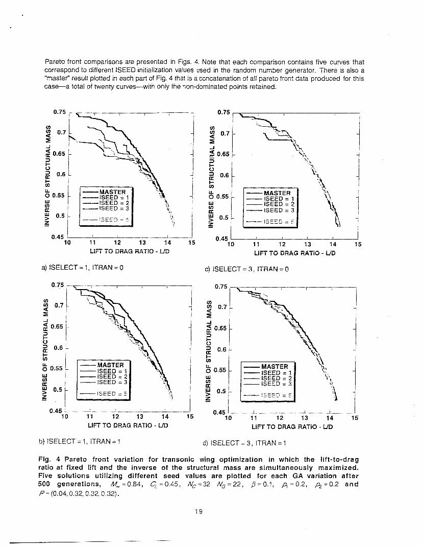
Pareto front comparisons are presented in Figs. 4. Note that each comparison contains five curves that correspond to different ISEED initialization values used in the random number generator. There is also a

case-a total of twenty curves-with only the non-dominated points retained. '(- , , I a s ~ e ~ .. - - - - . I + lci3ult plutt.=u -++-A I I ;- I caw --Ah I part of Fig. 4 that is a concatsnation of ail pareto frmt data produced !cr this

0.75

cn 8 0.7 E A - 0.65 3 I-

I 1 I 0.75

I

MASTER ISEED = 1 ISEED = 2

-1SEED = 3

0.45 5 1 11 12 13 14 15 10 0.45 1 I I I

11 12 13 14 15 10 L iF i TO DRAG FiAiiO - iiE

a) SELECT = 1, ITRAN = 0

I I

I 1 I

1 I

v) 0.7 1 I a

& 0.55 UJ a >" 0.5

F I i, I

0.6 1 -

i I- cn LL 0 0.55 ,- w cn II: >" 0.5 I

MASTER ISEED = 1 ISEED = 2 ISEED = 3

-[SEED = 5

- MASTER ISEED = 1 ISEED = 2 - S E E D = 3

,>=E:: = :

- - __ I - -

I I I 0.45 I I 10 11 12 13 14 15

0.45 1 I I I I 11 12 13 14 15 10 U t 7 TO DRAG RATiO - UD LIFF TO DRAG RATIO - U D

b) !SELECT = I , iT3A.N = 1 u") ISELECT = 3 , fTRAN = I

Fig. 4 Pareto front variation for transonic wing optimization in which the lift-to-drag ratio at fixed IEt and the inverse of the structural m a s s are sirnultaneclusly maximized. Five solutions utilizing different s e e d values are plotted for each GA variation after 500 generations, @,=0.84, CL=0.45, Nc=32 NG=22, B=O.i , p,=0.2, f i=O.2 a n d P= (C.C3,0.32,0.32,3.32).

19

There are several interesting features to note in this series of pareto front comparisons:

First of all, the vaiiation in level of ConveigeXe across the :a+x.s !SEED ~alues is quite striking, especii!!y for the cases invoiving greedy selection without gene space transiormation, iSEiECT = i, iiRAlzi = 0 (Fig. 4a). For these cases, the optimal lift-to-drag ratio point on the pareto front converges consistently in the number of generations allotted for this computation, regardless of the ISEED value, but the minimum structural mass point does not converge consistently.

This situation is improved, somewhat, for the ISELECT = 1, ITRAN = 1 case (Fig. 4b) where the best structural mass endpoint values are obtained. However, this latter set of curves suffers dramatically in the middle portion of the pareto front where the two objectives form trade-offs with each other.

The best results for this multi-discipline isolated-wing optimization are realized wnen bin seiecrion is utiiized, iSEiECT = 3 (Figs:4c ana 4aj. The pareto ironis for both sets of curves iiiat ijtiiize bin selectiofi more closely approximate the master curve than their counterparts using greedy selection. The set of curves in Fig. 4c-the ISELECT = 3, ITRAN = 0 case-are overall the best. Nevertheless, the minimum structural mass point for this set of computations still experiences inconsistency in convergence.

Convzigznze history comparisons for each of the pareto front curves presented in Figs. 4 are presented in Fig. 5. Computation of the pareto front error was achieved using the area error norm described above. The master pareto front displayed in Figs. 4 was used as an approximation to the “exact” solution. In addition, for each set of convergence history curves displayed in Figs. 5 there is an average convergence history curve plotted (the dashed curve), which is computed by arithmetically averaging each point in the conveigznce h ; s t q ! data file.

Note that occasionally the convergence histor\; ermr increases with gsneration. This usually occurs early in the convergence process when the pareto front is still crudely defined with a small number of discrete points and is explained in the series of sketches shown in Figs. 6. Figure 6a shows a hypothetical two- objective pareto front, both the exact curve and a crude approximation to it that might exist after the search has proceeded for n generations. Figures 6b and 6c show two different scenarios for what the pareto front might look like after n+ 1 generations.

in both scenarios a single new point has been added which neither dominates nor is dominated by any of the previously existing points on the pareto front. In scenario 1 the new point’s placement is less advantageous than that of scenario 2. Nevertheless, both new points are possible outcomes of the genetic algorithm search process. Despite the fact that scenario 1 represents an “enrichment” of the pareto front, the area error norm actually increases in going from the nfh generation to the n+lSt generation. This is why the area error norm occasionally jumps-either up or down-during solution evolution.

i

i

There is a moderately large amount of variance in each of the convergence history curves displayed in Fig. 5. This emphasizes the point that genetic algorithms are stochastically based. Comparison of results, especially convergence efficiency results, must be made with the proper amount of siatisticai averaging in place. Results from each MOGA variation demonstrate this conclusion.

I I 1

j I

1 i 1 I ,

l

a

a

0 0.1

0 K w I- Z

a L

---_ I

0 '

a I-

I- I I / i ( - - -AVERAGE

' - I D C C D = 5-

I I 0.01 I I I

0 100 200 300 400 500 GENERATION NUMBER

a) ISELECT = 1, ITRAN = 0

I I I

l I I

E 0 K ILI i 2

a

0.1 L 0 I- w a a n

- - -AVERAGE

0.01 I- 1 I I

0 100 200 300 400 500 GENERATION NUMBER

b) ISELECT = 1, ITRAN = 1

0.01 1 t I

0 100 200 300 400 500 GENERATION NUMBER

C) ISELECT = 3 , ITRAN = 0

Fig. 5 Convergence efficiency comparisons for transonic wing optimization in which the lift-to-drag ratio at fixed lift and the inverse of the structural mass a r e ~ i m ~ l k i f i ~ s i i s l y mz;~imizzb. Five sofotions uti!izing different seed va!ues sre p!otted f e r each GA variation, I!!- =0.84, C, =0.45, Nc=32 NG=22, p=O.l, p, =0.2, &=0.2 a n d P= (0.04,0.32,0.32,0.32).

The averaged convergence history efficiencies for each of the four MOGA variations studied herein are presented on the same set of axes in Fig. 7. Note that the two variations that utilize bin sele, ction are both faster than their greedy selection counterparts, achieving more than an order of nagnitude reduction in the area error norm after 500 generations. The gene-space transformation variation produced mixed results, being slightly faster wheri used with greedy selection and slightly slower when used with bin selecticn.

2 ;

0.2 .

0 0.2 0.4 0.6 0.8 1 7

OBJECTIVE 1

-TRANS + BINNING

1.2

1

0.8 n Y 2 E 0.6 w _I

0.4 :

0.2

0

NEW POINT

0 0 2 0 4 0.6 0 8 1 1.2

OBJECTIVE 7

a) Baseline, pareto front b) Pareto front after n + l after n generations. generations (scenario i j.

0.4

0 u 0.2 0.4 0.6 0.8 1 1.2

OBJECTIVE 1

cj Pareio ironi aiier n + i geiieiatioiis jsceiiaiie 2).

Fig. 6 Sketch of pareto front convergence history process showing two different advancement scenarios.

I

Computed results for the two-objective isoiated-wing optimization problem taken from the endpoints of a suitable SELECT = 3, ITRAN = 0 pareto front are displayed in Figs. 8-10. Figure 8a shows the upper surface Mach number contours for the minimum drag point (at fixed lift), and Fig. 8b shows the same view for the minimum structural mass point. Note the extreme suction pressure (high Mach number) upstream of the shock wave in Fig. 8b. This is caused by a large amount of flow expansion on the forward part of the wing and results in a much stronger shock wave than the solution depicted in Fig. 8a.

This situation can be viewed in a more quantitative way Dy looking at cross-sectional plots of the pressure coefficient, which are displayed in Figs. 9 for three spanwise stations-y/b= 0.21,0.51,0.78. In each plot the pressure Coefficient for the two pareto front endpoints-minimum drag and minimum structural mass-are displayed. From this series of figures it can be Seen that the minimum drag case (solid curves) has a greatly reduced shock strength relative to the minimum structural mass case (dashed curves).

!

I : I

22

Both soiu:iol;s have the same to:ai iift. Despira this, the spanwise disiribution of li% is diiierent between tne two cases. This can be seen from Figs. 9 by carefglly examining the arws circumscribed by each

more area inboard ana iess outboard reiaiive io the minimum drag point. This tends to move the center of pressure inboard for the rninirnurn struckml T;IZSS solution and t h u s , reduces the moment m through which t h e wing lift acts. This, in turn, reduces the wing root bending moment and ~ I I G W S for a lighter

c:~ss-secti=nal pressure c~eir ' ic ie~t pi&. The mizimni? cti~ctt lrs! mass co!utinn (~_~zshpd c~n/psI rnntzins I --..--...-

- A - ~1

Min drag 1 bj ?Gin s t ruc tura i mass

Fig. 8 Upper s u r f a c e Mach number contours for a t r anson ic wing optimization in w h i c h t h e d rag a t fixed l i f t a n d the s t ructural mass a re s imul t aneous ly minimized, lSELECT=3. I T ~ A N = c , = G.G, c, = 0.45. mfi = 32 lv, = 22 , R = O . l . p=02, & = 0 2 a n d P= (0.04.0.32.0.32,O 32).

1 -

I j

- u 5 L 0 0 2 0 6 0 6 0 8 1

NORMALIZED AXIAL DISTANCE - xic NORMALIZED AX:AL D S T A N C E - d: ..IORMAL!ZEC AXIAL DISTASCE - xjc

0 (1.2 0.4 0.6 6.8 T

Fig. 9 P r e s s u r e coeff ic ient bistribztions at sefecte.f spaa;wiss s i a i i ~ n s for t h e wirr g optimization problem presented in Fig. 8 showing d i f f e rences be tween the two p a r e l o front endpoints, CL = 8.45, ,*.& = 32 F V , = 22. ,2 = 0.7. q = 0.2

iSELECT=3, iTRAN = 0, Idx = 8.64, ,r2 = 13.2 and 3 = (3.04, '3.32, 9.32, tZ.32).

I 9 7

Another important attribute in this multi-discipline optimization problem is wing thickness-especially at the wing root. Selected airfoil cross-sectional profiles are presented in Fig. 10 at y lb = 0.0, 0.48,0.98 (wing root, mid-span, wing tipj. Profiies for both pareto front endpoints-minimum drag jsoiid curvesj and minimum structural mass (dashed curves)-are presented. Note that the vertical axis had been greatly expanded to facilitate viewing of the results, and that each profile is displayed in rigged position with wing twist included. For this set of computations the minimum-drag root-airfoil thickness is the minimum allowed by the geometric constraints and the minimum-structural-mass root-airfoil thickness is the maximum allowed. This is as expected. A reduced wing-root thickness helps reduce drag by reducing shock strength and thus reduces wave drag. An increased wing-root thickness helps to reduce structural mass by more efficiently supporting the wing root bending moment with a box beam that has increased depth.

Fig. 10 Selected airfoil profiles in rigged positions-at y/b=O.O, 0.48 and 0.98-for t h e transonic wing optimization problem of Fig. 8 showing differences between the two pareto front endpoints, (note the expanded z/c scale), ISELECT = 3, ITRAN = 0, M-zO.84, C,=O.45, N,=32 N,=22, p=O.l, p,=0.2, f i = @ . 2 and P=(O.O4,0.32,0.32,0.32).

The next set of computed results involves a two-objective optimization for a wing-fuselage configuration flying in the transonic flow regime--- = 0.84. The two objectives-lift-to-drag ratio at fixed lift and the ccnfiguration's volume-are simultaneously maximized by the previmsly presented MOGA optimizaticn procedure. As before, the aerodynamic lift-to-drag ratio is evaluated for each candidate design, that is, for each chromosome, using the TOPS full potential solvef" by iterating on angle of attack to obtain the lift-to- drag ratio ai the specified value of lift- C, = 0.45.

!

The wing-fuselage volume computation utilizes a straightforward algorithm that divides the fuselage into a series of cross-sections, computes the area of each cross-section using a simple triangularization and then computes the volume by integrating along the fuselage using trapezoid integration. The wing volume is computed using a similar algorithm that is deactivated for those wing cross-sections that lie inside the fuselage.

There are several reasons lift-to-drag ratio (at fixed lift) and wing-fuselage volume have been chosen as the twc) ohjecti\ve functiclns fer the present optimization problem. First of a!! there is a c!ear-cut cclnflict between these two objectives. When the volume is maximized the lift-to-drag ratio suffers and vice versa.

24

Thus, we have a classical engineering trade-off problem. How the MOGA performs on such a problem with real-world objectives is the key aspect of this study, not the development of new aeronautical engineering cmcepts.

In addition, the vehicie volume was chosen as an objective because it is an easy quantity to understand, The direct computation of maximum volume is easy to perform, thus providing a simple check for the results obtained by the GA-at least for one endpoint on the pareto front. This problem is interesting in that it is complicated by iransonic-flow shock-wave-indticsd non!ineaii:ies and by a farge number zf decision variables that have large sensitivity variations.

The present wing-fuselage parameterization with two wing defining stations, N, = 2, as described above, consists of 66 parameters. Airfoil defining station one is at the wing root and station two is at the wing tip. There are 24 A f values used to define the fuselage-six equally-spaced axial stations, each with four equally-spaced meridinal locations. The axial positions are located at x ic= O . i i , i .43,2.i 4,2.86,3.57,4.29 where the fuselage length is fixed at x,=5.0. The meridinal positions are located at v, = -go", - 30", 30", 90" where q~ = -90" corresponds to the fuselage keel line and p = 90" corresponds to the crown line.

Maximum and minimum constraint values for each of the geometric parameters, as well as masking amy values, are given in Table. 4. As can be seen, 43 of the 66 genes that make up each chromosome have masking array values of one, and 23 have values of zero, that is, only 43 genes are actually modified during the optimization process-& = 43. Note also that the max-min values associated with each of the A r values are not symmetric about zero. Along the keel and crown lines, for example, any A f value averaged between the max and min constraints, will be positive, and along the other meridinal stations (along the fuselage side), the same averaging will produce negative values. The inax and min A f CGnS:iZiRiS V<CiS chssen in iiiis way io keep rne vertical extent of the fuselage from becoming too small. A difficulty arises in the wing-fuselage line of intersection computation if the intersection line contacts the symmetry plane. This results in fuselage designs that bave depth-to-width ratios that generally exceed unity-sometimes by a substantial amount.

The first wing-fuselage optimization results are presented in Figs. 11 -14. For these results the freestream Mach number is 0.84 and the lift coefficient is held fixed at 0.45. The tolerance on the lift iteration is &1%, but in most cases the error is much less. The second binning selection algorithm with endpoint retention is used, lSELECT=4, and the gene-space transformation procedure is turned off, lTRAN=O. Both of the mutation probabiiities are iixed at 0.2 and P= (0.04,0.32,0.32,0.32).

This optimization uses 34 chromosomes for each generation. The first element of the P vector is set such that two passthrough chromosomes are chosen during each generation-always the pareto front endpoints-the current minimum drag and the maximum volume chromosomes. Thus, 32 modified chromosomes require new function evaluations during each generation. These function evaluation computations are efficiently performed simultaneously on 32 processors of a parallel computer. The other three elements of the P vector are set to evenly divide the remaining ChiGr?iGSGi.iieS between the :h:se remaining modification operators-random average crossover, perturbation mutation and mutation (at least as close to even as possible).

Development of the pareto front as a function of generation number is displayed in Fig. 11. Note that the mwimum volume point on the pareto front, which occurs at a value of 1.42, converges quickly, achieving 96% of the theoretical maximum in as few z 50 generations, while the minimum drag point is slower in convergence. This characteristic, displayed in Fig. 11 for one ISEED value, occurred for every ISEED value utilized and is due to severai factors.

25

Table 4. Maximum and minimum gene constraints along with masking array values for the wina-funnlaae notimizatian arablem.

First of all, the volume objective depends on most of the genes in a simple way. For example, if one of the 4r genes is increased, while all other genes are held fixed, the volume increases in a proportionate amount throughout the range of that gene’s variation. This behavior exists no matter what value the other genes possess. In addition, the maximum volume values of many genes in the present wing-fuselage parameterization-certainly all of the fuselage 4r values-are at their upper constraint values. Finding an optimum on the design space boundary seems to be easier than finding an optimum within the design space interier.

The drag objective depends on the various genes in a more complex manner than that of vehicle volume -especially for this wing-fuselage problem. Interrelated and simultaneous changes in several genes are typically required in certain regions of the design space to achieve improvement in the drag objective. For example, when z, is changed the position of the wing-fuseiage juncture changes. To achieve optimai drag performance the wing-fuselage area ruling needs to be simultaneously adjusted, and this requires coordinated changes in various elements of the array. Which elements have to be changed and by how much depends on the value of 2,.

26

j

The slow convergence of the drag pareto fror,t endpoint for the present wing-fuselage problem, relative to the second objective, was not observed in the previous problem. In fact, the second objective for the previn~~s isolated-wing optimlzatinn prob!em-minimization nf the structura.1 mass-was slower than that of the drag. There are hvo reasons tor this appaiGfit inconsistency. Firs: of all, the complex interdependence of the drag objective on wing placement and the ensuing fuselage area ruling issues do not arise in the isolated-wing problem. Secondly, the dependence of the structural mass -on the gene value distribution for the isolated-wing problem is every bit as complicated as for the drag objective-perhaps more so. That’s because the stiudural mass depends on both the wing thickness distribution, especially near the wing root, as well as the wing pressure distribution-the latter quantity setting the wing’s center of pressure and thus the moment arm for the wing root bending moment.

1.4

W 1.3 I 3 -i

p 1.2 a LU N 2 1.1 q I K 0 1 z

0.9

I / , K”

0.8 ! I I I I I I 5 E i e 12 14 16

LIFT/D R A G

1 7 . - t i ‘ rmi . .

b7 1 -1

w y.* - c.5

i

0 0.2 0.4 0.6 0.8 1 AXIAL DISTANCE - x/c

Fig. 11 Pareto front convergence and solution structure for a wing-body two-point optimization involving drag minimization and volume maximization both at constant l ift ,

3, = 0.2 m d P= (0.@4,0.32,0.32,0.32). Wing sectional pressure distributions are presented at three positions along the pareto front, A) maximum volume, B) intermediate, C) minimum drag.

GzO.45, M- =0.84, lSELECT=4, ITRAN=O, N0=2, Nc=34, 4 = 4 3 . BzO.1, pI =0.2,

Also displayed in Fig. 11 are several airfoil pressure distributions for three different solutions corresponding to three different locations along the pareto front, A) maximum volume, B) intermediate and C) minimum drag. For each solution two airfoil pressure distributions are presented-the first inboard near the wing-fuselage juncture ( y / b = 0.2) and the second near mid-semi-span (y/b = 0.6). The most obvious feature from these results is the change in shock strength as the pareto front is traversed. The maximum volume solution (A) contains strong shocks, both on the upper and lower surfaces of the wing, while the minimum drag solution (C) contains mild shocks on only the wing’s upper surface.

Upper surface Mach number contours for each of the three soluiions presented in Fig. 11 are dispiayed in Figs. 12. This series of figures shows the shock wave pattern variation on the upper surface of the wing- fuselage configuration as the solution transitions from the maximum volume pareto fcont endpoint to the minimum drag endpoint. For the maximum volume endpoint there are strong shock waves, not only on the wing, as seen in Fig. 11, but also on the fuselage near the nose and tail. The fuselage shock waves are caused by the GAS selection of minimum values ior ihe x, ana x, genes. These values maximize the

27

vehicie volume. but cause shock waves to form ai Sot? the fuseiage nose and tail due to excessive over- expansior!

--= 1

A) Max volume solution B) Intemediate soIution C) Min drag solution

Fig. 12 Surface Mach number contours for the winglbody oi;tirnizaiior: pob lem presented in Fig. 11 at three positions along the pareto front.

As the soiution propaga?es along the i;Zi&o :ion;. tiading iiO!urne to obtain a redticbZ in drag, EZS:

noticeabie initial change is associated with the fuselage nose and tail fairings. By choosing larger values for x, and xT, the drag is decreased without sacrificing a iarge amount of volume. This can be seen by examifiirig the internediate ~~liri ion in Fig. 12 aiid noting-its position on the pareto h r ; t in Fig. 17. Fiiithei reductions in drag are achieved Va the complex task of fuselage area ruling in the vicini9j of the wing- fuselage juncture. Such a result is observed by looking at the minimum drag solution in Fig. i2. More on this, including a comparison of selected fuselage cross-sections will be presented subsequently.

Pressure distributions along the fuselage for the three solutions described in Fig. 11 are presented in Figs. 13. Results are plotted along three fuselage meridinal stations-the keel line (9 = -goc), the side, { q = Os) ax! the crcwn fine ( q = W). Each cf these sslutions invclves 2 high rctlntnd ?.ring. t h i l is, the MOGA optimizer has chosen a high mounted wing, regardless of the solution’s position along the pareto front. More will be presented on this aspect subsequently. Because of this the side fuselage pressure distribution (0 = O“) is plotted a!ong a continnous meridinal ! i x the! !ies k ! o w the wing for each of these three sciuticns. In addition. hlach nunSer ccntours BS viewed from the fussiage‘s side are also dispiaysr! in Figs. 13.

- ! I I.

2 3

1.5

-KEEL LINE - S I D E v= 1 ; CROWN L I N E 1

I

0.2 0.4 0.6 0.8 1 0

AXIAL DISTANCE ALONG FUSELAGE - WL

3; %i3Xii'ilLjm VoiUfiE SOiUfiGjj .

1.5

- Vu 1 - - - - - - C R O W N LINE

+ w

i

= ! 0.5 -

0.2 0.4 0.6 0.8 1 0

AXiAL DISTANCE ALONG FUSELAGE -- x/L b) !-s=--=-&:-*= -.-!::A!-=

: i i L c & iiicuiatc ~ U I U L ~ U I I .

Fig. 13 Fuselage pressure distributions for t h e wing!l;cdy =p+;-;--+' ~ ~ c ~ i ~ L a L ~ ~ ~

presented in Fig. 11 et three positions ainng t h e pareto front. problem

By compaiing each pa': of Figs. 7 3 with the corresponding part in FIGS. 12, it c m be SGSR that tcis de;lth <zf the fuselags! a measured from keel to ciawn is much large: than mice t h e half-width for any given iongitudinai siation. This is a direct result of the choices mads in settinG I+ the constraints for the 1; a:iaj..

h a t l i e eiongated in the z-drection. This situztie:: is pesenterl in a mere quantitativs way in Fig. 74, k., 3c \ f l r 2 Q .._I -., ~ l r a a ~ } ~ _-_ diSCYSSec! in t h s filselage parameterization section, 2nd produces fuselage cross-sec:i3ps

A series of fuselage cross-sections are presented in Fig. 14 for the two-objective optimization problem displayed in Fig. 11. For each cross-section there are two curves plotted. The solid curve corresponds to the solution sbtained zt the minirur-drag pareto frent endpoint, 2nd t he dashed curve corresponds to the solution obtained at the maximum-voiume pareto front endpoint. Foi this sdiition the wing root leading edge is placed at (x,, yR, z,) = (1 .5,0.0,0.15). Note that x, = 1.5 and yR = 0.0 are values set at the beginning of the computation and are held fixed, and that z, = 0.1 5 is a value selected by the MOGA optimization for this particular chromosome from the range, -0.1 5 I z, 50.1 5 (see Table 4). The only fuselage cross-section in Fig. 14 that actually intersects with the wing is the one at xIc= 1 5 4 . As seen from Fig. 14, the fuselage cross-section is drawn before the wing intersection is included.

-

From this set of plots it is easy to see how the fuselage was area ruled in the vicinity of the wing-fuselage ,-. ii inrti .---.- irn ?c nhtain .. tho ...- final nmni int cf drzs rerf-icti~n; Vnli-Jrne is subtracted alona the upper portion of the fuselage near where the wing intersects, creating “pear-shaped” cross-sections in this fuselage location. Every cross-section from the maximum volume solution contains more area than the corresponding minimum drag cross-section. Each of the A f values for the maximum volume solution is individually maximized.

-0.6 0 0.1 0.2 0.3 0.4 0 0.1 0.2 0.3 0.4 0 0.1 0.2 0.3 0.4

YJC Y/C Y l C

0 0.1 0.2 0.3 0.4 0 0.1 0.2 0.3 0.4

Y l C Y l C

Fig. 14 Selected fuselage cross-sections for the wing/fuselage Optimization problem sf Fig. 1 I showing diffe:ences between the t ~ n ;arete frorrt endpaints, Ci = 0.45 M,=O.84, lSELECT=4, lTRAN=O, N,=2, Nc=34, NG=43, p=O.l, p,=O.2, &=0.2 and P= (0.04,0.32,0.32,0.32).

Convergence efficiency !or the two-objective wing-fuselage optimization problem just discussed-drag minimization and volume maximization (both at fixed lift)-is presented in Figs. 15 and 16. Figure 15 shows the previously discussed area error norm plotted versus the number of function evaluations for three different convergence histories involving three different population sizes-34, 66 and 1 30 chromosomes, respectively. Each curve is averaged over two ISEED values in an attempt to eliminate some of the statistical variation. As can be seen each cofiveigence history is nearly ?he same, indicating that convergence is not afunciion of population size. This is compatible with the results presented in

30

Ho!st and Pulliami5 where a number of model problems were used to evaluate GA convergence for two- objective optimization.

For this set of computations the number of processors used io perform the function evsftiations is equal to the number of chromosomes requiring function evaluations. There are always two passthrough chromosomes. The remaining chromosomes-those needing modification-are arbitrarily divided into three groups of equal size-or as close to equal as possible. One group is modified using crossover, the second tising perturbation mutatior; and the thiid using global mutation. Since, twc passthrcugh chromosomes are utilized for each population, the number of processors required to perform function evaluations is 32, 64 and 128, respectively. Using an increased number of chromosomes to define a given population allows an increased number of processors to be used for the optimization problem and thus, improves turn-around efficiency.

Figure i 6 presents a comparison of ihe six pareto ironis computed fioiTi the coiiveigsiiee efficiency stucly presented in Fig. 15. These results are statistically similar to previous results presented in this section and suggest that there is no significant effect of population size on the final solution. Care should be taken in evaluating this conclusion, as the number of solutions needed to construct a proper statistical average has not been uiiiized in this case due to computer time limitations.

100

U B I!? a 1 1 1 I

t- 2 0 K U

0 t- w l CK 4 P

0.1

I I f

Y-.

I I

0 5000 10000 15000 20000

NUMBER OF FUNCTION EVALUATIONS

Fig. 15 Pareto front convergence history comparisons for three population sizes, each averaged over two ISEED values, wing/fuselage optimization problem. C, = 0.45, M- = 0.84, ISELECT = 4, iTRAN=O, N0=2, N ~ = 4 3 , B=O. I , P,=O.2 , fi = 0.2.

1-5 I

I I

1 0.7 '

5 10 15 LIFT TO DRAG RATIO

Fig. 16 Pareto front comparisons for three population sizes, each with two different SEED values, wing/fuselage optimization problem, C, = 0.45, hL =G.64, lSELECT=4, lTRAN=O, N0=2, NG=43, pzo.1, /q =0.2, =0.2.

It is of interest to study how the individual genes vary along the pareto front. Selected genss from the wing-fuselage optimization problem described in Fig. 11 are plotted along the pareto front in Figs. 17 and 18. In particular, they are plotted as a function of the pareto front's first objective, lift-to-diag ratio. Each gene is normalized and then plotted so that it varies from 0 to 1, For many of the curves the discrete points are plotted along with a smoothed result. in some cases, where the number of curves on a single set of axes is large, only ihe smoothed curie is plotted.

31

1.2

1

W 2 < 0.8 > W 5 0.6 d 0 t 0.4 - J a 2 0.2 - z

0

-0.2

MAX VOLUME MIN DRAG

4 6 8 10 12 14 16

LIFT TO DRAG RATIO

MAX VOLUME MIN DRAG

a) x-ltrcatioii e: sirfoil maximum thickness on the lower surface at t h e wing tip, GENE,, = xlo,.

1.2 I

GENE 1 4 SMOOTHED 1

< 0.8 >

b) Airfoil trailing edge angle at wing r o o t and tip, GENE, = ate, and GENE,, = ate,.

1.2

1

W 3 < 0.8 > w

d 0 2 0.4

5 0.6

- -I a = 0.2 p

0

-0.2

I o GENE 15 I 1 ci GENE 16

MAX 1~~~~~~ MIN DRAG I I I

8 10 12 14 16 4 6

LIFT TO DRAG RATIO

c) Airfoil twist at ..,ng :=et and GENE,, = 8, and GENE,, = 8,.

1.2 o GENE 17 o r>

I GENE 18 -SMOOTHEDJ

1

W 5 0.6 i3 0

0.4

0

0 G O 00 O Q

ma

d) Vertical wing posit ion ( GENE,, = zR), fuselage nose length (GENE18 = xN) and fuselage boattail length (GENE,, = xT).

Fig. 17 Normalized gene distributions along the pareto front from selected posit ions within each chromosome, wing/fuselage optimization problem, C, = 0.45, Mm = 0.84, ISELECT = 4, ITRAN = 0, No = 2, N, = 34, N~ = 43, p = o.i, ,q = 0.2, & = 0.2, P = (0.02,0.33,0.33,0.32).

The first general observation is that a significant amount of statistical variation exists in many of the genes 2s they vary across the pareto front. Some genes wi!dly Csci!!ate withoit any discernible pattern. The x- location of the wing-tip lower-surface maximum thickness-xlo,, gene number 11-is such an example. Of the 43 av.i!able genes, xlo, contains the most variation. This gene is plctted in Fig. 17a and is Seen i0

3 2

favor the maximum value in its allowable range. Nevertheless, it takes on many other values in a seemingly haphazard fashion.

TL- I I it= re..- 1ea3on for this bShZi6oi is stiaighffoxard. This gene has fittie ingact =:: either cbjective being

optimized and thus has iirtle impact on the pareto front. Any value is generally acceptable at any location along the pareto front. To test this observation several chromosomes were selected from the pareto front for which xlo, was against one of its constraints. The value of xlo, within that chromosome was then moved to the opposite ccnstraint without changing any other gene value, and 2 new solution was computed. The resulting design-space point moved little and was still a member of the pareto front. Ideally, such a parameter shouldn't be utilized as a gene in the optimization process. In reality it is difficult to know a priori which genes will behave in this way and which will not.

Oiner parameters pioiiea in Fig. i i inciude ihe iraiiing esiga iiiiyie si ii-ie wiiig icct sfid tip {Fig. t h ~ a ih i i PtiSt a: the Wig i& 2nd tip (Fig. 1 7 ~ j , and the :.e,?Ical W~XJ mo~::ting positbn, the length 2nd the boattail length (Fig. 17d). All of these gene parameters have reasonably controlled variations across the pareto front.

Figure 18 presents the variation of each of the Ar parameters for the wing-fuselage optimization problem--all 24 of them-across the pareto front. As already discussed, the A r parameters are organized into four meridinal stations, each with six longitudinally distributed values. Each meridinal station is plotted on a separate set of axes in Fig. 18. Figures 18a, 18b, 18c and 18d show the 4 f longitudinal variation along Q, = -goo, - 30", 30" and 90°, respectively.

1,s expect&, &I A;r v&ups g ?he .~zyi,m.um yolgme endpoint o.r! thg par&c front lip at their mzyimy.m. constraint limits. Moving away from this endpoint, many of the A f values decrease from their maximum ccnstrain! va!ues 2nd zttain intermedia@ values. This is especia!!y true tor the 4r values along the IJ = 30" and p = 90" meridinal stations, where reductions in the various 4r values have been determined by the MOGA optimizer to achieve optimal fuselage area ruling in the vicinity of the wing-fuselage juncture.

It is of interest to study the effect of wing placement on the overall wing-fuselage optimization problem. In the cases presented above, the vertical wing position, zR, is constrained to lie between -0.1 5 and 0.15, while x, and yR are fixed at 1.5 and 0.0, respectively. As a result of the optimization, the value of z, is chosen to lie at or near its upper constraint value, z, = 0.1 5, over the entire pareto front (see the variation of gene i 7 plotted along the pareto front in Fig. 17d). In other words, a high wing intersection is favored by the optimization regaraiess oi position on the pareto iront-at ieast in the context of the present design space construction.

Figures 19 and 20 present results for a wing-fuselage optimization in which the wing intersection is constrained to be low mounted, that is, the value of z, is constrained io be -0.1 5. All other design space attributes and constraints are the same as in the previous wing-fuselage computations. This is implemented by setting the maximum constraint for z, equal to the minimum constraint, z, = -0.1 5, and by setting the corresponding z, masking array value to zero. Tnus, for this probiem, NG = 42, instead oi the previous value of 43. Note also that IC = 66 for this series of computations, tnat is, 64 processors were used in the optimization.

Figiire 1 S displajis ~o coiiipiited pai&o fr~r i ts fo i :he oiigind wing-fuselage ~ptimizatisn problem and ~ W G pareto fronts for the optimization that constrains the wing to be low-mounted. The two curves plotted for each case correspond to two different SEED values. As can be seen, the low mounted wing results are less efficient in the vicinity of the minimumdrag paretG front endpoint. The IGw-mounted case achieves essentially the same level of drag, but only when vehicle volume is reduced. Note also that this effect is large in comparison to the statistical vai'iation that exists between the two ISEEL7 computations from each solution citegory. The effec? of + on the maximum vn!ume pareto front endpoir,t is negligible.

33

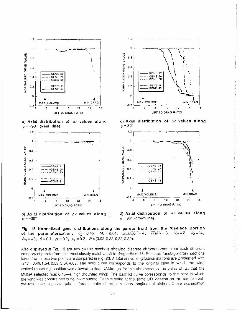
MAX VOLUME MIN, DRAG

i I

I

! U 0.8 1 >

4 MIN DRAG

-GENE 22 - -- -GENE 26 . . - - . G E N E 30

GENE .>e ------- GENE 42

-GENE 23 - - - - - G E N E 28

--- GENE dn - GENE 35

4 MAX VOLUME

- 1 4 4 .n 7 I I I I I I

4 6 8 10 12 14 16

LIFT TO DRAG RATIO

c> .Axial d i s t r i b ~ f i ~ n of br values along V, = 30"

1.2

1

W 3 J 0.8 > W 5 0.6 a n w 0.4 N

a

J U

0 2

$ 0.2

0

-0.2

! '

-GEFiE 23 - - -GENE 27 -. - - - GENE 31

I

MINI DRAG 4

MAX ,VOLUME I I

4 6 8 10 12 14 16

LIFT TO DRAG RATIO 4 6 8 10 12 14 16

LIFT TO DRAG 'RATIO

d) Axial distribution of Ar values along cp = 90" (crown line).

b) Axial distribution of A r values along = -30"

Fig. 18 Normalized gene distributions along the pareto front from the fuselage portion of the parameterization, C, =0.45, /isF, = 0.84, SELECT = 4 , I I n n l \ = o , ' T n A h ' & = 2 , qc=34, NG=43, p=O.l, ~ 0 . 2 , h z 0 . 2 , P=(0.02,0.33,0.33,0.32).

Also displayed in Fig. 19 are two circular symbols showing discrete chromosomes from each different categery c f p a r e; , tn f, rnn+ i L ++at mcst clcseiy match a Lift-to-drag ratio ~f 13. Se!ected f.se!=lge cress sections taken from these two points are compared in Fig. 20. A total of five longitudinal stations are presented with x I c = 0.49,1.54,2.59,3.64,4.69. The solid curve corresponds to the original case in which the wing veflical mounting position was allowed to float. (Although for this chromosome thz value of zR that the MOGA selected was 0.15-a high mounted wing). The dashed curve corresponds to the case in which the wing was constrained to be low mounted. Despite being at the Same UD locaiion on the pareto front, the two area rulings are quite biffereiii-quiie different at each iongi:i;diml &:ion. C t ~ s e examinaticn

34

shows how the MOGA modified the area ruling to account for the shifted wing mounting position, taking volume from the upper fuselage for the high-mounted case and from the lower fuselage for the low mounted case. R is also obvious that the fuselage associated with the low-mounted wing contains a smaller StTGUGt Of Volume as is C G R S i S h t With Fig. 13.

1.5 I 1

LIFT TO DRAG RATIO

Fig. 19 P a r e t o f ron t c o m p a r i s o n s for twa different wing-fuse lage opt imiza t ion cases: a ) base l ine in which wing position is al lowed to float ( - 0 . 1 5 S ~ ~ 5 0 . 1 5 ) and b) wing fixed in t h e low-wing pos i t ion ( zR = -0.15). Each computa t ion pe r fo rmed with two ISEED v a l u e s , C, = 0.45, M- = 0.84, ISELECT = 4, ITRAN = 0 , No = 2, Nc = 66, NG = 43/42, /3 = 0.1, p, = 0.2,

=0.2, p= (U.UZ, '- - - 0.33,0.33,0.32).

I 1

I I 1 i

1 I

i I I 1

I -0.6 L A

0 0.1 0.2 0.3 0.4

Y i S

Fig. 20 S e l e c t e d

0 0.1 0.2 0.3 0.4 y i c

l l i , ,

0 0.1 0 2 0.3 0.4 y i c

fuselage c r o s s - s e c t i o n s for t h e

r - ' ' ' I

, ' - L I

0 0.1 0.2 0.3 0.4 y i c

0 0.1 '0.2 0.3 0.4 y l c

two wing/f use la ge o p t i m iza t io n p r o b l e m s of Fig. 19 s h o w i n g d i f f e r e n c e s b e t w e e n t h e two s o l u t i o n s a t L i D = 1 3 : a ) baseline ir; wh ich wing pos i t ion is al lowed t o float ( - 0 . 1 5 5 ~ ~ S O . 1 5 ) a n d b) wing fixed i n t h e low-wing pos i t ion ( zE = -0.15)? C, =0.45! M, = 0.84, ISELECT = 4, ITRAN = 0 , ID = 2 , Nc=66, NG=43/42, Bz0.1, ~ ~ 0 . 2 , ~ ~ 0 . 2 , P=(0.02,0.33,0.33,0.32).

3 5

Conclusions

A multi-objective genetic algxithm (MOGA) optimization prccedure, with severa! se!ection a!gorithm options ana a new gene-space transiormation procedure, has been presented. ii uses ieal-fii-imber encoding to represent all design space decision variables as genes and populations of fixed size to go from generation to generation. Four modification operators are utilized to advance from one generation to the next. They include passthrough, random average crossover, perturbation mutation and mutation. The standard output for this approach is a pareto front, which includes the best solutions from each objective, as well as a range of optimal “tradeoff” solutions in between.

The MOGA optimization procedure was utilized to determine a number of multi-objective optimal solutions for two problems. The first involved a transonic wing lift-to-drag maximization (drag minimization) coupled with the simultaneous minimization of structural mass (ali at fixed iiitj. Tile second invoived a transonic wing-iuseiage iiii-io-drag maximization (drag minimization) coiipied with the simiilianeoiis iiiaxiiiiizztion of vehicle volume (all at fixed lift). In every case the GA optimization process was convergent. However, some of the GA variations studied converged more rapidly than others.

Of the two selection algorithms compared-greedy selection and bin selection-the latter produced the most efficient ccnvergence acrcss all of t h e problems studied. The gene-space transformation procedure produced mixed results in the area of GA convergence efficiency. In some cases it was moderately faster, for other cases moderately slower.

A limited parallelization efficiency study was performed involving the use of 32 to 128 processors. Population sizes ranging from 34 to 130 chromosomes were used. The present MOGA is essentially embarrassingly parallel with regard to the number of chromosomes used for each generation, and the number of chromosomes did not affect convergence efficiency of the MOGA scheme. Thus, the turnaround time dramatically decreased with increasing number of processors.

1.

I

2.

3. I

4. I

5.

6 .

References

Goldberg, D. E., “Genetic Algorithms in Search, Optimization and Machine Learning,” Adaison- Wesley, Reading, MA, 59-88, 1989.

Davis, L., “Handbook of Genetic Algorithms,” Van Nostrand Reinhold, New York, 1991.

Beasley, D., Bull, D. R. and Martin, R. R., “An Overview of Genetic Algorithms: Part I , Fundamentals,” University Computing, Vol. 15, No. 2., 1993, pp. 58-69.

Beasley, D., Bull, D. R. and Martin, R. R., “An Overview of Genetic Algorithms: Part 2, Research Topics,” University Computing, Vol. 15, No. 4., 1993, pp. 170-181.

Deb, Kalyanmoy, “Multi-Objective Genetic Algorithms: Problem Difficulties and Construction of Test Problems,” Evolutionary Computation, Vol. 7 , No. 3, 1999, pp. 205-230.

Van Veldhuizen, David and Lamont, Gary, “Multiobjective Evolutionary Algorithms: Analyzing the State-of-the-Art,” Evolutionary Computation, Vol. 8, No. 2, 2000, pp. 125-1 47.

3s

7. Jimenez, Jose, Cuesta, Pedro and Abderraman, Jesk , “Mixed Strategy in Genetic Algorithms: Domain’s Reduction and Multirecombination,” European Congress on Computational Methods in Applied Sciences and Engineering, ECCOMAS 2000, Barcelona, Spain, Sept. 2000.

8. Obayashi, S. and Tsukahara, T., “Comparison of Optimization Algorithms for Aerodynamic Shape Design,” AlAA J., Vol. 35, 1997, pp. 1413-1415.

9. Bock, K.-W., ”Aerodynamic Eesign by Optimization,” Paper 20, AGARD CP-453, 7990.

10. Hoist, T. L. and Pulliam, T. H., Evaluation of Genetic Algorithm Concepts using Model Problems, Part I: Single-Objective Optimization, NASA TM in preparation, 2003.

- 2

I I. Ziizier, E., T‘nieie, i. iaumanns, ivi., Fonseca, e. ivi. arid & Foitseca, b‘. G., “F6Ti~i i i ia i iC~

Evolutionary Computation, Vol. 7, No. 2, April 2003, pp. 117-132. Assessment of h l n lv~ul.~~~,ective *Itinhi Optitimizers: A:: analysis and Revie:.:,” !EEE Trznsacf,&s cn

12. Deb, K., Pratap, A. and Meyarivan, T., “Constrained Test Problems for Multi-Objective Evolutionary Optimization,” Proceedings of the First International Conference on Evolutionary Multi-Criterion Optimization, March 7-9, 2001, Zurich, Switzerland, pp. 284-298.

13. Van Veldhuizen, D., “Multiobjective Evolutionary Algorithms: Classification, Analyses, and New Innovations,” AFIT/DS/ENG/99-01, June 1999.

14. Lohn, J. D., Kraus, W- F. and Haith, G. L.: “Comparing a Coevolutionary Genetic Algorithm for Multiobjective Optimization, Proceedings of the 2002 IEEE Congress on Evolutionary Computation, May 2002, pp. 1 157-1 162.

15. Hoist, T. L. and Pulliam, T. H., Evaluation of Genetic Algorithm Concepts using Model Problems, Part 11: Mufti-Objective Optimization, NASA TM 2003-21281 3, Dec. 2003.

16. Laumanns, M., Thiele, L., Deb, K. and Zitzler, E., “On the Convergence and Diversity-Preservation Properties of Multi-Objective Evolutionary Algorithms,” Swiss Federal Institute of Technology (ETH), Zijrich, Switzerland, TIK Report No. 108, June 2001.

17. Deb, K., Mohan, M. and Mishra, S., “A Fast Multi-Objective Evolutionary Algorithm for Finding Well- Spread Fareio-Opiimal Solutions,“ Kanpur Genetic Algorithms Laboratory (KANGAL), KanGAL Report No. 2003002, Feb. 2003.

18. Knowles, J. D. and Corne, D. W., “Approximating the Nondominated Front Using the Pareto Archived evolution Stategy,” Evolution Computation, Vol. 8, No. 2, 2000, pp. 149-172.

19. Knowles, J. and Corne, D., “Properties of an Adaptive Archiving Algorithm for Storing Piondominated l‘ec?o:s,” lEEE Transactims cn E?d~tjonary Co,7?,nutatim, Vc!. 7, ?!o. 2, April 2003, pp. 100-1 16.

20. Parmee, I. C., Cvetkovic, D., Gonharn, C. R. and Mitchell, D., ‘Towards Interactive Evolutionary Design Systems for the Satisfaction of Multiple and Changing Objectives, European Congress on Computational Methods in Applied Sciences and Engineering, ECCOMAS 2000, Barcelona, Spain, Sept. 2000.

21. Marco, N, Dssideri, J.-A. and Lanteri, S., “Multi-Objective Optimization in CFD by Genetic Algorithms,” lnstitut National de Recherche en lnformatique et en Automatique, Research Report No. 3686, April 1999.

37

22. Naujoks, B., Willmes, L., Haase, W., Back, T. and Schutz, M., “Multi-Point Airfoil Optimization Using Evolution Strategies,” European Congress on Compufational Mefhods in Applied Sciences and E~gineering, ECCOMAS 2000, Barcelona, Spain, Sept. 2000. I

23. Quagliarella, D. and Della Cioppa, A., “Genetic Algorithms Applied to the Aerodynamic Design of Transonic Airfoils,” AlAA Paper 94-1 896-CP, 1994.

24. Vicini, A. and @uagliarella, D., ‘‘Inverse and Direct Air!oil Desigr, Using a Multiobjective Genetic Algorithm,” AlAA J., Vol. 35, 1997, pp. 1499-1 505.

25. Hamalainen, J., Makinen, A., Tarvainen, P. and Toivanen, J., “Evolutionary Shape Optimization in CFD with Industrial Applications,” European Congress on Computational Methods in Applied Sciences and Engineering, EGGGivi A S ZSGG, Earceiona, Spain, Sept. X G G .

I

26. Epstein, B. and Peigin, S., “A Robust Hybrid GNROM Approach to multiogjective constrained Optimization in Aerodynamics,” 1 6th AlAA Computational Fluid Dynamics Conference, Orlando, Florida, AIAA Paper No. 2003-4092, June 2003.

I 27. Anderson, M., Burkhalter, J. and Jenkins, R., ‘‘Missile Aerodynamic Shape Optimization Using Genetic Algorithms,” J. of Spacecraft and Rockets, Vol. 37, No. 5, Sept.-Oct. 2000, pp. 663-669.

28. Anderson, M. and Gebert, G., “Using Pareto Genetic Algorithms for Preliminary Subsonic Wing Design,” AlAA Paper No. 96-4023-CP, 1996. I

29. Sasaki, D, Obayashi, S. and Nakahashi, K., “Navier-Stokes Optimization of Supersonic Wings with Four Design Objectives Using Evolutionary Algorithm,” AlAA Paper No. 2001 -2531, 2001.

30. Oyama, A., “Multidisciplinary Optimization of Transonic Wing Design Based on Evolutionary Algorithms Coupled with CFD Solver,“ European Congress on Computaiional A4eihods in Applied Sciences and Engineering, ECCOMAS 2000, Barcelona, Spain, Sept. 2000.

31. Ng, K. Y., Tan, C. M., ray, T. and Tsai, H. M., “Single and Multiobjective Wing Planform and Airfoil Shape Optimization using a Swarm Algorithm,” 41 st Aerospace Sciences meeting and Exhibit, Reno, Nevada, AlAA Paper No. 2003-45, Jan. 2003.

32. Obayashi, S., Yarnaguchi, Y. and Nakamura, T., “Multiobjective Genetic Aigoritnm for Multidisciplinary Design of Transonic Wing Planform,” J. of Aircraft, Vol. 34, 1997, pp. 690-693.

33. Oyama, A. and Liou, M.-S., “Multiobjective Optimization of Rocket Engine Pumps Using Evolutionary Algorithm,” AlAA Paper No. 2001 -2581, June 2001.

34. Benini, E., “Three-Dimensional Muiti-Objective Design Optimization of a Transonic Compressor ,-,I- uuiiipuiatiui tai Fluid Dinarnics Conference, Orland=, Flsrida, AlAA Paper Ne.

2003-4090, June 2003. Ro:or,” f

th A A A P ~ - ~ ~ ~ + - t ; n m - l 5

35. Oyama, A. and Liou, M., “Multiobjective Optimization of a Multi-Stage Compressor Using Evolutionary Algorithm,” AIAA Paper No. 2002-3535, 2002.

36. Rai, M. M., ‘Towards a Hybrid Aerodynamic Design Procedure Based on Neural Networks and Evolutionary Methods,” 20th AlAA Applied Aerodynamics Conference, St. Louis, MO, AlAA Paper No. 2002-31 43, June 2002.

37. Madavan, N. K., “Aerodynamic Shape Optimization Using Hybridized Differential Evolution,” 2 1 AiAA Appiied Aerodynamics Conference, Griando, Fi, AiAA Paper No. 2003-3792, june 2003.

38

38,

39.

40.

41.

42.

43

44.

45.

46.

47.

48.

49.

50.

Giotis, A. P., Giannakoglou, K. C. and Periaux, J., “A Reduced-Cost Multi-Objective Optimization I??ethzd Based on the Pzretc? Frmt Technique, Nwra! Neworks and PV???,” Eurqear! Congress on Computational Methods in Appiieed Sciences and Engineering, ECCGMAS 2000, Baicelofia, Spain, Sept. 2000.

Tursi, S., ‘Transonic Wing Optimization Combining Genetic Algorithm and Neural Network,” 21 st

A I M Applied Aerodynamics Conference, Orlando, Florida, A I M Paper No. 2003-3787, June 2003.

Vicini, A. and Quagliarella, D., ‘‘Airfoil and Wing Design Through Hybrid Optimization. Strategies,” AlAA Paper No. 98-2729, 1998.

Brown, id. and Smith, R. E., “Effective iise of Diieiionai iniomiaiion in i~?tilii-Gbjettive Evolutis~ary Computation,” Genetic and Evolutionary Computation Conference (GECCO 2003), July 2003.

Oyama, A., Wing Design Using Evolutionary Algorithms,” PhD Thesis, Dept. of Aeronautics and Space Engineering, Tohoku University, Senaai, Japan, March 2000.

Houck, G. R., Joines, J. A. and Kay, M. G., ”A Genetic Algorithm for Function Optimization: A Matlab Implementation,” North Carolina State University-IE, TR 95-09, 1995.

Michalewicz, Z., Genetic Algorithms + Data Structures = Evolution Programs, AI Series, Springer- \r/&ag, Yo&, 19g4.

Nob!~, B., App!ied L.keaA!gebrz, Prentice Ha!!, Eng!ewood Cliffs, New Jersey, 1969, pp. 314-318.

Sobieczky, H., “Parametric Airfoils and Wings,” Recent Development of Aerodynamic Design Methodologies-Inverse Design and Optimization, Friedr. Vieweg & Sohn Verlagsgesellschaft mbH, BraunschweigMTiesbaden, Germany, 1999, pp. 72-74.

Hicks, R. and Henne, P., “Wing Design by Numerical Optimization,” J. Aircraft, Voi. 15, 1978, pp. 407-412.

Fonseca, C. M. ana Fleming, P. J:, “On the Performance Assessment and Comparison of Stochastic Multiobjective Optimizers,” Parallel Problem Solving From Nature IV, edited by Voigt, H.- M., Ebeling, W., Rechenberg, 1. and Schwefel, H.-P., Springer, Berlin, Germany, 1995, pp, 584- 593.

Kolst, T. L., “Multizcne Chimera Algorithm for Solving the Full-Potential Equation,” J. of Aircraft, Vol. 35, No. 3, May-June 1998, pp. 412-421.

Dyama, A., ‘“vt‘ing Gesign Cising Evoluiioilary Algoriihns,” PhD Thesis, Dept. of Aeionauiics an3 Space Engineering, Tohoku University, Senadi, Japan, March 2000.

39