Genetic Algorithms and an Exploration of

the Genetic Wavelet Algorithm

A Thesis Presented to the Faculty of the Department of

Computing Sciences

Villanova University

In Partial Fulfillment of the Requirements for the

Degree of Master of Science

in

Computer Science

by

Kory Edward Kirk

April, 2010

Under the Direction of

Dr. Frank Klassner

Table of Contents

Genetic Algorithms and an Exploration of the Genetic Wavelet Algorithm . 1 Abstract ........................................................................................ 4 1. Evolutionary Algorithms ................................................................ 5

1.1 Background ......................................................................... 5

1.2 Properties of EAs ................................................................ 9 1.3 EA Uses and Limitations ...................................................... 12

2. Classic Genetic Algorithms ......................................................... 15 2.1 Introduction to the Classic GA ............................................. 15 2.2 Mating and Crossover .......................................................... 19

3. Chromosome Representation for GAs ........................................... 23 3.1 Importance of representation ............................................... 23 3.2 Approaches to chromosome representation ............................ 24 3.3 Types of Representations ..................................................... 26

4. Other Types of Genetic Algorithms ............................................... 32 4.2 Fast Messy Genetic Algorithms ............................................. 33 4.3 Independent Sampling Genetic Algorithm ............................... 34

5. Genetic Programming ................................................................. 36

5.1 Background ....................................................................... 36 5.2 Genetic Programming Process .............................................. 37

6. Evaluation of Evolutionary Algorithms .......................................... 41 7. The Genetic Wavelet Algorithm .................................................... 43

7.1 Introduction to the GWA ...................................................... 43 7.2 Population Initialization ....................................................... 45 7.3 Pre-Tick, Tick, Wavelets, and the Expression Function ............. 50 7.4 Evaluating the population and Convergence Check .................. 55 7.5 Mate and Mutate ................................................................ 56 7.6 Evaluating the GWA ............................................................ 57

8. Evaluation of the Genetic Wavelet Algorithm .................................. 59 8.1 Introduction ....................................................................... 59 8.2 Multiple Knapsack Problem ................................................... 59 8.3 sGA Implementation of Multiple Knapsack Problem .................. 61 8.4 GWA Implementation of Multiple Knapsack Problem ................. 63 8.5 Results and Comparison ...................................................... 64 8.6 Conclusion ......................................................................... 71

Works Cited .................................................................................. 72

Abstract

Genetic Algorithms (GA) have been a branch of Artificial

Intelligence since the mid 1970's. Since then, many different kinds of

GAs have been invented; however, most of these genetic algorithms

are a crude representation of the evolutionary mechanisms from which

they model. The Genetic Wavelet Algorithm is an Evolutionary

Algorithm developed by Jeffery Freeman of Syncleus, Inc. that

attempts to more accurately model the evolution than the traditional

GAs. The purpose of this lecture is formally to define the Genetic

Wavelet Algorithm and describe how what is required for it to be

implemented. In addition, the performance of the Genetic Wavelet

Algorithm will be compared to the classic Simple Genetic Algorithm on

difficult instances of NP-Hard problems.

1. Evolutionary Algorithms

1.1 Background

Evolutionary Computing is the branch of AI which consists of

optimization problem solving techniques that originate from the

abstraction of evolutionary principles found in biology. The part of

Evolutionary Computing that the Genetic Wavelet Algorithm stems

from is Evolution Algorithms; the group of algorithms that are deemed

Evolutionary Algorithms (EAs) are biologically inspired and use

simulated evolution to drive a search process. EAs use simulated

genetics to solve problems.

Artificial intelligence (AI) "was proposed for the first time by

John McCarthy in 1956, when organizing a conference at the

Dartmouth College on intelligent machines."[6] The first Evolutionary

Algorithms were seen soon after the birth of the field of Artificial

Intelligence. The first formal research on Evolutionary Algorithms was

introduced in Lawrence J. Fogel's Phd dissertation in 1964. A few years

later in 1966, Fogel along with Alvin Owens and Michael Walsh

4

published a book on Evolutionary Programming. The foundation of EAs

was expanded in 1973 by Ingro Rechenberg in his paper about

evolutionary strategies.[3] In 1975, John Holland published the first

literature on what he called Genetic Algorithms. Since then the field of

Evolutionary Computation has expanded to a wide variety of

applications, all stemming from the biological concept of evolution.

In order to better understand the fundamentals of EAs, one must

understand the biological concepts driving them. In 1866, Gregor

Mendel was the first to formally describe genes and heredity in what

is called transmission genetics. After breeding experiments with the

plant Pisum sativum, he found that some observable traits were

controlled by what we now call genes, which were inherited

independently from other genes. He also discovered that adult

organisms carry two copies of each gene, one copy is inherited from

each parent. One of these sets of genes is known as a chromatid, and

both are referred to as the individual's chromosome. Modern

understanding of genetics tell us that an organism's chromosome is

stored in its Deoxyribonucleic acid (DNA), and it holds all the genetic

information of the organism. DNA is a microscopic polymer made out

of repeating pairs of nucleotides - the basic building blocks for DNA. A

5

gene consists of multiple pairs of nucleotides, and corresponds one or

more regions of the genome. An allele is an "alternate form of a gene."

So when Mendel first observed the different colors of pods of Pisum

sativum plant, the diversity he was observing was caused by different

alleles. A visible characteristic of an organism, or phenotype, could be

caused by multiple pairs of alleles. Because organisms have two

complete sets of genes, the phenotype expressed by a specific gene

results from the allele on each side of the chromosome. When these

two allele are the same, the gene is homozygous. When the alleles are

different, the gene is heterozygous. Sometimes in heterozygous

alleles, one allele is dominant and the other is recessive, causing the

phenotype to be dictated by the dominant allele. For other genes,

heterozygous alleles causes a phenotype that shares the phenotypic

properties of both alleles.[14]

The other largely influential biological idea that EAs abstract is

natural selection. The idea of natural selection was introduced by

Charles Darwin in 1859: “Owing to this struggle for life, variations,

however slight and from whatever cause proceeding, if they be in any

degree profitable to the individuals of a species, in their infinitely

complex relations to other organic beings and to their physical

6

conditions of life, will tend to the preservation of such individuals, and

will generally be inherited by the offspring. The offspring, also, will

thus have a better chance of surviving, for, of the many individuals of

any species which are periodically born, but a small number can

survive. I have called this principle, by which each slight variation, if

useful, is preserved, by the term Natural Selection.”[15] Darwin

recognized the profound ability nature has to eliminate inferior species

and promote the more fit ones. This property of life has yielded

successful results (living species after an estimated billion years of the

existence of life), and it is that same property that was abstracted and

simulated in EAs.

Darwin's observations can be summarized by three principles:

"There is a population of individuals with different properties and

abilities. An upper limit for the number of individuals in a population

exists. Nature creates new individuals with similar properties to the

existing individuals. Promising individuals are selected more often for

reproduction by natural selection."[3] There is one thing that Darwin

did not quite accentuate here, and that is the role of mutation.

Mutation is when the genetic information of the offspring is not

identical to either of the originating parents. Mutation occurs for many

reasons, and can be both harmful and helpful to the offspring

7

depending on where in the DNA the mutation occurs. When a mutation

is especially helpful to a species, it becomes a "promising individual,"

therefore the trait will be propagated to future generations.

Essentially, mutation is responsible for new diversities in a population,

making it an essential part of EAs.

1.2 Properties of EAs

Evolutionary Algorithms come in many different varieties, but in

order to be classified as an EA, an algorithm must have certain basic

properties. According to the Handbook of Evolutionary Algorithms,

there are three integral properties shared amongst all EAs:

1. Population: "Evolutionary algorithms utilize the

collective learning process of a population of individuals."[1] The

population is essentially a group of possible solutions generated

by the algorithm - all of which are evaluated and then the best

are chosen.

2. Reproduction and Mutation: "Descendants of individuals

are generated by randomized process intended to model

8

mutation and recombination."[1] Mutation happens when an

individual erroneously self-replicates; this is done purposely and

is important for ensuring diversity of individuals amongst a

population. Recombination is the reproduction step, two or more

individuals are combined in order to distribute their individual

information. The recombination step is usually how new

individuals are introduced into the population.

3. Evaluation: "By means of evaluating individuals in their

environment, a measure of quality or fitness value can be

assigned to individuals."[1] This measurement is usually done by

a fitness function; from an evolutionary standpoint, this

represents the environment. A fitness function is the part of the

algorithm that drives the algorithm. Without a form of

evaluation, the differences between individuals would be

indistinguishable.

In short, an EA is an algorithm that searches through a

population of individuals. Individuals are evaluated, mutated and then

recombined. The process is simple, but fine details go into any

implementation of an EA. EAs are a powerful tool in computer science,

but traditionally have their limits. Some examples of EAs include:

9

Genetic Algorithms, Genetic Programming, and Evolutionary

Programming. The Genetic Wavelet Algorithm (GWA) applies as an

Evolutionary algorithm, because it also follows these three paradigms.

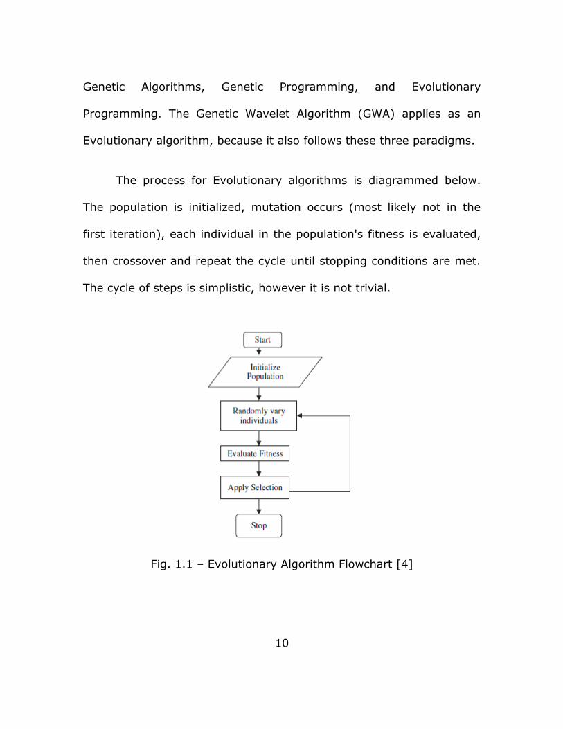
The process for Evolutionary algorithms is diagrammed below.

The population is initialized, mutation occurs (most likely not in the

first iteration), each individual in the population's fitness is evaluated,

then crossover and repeat the cycle until stopping conditions are met.

The cycle of steps is simplistic, however it is not trivial.

Fig. 1.1 – Evolutionary Algorithm Flowchart [4]

10

1.3 EA Uses and Limitations

There are many questions a developer should ask when

implementing an EA; for instance: how should one represent the

individuals of the population? What should the population size be? How

should the population be updated after selection is applied? How

should mutation affect an individual? When should the algorithm stop?

The answers to these questions is different for certain type of EAs, and

is also dependent on the type of problem being solved.

Before addressing the above questions concerning

implementation details of EAs, there is a simpler question that needs

to be answered: Why Evolutionary Algorithms? EAs are essentially a

form of search. So, what sets it apart from other approaches when

considering how to solve a problem? Some advantages include:

"simplicity of approach, its robust response to changing circumstances,

and its flexibility."[4] Holland argued that the power of EAs (more

specifically GAs) comes from their ability to solve problems in an

"implicitly parallel fashion."[16] Part of the flexibility of EAs is the wide

variety of problems that can be solved. If a problem can be formulated

as a functional optimization problem, then it can be solved by EAs. In

addition, EAs have the ability to solve problems that have not been

11

solved. "Fogel (1995) declaired artificial intelligence as 'They solve

problems, but they do not solve the problem of how to solve

problems.' In contrast, evolutionary computation provides a method

for solving the problem of how to solve problems."[4]

EAs are not the answer to every problem, because they have

some problems of their own. Some optimization problems lead EAs to

false solutions, when the algorithm finds a locally optimal solution that

meets the stopping criteria. Locally optimal solutions represent roots

(local maximum or minimum points in the search space), and to an

EA, "one root is as good as another."[5] Highly nonlinear functions are

also difficult for EAs to optimize, partly due to a greater occurrence of

locally optimal solutions. "Typical approaches to highly nonlinear

problems involve either linearizing the problem in a very confined

region or restricting the optimization to a small region. In short, we

cheat."[5] Another limiting factor of EAs is the representation of an

individual's genome. For example, If it is chosen to be a fixed length,

then that is a limiting factor for the solution - if the optimum solution

does not fall within the representation's range of solutions, then the

optimal solution will not be found. Another disadvantage of EAs is

setting one up to solve a problem. A great amount of understanding of

12

a problem is required to know how to represent a solution, tests its

fitness and have an effective termination condition.[10]

This paper approaches the topic of Evolutionary Algorithms first

by providing an understanding of existing genetic algorithms and then

relating the paradigms found in GAs to the formal definition of the

Genetic Wavelet Algorithm.

13

2. Classic Genetic Algorithms

“An algorithm is a series of steps for solving a problem. A

genetic algorithm is a problem solving method that uses genetics as its

model of problem solving."[4]

2.1 Introduction to the Classic GA

Genetic Algorithms (GAs) are a common example of evolutionary

algorithms. There are many different variations of GAs. A classic or

simple GA represents the solution with a fixed length string, usually a

bit string. GAs use recombination and mutation to generate the next

iteration of a population. "The objective function or fitness function

f(s) plays the role of the environment; each individual s is evaluated

according to its fitness. In this way a new population (iteration t+1) is

formed by selection of the better individuals of the former population,

as they will form a new solution by means of applying selection

procedure and crossover and mutation operators. It should be noted

that diversity of individuals is required to find good solutions with

GA."[2] The steps of simple GA are outlined below.

14

Figure 2.1 – Genetic Algorithm Flowchart [5]

Above is a flowchart similar to the example given for EAs. In this

flow chart, the generic steps for EAs are expanded and detailed to

show the more specific process of a simple GA. The first step is the

initialization of the problem's fitness function, which is referred to as

cost in the flowchart because it applies to a minimization problem. An

initial population is generated (usually randomly). Next, the algorithm

simulates generations of individuals by using the genetic operators

(crossover and mutation) until the stopping criteria is met.[5] The

logical steps for GAs are a little less simplistic than in EAs and are not

defined well enough in the diagram above.

15

Before the algorithm can start, the encoding of the chromosome

has to be chosen. The encoding will be a fixed length string, therefore

any possible solution to the problem has to be able to be encoded in

the chromosome. That means that the scope of the problem (or at

least the desired solution space) has to be defined, and the

chromosome has to have the capacity to represent it.[4]

Next, the fitness function is defined. The fitness function needs

to enforce all the constraints and objectives of the problem. Any

constraint or objective "can be handled as weighted components of the

fitness function."[4] Therefore, if a particular individual violates a

constraint then the fitness value should decrease, and if it satisfies an

objective then the fitness value should increase. The amount of

increase/decrease is dependent on the weight of the constraint or

objective. The weight signifies the importance of each constraint

relative to another constraint.

After the parameters (encoding and the fitness function) of the

GA are set up, an initial population is created. The population size

should be large enough to ensure diversity amongst individuals, and is

also dependent on the nature of the problem. An initial population with

the greatest diversity amongst individuals is most beneficial for

16

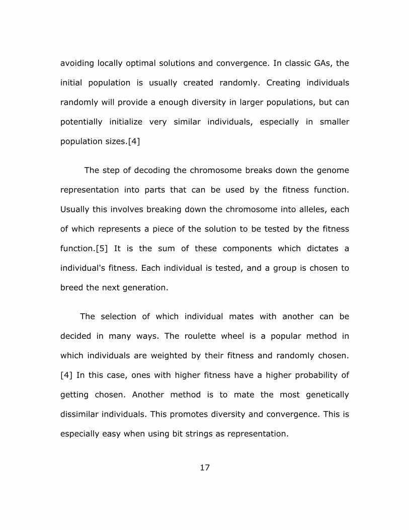
avoiding locally optimal solutions and convergence. In classic GAs, the

initial population is usually created randomly. Creating individuals

randomly will provide a enough diversity in larger populations, but can

potentially initialize very similar individuals, especially in smaller

population sizes.[4]

The step of decoding the chromosome breaks down the genome

representation into parts that can be used by the fitness function.

Usually this involves breaking down the chromosome into alleles, each

of which represents a piece of the solution to be tested by the fitness

function.[5] It is the sum of these components which dictates a

individual's fitness. Each individual is tested, and a group is chosen to

breed the next generation.

The selection of which individual mates with another can be

decided in many ways. The roulette wheel is a popular method in

which individuals are weighted by their fitness and randomly chosen.

[4] In this case, ones with higher fitness have a higher probability of

getting chosen. Another method is to mate the most genetically

dissimilar individuals. This promotes diversity and convergence. This is

especially easy when using bit strings as representation.

17

2.2 Mating and Crossover

Mating is the step of a GA in which the cross over operator is

applied to the selected mates to form a new individual. This step is

essentially concatenating substrings - one from each mate, the point

at which the string is split is called the crossover point. The placement

of the crossover point is dependent on how alleles are represented in

the chromosome string[4]. Taking parts from each parents string

representation and putting them together creates a new individual, but

how should these new individuals be put into the population? The new

generation could replace the old one completely, or some of the best

performing individuals could be kept in the population with the new

generation. Poor performing individuals should be removed from the

population. If the older generation is entirely replaced by the new one,

the algorithm runs the risk of backward progress (the new generation

performing worse than the old one). Below is an example of crossover,

bit strings a and b combine to create the two bit strings c and d.

Notice that this is very unlike the way genetic information is passed to

offspring in the biological context.

18

Fig. 2.2 – Crossover example [10]

Every GA has a mutation factor or mutation rate, which is just a

number that represents how large of a portion of the genome is

mutated for each individual. When mutation occurs, an individual

becomes more or less fit. The higher the mutation factor is, the less

powerful the crossover step is. However, if the mutation factor is low

(e.g. 1 bit in a bit string of length 1,000,000,000) then the population

will take more generations to generate diversity that does not already

exist in the population.[10] Mutation affects the chromosome

randomly; how it is applied is dependent upon how the genome is

represented. For instance when using a bit string encoding, bits are

flipped, but when using integers or real values mutation takes the

form of addition or subtraction.

19

The steps of evaluation, recombination and mutation are

performed until some stopping criteria is met. In genetic algorithms

the stopping criteria is convergence, meaning that the population has

converged towards a single solution or solution set.[4] Sometimes the

problem is such that if an individual reaches a certain fitness, the

answer is found. Convergence is measured by the most fit individuals

in consecutive generations. If the most fit individual is not improving

over many consecutive generations, then the algorithm has come to a

point of convergence. Convergence does not mean that the solution

has been found, but that a solution has been found. The solution could

be found to be locally optimal, in which case another constraint would

need to be added to the fitness function.

How does one encode diversity into these algorithms? Not

diversity amongst its population's individuals' chromosomes, but the

diversity that can be found by comparing a flea to a blue whale. It is

not easy, GAs chromosome representation is inherently discrete,

because they are fixed length strings. Fixed length means a predefined

minimum and maximum, making the scope of the individuals limited -

falling short of mimicking biological evolution's ability to adapt new

unseen traits in response to an environment.

20

21

3. Chromosome Representation for GAs

3.1 Importance of representation

"The coding of the variables in[binary] string structures make

the search space discrete for GA search. Therefore, in solving a

continuous search space problem, GAs transform the problem into a

discrete programming problem. Although the optimal solutions of the

original continuous search space problem and the derived discrete

search space problem may be marginally different (with large string

lengths), the obtained solutions are usually acceptable in most

practical search and optimization problems. Moreover since GAs work

with a discrete search space they can be conveniently used to solve

discrete programming problems, which are usually difficult to solve

using traditional methods." GAs are diverse and capable of solving

difficult problems that non-evolutionary search algorithms have

difficulty solving. Encoding the solution in bit strings has its limits. This

limit has been recognized by computer scientists, and other techniques

of representation have been developed for removing some of these

limitations.

22

The way a GA represents an individual's chromosome is

important for understanding its limitations and application to classes of

problems. On some level, any chromosome is represented by a bit

string, because that is how the computer understands it; however,

what is important is how alleles are represented, because they are the

smallest logical element of a chromosome in GAs.

3.2 Approaches to chromosome representation

Heinz Muhlenbein says that GAs can be broken down into three

general approaches to chromosome representation: phenotypic,

genotypic, and statistical.[2] Phenotypical approach is more concerned

with the actual observable behavior of an object than its specific

genes. An example of a phenotype would be the color of someone's

eye - there are many genes that go into affecting this, but it is

observed as a single characteristic. Phenotypic approaches correlate

the chromosome representation directly with a phenotype, instead of

using genotype to phenotype mapping. An example of this could be a

bit string, in which each bit corresponds to whether or not the

individual possesses a specific trait. One benefit of this is for

abstracting more advanced behavior in individuals, however it is

further away from the capabilities of genetic representation found in

23

nature.

"If a phenotypic property of an individual, like its hair color or

eye size is determined by one or more alleles, then these alleles

together are denoted to be a gene. A gene is a region on a

chromosome that must be interpreted together and which is

responsible for a specific phenotypic property."[3] The genotypic

approach is almost directly opposite of the phenotypic approach. In

genotypic chromosome representation, the bit string corresponds to an

individuals exact genetic makeup. The genotypic approach requires a

genotype to phenotype map, which takes a substring of the genome

(representing an allele) and maps it to an observable phenotype. This

is a representation more accurate to what actually happens in

biology; a being's phenotypes are influenced by its genotype and the

environment. Many components of a being's genotype may make up

one visible phenotype. In biology, these components are not usually

contiguous, but are dispersed about the genome; however in GAs, the

substring is usually contiguous.

The statistical approach, unlike the others, takes into

consideration the whole chromosome of each of the individual's

24

parents. For each allele in each parents' chromosome representation,

the gene that the offspring will have is determined statistically

depending on the values of the alleles. This could be implemented as

some alleles being dominant or recessive, or the resulting could be a

combination of both alleles - it all depends on the problem being

implemented.

3.3 Types of Representations

Below is a table summarizing common representation types for

chromosome encoding in GAs. Gray coding and unary coding are

mentioned in reference to binary strings and are explained below the

table.

25

Fig. 3.1 – Table of chromosome representation.

26

Sometimes a problem occurs when using binary strings in GA

optimization problems: the "Hamming Cliff." The Hamming Cliff

problem occurs when two parents have bit strings that are dissimilar,

but close in value.[1] Take the bit strings "10000000" and

"01111111", their decimal values are 128 and 127 respectively, which

is one digit away. However, their bit strings share no common values.

A real world example of this would be if there were two nearly identical

people standing next to each other that didn't have any shared DNA. It

would not be a problem if it weren't for the offspring these strings

would produce. For instance, say that the crossover point were to be

after the third digit. Parents with those bit strings would produce

offspring that were represented by the bit strings "10011111" and

"01100000." The decimal value of these strings are 159 and 96

respectively. The parents are well fit individuals – we assume this

because they are chosen to be mated; because their values are close,

it can also be assumed that they are near a point of convergence. The

resulting offspring have decimal values very far from their parents,

therefore delaying convergence. One solution to the Hamming Cliff

problem is to use gray coding for bit strings. Gray coding ensures that

consecutive numbers have at most one different bit. With gray coding,

the same parents could be represented by the bit

27

strings "11000000"(128) and "01000000"(127). With the same

crossover point, they would produce two offspring identical to

themselves.[5]

Another solution to the hamming cliff problem is unary coding.

Unary coding is a simple alternative to standard bit strings; an integer

n is represented by a bit string with n 1's followed by a 0. The length

of a unary coded string is directly related to decimal value of what it

represents. Therefore the number three would be represented by the

bit string "1110". This might not work well with a fixed length string,

because every bit string would have to be as long as the highest value.

A Schema is a way of representing potential individuals that use

bit string chromosome representation. Schemata are strings that

consist of 1, 0 and a wild card character. Take for example the schema

"1**10*1", "*" is the wild card character in this instance. The number

of non wildcard characters in the dictates the order of the schemata,

for the example given the order would be four. A powerful part of of

GAs is the ability to predict the number of copies of a particular

schema in the next generation of a population. After many

generations, well fit schemata that have been prevalent throughout

many generations are deemed as building blocks. After identifying

28

these building blocks, the schemata can be combined through

crossover to get a more fit schemata. Lower order schemata are more

likely to have high fitness, so the building blocks start out small, but

with the use of recombination they create larger building blocks which

speed up convergence.[4]

Variable length representation is not used in classical GAs.

Sometimes variable length encoding is useful for certain problem

representations. For example, if the problem solution were to be an

unweighted graph that is represented by an adjacency matrix. A

variable length solution would represent a graph with any number of

nodes and their edges. But how would one go about recombining these

adjacency lists so that they create valid structures and even if they do

create valid structures, are they closer to a convergence point? One

way could be to ignore invalid structures and let competition weed

them out. This strategy works as long as the fitness function has a

relatively few number of constraints to test, but if there are many

highly coupled constraints the existence of invalid children just works

to slow the algorithm down. Richard Dawkins thought of a different

way of representing complex problems in GAs - biomorphs. "Taking its

inspiration from nature, this approach focuses on genotypic

29

representations that represent the plans for building complex

phenotypic structures through a process of morphogenesis."[7] In his

book - The Blind Watchmaker - Dawkins describes "biomorphs" as a

way of representing the behavior of a complex object (instead of the

object itself). Genes dictate some sort of behavior, like development,

instead of traits like height. Instead, the height of an object would be

determined by the gene that controlled development.[17]

30

4. Other Types of Genetic Algorithms

4.1 Adaptive Genetic Algorithms

Adaptive Genetic Algorithms (AGA) are GAs that adapt their

parameters while running. Such parameters may include population

size, crossover probability or mutation probability. The algorithm is

responsive to how much the population improves, for instance if it is

not improving much, then the mutation rate may go up.[4] The flow

chart for this would look almost identical to that of the GA, with the

addition of one step - applying the heuristic for regulating the GA

parameters. This happens after the population is evaluated, at the end

of the GA loop.

By evolving the parameters that are kept constant in traditional

GAs, AGAs are trying to overcome some of the problems inherent to

GAs. The first of which is locally optimal solutions. If the GA is

converging upon a locally optimal solution, the growth rate of

population fitness starts to approach zero. When this happens, the GA

will adapt by increasing the mutation factor. This will increase diversity

in the next generation, which will provide the GA with new individuals

that are not stuck on local optima.

31

4.2 Fast Messy Genetic Algorithms

Fast Messy Genetic Algorithms (fmGA) is a type of GA that uses

variable length binary strings as encoding. The principal feature of

fmGAs is their use of building blocks "to explicitly manipulate building

blocks (BBs) of genetic material in order to obtain good solutions and

potentially the global optimum."[4] The fmGA has three stages:

initialization, a building block filter phase, and the juxtaposition phase.

The parameter of the length of the building blocks is given to

compensate for the variable length strings. Initialization starts with a

population sizing equation that finds a size large enough to overcome

the noise caused by the building block filtering phase. Once population

size is established, a population is randomly generated and their

fitness is evaluated. Members of the population are then used to

derive a building block that is the desired length. This is accomplished

by a building block filtering schedule, which constitutes the building

block filtering phase. In this phase, a certain number of bits are

randomly deleted from each member of the population. This removal

of bits is alternated with a tournament-style selection so that only the

fittest building blocks get selected. The building block filter phase is

completed when every member of the population has the same length

as specified in the problem parameters. In the next phase, the 32

juxtaposition phase, the best building blocks are randomly chosen and

cross over is applied - the crossover point is chosen based upon a

probability distribution. This step creates individuals whose strings

may or may not be larger than the specified building block size, these

individuals make up the next generation. These phases are repeated

until convergence or finishing criteria are met.[4]

4.3 Independent Sampling Genetic Algorithm

Another variation on the classic genetic algorithm is the

Independent Sampling Genetic Algorithm (ISGA). The ISGA has two

phases: the independent sampling phase and the breeding phase. "In

the independent sampling phase, a core scheme, called Building Block

Detecting Strategy (BBDS), to extract relevant building block

information of a fitness landscape is designed. In this way, an

individual is able to sequentially construct more highly fit partial

solutions."[4] The breeding phase employs a similar technique to one

described previously in this paper. Essentially the individuals choose

their mates. This is done by finding a mate with a similar fitness that is

genetically dissimilar from itself. This algorithm uses a population and

a fitness function, but only for the purpose of extracting building

blocks. These building blocks are combined using an effective strategy

33

for convergence. This algorithm is powerful for problems with "difficult

landscapes."[4] This means that problems that have many local

optima, will be overcome by the breeding of dissimilar pairs; it

promotes diversity.

34

5. Genetic Programming

5.1 Background

Genetic Programming (GP) is a specific application of GAs.

Instead of a bit string being evolved, a computer program is evolved.

It is evolved using the operators: mutation, crossover, and

"architecture-altering operations patterned after gene duplication and

gene deletion in nature."[4] GP was first introduced by John Koza in

his book, Genetic Programming: On the Programming of Computers by

Means of Natural Selection, published in 1992. GP stems from and is

similar to GAs, however has some important differences. Instead of

evolving bit strings, GP evolves tree structures that represent a natural

grammar parsing of the program's source code. In addition, GAs use

fixed length Strings, while GP needs to use trees which have variable

lengths. Instead of the search space being defined by the fitness

function, GP always searches for a solution in program space, or the

set of all programs that can be written by a language's formal

grammar. There is no formal logic required in the search, and there

35

does not need to be an explicit knowledge base in order to find a

solution. In addition, there is not a risk of converging onto a local

maximum. But how exactly does GP work?

5.2 Genetic Programming Process

It starts by initializing a population of tree structures. The tree

structures in GP are organized such that all leafs are terminals (values

or variables) and internal nodes represent functions. GP is

implemented with a maximum tree height to ensure that programs do

not become overly complex. There are two different methods for

initializing trees, "called full and grow."[18] Grow starts with a function

node at its root, and grows it by a single random node - terminal or

function - until all the leaves are terminals. Full generates only random

functions until the next node to be generated is at the maximum

height, then it generates random terminals. This results in a tree that

is full size.[18] Combining these two forms of tree creation provides an

initial population of many different sizes.

After the population is created, individuals are evaluated and

used for the creation of the next generation of programs. One

difference between GP and GAs is that GP keeps some inferior

programs, due to the possibilty that these programs could evolve into 36

a more optimal solution. Because GP keeps a population, these inferior

programs do not interfere with better performing ones. GP performs

crossover similarly to the way GAs do, by using a crossover point.

Instead of a place in a string, this is usually an edge in the tree. Two

parents produce two offspring, each of which contain complementary

parts of the parents. The process is diagrammed below, A and B are

the parents that crossover to create children C and D.

37

Fig. 5.1 – Genetic programming crossover example.

Evaluating the programs created by the process of GP can be

difficult. An implementation of GP needs to have a fitness function that

is able to distinguish between the hopeful solutions and the ones that

need to be weeded out. Programs may be generated that cannot be

compiled. "We can think of this as a form of infant mortality, in the

sense that programs that are not able to be successfully compiled

never get a chance to be executed."[7] Along with programs that are

not executable, some programs will have parts of their code that do

nothing to promote their fitness. "This phenomenon has been dubbed

'bloat' in the evolutionary computation community and appears to

have rather similar features to biological systems."[7] Bloat in

individuals has its own purpose - the bloat part could be modified

through crossover or mutation, and become something that makes the

individual more fit without affecting the parts that made it fit in the

first place.

The end conditions are met when the program produces a

certain output or when a convergence point has been found. In a

properly configured GP set up, convergence means that GP either

found the answer to the problem, or that the problem cannot be

38

solved with that maximum length program. The important part of GP is

evolving a set of instructions. Biomorphs had a similar theme in its

implementation.

39

6. Evaluation of Evolutionary Algorithms

When evaluating any type of EA, specifically GAs, it is necessary

to judge the problem which the algorithm is attempting to solve.

"when using specific representations some problems become easier,

whereas other problems become more difficult to solve for[Genetic

Evolutionary Algorithms]."[3] Therefore evaluation should start with

judging the problem. If the EA is using a different representation than

the easiest representation for the problem, then it is a sign to change

the chromosome representation. A few widely used methods for

measuring problem difficulty in GAs/EAs are correlation analysis,

polynomial decomposition, Walsh coefficients and schemata analysis.

[3]

Evaluating a solution is extremely important when dealing with

GAs, because of their tendency to find local extrema. Any solution

returned from a genetic algorithm should be recorded and written back

into the system for further generation. It is important to change the

parameters of the GA, such as population size and mutation rate,

when putting a found solution back into the GA.[4] In addition, GAs

use “metaheuristics” which essentially means that a single GA can

generate different solutions for separate runs. “This particular

40

characteristic of metaheuristics supposes an important problem for the

researchers when evaluating the results and, therefore, when

comparing their algorithms to other existing ones.”[11]

Comparing similar Genetic or Evolutionary algorithms is not an

easy task, and therefore often comes down to an empirical analysis of

one algorithms performance compared to another one. These

performances are tested over multiple well known problems. The

comparison consists of the quality of answer found and the

computational effort that is used to find the solution.

The most important part of evaluating the GWA is empirically -

by testing it against implementations of some of the algorithms

defined above. By comparing convergence on a range of difficult

problems, it will be clear if the complexity that the GWA introduces to

the classic GA creates a stronger Evolutionary Algorithm.

41

7. The Genetic Wavelet Algorithm

7.1 Introduction to the GWA

This paper has broadly covered the topics of EAs, GAs and GP.

The Genetic Wavelet Algorithm(GWA) has common characteristics with

these topics and the foundational information already presented is

important in order to understand the components of the GWA. The

GWA has a population of individuals that are evaluated by a fitness

function, and it uses recombination operators to create new

generations of the population, therefore it can be classified as an

evolutionary algorithm. However, there are more details that go into

the GWA than classic GAs. Below is a flow chart with the basic steps of

the GWA.

42

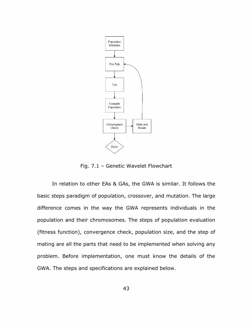
Fig. 7.1 – Genetic Wavelet Flowchart

In relation to other EAs & GAs, the GWA is similar. It follows the

basic steps paradigm of population, crossover, and mutation. The large

difference comes in the way the GWA represents individuals in the

population and their chromosomes. The steps of population evaluation

(fitness function), convergence check, population size, and the step of

mating are all the parts that need to be implemented when solving any

problem. Before implementation, one must know the details of the

GWA. The steps and specifications are explained below.

43

7.2 Population Initialization

Individuals in the GWA are represented as organisms. An

organism is made up of one or more cells. A cell has a nucleus which

contains one or more chromosomes. There can be single-cellular

implementations of the GWA or multi-cellular. An example of a multi-

cellular implementation would be a neural network.

The implementation of the organism is dependent on the

problem and how the programmer wants the genes to be represented

in the algorithm. This includes whether it is going to be a single-

cellular or a multi-cellular implementation. This organism also is where

genes would be mapped to traits.

Regardless of how an individual is implemented, a cell is initiated

the same way. A cell starts off with one chromosome, and a mutability

factor, a floating point variable between zero and ten. A cell can have

more chromosomes if mutation occurs; when it is instantiated, a

random number(between zero and ten) is tested against its mutation

factor, if the random number is less than the mutation factor, another

chromosome is added. This continues until a random number greater

than the mutability factor is chosen.

44

The GWA represents chromosomes as pairs of chromatids. Each

chromatid has a set of genes. There is a right chromatid and a left

chromatid. They are joined at what is called the centromere position,

which dictates where the gene will be split for crossover. Each

chromatid is instantiated with its own mutability factor, and then one

or more gene is added to the chromatid, depending on the same

method above for adding chromosomes to the cell.

The chromosome representation is done as objects in lists,

therefore an allele is not dependent on a position in a string, but on an

index in a list. At each index of the list is a gene object. There are

three types of genes: promoter genes, signal genes, and external

signal genes. Each gene has a list containing zero or more receptors.

Each gene has an output which is computed by its expression function.

This output is a floating point value and is essentially its value,

however the output of can also be represented by a set of wavelets,

more on this further on. Before additional detail on the types of genes,

it is important to discuss the concept of “key.”

The GWA uses keys, which use schemata to encode their values.

A key is a variable length string that is evolved during the genetic

45

wavelet algorithm using x as a wild card character. A key might look

like this:

Genetic Wavelets Signal Key Example: 01x01x10

A key is a schema, but it is not used for chromosome

representation, instead it is used to model communications between

cells in the GWA. Keys are used to represent two important

components of the GWA - receptors and signals. The interaction is

loosely modeled after hormones binding to cells. There are restrictions

for signals binding to receptors. A signal can bind to a receptor if and

only if the receptor matches the signal on all non-x points. For

example, the signal key "01101x10" can bind to the receptor

"110xx10," but "0101xx1" cannot bind to the same receptor.

46

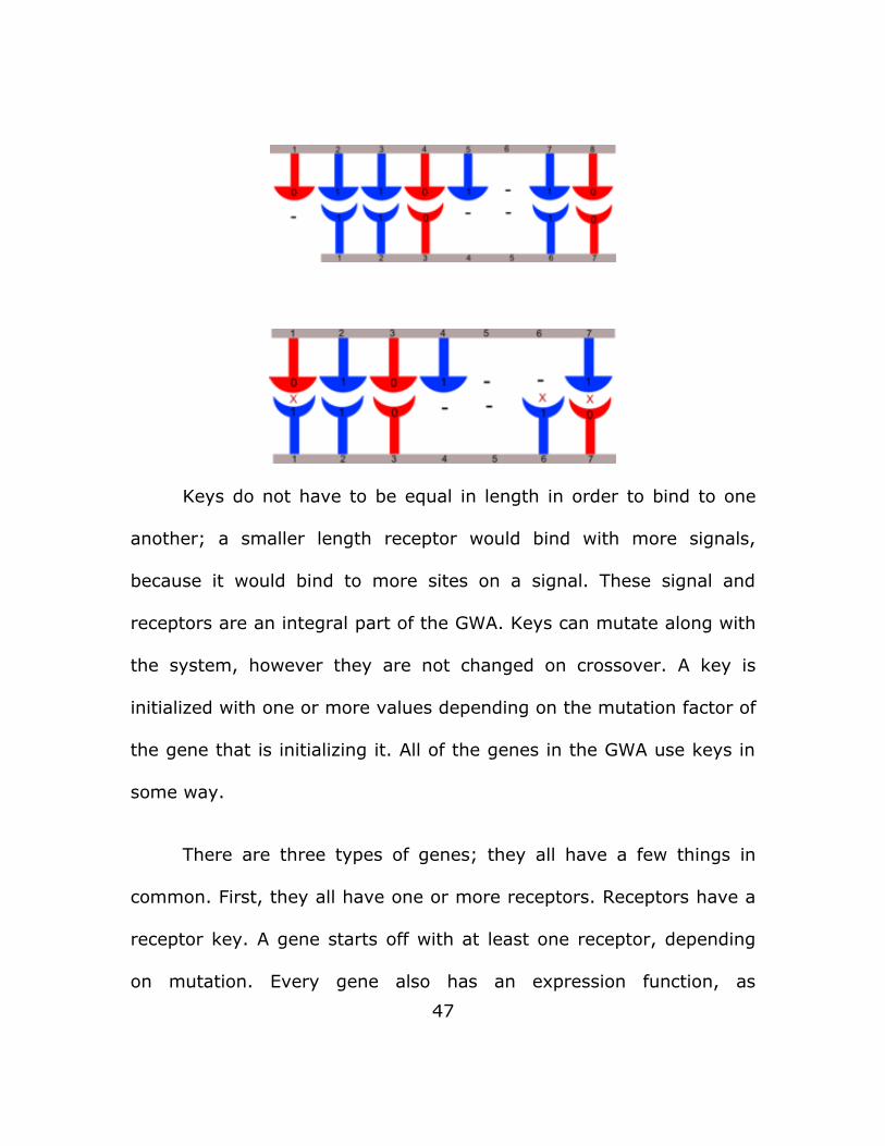
Keys do not have to be equal in length in order to bind to one

another; a smaller length receptor would bind with more signals,

because it would bind to more sites on a signal. These signal and

receptors are an integral part of the GWA. Keys can mutate along with

the system, however they are not changed on crossover. A key is

initialized with one or more values depending on the mutation factor of

the gene that is initializing it. All of the genes in the GWA use keys in

some way.

There are three types of genes; they all have a few things in

common. First, they all have one or more receptors. Receptors have a

receptor key. A gene starts off with at least one receptor, depending

on mutation. Every gene also has an expression function, as

47

mentioned before. The expression function is calculated using the

receptors to map each one to a dimension in a wavelet. More details

on how the expression function is calculated can be found in section

7.3. The floating point value output of the expression function is

known as the current activity of a gene – it is the value that it outputs.

The first type of gene is the signal gene. Signal genes are

responsible for creating a signal key that may or may not bind to other

genes' or its own receptors. Signals genes each have a concentration

which is calculated in the tick step. A signal gene outputs its signal

local to the cell it resides in. A signal binding to a receptor will increase

the output of that receptor by its concentration in the affected gene’s

expression function.

An external signal gene is similar to a signal gene, but it has a

direction that it is facing – it can either be inward facing or outward

facing. If it is outward facing, it outputs signals to other cells, and its

receptors receive signals from within the cell. If it is inward facing,

then it outputs signals to the local cell, and receives signals from other

external signal genes in other cells. These genes are only used in

multi-cellular implementations.

48

The final type of gene that is used in the GWA is a promoter

gene. Promoter genes exist to promote a gene that is a certain

distance away from it on the same chromatid. Promotion of a gene is

calculated and affects the current activity of a gene. The current

activity is increased by the product of its expression function output

and how much it is being promoted. The gene that a promoter gene

affects can change due to mutation.

The step of population initialization starts with filling the

population with randomly generated individuals. Each one of those

individuals is created with one or more cells, each containing one or

more chromosomes. Each chromosome is initialized with one or more

gene, which could be a signal, external signal, or promoter gene.

7.3 Pre-Tick, Tick, Wavelets, and the Expression Function

The pre-tick step is the first step in the simulation phase. This is

where each gene calculates its new activity from its expression

function. This is stored as its pending activity, because it is not applied

as its expression yet. Each signal that is being expressed in the cell is

tested to see if it binds to each receptor on the cell. If it does bind to a

cell, then its value is changed, if not its value is zero.

49

This step in the simulation calculates and applies the promotion

value. The current activity is set to the sum of the pending activity and

the product of the pending activity and its gene’s promotion.

Promotion does not affect value of the expression function, just

changes its output.

The expression function is the core of the GWA, and the origin of

the algorithm’s name. The expression function is a collection of one or

more wavelets. A wavelet is a wave that starts out with amplitude of

zero which increases and then goes back to zero. A common example

of a wavelet is the wave caused by a heartbeat. A wavelet is described

by a few different properties: amplitude, center point, phase, form,

and distribution. When a gene is initialized, the expression function is

created with one initial wavelet that is generated randomly. The

number of wavelets in the expression function is dictated by mutation.

When a gene mutates, its expression function has a chance to add,

remove, or modify wavelets. Below are two examples of what the

expression function could look like. The first is a two dimensional one

(two receptors) with one wavelet, the second one is what it would look

like if another random wavelet were to be added to it.

50

Fig. 7.2 – Wavelet examples

The expression function is multi-dimensional; each dimension

corresponds with a receptor, and the receptors value. A receptors

value is zero, unless a signal binds to it. Each wave in the expression

51

function will have the same dimensional values. So, in the above

examples you see each wave has two dimensions – x and y. Therefore

if these waves were expression functions, the genes that they were

from would only have two receptors on them. Or they could have

twenty receptors and only have two of them actually be bound to

signals.

The expression function can be used in two ways, through its

floating point output, and as a single function that it can represent.

Because the expression function is a function, it can be used as part of

the solution. For instance, by using a technique called convolution,

multiple wavelets can be combined into a single wavelet; using the

technique on the two wavelets above result in the wavelet below.

Fig. 7.3 – Wavelet transform example52

Using a gene’s expression function as a way to map the

organisms’ behavior depending on different input could yield powerful

results. Again, the way the genes affect an organism is up to the

details of the problem and its implementation. Either way, the

expression function’s method of adding multiple multi-dimensional

wavelets is an effective way of building a diverse function. The

algorithm can also be implemented by using the expression function’s

floating point output.

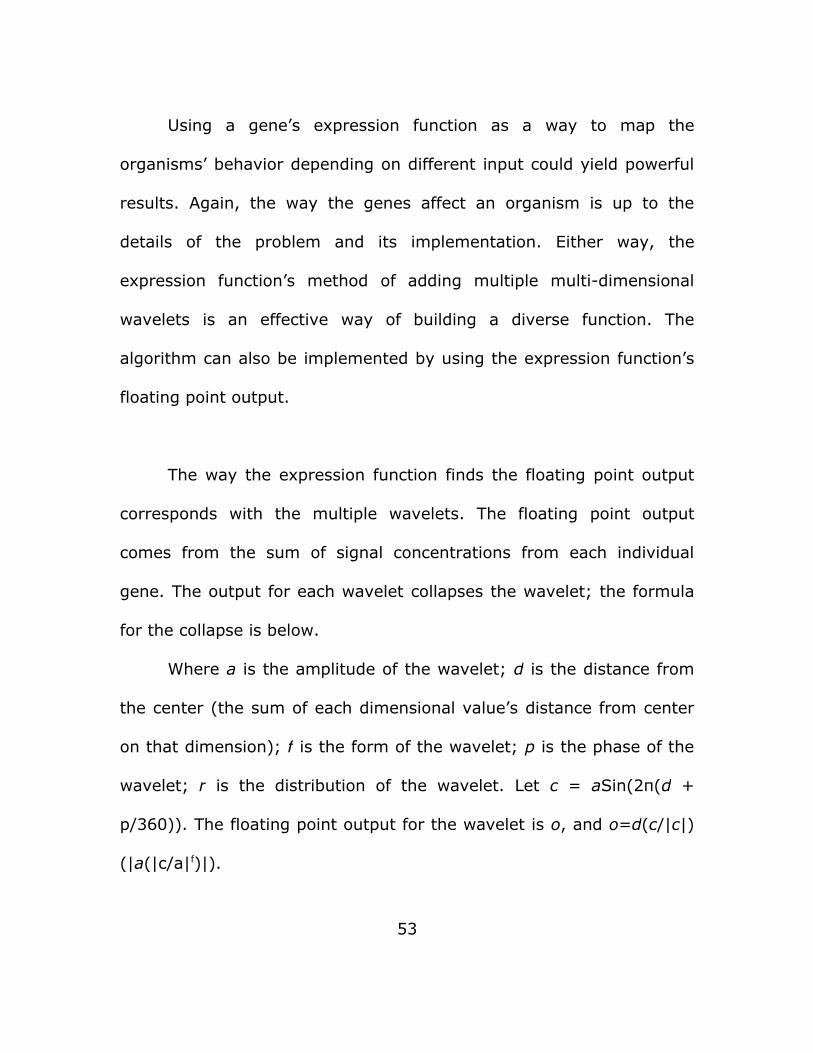
The way the expression function finds the floating point output

corresponds with the multiple wavelets. The floating point output

comes from the sum of signal concentrations from each individual

gene. The output for each wavelet collapses the wavelet; the formula

for the collapse is below.

Where a is the amplitude of the wavelet; d is the distance from

the center (the sum of each dimensional value’s distance from center

on that dimension); f is the form of the wavelet; p is the phase of the

wavelet; r is the distribution of the wavelet. Let c = aSin(2π(d +

p/360)). The floating point output for the wavelet is o, and o=d(c/|c|)

(|a(|c/a|f)|).

53

Whether using the floating point output or the wave function

output, the expression function is what is used to calculate the values

of each gene depending on the signals that exist in a cell, and the

receptors that those signals bind to. This process was modeled off of

Gene Regulatory Networks, which is the structure by which organisms

propagate their genes.

7.4 Evaluating the population and Convergence Check

The fitness function can be implemented like that in any other

GA, and it will differ greatly depending on the problem that is trying to

be solved. Each gene on the GWA has two potential outputs that could

be used in the fitness function as mentioned above. So it needs to be

decided whether the implementation is going to be dealing with graphs

or values. The evaluation step starts with going through each

individual, and evaluating them. Evaluation has to do with how well

their genes perform in the fitness function. These details are

dependent upon the problem being solved by the algorithm. The

convergence check is also dependent on the implementation;

traditional checks for convergence were outlined in previous chapters.

54

7.5 Mate and Mutate

Compilation is the process where two virtual organisms mate to

produce a new phenotype belonging to its child. This process is

modeled partly after Meiosis in biological organisms. First each parent

selects one chromatid from each chromosome at random to pass on to

the child. Next each sister chromatid from each parent, pair up at the

centromere to reform a chromosome as a composite from each parent.

In the end each child will have exactly half of its chromatid from each

parent. In addition, each child will have exactly the same number of

chromosomes as either parent. Through this process of compilation

new children organisms can be formed from mating parents.

Of course all this assumes no mutations occur. Due to mutation it is

possible for the chromosome count, chromatid count, and gene count

can all differ significantly. Since mutations are usually rare populations

should have time to normalize to ensure that such variation will be in

the minority.

The mating step is another item that needs to be implemented,

but it is not necessarily dependent upon the problem. The crossover

55

operator is already defined for chromosomes. What needs to be

defined is which individuals will mate with other individuals. When this

occurs, mutation in the genes is simulated using each chromatid’s

mutability factor. The number of chromosomes can also be mutated

based upon the mutation factor in each cell of the organism.

Which individuals get chosen for the next generation of the

population also needs to be decided by whoever is implementing the

algorithm. There are many methods of choosing this that have been

described in previous chapters, any of which could possibly be

implemented.

7.6 Evaluating the GWA

This algorithm was recently invented; therefore it has not been

critically compared against existing genetic algorithms. Therefore its

performance compared to other GAs on multiple different types of

problems must be empirically examined. The important things to

compare are: the number of generations it takes to converge, the

number of local optima found, and the evolvability of each algorithm.

Evolvability describes the ability of a genetic algorithm to come up

with complex novel solutions to a problem; this is best tested in a

56

problem with no solution, possibly something based on behavior in a

stochastic environment.

There are some parts of the GWA that could be evaluated by

other metrics. The first of which is its use of schemata – how does the

way the GWA use schemata relate to building blocks or the implicit

parallelism of schemata that Holland talked about? Also how does it

perform when the using the expression functions wavelet output to

solve problems that have very linear problem spaces? Are there things

that could be modified or improved with the current design? All these

questions are important for proving the validity, finding the strength,

and know the place of the Genetic Wavelet Algorithm.

57

8. Evaluation of the Genetic Wavelet

Algorithm

8.1 Introduction

Both empirical and theoretical evidence is needed in order to

accurately measure the GWA’s strength as a genetic algorithm. The

empirical test is comparative in nature, testing the GWA against a

simple genetic algorithm (sGA) with a fixed-length chromosome

representation and floating points as genes. In order for the empirical

data to be accurate, the algorithms need to be compared on a set of

problems with varying complexity and difficulty to solve.

8.2 Multiple Knapsack Problem

` The Multiple Knapsack Problem(MKP) is an optimization

problem; given n knapsacks of a certain capacity and k items each

item having a size and a cost, fill each knapsack to the greatest cost

58

per size by placing items in them without the sum of the sizes of the

items in a knapsack exceeding the capacity of the knapsack.

The MKP is in the class of problems called NP-hard[19] – which

are the hardest of the problems that take exponential time to find the

optimal solution. This is a good problem to be solved by Genetic

Algorithms, because it can be easily encoded into a chromosome, and

has a simple measure of success – how full the knapsacks are. The

combinatorial nature of this problem makes it difficult to find an

answer using traditional exhaustive search methods, especially as n

and k increase.

Genetic algorithms are not guaranteed to find an optimal

solution for every instance of the MKP. The comparison will be

between the solutions produced by the GWA and sGA on the same

instance of the MKP. The most fit individuals will be compared in

intervals of generations. The individuals that the algorithms converge

to and at which generation that individual was initially produced will

be compared. These metrics will show which algorithm gets a more

accurate solution faster and the diversity between generations.

It is important to understand what instances of MKP are

considered harder to solve than others. Testing on random sets of

evenly distributed data does not guarantee a hard problem. The

59

knapsack problem is considered to be one of the easier of the NP-hard

problems to approximate. There is a good measure of how hard an

instance of the problem will be. “The problems become harder as the

data range is increased.” [19] The data range is the distribution of the

item values. In problems where items are represented as integers,

the valid data range is the size of the largest knapsack. The difficulty

of the problem can also be determined by its ratio of number of items

and the data range, a value above 1000 is most likely going to be a

hard problem. [19] The larger the ratio, the harder the problem.

To compare the two algorithm implementation, the algorithms

are tested on many MKP instances with varying degrees of hardness,

where the item size to data range ratio is 100, 500, 1000, 2500, and

5000; Comparing the two algorithms on many problem instances at

those difficulty levels as well as once with a random distribution, will

provide reliable results that can be used to conclude the effectiveness

of the GWA on optimization problems compared to the sGA.

8.3 sGA Implementation of Multiple Knapsack Problem

Using the dANN Java AI framework, a simple genetic algorithm

using fixed length chromosomes was implemented. The length of the

60

chromosome is the same as the number of items in the instance of

the MKP that it is solving. The chromosomes use floating point values

as their genes. One gene represents one item in the list.

The fitness function orders the genes by their floating point

values. The function iterates over the ordered list of genes. The size of

the item that corresponds with each gene in the list is compared

against the remaining space of the current knapsack. If there is not

enough room to place the item in the knapsack, the function proceeds

to the next knapsack. If there are no more knapsacks, the function

ends. The fitness function calculates the weight of the knapsacks by

taking the sum of the product each item's size and cost/weight. The

cost/weight corresponds to item density, and will always be a double

value between 0 and 1(exclusive). The weight of the knapsacks is then

divided by the total space of the knapsack. This is also a double value

between 0 and 1(exclusive), that represents the weight per size of the

knapsack. This is a good measurement of fitness, because it

represents the value that needs to be optimized in the MKP.

61

8.4 GWA Implementation of Multiple Knapsack Problem

The current version of the GWA in the dANN library has

everything needed for initializing chromosomes and GWA individuals.

The population, individuals, mating, and the fitness function were all

implemented specifically for the MKP. The GWA, by default,

instantiates individuals with one chromosome with one gene on that

chromosome. There is a chance that a mutation event will occur and

there will be more genes or chromosomes added to that individual. In

order to fairly compare the GWA and sGA's performances, the fitness

functions should be the same. Because the sGA's fitness function

required a fixed length chromosome, and the GWA was implemented

to use a fixed length chromosome as well. This is to ensure that there

is not an advantage given to either algorithm in their respective fitness

functions.

The implementation of the GWA for MKP is constrained. There is

only one chromosome is allowed and it is fixed at the number of items

in the problem instance. The individuals are single cellular. The goal of

this comparison was to test whether or not the underlying mechanisms

involved with gene values are superior to the classic sGA. No new

signals will be introduced to an individual after it is initialized. The

62

problem has been constrained as such in order to ensure that the

results are such only due to that mechanism.

Mating was implemented as described in the section on mating

from the previous chapter. A chromatid was randomly selected from

the each of the two parents, combined, crossed over and possibly

mutated. After that the child is added to the population and tested.

There is also a chance that existing members of the population will

mutate on any given generation iteration.

8.5 Results and Comparison

A program was written called Genetic Algorithm Comparator

(GAC) to test the two genetic algorithms side by side on the same

problem instance. The problem was initiated with a hardness factor

described in section 8.2, and a random MKP of that hardness was

generated and tested. Both algorithms were run on many sets of

problems at different difficulty levels. Each algorithm was initialized

with a starting population of 50 individuals, a die off rate of 40%, and

a mutability of 20%. After the algorithms solve the same instance of

the MKP, their fitness functions are compared and the one with a

higher fitness value is considered to be more accurate. The ideal

63

solution is not calculated, the algorithms’ performances are instead

compared to each other. The results are below; each difficulty has two

bars, the first one represents the number of problems solved from that

particular hardness and each subset represents the number of

problems which one of the algorithms has a more accurate solution or

if their accuracy is equivalent. The second bar corresponds to the

problems which the algorithms were equally accurate, and is split up

into sections denoting the number of ties in which the particular

algorithm found the solution in less generations. The section labeled

TRUETIE refers to finding the solution in the same generation.

Fig 8.1 GWA sGA Comparison Results

64

100 100 500 500 1000 1000 2500 2500 5000 50000

50

100

150

200

250

300

TRUETIEGWATIESGATIETIEGWASGA

hardness

Num

ber o

f pro

blem

s

The results of comparison are clear, the sGA out performs the

GWA on all of the different problem difficulties in terms of getting a

more accurate solution. The problem instances in which each algorithm

finds the same solution are counted as a tie. The ties are attributed to

the algorithm that found the solution in the least amount of

generations. The graph below shows the percentage of problems that

were more accurately solved by each algorithm.

Fig. 8.2 – Graph representing percentage of problems that each

algorithm provided a superior solution for.

The GWA was less accurate than the sGA on 52% of the

problems tested. The sGA was less accurate than the GWA on 32% of

the problems tested. The two algorithms tied on 16% of the problems.

65

100 500 1000 2500 50000

0.1

0.2

0.3

0.4

0.5

0.6

0.7

SGAGWATIE

hardness (n/R)

%

A tie means the answer’s accuracy is the same, but a tie can be

broken by the number of generations that were needed to create that

individual. Below is a graph showing the percentages of ties that were

broken by the GWA or the sGA. If the two algorithms created the

individual on the same generation, then it was considered a true tie. If

the ties that were broken were attributed to each algorithm’s accuracy,

then the sGA would have been more accurate 54.8% of the time and

GWA would have been more accurate 42.72% of the time.

Fig 8.3 – Graph Showing Percentage of Resolvment of Ties

The sGA won 18% of the ties encountered in the data sets. The

GWA won 67% of its ties, and 16% were true ties. This data suggests

that the GWA converges more quickly upon solutions than the sGA. If 66

100 500 1000 2500 50000

0.1

0.2

0.3

0.4

0.5

0.6

0.7

0.8

0.9

SGATIEGWATIETRUETIE

hardness (n/R)

%

the GWA converges faster, then why is it not as accurate? The graph

below details the average offset of fitness values between the two

algorithms over all the problems.

Fig. 8.4 – Graph showing the average difference between the sGA and

GWA's winner fitness when each algorithm has a more accurate

solution than the other.

67

100 500 1000 2500 50000.00%

2.00%

4.00%

6.00%

8.00%

10.00%

12.00%

14.00%

16.00%

18.00%

%dif f SGA%dif f GWA

hardness

Aver

age

% s

uper

iorit

y

The difference in fittest individual fitness values shows how close

a winning individual's fitness was to a losing individual's fitness. For

the GWA, the average percent superiority for all levels of hardness is

less than 2%. This means when the GWA generates a more accurate

solution, it is on average less than 2% higher than the sGA's fitness.

On the other hand, when the GWA loses it loses badly. The drastic

difference in average fitness begs the question – why is the GWA being

outperformed so badly when it loses?

The large gap means that the GWA is getting stuck on local

optima. The restricted version of the GWA may be too constrained.

The fixed length chromosome had a negative effect on the GWA's

ability to diversify. In a non-constrained implementation the

chromosomes would be variable length; when a mutation occurred;

genes might be mutated, added, or removed from the chromosome. In

the fixed length implementation, genes are not added or removed,

only possibly mutated. In a population that is converging towards a

local optimum, the fitness values of the individuals and their genes will

be very similar. Without the ability to introduce new signals or

receptors to the gene pool the population has difficulty staying diverse.

Below is a chart demonstrating the average generation in which the

solution was found for each difficulty set.

68

Fig 8.5 – Chart demonstrating the average generation in which the

final solution was found for the different hardness levels of the MKP.

Despite the fact that the sGA outperformed the GWA on many

problem instances, some strengths of the GWA were apparent. The

GWA converges more quickly upon solutions compared to the sGA. In

the above graph, the average generation to find the solution in for the

GWA was approximately eleven. The average generation for the sGA

was almost thirty. Even when producing less accurate solutions, the

GWA converges upon its answer more quickly. The GWA won 67% of

ties, meaning if the sGA and GWA produced the same solution, on

average the GWA found the solution more quickly than the sGA. In

addition, the small average percentage of superiority of the GWA's

69

100 500 1000 2500 50000

5

10

15

20

25

30

35

Average SGA GenerationAverage GWA Generation

hardness

num

ber o

f gen

erat

ions

solutions shows that the sGA was very close to GWA's solution. The

fact that the GWA was only slightly more accurate also reinforces its

strength in converging on a solution. For fitness values that are very

close, the solutions that the individuals represent are similar. The GWA

was able to converge towards a more specific solution than the sGA,

exemplifying its ability to find a more specific answer than the sGA

without the sGA being stuck on a local optimum.

8.6 Conclusion

The constrained nature of this implementation of the GWA,

specifically the fixed length chromosome, causes the signals in an

individual to be less diverse. The lack of diversity causes this

implementation of the GWA to be susceptible to converging upon local

optima. When not tricked by local optima, the GWA performance

proved to be quick and reasonably accurate. The problem constraints

existed to test the random valued genes found in the sGA against the

weak links between genes caused by signal and receptor interaction

found in the GWA. The mechanisms dictating gene values in the GWA

are a valid and powerful technology unique to the field of Genetic

Algorithms. The code for this implementation is freely available at

http://github.com/koryk/GAC/.

70

Works Cited

[1] Bäck, Thomas; Fogel, David B.; Michalewics, Zbigniew. Handbook

of Evolutionary Computation. New York: Institute of Physics Pub.,

Oxford University Press, 1997.

[2] Winter, G. Genetic Algorithms in Engineering and Computer

Science. New York: Chichester, 1995.

[3] Rothlauf, Franz. Representations for Genetic and Evolutionary

Algorithms. New York: Springer, 2006.

[4] Mitchell, Melanie. An Introduction to Genetic Algorithms. Boston:

MIT Press, 1998.

[5] Hopt, Randy; Hopt, Sue. Practical Genetic Algorithms. Hoboken:

Wiley, 2004.

[6] Rutkowski, Leszek. Computational Intelligence: Methods and

Techniques. Berlin: Springer, 2005.

[7] De Jong, Kenneth. Evolutionary Computation: A Unified Approach.

Boston: MIT Press, 2006.

[8] Bentley, Peter; Corne, David. Creative Evolutionary Systems. San

Francisco: Kauffman, 2002.

[9] Higuchi, Tetsuya; Liu, Yong; Yao, Xin. Evolvable Hardware. New

71

York: Springer, 2006.

[10] Buckland, Mat. AI Techniques for Game Programming. Cincinatti:

Premier Press, 2002.

[11] Alba, Enrique; Dorronsoro, Bernabe. Cellular Genetic Algorithms.

New York: Springer, 2008.

[12] Riolo, Rick; O’Reilly, Una-May; McConaghy, Trent. Genetic

Programming Theory and Practice VII. New York: Springer, 2009.

[13] Gen, Mitsuo; Cheng, Runwei. Genetic Algorithms and Engineering

Optimization. New York: Wiley, 2000.

[14] Snustad, D. Peter., and Michael J. Simmons. Principles of

Genetics. New York, NY: John Wiley & Sons, 2003. Print.

[15] Darwin, Charles. Origin of Species. New York: Collier Press, 1909.

[16] “A Genetic Algorithm Tutorial.” Statistics and Computing. 4.2

(1994): 65-85.

[17] Dawkins, Richard. The Blind Watchmaker: Why The Evidence of

Evolution Reveals a Universe Without Design. New York: W. W. Norton

& Company, 1996.

[18] Banzhaf, Wolfgang. Genetic Programming - an Introduction: on

the Automatic Evolution of Computer Programs and Its Applications.

San Francisco: Morgan Kaufmann, 1998. Print.

72

[19] Pisinger, D. 2005. Where are the hard knapsack

problems?. Comput. Oper. Res. 32, 9 (Sep. 2005), 2271-2284.

73