Generic top-down discrimination for sorting and partitioning in … · 2015-07-07 · Generic...

JFP 22 (3): 300–374, 2012. c! Cambridge University Press 2012

doi:10.1017/S0956796812000160

300

Generic top-down discrimination forsorting and partitioning in linear time!

FRITZ HENGLEIN

Department of Computer Science, University of Copenhagen (DIKU), Copenhagen, Denmark(e-mail:)[email protected])

Abstract

We introduce the notion of discrimination as a generalization of both sorting and partition-ing, and show that discriminators (discrimination functions) can be defined generically, bystructural recursion on representations of ordering and equivalence relations. Discriminatorsimprove the asymptotic performance of generic comparison-based sorting and partitioning,and can be implemented not to expose more information than the underlying ordering,respectively equivalence relation. For a large class of order and equivalence representations,including all standard orders for regular recursive first-order types, the discriminators executein the worst-case linear time. The generic discriminators can be coded compactly using listcomprehensions, with order and equivalence representations specified using Generalized Al-gebraic Data Types. We give some examples of the uses of discriminators, including the most-significant digit lexicographic sorting, type isomorphism with an associative-commutativeoperator, and database joins. Source code of discriminators and their applications in Haskellis included. We argue that built-in primitive types, notably pointers (references), should comewith e!cient discriminators, not just equality tests, since they facilitate the construction ofdiscriminators for abstract types that are both highly e!cient and representation-independent.

1 Introduction

Sorting is the problem of rearranging an input sequence according to a given total

preorder.1 Partitioning is the problem of grouping elements of a sequence into

equivalence classes according to a given equivalence relation.

From a programming perspective, we are interested in not having to produce

hand-written code for each and every total preorder and equivalence relation one

may encounter but also to be able to do this generically: Specify a total preorder or

equivalence relation and automatically generate a sorting, respectively partitioning

function, that is both

• e!cient: it uses few computational resources, in particular it executes fast;

and

! This work has been partially supported by the Danish Research Council for Nature and Universe(FNU) under the grant Applications and Principles of Programming Languages (APPL), the DanishNational Advanced Technology Foundation under the grant 3rd generation Enterprise ResourcePlanning Systems (3gERP), and the Danish Council for Strategic Research under the grant FunctionalHigh-Performance Computing for Financial Information Technology (HIPERFIT).

1 A total preorder is a binary relation R that is transitive and total, but not necessarily antisymmetric.

Generic top-down discrimination 301

• representation independent: its result is independent of the particular run-time

representation of the input data.

E!ciency obviously seems to be a desirable property, but why should we be

concerned with representation independence? The general answer is, because “data”

are not always represented by the “same bits”, for either computational convenience

or for lack of canonical representation.

E!ciency and representation independence are seemingly at odds with each other.

To illustrate this, let us consider the problem of pointer discrimination: finding all the

duplicates in an input sequence of pointers; that is, partitioning the input according

to pointer equality. This is the problem at the heart of persisting (“pickling”) pointer

data structures onto disk, contracting groups of isomorphic terms with embedded

pointers, computing joins on data containing pointers, etc.

Let us try to solve pointer discrimination in ML.2 Pointers are modeled by

references in ML, which have allocation, updating, dereferencing, and equality

testing as the only operations. Representing references as machine addresses at

run time, the limited set of operations on ML references guarantees that program

execution is semantically deterministic in the presence of nondeterministic memory

allocation, and even in the presence of copying garbage collection. In this sense,

ML references are representation-independent: Their operations do not “leak” any

observable information about which particular machine addresses are used to

represent references at run time, giving heap allocator and garbage collector free

reign to allocate and move references anywhere in memory at any time, without the

risk of a"ecting program semantics.

Having only a binary equality test carries the severe disadvantage, however:

Partitioning a list of n references requires #(n2) equality tests, which follows from

the impossibility of deciding in sub-quadratic time whether a list of atoms contains

a duplicate.

Proposition 1Let T be a type with at least n distinct elements whose only operation is an equality

test. Deciding whether a list of n T -values contains a duplicate requires at least!n2

"

applications of the equality test in the worst case.

Proof(By adversary) Assume the problem can be solved using fewer than

!n2

"equality

tests. Consider input [v1, . . . , vn] with pairwise distinct input values v1, . . . , vn. Then

there is a pair vi, vj for some i, j with i "= j, for which no equality test is applied.

Change the input by replacing vi with vj . Now all equality tests performed for the

original input give the same result, yet the changed input has a duplicate, whereas

the original input does not. !

An alternative to ML references is to abandon all pretenses of guaranteeing

representation independence and leaving it in the hands of developers to achieve

whatever level of semantic determinacy is required. This is the solution chosen for

2 We use the term ML as a proxy for Standard ML, CaML, or any language in the ML family.

302 Fritz Henglein

object references in Java, which provides a hash function on references.3 Hashing

supports e!cient associative access to references. In particular, finding duplicate

references can be performed by hashing references into an array and processing the

references mapped to the same array bucket one bucket at a time. The price of

admitting hashing on references, however, is loss of lightweight implementation of

references and loss of representation independence: it complicates garbage collection

(e.g. hash values must be stored for copying garbage collectors) and makes execution

potentially nondeterministic. Computationally, in the worst case it does not even

provide an improvement: All references may get hashed to the same bucket. Pairwise

tests are subsequently necessary to determine whether they all are equal.

It looks like we have a choice between a rock and a hard place: Either

we can have highly abstract references that admit a simple, compact machine

address representation and guarantee deterministic semantics, but incur prohibitive

complexity of partitioning-style bulk operations (ML references), or we can give up

on light-weight references and entrust deterministic program semantics to the hands

of individual developers (Java references).

The problem of multiple run-time representations of the same semantic value

is not limited to references. Other examples are abstract types that do not have

an unchanging “best” run-time representation, such as sets and bags (multisets).

For example, it may be convenient to represent a set by any list containing its

elements, possibly repeatedly. The individual elements in a set may themselves have

multiple representations over time or at the same time; e.g. if they are references or

are themselves sets. The challenge is how to perform set discrimination e!ciently

so that the result does not leak information about particular lists and element

representations used to represent the sets in the input.

In this paper we show that execution e!ciency and representation independence

for generic sorting and partitioning can be achieved simultaneously. We introduce

a bulk operation called discrimination, which generalizes partitioning and sorting:

It partitions information associated with keys according to a specified equivalence,

respectively ordering relation on the keys. For ordering relations, it returns individual

partitions in ascending order.

As Proposition 1 and the corresponding combinatorial lower bound $(n log n)

(Knuth 1998, Sec. 5.3.1) for comparison-based sorting show, we cannot accomplish

e!cient generic partitioning and linear-time sorting by using black-box binary

comparison functions as specifications of equivalence or ordering relations. Instead,

we show how to construct e!cient discriminators by structural recursion on spec-

ifications defined compositionally in an expressive domain-specific language for

denoting equivalence and ordering relations.

Informally, generic top–down discrimination for ordering relations can be thought

of as filling the empty slot in the following diagram:

3 We use Java as a proxy for any language that allows interpreting a pointer as a sequence of bits, suchas C and C++; or provides a hashing-like mapping of references to integers, such as Java and C#.


Sorting Comparison-based Distributive

Fixed-order Quicksort, Mergesort, etc. with

inlined comparisons

Bucketsort, Counting sort,

Radixsort

Generic Comparison-parameterized

Quicksort, Mergesort, etc.

In particular, it extends distributive worst-case linear-time sorting algorithms to

all standard orders on all regular recursive first-order types, including tree data

structures.

The main benefit of generic discrimination is not for sorting, but for partitioning

on types that have no natural ordering relation, or where the ordering is not

necessary: It can reduce quadratic time partitioning based on equality testing to

linear time without leaking more information than pairwise equivalences in the

input.

1.1 Contributions

In this paper we develop the notion of discrimination as a combination of both

partitioning and sorting. Discrimination can be understood as a generalization of

binary equivalence testing and order comparisons from 2 to n arguments.

We claim the following as our contributions:

• An expressive language of order and equivalence representations denoting

ordering and equivalence relations, with a domain-theoretic semantics.

• Purely functional generic definitions of e!cient order and equivalence discrim-

inators.

• Representation independence without asymptotic loss of e!ciency: The result

of discrimination depends only on pairwise comparisons between keys, not

their particular values.

• A general theorem that shows that the discriminators execute in worst-case

linear time on fixed-width RAMs for a large class of order and equivalence

representations, including all standard orders and equivalences on regular

recursive first-order types.

• A novel value numbering technique for e!cient discrimination for bag and set

orders and for bag and set equivalences.

• Transparent implementation of generic discrimination in less than 100 lines of

Glasgow Haskell, employing list comprehensions and Generalized Algebraic

Data Types (GADTs), and with practical performance competitive with the

best comparison-based sorting methods in Haskell.

• Applications showing how worst-case linear-time algorithms for nontrivial

problems can be derived by applying a generic discriminator to a suitable

ordering or equivalence representation; specifically, generalized lexicographic

304 Fritz Henglein

sorting, type isomorphism with associative-commutative operators, and generic

equijoins.

• The conclusion that built-in ordered value types and types with equality,

specifically reference types, should come equipped with an order, respectively

equality discriminator to make their ordering relation, respectively equality,

e!ciently available.

This paper is based on Henglein (2008), though with all aspects reworked, and with

the following additional contributions: the domain theoretic model of ordering and

equivalence relations; the notion of rank and associated proof principle by structural

induction on ranks; the ordinal numbering technique for bag and set orders as

well as for bag and set equivalences; the explicit worst-case complexity analysis

yielding linear-time discriminators; the definition and semantics of equivalence

representations; the definition of generic equivalence discriminator disc (not to

be confused with the disc of Henglein (2008), which, here, is named sdisc); the

highly e!cient basic equivalence discriminator generator discNat; the definition,

discussion, and proof of representation independence; the application of equivalence

discrimination to type AC-isomorphism and database joins; the empirical run-time

performance evaluation and comparison with select sorting algorithms; the analysis

and dependency of comparison-based sorting on the complexity of comparisons;

and some minor other additions and removals.

1.2 Overview

After notational prerequisites (Section 2) we define basic notions: ordering and

equivalence relations (Section 3), and discrimination (Section 4).

Focusing first on ordering relations, we show how to construct new ordering

relations from old ones (Section 5) and how to represent these constructions as order

representations, potentially infinite tree data structures (Section 6). We then define

order discriminators by structural recursion over order representations (Section 7)

and analyze their computational complexity (Section 8).

Switching focus to equivalence relations, we show how to represent the com-

positional construction of equivalence relations (Section 9), analogous to the de-

velopment for ordering relations. This provides the basis for generic equivalence

discrimination (Section 10). We analyze the representation independence proper-

ties of discriminators (Section 11) before illustrating their use on a number of

paradigmatic applications (Section 12). We show that the practical performance of

our straightforwardly coded discriminators in Haskell is competitive with sorting

(Section 13) and discuss a number of aspects of discrimination (Section 14) before

o"ering conclusions as to what has been accomplished and what remains to be

done.

On first reading the reader may want to skip to Sections 6, 7, 12, and 13 to get

a sense of discrimination, its applications, and performance from a programming

point of view.


2 Prerequisites

2.1 Basic mathematical notions

Let R,Q # T $T be binary relations over a set T . We often use infix notation: xR y

means (x, y) % R. The inverse R&1 of R is defined by xR&1 y if and only if y R x. The

restriction R|S of R to a set S is defined as R|S = {(x, y) | (x, y) % R 'x % S ' y % S}.R $ Q is the pairwise extension of R and Q to pairs: (x1, x2)R $ Q (y1, y2) if and

only if x1 R y1 and x2 Qy2. Similarly, R( is the pointwise extension of R to lists:

x1 . . . xm R( y1 . . . yn if and only if m = n and xi R yi for all i = 1 . . . n. We write !x )=!y

if !y is a permutation of the sequence !x.

A (recursive) first-order type is a possibly infinite tree built from type constants

unit (1) and the integers Int; binary product ($) and sum (+) constructors; and the

unary foldT -constructor. Such a type is regular if it has only finitely many distinct

subtrees. A first-order type is inhabited by finite values generated by the grammar,

v ::= c | () | inl v | inr w | (v, v*) | fold (v)

where c % Int is an integer constant. In applications, other primitive types and value

constants may be added. A type scheme is a type where type variables are also

permitted. We denote the universe of all values by U.

The foldT -constructor is for interpreting recursive types iso-recursively: Its only

elements are values of the form fold (v). The notation µt.T [t], where T [t] is a type

scheme containing zero, one or more occurrences of type variable t, denotes the

type T * satisfying T * = foldT (T [T */t]). This mimicks Haskell’s way of defining

recursive types by way of newtype and data declarations. For example, the list type

constructor is defined as T ( = µt. 1 + T $ t, where we define [] = fold (inl ()) and

x :: !x = fold (inr (x,!x)) and use the notational convention [x1, . . . , xn] = x1 :: . . . ::

xn :: [].

Note that all lists and trees that can occur as keys are finite in this paper. For

emphasis, we note that types denote sets without any additional structure, such as

an element representing nontermination. We allow ourselves to use types also in

place of the sets of elements that inhabit them. (Only in Section 8 we treat types as

syntactic objects; otherwise they can be thought of as set denotations.)

We use Big-O notation in the following sense: Let f and g be functions from

some set S to !. We write f = O(g) if there are constants a, b % ! such that

f(x) ! a · g(x) + b for all x % S .

We assume basic knowledge of concepts, techniques, and results in domain theory,

algorithmics, and functional programming.

2.2 Haskell notation

To specify concepts and simultaneously provide an implementation for ready

experimentation, we use the functional core parts of Haskell (Peyton Jones, 2003)

as our programming language, extended with GADTs, as implemented in Glasgow

Haskell (Glasgow Haskell, 2005). GADTs provide a convenient type-safe framework

for shallow embedding of little languages (Bentley, 1986), which we use for a type-safe

306 Fritz Henglein

coding of ordering and equivalence representation as potentially infinite trees. Hudak

et al. (1999) provide a brief and gentle introduction to Haskell, but since we

deliberately do not use monads, type classes, or any other Haskell-specific language

constructs except for GADTs, we believe basic knowledge of functional programming

is su!cient for understanding the code we provide.

We are informal about the mapping from Haskell notation to its semantics. As a

general convention, we use fixed-width font identifiers for Haskell syntax and write

the identifier in italics for what is denoted by it. We use Haskell’s built-in types

and facilities for defining types, but emphasize that keys drawn from these types

here are assumed to belong to the inductive subset of their larger and coinductive

interpretation in Haskell. In particular, only finite-length lists can be keys here.

Haskell’s combination of compact syntax, support for functional composition, rich

type system, and comparatively e!cient implementation constitute what appears

to us to presently be the best available uniform framework for supporting the

semantic, algorithmic, programming, application, and empirical aspects of generic

discrimination developed in this paper. It should be emphasized, however, that this

paper is about generic discrimination, with Haskell in a support role. The paper

is not about Haskell in particular, nor is it about developing generic top–down

discrimination specifically for Haskell. We hope, however, that our work informs

future language and library designs, including the Haskell lineage.

2.3 Disclaimer

This paper emphasizes the compositional programming aspects of top–down generic

discrimination. It addresses semantic, algorithmic, empirical, and application aspects

in support of correctness, expressiveness, and computational e!ciency, but we avoid

detailed descriptions of mathematical concepts and only sketch proofs. A proper

formalization of the results claimed here in the sense of being worked out in

detail and, preferably, in machine-checkable form is not only outside the scope and

objective of this paper but is also what we consider a significant challenge left for

future work.

3 Ordering and equivalence relations

Before we can introduce discriminators, we need to define what exactly we mean by

ordering and equivalence relations.

3.1 Ordering relations

Definition 1 (Definition set)

The definition set def(R) of a binary relation R over S is defined as def(R) = {x %S | (x, x) % R}.

Definition 2 (Ordering relation)

A binary relation R # S $ S is an ordering relation over S if for all x, y, z % S:


1. ((x, y) % R ' (y, z) % R) + (x, z) % R (transitivity), and

2. ((x, x) % R , (y, y) % R) + ((x, y) % R , (y, x) % R) (conditional comparability).

Note that the condition for comparability is disjunctive: Only one of x, y must relate

to itself before it relates to every element in S . An alternative is replacing it by a

conjunction ((x, x) % R ' (y, y) % R). The present definition is stronger, and we use

it since it is noteworthy that the order constructions of Section 5 are closed under

this definition.

Not insisting on reflexivity in the definition of ordering relations is important for

being able to treat them as pointed directed complete partial orders (dcpos) below.

A word on nomenclature: An ordering relation is not necessarily antisymmetric,

so it is a kind of preorder, though not quite, since it is not necessarily reflexive on

all of S , only on a subset, the definition set. Analogous to the use of “partial” in

partial equivalence relations, we might call it a partial preorder. This would confuse

it with “partial order”, however, where “partial” is used in the sense of “not total”.

Note that conditional comparability implies totality on the definition set, and we

would end up with something called a partial total preorder, which is not attractive.

For this reason we just call our orders “ordering relations”. Formally, an order

is the pair consisting of a set and an ordering relation over that set; analogously

for equivalence. We informally use “order” and “equivalence” interchangeably with

ordering relation and equivalence relation, however.

For ordering relations we use the following notation:

x !R y - xR y

x "R y - y R x

x !R y ' y "!R x

x .R y - xR y ' y R x

x >R y - y <R x

x#R y - x "!R y ' y "!R x

Definition 3 (Domain of ordering relations over S)

The domain of ordering relations over S is the pair (Order(S),/) consisting of the

set Order(S) of all ordering relations over S , and the binary relation / defined by

R1 / R2 if and only if x <R1 y =+ x <R2 y and x .R1 y =+ x .R2 y for all x, y % S .

Proposition 2

(Order(S),/) is a pointed dcpo.

Proof

Let D be a directed set of ordering relations. Then the set-theoretic union#

D is

an ordering relation on S . Furthermore, it is the supremum of D. Observe that the

empty set is an ordering relation. It is the least element of Order(S) for any S . !

Note that / is a finer relation than set-theoretic containment: R1 / R2 =+ R1 #R2, but not necessarily conversely. For example, {(x1, x2)} # {(x1, x2), (x2, x1)}, but

{(x1, x2)} "/ {(x1, x2), (x2, x1)}. Intuitively, / disallows weakening a strict inequality

308 Fritz Henglein

x <R1 y to a nonstrict x !R2 y. This will turn out to be crucial for ensuring that the

lexicographic product order construction in Section 5 is monotonic.

3.2 Equivalence relations

Definition 4 (Equivalence relation)A binary relation E # S $ S is an equivalence relation over S if for all x, y, z % S:

1. ((x, y) % E ' (y, z) % E) + (x, z) % E (transitivity), and2. (x, y) % E + (y, x) % E (symmetry).

This is usually called a partial equivalence relation (PER), since reflexivity on S is

not required. Since a PER always induces an equivalence relation on its definition

set, we drop the “partial” and call all PERs simply equivalence relations.

We write x .E y if (x, y) % E and x ".E y if (x, y) "% E.

Definition 5 (Domain of equivalence relations over S)The domain of equivalence relations over S is the pair (Equiv (S),#) consisting of the

set Equiv (S) of all equivalence relations on S , together with subset containment #.

Proposition 3(Equiv (S),#) is a pointed dcpo.

ProofLet D be a directed set of equivalence relations. Then the set-theoretic union

#D

is an equivalence relation over S . Furthermore, it is the supremum of D. Observe

that the empty set is an equivalence relation. It is the least element for Equiv (S) for

any S . !

Each ordering relation canonically induces an equivalence relation:

Proposition 4Let R be an ordering relation. Then .R is the largest equivalence relation contained

in R.

4 Discrimination

Sorting, partitioning, and discrimination functions can be thought of as variations

of each other. The output of a sorting function permutes input keys according to a

given ordering relation. A partitioning function groups the input keys according to a

given equivalence relation. A discrimination function (discriminator) is a combination

of both, though with a twist: Its input are key-value pairs, but only the value

components are returned in the output.

Definition 6 (Values associated with key)Let !x = [(k1, v1), . . . , (kn, vn)]. Let R be an ordering or equivalence relation. Then the

values associated with k under R in !x is the list

vals!xR(k) = map snd (filter (pR(k)) !x)

where pR(k)(k*, v*) = (k .R k*).


Note that the values in vals!xR(k) are listed in the same order as they occur in !x.

Definition 7 (Discrimination function)

A partial function D : (S $ U)( "0 U(( is a discrimination function for equivalence

relation E if E is an equivalence relation over S , and

1. concat (D(!x)) )= map snd !x for all !x = [(k1, v1), . . . , (kn, vn)] where ki % def(E)

for all i = 1 . . . n (permutation property);

2. if D(!x) = [b1, . . . , bn] then 1i % {1, . . . , n}. 2k % map fst !x . bi )= vals!xR(k)

(partition property);

3. for all binary relations Q # U $ U, if !x (id $ Q)(!y and both D(!x) and D(!y)

are defined, then D(!x)Q(( D(!y) (parametricity property).

A discrimination function is also called discriminator.

We call a discriminator stable if it satisfies the partition property with )= replaced

by =; that is, if each block in D(!x) contains the value occurrences in the same

positional order as in !x.

Definition 8 (Order discrimination function)

A discriminator D : (S $ U)( "0 U(( for E is an order discrimination function for

ordering relation R if E = (.R) and the groups of values associated with a key

are listed in ascending key order (sorting property); that is, for all !x, k, k*, i, j, if

D(!x) = [b1, . . . , bm] ' vals!xR(k) = bi ' vals!xR(k*) = bj ' k !R k* then i ! j. An order

discrimination function is also called order discriminator.

What a discriminator does is surprisingly complex to define formally, but rather

easily described informally: It treats keys as labels of values and groups together

all the values with the same label. The labels themselves are not returned. Two keys

are treated as the “same label” if they are equivalent under the given equivalence

relation. The parametricity property expresses that values are treated as satellite

data, as in sorting algorithms (Knuth, 1998, p. 4; Cormen et al., 2001, p. 123;

Henglein, 2009, p. 555). In particular, values can be passed as pointers that are not

dereferenced during discrimination.

A discriminator is stable if it lists the values in each group in the same positional

order as they occur in the input. A discriminator is an order discriminator if it lists

the groups of values in ascending order of their labels.

Definitions 7 and 8 fix to various degrees the positional order of the groups

in the output and the positional order of the values inside each group. For order

discriminators the positional order of groups is fixed by the key ordering relation,

but the positional order inside each group may still vary. Requiring stability fixes

the positional order inside each group. In particular, for a stable order discriminator

the output is completely fixed.

Example 1

Let Oeo be the ordering relation on integers such that xOeo y if and only if x is even

or y is odd; that is, under Oeo all the even numbers are equivalent and they are less

than all the odd numbers, which are equivalent to each other. We denote by Eeo

310 Fritz Henglein

the equivalence induced by Oeo: Two numbers are Eeo-equivalent if and only if they

both are even or odd.

Consider

!x = [(5, ”foo”), (8, ”bar”), (6, ”baz”), (7, ”bar”), (9, ”bar”)].

A discriminator D1 for Eeo may return

D1(!x) = [[”foo”, ”bar”, ”bar”], [”bar”, ”baz”]] :

”foo” and ”bar” are each associated with the odd keys in the input, with ”bar”being so twice; likewise ”baz” and ”bar” are associated with the even keys.

Another discriminator D2 for Eeo may return the groups in the opposite order:

D2(!x) = [[”bar”, ”baz”], [”foo”, ”bar”, ”bar”]],

and yet another discriminator D3 may return the groups ordered di"erently internally

(compare to D1):

D3(!x) = [[”bar”, ”foo”, ”bar”], [”baz”, ”bar”]].

Note that D3 does not return the values associated with even keys in the same

positional order as they occur in the input. Consequently, it is not stable. D1 and

D2, on the other hand, return the values in the same order.

Let us apply D1 to another input:

!y = [(5, 767), (8, 212), (6, 33), (7, 212), (9, 33)].

By parametricity we can conclude that

D1(!y) = [[767, 212, 33], [212, 33]]

or

D1(!y) = [[767, 33, 212], [212, 33]].

To see this, consider

Q = {(”foo”, 767), (”bar”, 212), (”baz”, 33), (”bar”, 33)}.

We have !y (id $ Q)(!x, and thus D1(!y)Q(( D1(!x) by the parametricity property of

discriminators. Recall that D1(!x) = [[”foo”, ”bar”, ”bar”], [”bar”, ”baz”]]. Of the

eight possible values that are Q((-related to D1(!x), corresponding to a choice of

212 or 33 for each occurrence of ”bar”, only the two candidates above satisfy the

partitioning property required of a discriminator.

An order discriminator for Oeo must return the groups in accordance with the key

order. In particular, the values associated with even-valued keys must be in the first

group. Since D3(!x) returns the group of values associated with odd keys first, we

can conclude that D3 is not an order discriminator for Oeo.

5 Order constructions

Types often come with implied standard ordering relations: the standard order on

natural numbers, the ordering on character sets given by their numeric codes, the


lexicographic (alphabetic) ordering on strings over such character sets, and so on.

We quickly discover the need for more than one ordering relation on a given type,

however: descending instead of ascending order, ordering strings by their first four

characters and ignoring the case of letters, etc.

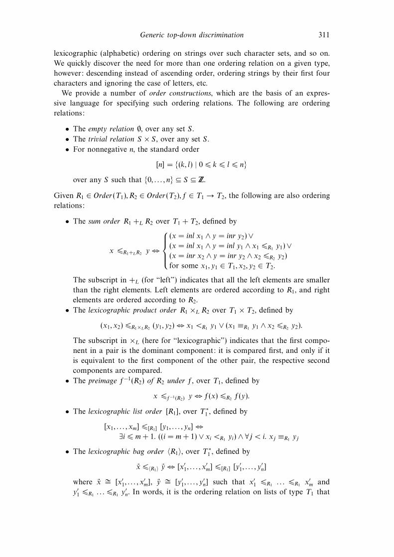
We provide a number of order constructions, which are the basis of an expres-

sive language for specifying such ordering relations. The following are ordering

relations:

• The empty relation 3, over any set S .

• The trivial relation S $ S , over any set S .

• For nonnegative n, the standard order

[n] = {(k, l) | 0 ! k ! l ! n}

over any S such that {0, . . . , n} # S # ".

Given R1 % Order(T1), R2 % Order(T2), f % T1 0 T2, the following are also ordering

relations:

• The sum order R1 +L R2 over T1 + T2, defined by

x !R1+LR2 y -

$%%&

%%'

(x = inl x1 ' y = inr y2) ,(x = inl x1 ' y = inl y1 ' x1 !R1 y1) ,(x = inr x2 ' y = inr y2 ' x2 !R2 y2)

for some x1, y1 % T1, x2, y2 % T2.

The subscript in +L (for “left”) indicates that all the left elements are smaller

than the right elements. Left elements are ordered according to R1, and right

elements are ordered according to R2.

• The lexicographic product order R1 $L R2 over T1 $ T2, defined by

(x1, x2) !R1$LR2 (y1, y2) - x1 <R1 y1 , (x1 .R1 y1 ' x2 !R2 y2).

The subscript in $L (here for “lexicographic”) indicates that the first compo-

nent in a pair is the dominant component: it is compared first, and only if it

is equivalent to the first component of the other pair, the respective second

components are compared.

• The preimage f&1(R2) of R2 under f, over T1, defined by

x !f&1(R2) y - f(x) !R2 f(y).

• The lexicographic list order [R1], over T (1 , defined by

[x1, . . . , xm] ![R1] [y1, . . . , yn] -2i ! m + 1. ((i = m + 1) , xi <R1 yi) ' 1j < i. xj .R1 yj

• The lexicographic bag order 4R15, over T (1 , defined by

!x !4R15 !y - [x*1, . . . , x

*m] ![R1] [y*

1, . . . , y*n]

where !x )= [x*1, . . . , x

*m], !y )= [y*

1, . . . , y*n] such that x*

1 !R1 . . . !R1 x*m and

y*1 !R1 . . . !R1 y

*n. In words, it is the ordering relation on lists of type T1 that

312 Fritz Henglein

arises from first sorting the lists in ascending order before comparing them

according to their lexicographic list order.

• The lexicographic set order {R1}, over T (1 , defined by

!x !{R1} !y - [x*1, . . . , x

*k] ![R1] [y*

1, . . . , y*l]

where x*1 <R1 . . . <R1 x*

k and y*1 <R1 . . . <R1 y*

l are maximal length proper

R1-chains of elements from !x and !y, respectively. In words, it is the ordering

relation on lists of type T1 that arises from first unique-sorting lists in ascending

order, which removes all .R1 -duplicates, before comparing them according to

their lexicographic list order.

• The inverse R&11 , over T1, defined by

x !R&11

y - x "R1 y.

Observe that the Cartesian product relation R1 $ R2 over T1 $ T2, with pointwise

ordering does not define an ordering relation. It satisfies transitivity (it is a preorder

on its definition set), but not conditional comparability.

Given dcpos D1, D2, recall that [D1 0 D2] denotes the dcpo of continuous

functions from D1 0 D2, ordered pointwise.

Theorem 1

Let T1, T2 be arbitrary sets. Then:

$L % [Order(T1) $ Order(T2) 0 Order(T1 $ T2)]

+L % [Order(T1) $ Order(T2) 0 Order(T1 + T2)

.&1 % (T1 0 T2) 0 [Order(T2) 0 Order(T1)]

[.] % [Order(T1) 0 Order(T (1 )]

4.5 % [Order(T1) 0 Order(T (1 )]

{.} % [Order(T1) 0 Order(T (1 )]

Proof

By inspection. We require / as the domain relation on ordering relations since $L

is nonmonotonic in its first argument under set containment #. !

Corollary 1

Let F % Order(T ) 0 Order(T ) be a function built by composing order constructions

in Theorem 1, the argument order and given ordering relations (“constants”). Then

F % [Order(T ) 0 Order(T )] and thus F has a least fixed point µF % Order(T ).

6 Order representations

In this section we show how to turn the order constructions of Section 5 into

a domain-specific language of order representations. These will eventually serve as

arguments to a generic order discriminator.


data Order t whereNatO :: Int -> Order IntTrivO :: Order tSumL :: Order t1 -> Order t2 -> Order (Either t1 t2)ProdL :: Order t1 -> Order t2 -> Order (t1, t2)MapO :: (t1 -> t2) -> Order t2 -> Order t1ListL :: Order t -> Order [t]BagO :: Order t -> Order [t]SetO :: Order t -> Order [t]Inv :: Order t -> Order t

Fig. 1. Order representations.

6.1 Basic order constructors

Definition 9 (Order representation)

An order representation over type T is a value r of type Order T constructible by

GADT in Figure 1, where all arguments f : T1 0 T2 to MapO occurring in a value

are total functions (that is f(x) "= 6 for all x % T1) and T1, T2 are first-order types.

Order representations are not ordering relations themselves, but tree-like data

structures denoting ordering relations. We allow infinite order representations. As we

shall see, such infinite trees allow representation of ordering relations on recursive

types.

An order expression is any Haskell expression, which evaluates to an order

representation. This gives us three levels of interpretation: A Haskell order expression

evaluates to an order representation, which is a data structure that denotes an

ordering relation. Note that not all Haskell expressions of type Order T are order

expressions, but henceforth we shall assume that all expressions of type Order Tthat we construct are order expressions.

6.2 Definable orders

Using the order constructors introduced, many useful orders and order constructors

are definable.

The standard order on the unit type () is its trivial order, which is also its only

order:

ordUnit :: Order ()ordUnit = TrivO

The standard ascending order on 8-bit and 16-bit non-negative numbers are

defined using the NatO-order constructor:4

4 Somewhat unconventionally, NatO n denotes the ascending standard ordering relation on {0 . . . n},not {0 . . . n & 1}. This reflects the Haskell convention of specifying intervals in the same fashion; e.g.newArray (0, 65535) [] allocates an array indexed by [0 . . . 65535]. Using the same conventionavoids the need for computing the predecessor in our Haskell code in a number of cases.

314 Fritz Henglein

ordNat8 :: Order IntordNat8 = NatO 255

ordNat16 :: Order IntordNat16 = NatO 65535

We might want to use

ordInt32W :: Order IntordInt32W = MapO tag (SumL (Inv (NatO 2147483648)) (NatO 2147483647))

where tag i = if i < 0 then Left (-i) else Right i

to denote the standard ordering on 32-bit 2s-complement integers.

(Note that 231 = 2147483648.) This does not work, since 2147483648 is not a 32-

bit 2s-complement representable integer, however. (Because NatO has type Int ->Order Int, where Int denotes the 32-bit 2s-complement representable integers, its

argument has to be a 32-bit integer.) Since the arguments of NatO are used by our ba-

sic discriminator as the size of a table to be allocated at run time, even if 2147483648

were acceptable, large argument values to NatO would be unusable in practice.

Instead we use the following order representation for the standard order on Int:

ordInt32 :: Order IntordInt32 = MapO (splitW . (+ (-2147483648))) (ProdL ordNat16

ordNat16)

splitW :: Int -> (Int, Int)splitW x = (shiftR x 16 .&. 65535, x .&. 65535)

Here we first add &231, the smallest representable 32-bit 2s complement integer, and

then split the resulting 32-bit word into its 16 high-order and low-order bits. The

lexicographic ordering on such pairs, interpreted as 16-bit non-negative integers,

then yields the standard ordering on 32-bit 2s-complement integers. As we shall

see, ordInt32 yields an e!cient discriminator that only requires a table with 216 =

65, 536 elements.

The standard order on Boolean values is denotable by the canonical function

mapping Bool to its isomorphic sum type:

ordBool :: Order BoolordBool = MapO bool2sum (SumL ordUnit ordUnit)

where bool2sum :: Bool -> Either () ()bool2sum False = Left ()bool2sum True = Right ()

Analogously, the standard alphabetic orders on 8-bit and 16-bit characters

are definable by mapping them to the corresponding orders on natural number

segments:

ordChar8 :: Order CharordChar8 = MapO ord ordNat8


ordChar16 :: Order CharordChar16 = MapO ord ordNat16

As an illustration of a denotable nonstandard order, here is a definition of

evenOdd, which denotes the ordering Oeo from Example 1:

evenOdd :: Order IntevenOdd = MapO (‘mod‘ 2) (NatO 1)

The SumL order lists left elements first. What about the dual order constructor,

where right elements come first? It is definable:

sumR :: Order t1 -> Order t2 -> Order (Either t1 t2)%sumR r1 r2 = Inv (SumL (Inv r1) (Inv r2)sumR r1 r2 = Inv (SumL (Inv r1) (Inv r2))

An alternative definition is

sumR’ r1 r2 = MapO flip (SumL r2 r1)where flip :: Either t1 t2 -> Either t2 t1

flip (Left x) = Right xflip (Right y) = Left y

Similarly, the lexicographic product order with dominant right component is defin-

able as

pairR :: Order t1 -> Order t2 -> Order (t1, t2)pairR r1 r2 = MapO swap (ProdL r2 r1)

where swap :: (t1, t2) -> (t2, t1)swap (x, y) = (y, x)

The refinement of equivalence classes of one order by another order is definable as

follows:

refine :: Order t -> Order t -> Order trefine r1 r2 = MapO dup (ProdL r1 r2)where dup x = (x, x)

For example, the nonstandard total order on 16-bit non-negative integers, where all

the even numbers, in ascending order, come first followed by all the odd numbers,

also in ascending order, is denoted by refine evenOdd ordNat16.

6.3 Lexicographic list order

For recursively defined data types, order representations generally need to be recur-

sively defined too. We first consider ListL, the lexicographic list order constructor,

and show that it is actually definable using the other order constructors. Then we

provide a general recipe for defining orders on regular recursive first-order types.

Consider the type T ( of T -lists with an element ordering R denoted by order

representation r. We want to define a representation of the lexicographic list order

[R]. We use Haskell’s standard list type constructor [T], with the caveat that only

T (, the finite lists, are intended even though Haskell lists may be infinite.

316 Fritz Henglein

We know that [t] is isomorphic to Either () (t, [t]), where

fromList :: [t] -> Either () (t, [t])fromList [] = Left ()fromList (x : xs) = Right (x, xs)

is the “unfold”-direction of the isomorphism. Assume we have a representation r*

of [R] and consider two lists !x,!y, where !x ![R] !y. Applying fromList to them, we

can see that the respective results are ordered according to SumL ordUnit (ProdLr r*). Conversely, if they are ordered like that, then !x ![R] !y. This shows that we

can define listL r by

listL :: Order t -> Order [t]listL r = r’

where r’ = MapO fromList (SumL ordUnit (ProdL r r’))

As an illustration of applying listL, the standard alphabetic order ordString8on String = [Char], restricted to 8-bit characters, is denotable by applying listLto the standard ordering on characters:

ordString8 :: Order StringordString8 = listL ordChar8

6.4 Orders on recursive data types

The general recipe for constructing an order representation over recursive types is

by taking the fixed point of an order constructor. Let p % [Order(T ) 0 Order(T )]

and take its least fixed point r = p(r). By Corollary 1 and standard domain-theoretic

techniques (Abramsky & Jung, 1992, Lemma 2.1.21), this r exists and denotes the

least fixed point of the function on ordering relations represented by p.

As an example, consider the type of node-labeled trees

data Tree v = Node (v, [Tree v])

with unfold-function

unNode :: Tree v -> (v, [Tree v])unNode (Node (v, ts)) = (v, ts)

The standard order on trees can be defined as

tree :: Order t -> Order (Tree t)tree r = r’

where r’ = MapO unNode (ProdL r (ListL r’))

It compares the root labels of two trees, and if they are r-equivalent, compares their

children lexicographically. This amounts to ordering trees by lexicographic ordering

on their preorder traversals.


As an example of a nonstandard order on trees, consider the level-k order treeKk on trees:

treeK :: Int -> Order t -> Order (Tree t)treeK 0 r = TrivOtreeK k r = Map unNode (ProdL r (ListL (treeK (k-1) r)))

It is the same as tree, but treats trees as equivalent if they are the same when “cut

o"” at level k.

Another example of an ordering relation on trees for a given node ordering is

treeB :: Order t -> Order (Tree t)treeB r = r’

where r’ = MapO unNode (ProdL r (BagO r’))

It treats the children of a node as an unordered bag in the sense that any permutation

of the children of a tree results in an equivalent tree. Finally,

treeS :: Order t -> Order (Tree t)treeS r = r’

where r’ = MapO unNode (ProdL r (SetO r’))

treats multiple equivalent children of a node as an unordered set: multiple children

that turn out to be equivalent are treated as if they were a single child.

Whether children of a node are treated as lists, bags, or sets in this sense is not

built into the data type, but can be freely mixed. For example

tree1 r = MapO unNode (ProdL r (ListL tree2 r))tree2 r = MapO unNode (ProdL r (BagO tree3 r))tree3 r = MapO unNode (ProdL r (SetO tree1 r))

interprets nodes at alternating levels as lists, bags, and sets, respectively.

6.5 Denotational semantics of order representations

So far we have informally argued that each order representation denotes an ordering

relation. In this section we provide the mathematical account of this. Basically, we do

this by interpreting each order constructor as the corresponding order construction.

Since order representations can be infinite trees, we need to be a bit careful.

We can leverage our domain-theoretic framework: We approximate each order

representation by cutting it o" at level k, show that the interpretations form an

#-chain, and define the interpretation of a order representation as the supremum

of its level-k approximations. Even though, domain-theoretically, the development

below is entirely standard, we give an explicit account as it forms the basis of the

definition of rank, which provides the basis for inductive proofs for structurally

recursively defined functions on order representations.5

5 This can be thought of as Scott induction, extended to make statements about termination.

318 Fritz Henglein

Definition 10 (Level-k approximation of order representation)

The level-k approximation r|k of order representation r is defined as follows:

r|0 = 6(NatO m)n+1 = NatO m

TrivOn+1 = TrivO

(SumL r1 r2)n+1 = SumL r1|n r2|n(ProdL r1 r2)n+1 = ProdL r1|n r2|n

(MapO f r)n+1 = MapO f r|n(ListL r)n+1 = ListL r|n(BagO r)n+1 = BagO r|n(SetO r)n+1 = SetO r|n(Inv r)n+1 = Inv r|n

for all m, n " 0, where 6 denotes the empty set.

Note that r|n is a finite tree of maximum depth n.

Recall the definition of order constructions from Section 5.

Definition 11 (Ordering relation denoted by order representation)

Let O[[r]] on finite order representations r be defined inductively as follows:

O[[6]] = 3O[[NatO m]] = [m]

O[[TrivO :: Order T]] =T $ T

O[[SumL r1 r2]] = O[[r1]] +L O[[r2]]

O[[ProdL r1 r2]] = O[[r1]] $L O[[r2]]

O[[MapO f r]] = f&1(O[[r]])

O[[ListL r]] = [O[[r]]]

O[[BagO r]] = 4O[[r]]5O[[SetO r]] = {O[[r]]}

O[[Inv r]] = O[[r]]&1

The ordering relation denoted by a possibly infinite order representation is

O[[r]] =(

n"0

O[[r|n]].

Theorem 2

Let r be an order representation over type T. Then O[[r]] is an ordering relation over

T .

Proof

We have O[[r|n]] / O[[r|n+1]] for all n " 0, and#

n"0 O[[r|n]] is the supremum. !


The level-k approximations provide a finitary stratification of pairs in the ordering

relation denoted by an order representation.

Definition 12 (Rank )

Let r % Order T. Let x, y % T , not necessarily distinct. The rank of x and y under r

is defined as

rank r(x, y) = min{n | (x, y) % O[[r|n]] , (y, x) % O[[r|n]]}

with rank r(x, y) = 7 if x#O[[r]] y. Define the rank of x under r by rank r(x) =

rank r(x, x).

Observe that rank r(x, y) = rank r(y, x); rank r(x, y) < 7 if and only if (x, y) %O[[r]] , (y, x) % O[[r]]; and rank r(x) < 7 if and only if x % def(O[[r]]). Note also that

the rank of a pair not only depends on the ordering relation but also on the specific

order representation to denote it.

Proposition 5

rank r(x, y) ! min{rank r(x), rank r(y)}

Proof

If (x, x) % O[[r|n]] , (y, y) % O[[r|n]] then (x, y) % O[[r|n]] , (y, x) % O[[r|n]] by

conditional comparability. Thus rank r(x, y) ! rank r(x) and rank r(x, y) ! rank r(y)

by Definition 12. !

The level-k approximations allow us to treat order representations as if they were

finite and prove results about them by structural induction. For example, consider

the functions comp, lte, csort and cusort as defined in Figure 2. We can prove that

comp implements the three-valued comparison function, lte the Boolean version of

comp, csort a sorting function, and cusort a unique-sorting function, in each case

for the order denoted by their respective first arguments. For comp, we specifically

have the following:

Proposition 6

For all order representations r :: Order T and x, y % T we have

comp r x y =

$%%&

%%'

LT if x <O[[r]] y

EQ if x .O[[r]] y

GT if x >O[[r]] y

6 if x#O[[r]] y

Proof

(Idea) We can prove by induction on n that the four functions have the desired

properties for all order representations r|n; e.g., comp r|n x y = EQ - x .O[[r|n]] y.

This works as each of the functions, when applied to r|n+1 on the left-hand side of

a clause, is applied to order representation(s) r*|n on the respective right-hand side.

From this the result follows for infinite r. !

320 Fritz Henglein

comp :: Order t -> t -> t -> Orderingcomp (NatO n) x y = if 0 <= x && x <= n && 0 <= y && y <= n

then compare x yelse error "Argument out of range"

comp TrivO _ _ = EQcomp (SumL r1 _) (Left x) (Left y) = comp r1 x ycomp (SumL _ _) (Left _) (Right _) = LTcomp (SumL _ _) (Right _) (Left _) = GTcomp (SumL _ r2) (Right x) (Right y) = comp r2 x ycomp (ProdL r1 r2) (x1, x2) (y1, y2) =

case comp r1 x1 y1 of { LT -> LT ;EQ -> comp r2 x2 y2 ;GT -> GT }

comp (MapO f r) x y = comp r (f x) (f y)comp (BagO r) xs ys = comp (MapO (csort r) (listL r)) xs yscomp (SetO r) xs ys = comp (MapO (cusort r) (listL r)) xs yscomp (Inv r) x y = comp r y x

lte :: Order t -> t -> t -> Boollte r x y = ordVal == LT || ordVal == EQ

where ordVal = comp r x y

csort :: Order t -> [t] -> [t]csort r = sortBy (comp r)

cusort :: Order t -> [t] -> [t]cusort r = map head . groupBy (lte (Inv r)) . sortBy (comp r)

Fig. 2. Generic comparison, sorting, and unique-sorting functions.

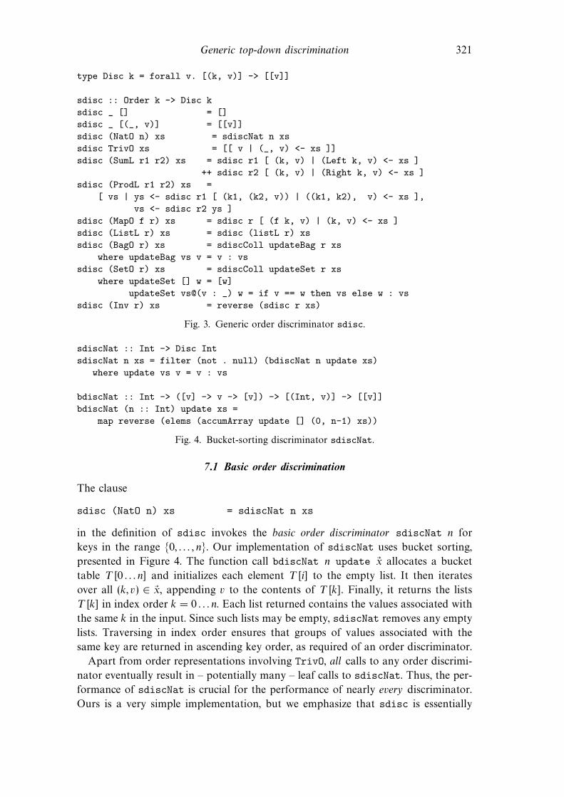
7 Generic order discrimination

Having defined and illustrated an expressive language for specifying orders, we are

now in a position to define the generic order discriminator sdisc. See Figure 3. We

discuss the clauses of sdisc below.

The type

type Disc k = forall v. [(k, v)] -> [[v]]

of a discriminator is polymorphic to capture its value parametricity property.

The clauses for the empty argument list, the trivial order, sum order, pre-image,

and inverse are self-explanatory. The innocuous-looking clause

sdisc _ [(_, v)] = [[v]]

is important for practical e!ciency: A call to sdisc with a singleton input pair

returns immediately without inspecting the key. This ensures that only distinguishing

parts of the keys need to be inspected during execution. In the specific case of

alphabetic string sorting, this implements the property of the most significant digit

first (MSD) lexicographic sorting of only inspecting the minimum distinguishing

prefix of keys in the input.


type Disc k = forall v. [(k, v)] -> [[v]]

sdisc :: Order k -> Disc ksdisc _ [] = []sdisc _ [(_, v)] = [[v]]sdisc (NatO n) xs = sdiscNat n xssdisc TrivO xs = [[ v | (_, v) <- xs ]]sdisc (SumL r1 r2) xs = sdisc r1 [ (k, v) | (Left k, v) <- xs ]

++ sdisc r2 [ (k, v) | (Right k, v) <- xs ]sdisc (ProdL r1 r2) xs =

[ vs | ys <- sdisc r1 [ (k1, (k2, v)) | ((k1, k2), v) <- xs ],vs <- sdisc r2 ys ]

sdisc (MapO f r) xs = sdisc r [ (f k, v) | (k, v) <- xs ]sdisc (ListL r) xs = sdisc (listL r) xssdisc (BagO r) xs = sdiscColl updateBag r xs

where updateBag vs v = v : vssdisc (SetO r) xs = sdiscColl updateSet r xs

where updateSet [] w = [w]updateSet vs@(v : _) w = if v == w then vs else w : vs

sdisc (Inv r) xs = reverse (sdisc r xs)

Fig. 3. Generic order discriminator sdisc.

sdiscNat :: Int -> Disc IntsdiscNat n xs = filter (not . null) (bdiscNat n update xs)

where update vs v = v : vs

bdiscNat :: Int -> ([v] -> v -> [v]) -> [(Int, v)] -> [[v]]bdiscNat (n :: Int) update xs =

map reverse (elems (accumArray update [] (0, n-1) xs))

Fig. 4. Bucket-sorting discriminator sdiscNat.

7.1 Basic order discrimination

The clause

sdisc (NatO n) xs = sdiscNat n xs

in the definition of sdisc invokes the basic order discriminator sdiscNat n for

keys in the range {0, . . . , n}. Our implementation of sdiscNat uses bucket sorting,

presented in Figure 4. The function call bdiscNat n update !x allocates a bucket

table T [0 . . . n] and initializes each element T [i] to the empty list. It then iterates

over all (k, v) % !x, appending v to the contents of T [k]. Finally, it returns the lists

T [k] in index order k = 0 . . . n. Each list returned contains the values associated with

the same k in the input. Since such lists may be empty, sdiscNat removes any empty

lists. Traversing in index order ensures that groups of values associated with the

same key are returned in ascending key order, as required of an order discriminator.

Apart from order representations involving TrivO, all calls to any order discrimi-

nator eventually result in – potentially many – leaf calls to sdiscNat. Thus, the per-

formance of sdiscNat is crucial for the performance of nearly every discriminator.

Ours is a very simple implementation, but we emphasize that sdisc is essentially

322 Fritz Henglein

parameterized in sdiscNat: Dropping in any high-performance implementation

essentially bootstraps its performance via sdisc to order discrimination for arbitrary

denotable ordering relations.

The code in Figure 4 implements the appending of a value to the contents of a

table bucket by actually prepending it and eventually reversing it. We remark that

eliding the final reversing of the elements of the array results in a reverse stable

order discriminator. It can be checked that reverse stable discriminators can also be

used in the remainder of the paper, saving the cost of list reversals. However, we

shall stick to stable discriminators for clarity and simplicity.

7.2 Lexicographic product order discrimination

Consider now the clause

sdisc (ProdL r1 r2) xs =[ vs | ys <- sdisc r1 [ (k1,(k2,v)) | ((k1,k2),v) <- xs ],

vs <- sdisc r2 ys ]

in Figure 3 for lexicographic product orders. First, each key-value pair is reshu%ed

to associate the second key component with the value originally associated with

the key. Then the reshu%ed pairs are discriminated on the first key component.

This results in a list of groups of pairs, each consisting of a second key component

and an associated value. Each such group is discriminated on the second key

component, and the concatenation of all the resulting value groups is returned. Note

how well the type of discriminators fits the compositional structure: We exploit the

ability of the discriminator on the first key component to work with any associated

values, and discarding the keys in the output of a discriminator makes the second

key component discriminator immediately applicable to the output of the first key

component discriminator.

7.3 Lexicographic list order discrimination

Lexicographic list order discrimination is implemented by order discrimination on

the recursively defined order constructor listL in Section 6.3:

sdisc (ListL r) xs = sdisc (listL r) xs

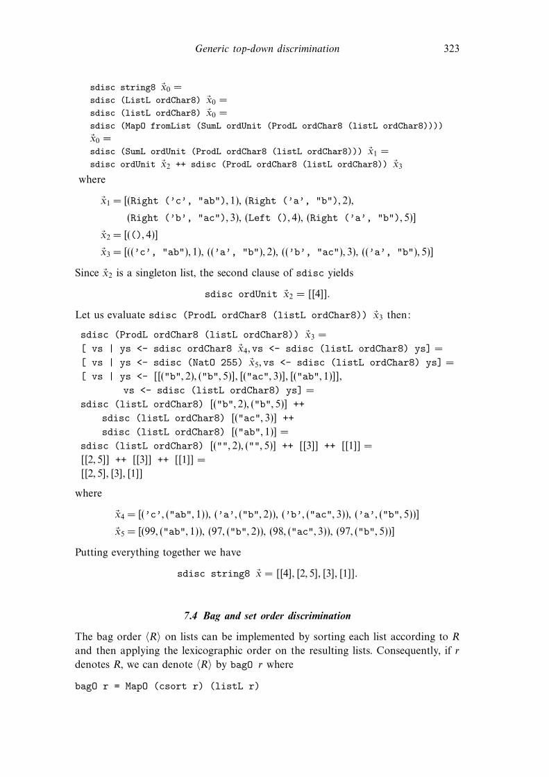
It is instructive to follow the execution of sdisc (listL r), since it illustrates

how an order representation functions as a control structure for invoking the

individual clauses of sdisc.

Example 2

Let us trace the execution of sdisc ordString8 on input

!x0 = [("cab", 1), ("ab", 2), ("bac", 3), ("", 4), ("ab", 5)].


sdisc string8 !x0 =sdisc (ListL ordChar8) !x0 =sdisc (listL ordChar8) !x0 =sdisc (MapO fromList (SumL ordUnit (ProdL ordChar8 (listL ordChar8))))

!x0 =sdisc (SumL ordUnit (ProdL ordChar8 (listL ordChar8))) !x1 =sdisc ordUnit !x2 ++ sdisc (ProdL ordChar8 (listL ordChar8)) !x3

where

!x1 = [(Right (’c’, "ab"), 1), (Right (’a’, "b"), 2),

(Right (’b’, "ac"), 3), (Left (), 4), (Right (’a’, "b"), 5)]

!x2 = [((), 4)]

!x3 = [((’c’, "ab"), 1), ((’a’, "b"), 2), ((’b’, "ac"), 3), ((’a’, "b"), 5)]

Since !x2 is a singleton list, the second clause of sdisc yields

sdisc ordUnit !x2 = [[4]].

Let us evaluate sdisc (ProdL ordChar8 (listL ordChar8)) !x3 then:

sdisc (ProdL ordChar8 (listL ordChar8)) !x3 =

[ vs | ys <- sdisc ordChar8 !x4, vs <- sdisc (listL ordChar8) ys] =

[ vs | ys <- sdisc (NatO 255) !x5, vs <- sdisc (listL ordChar8) ys] =

[ vs | ys <- [[("b", 2), ("b", 5)], [("ac", 3)], [("ab", 1)]],

vs <- sdisc (listL ordChar8) ys] =

sdisc (listL ordChar8) [("b", 2), ("b", 5)] ++sdisc (listL ordChar8) [("ac", 3)] ++sdisc (listL ordChar8) [("ab", 1)] =

sdisc (listL ordChar8) [("", 2), ("", 5)] ++ [[3]] ++ [[1]] =

[[2, 5]] ++ [[3]] ++ [[1]] =

[[2, 5], [3], [1]]

where

!x4 = [(’c’, ("ab", 1)), (’a’, ("b", 2)), (’b’, ("ac", 3)), (’a’, ("b", 5))]

!x5 = [(99, ("ab", 1)), (97, ("b", 2)), (98, ("ac", 3)), (97, ("b", 5))]

Putting everything together we have

sdisc string8 !x = [[4], [2, 5], [3], [1]].

7.4 Bag and set order discrimination

The bag order 4R5 on lists can be implemented by sorting each list according to R

and then applying the lexicographic order on the resulting lists. Consequently, if r

denotes R, we can denote 4R5 by bagO r where

bagO r = MapO (csort r) (listL r)

324 Fritz Henglein

and csort is the generic comparison-based sorting function from Figure 2. This

shows that, just like ListL, the order constructor BagO is redundant in the sense

that it is definable using the other order constructors, and we could define

sdisc (BagO r) xs = sdisc (bagO r) xs

as we have done for the lexicographic list order ListL. This typically6 yields an

O(N logN) algorithm, where N is the size of the input, for bag order discrimination.

We can do asymptotically better, however. The key insight is that, for the final

lexicographic list discrimination step in bag order processing, we only need the

ordinal number of an element of a key, not the element itself. This avoids reprocessing

of elements after sorting each of the keys.

Definition 13 (Ordinal number)

Let R be an ordering relation and K = [k1, . . . , kn], ki % def(R) for all i = 1, . . . , n.

The ordinal number NKR (ki) of ki under R within K is the maximum number of

pairwise R-inequivalent elements k* % K such that k* <R ki.

Example 3

1. Let K = [0, . . . , n] for n " 0. Let R = [n]. Then NKR (k) = k for all k % {0, . . . , n}.

2. Let K = [4, 9, 24, 11, 14] under the even-odd ordering Oeo in Example 1. Then

the ordinal number of 4, 24, and 14 is 0, and the ordinal number of 9 and 11

is 1.

Our discrimination algorithm for BagO r works as follows:

1. Given input [(!k1, v1), . . . , (!kn, vn)], with !ki = [ki1, . . . , kimi], sort the !ki according

to r, but return the ordinal numbers of their elements under r within

[k11, . . . , k1m1 , . . . kn1, . . . , knmn], instead of the elements themselves.

2. Perform lexicographic list order discrimination on listL (NatO l), where l is

the maximal ordinal number of any element in !k1 . . .!kn under r.

Step 1 is implemented e!ciently as follows:

1. Associate each key element kij with i, its key index.

2. Discriminate the (key element, key index) pairs under r. This results in groups

of key indices associated with .r-equivalent key elements, listed in ascending

r-order. Observe that the jth group in the result lists the indices of all the

keys that contain a key element with ordinal number j. Let l be the maximal

ordinal number of any key element.

3. Associate each key index with each of the ordinal numbers of its key elements.

4. Discriminate the (key index, ordinal number) pairs under NatO l. This results

in groups of ordinal numbers representing key elements of the same key, but

permuted into ascending order. We have to be careful to also return here

empty lists of ordinal numbers, not just nonempty lists.7 Since the groups are

6 See Section 14 for the use of “typically” here.7 This was pointed out by an anonymous referee.


sdiscColl :: ([Int] -> Int -> [Int]) -> Order k -> Disc [k]sdiscColl update r xss = sdisc (listL (NatO (length keyNumBlocks - 1))) yss

where(kss, vs) = unzip xsselemKeyNumAssocs = groupNum ksskeyNumBlocks = sdisc r elemKeyNumAssocskeyNumElemNumAssocs = groupNum keyNumBlockssigs = bdiscNat (length kss) update keyNumElemNumAssocsyss = zip sigs vs

Fig. 5. Bag and set order discrimination.

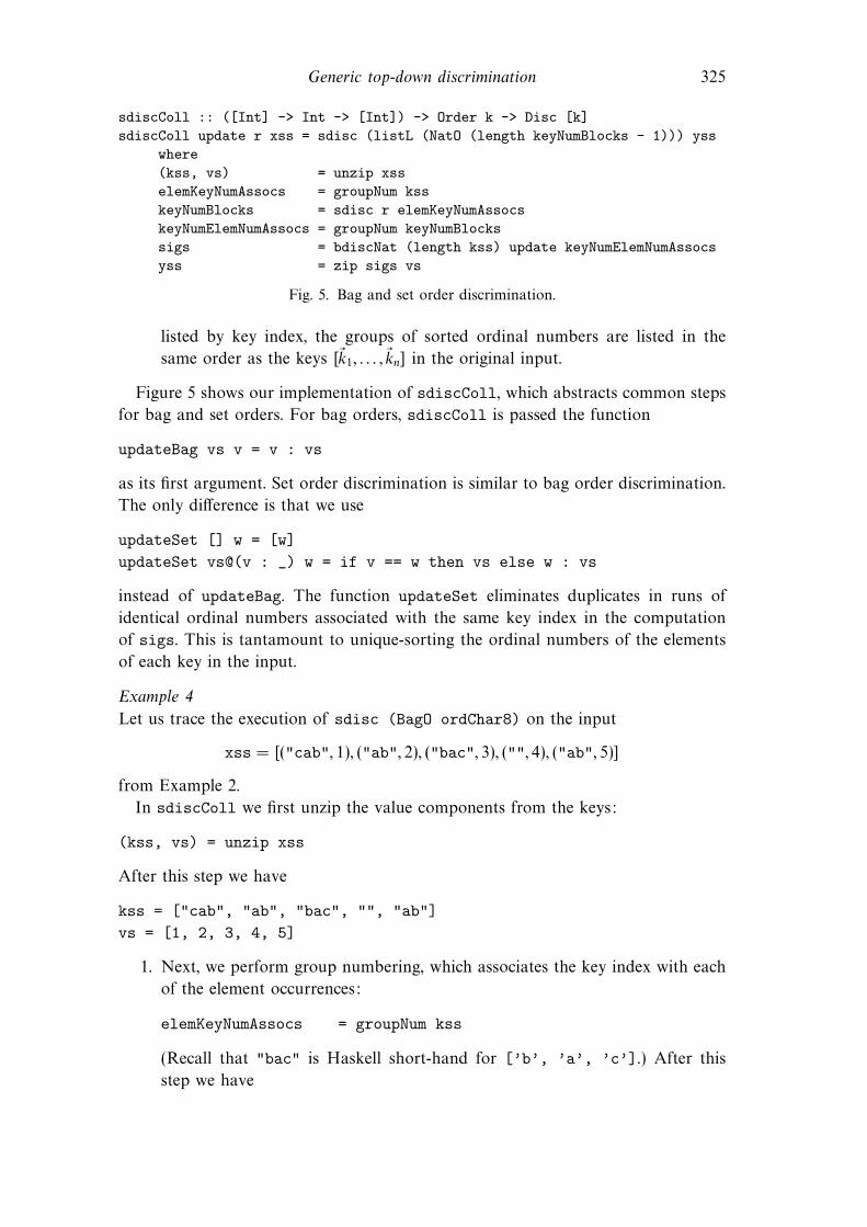
listed by key index, the groups of sorted ordinal numbers are listed in the

same order as the keys [!k1, . . . ,!kn] in the original input.

Figure 5 shows our implementation of sdiscColl, which abstracts common steps

for bag and set orders. For bag orders, sdiscColl is passed the function

updateBag vs v = v : vs

as its first argument. Set order discrimination is similar to bag order discrimination.

The only di"erence is that we use

updateSet [] w = [w]updateSet vs@(v : _) w = if v == w then vs else w : vs

instead of updateBag. The function updateSet eliminates duplicates in runs of

identical ordinal numbers associated with the same key index in the computation

of sigs. This is tantamount to unique-sorting the ordinal numbers of the elements

of each key in the input.

Example 4

Let us trace the execution of sdisc (BagO ordChar8) on the input

xss = [("cab", 1), ("ab", 2), ("bac", 3), ("", 4), ("ab", 5)]

from Example 2.

In sdiscColl we first unzip the value components from the keys:

(kss, vs) = unzip xss

After this step we have

kss = ["cab", "ab", "bac", "", "ab"]vs = [1, 2, 3, 4, 5]

1. Next, we perform group numbering, which associates the key index with each

of the element occurrences:

elemKeyNumAssocs = groupNum kss

(Recall that "bac" is Haskell short-hand for [’b’, ’a’, ’c’].) After this

step we have

326 Fritz Henglein

elemKeyNumAssocs = [(’c’, 0), (’a’, 0), (’b’, 0),(’a’, 1), (’b’, 1),(’b’, 2), (’a’, 2), (’c’, 2),(’a’, 4), (’b’, 4) ].

2. We discriminate these pairs according to the key element ordering ordChar8:

keyNumBlocks = sdisc ordChar8 elemKeyNumAssocs

which results in

keyNumBlocks = [ [0, 1, 2, 4], [0, 1, 2, 4], [0, 2] ]

in our example. The first group corresponds to key character ’a’, the second

to ’b’, and the third to ’c’. The elements of each group are the indices,

numbered 0, . . . , 4, of keys, in which a member of the particular equivalence

class occurs; for example, 0 is the index of "cab" and 2 of "bac". So the group

[0, 2] in keyNumBlocks expresses that the equivalence class represented by

that group (the character ’c’) occurs once in the key with index 0 ("cab")and once in the key with index 2 ("bac"), and in no other keys. Note that 3

does not occur in keyNumBlocks at all, since the key with index 3 is empty.

3. Next we convert keyNumBlocks into its group number representation:

keyNumElemNumAssocs = groupNum keyNumBlocks,

which results in the binding

keyNumElemAssocs = [ (0, 0), (1, 0), (2, 0), (4, 0),(0, 1), (1, 1), (2, 1), (4, 1),(0, 2), (2, 2) ].

Each pair (i, j) represents an element containment relation: the key with index

i contains an element with ordinal number j. For instance, the pair (4, 0)expresses that the key with index 4, the second occurrence of "ab", contains

an element with ordinal number 0, the character ’a’.4. We now discriminate these membership pairs:

sigs = bdiscNat 5 updateBag keyNumElemNumAssocs

This collects together all the characters, represented by their ordinal numbers,

that are associated with the same key. Each group thus represents a key

from the input, but with each character replaced by its ordinal number. Using

bdiscNat ensures that the groups are returned in the same order as the keys

in kss and that empty value lists are returned too. Since bdisc is stable, it

returns the ordinal numbers in ascending order in each group. The resulting

groups of ordinal numbers in our example are

sigs = [ [0, 1, 2], [0, 1], [0, 1, 2], [], [0, 1] ].

Observe that they represent the original keys kss, but each key ordered

alphabetically into


["abc", "ab", "abc", "", "ab"]

and with ordinal numbers replacing the corresponding key elements.

Finally, we zip sigs with the value components vs from the original xss:

yss = zip sigs vs.

This gives

yss = [([0,1,2], 1), ([0,1], 2), ([0,1,2], 3), ([], 4), ([0,1], 5)]

Applying the list order discriminator

sdisc (listL (NatO (length keyNumBlocks - 1))) yss

where length keyNumBlocks - 1= 2, the final output is [ [4], [2, 5], [1, 3] ].

Observe how bag and set order discrimination involves a discrimination step on

key elements, which may result in recursive discrimination of nodes inside those

elements, and two other discrimination steps on key indices and lists of ordinal

numbers, respectively, which do not recurse into the keys.

7.5 Correctness

Theorem 3

For each order representation r :: Order T, sdisc r is a stable order discriminator

for O[[r]] over T .

Proof

(Sketch) By induction on n = max{rank r(ki) | i % {1, . . . , n}} where [(k1, v1), . . . , (kn, vn)]

is the input to sdisc r. The case for rank 0 is vacuously true. For the inductive case,

we inspect each clause of sdisc in turn. In each case, the maximum rank of keys in

a call to sdisc on the right-hand side is properly less than the maximum rank of

the keys in the call on the left-hand side, which allows us to invoke the induction

hypothesis, and we can verify that the values in the result are grouped as required

of a stable order discriminator for O[[r]]. !

8 Complexity

In this section we prove that sdisc from Figure 3 typically produces worst-

case linear-time order discriminators. In particular, it does so for the standard

ordering relations on all regular recursive first-order types and thus yields linear-

time partitioning and sorting algorithms for each.

Our machine model is a unit-cost random access machine (RAM) (Tarjan, 1983)

with fixed word width, where values are stored in fully boxed representation. It has

basic instructions operating on constant-size data. In particular, operations on pairs

(construction, projection), tagged values (tagging, pattern matching on primitive

tags), and iso-recursive types (folding, unfolding) each take constant time. Unit-cost

means that pointer operations and operations on “small” integers – integer values

328 Fritz Henglein

polynomially bounded by the size of the input – take constant time. Random access

means that array lookups using small integers as indices also take constant time.

Fixed word width means that the number of bits per word in RAM memory is

constant (think 32 or 64). In particular, it does not change depending on the size of

the input.

We define the size of a value as follows.

Definition 14 (Size)

The (tree) size of a value is defined as follows:

|c| = 1

|()| = 1

|inl v| = 1 + |v||inr w| = 1 + |w||(v, w)| = 1 + |v| + |w|

|fold (v)| = 1 + |v|

Note that the size function for pairs adds the size of each component separately.

This means that the size function measures the storage requirements of an unshared

(unboxed or tree-structured ) representation asymptotically correctly, but not of

shared data: A directed acyclic graph (dag) with n elements may represent a tree of

size #(2n). The size function will consequently yield #(2n) even though the dag can

be stored in space O(n). The top–down (purely recursive) method embodied in our

generic discriminators in this paper gives asymptotically optimal performance only

for unshared data. Dealing with sharing e!ciently requires bottom–up discrimination

(Paige, 1991; Henglein, 2003), which builds upon top–down discrimination. Generic

bottom–up discrimination is future work.

We write Tf(v) for the number of steps function f takes on input v.8

Definition 15

The set L of linear-time discriminable order representations is the set of all order

representations r such that

Tsdisc r ([(k1, v1), . . . , (kn, vn)]) = O(n +)n

i=1 |ki|).

8.1 Nonrecursive orders

The question now is as follows: Which order representations are linear-time dis-

criminable? Clearly, a function f must execute in linear time if the discriminator for

MapO f r is to do so, too. Interestingly this is su!cient to guarantee that each

finite order representation yields a linear-time discriminator.

8 Here, we use “function” in the sense of code implementing a mathematical function.


Proposition 7

Let r be a finite order representation, where each function occurring in r executes in

linear time and produces an output of size linear in its input. Then r is linear-time

discriminable.

Proof

By structural induction on r. The key property is that a linear-time executable

function f used as an argument to MapO in r can only increase the size of its output

by a constant factor relative to the size of its input. Note that the output size

limitation does not follow from f executing in linear time, since it may produce a

shared data structure with exponentially larger tree size. !

It is important to note that the constant factor in the running time of sdiscr generally depends on r. So this result does not immediately generalize to order

representations for recursive types.

8.2 Recursive orders

To get a sense of when an infinite order representation yields a linear-time order

discriminator, let us investigate a situation where this does not hold.

Consider the order constructor flipflop

flipflop :: Order t -> Order [t]flipflop r = MapO (fromList . reverse)

(SumL ordUnit (ProdL r (flipflop r)))

It orders lists lexicographically, but not by the standard index order on elements

in the list. It first considers the last element of the list, then the first, then next-to-

last, second, next-to-next-to-last, third, etc. Applying sdisc to flipflop ordChar8yields a quadratic time discriminator. The reason for this is the repeated appli-

cation of the reverse function. We can observe that the comparison function

comp (flipflop ordChar8) also takes quadratic time.

Let us look at the body of flipflop in more detail: We have an order

representation r that satisfies

r* = MapO (fromList . reverse) (SumL ordUnit (ProdL r r* )).

Executing sdisc r* causes sdisc r* to be executed recursively. The reason for

nonlinearity is that the recursive call operates on parts of the input that are also

processed by the nonrecursive code, specifically by the reverse function.

The key idea to ensuring linear-time performance of recursive discriminators is

the following: Make sure that the input can be (conceptually) split such that the

execution of the body of sdisc r* minus its recursive calls to the same discriminator

sdisc r* can be charged to one part of the input, and its recursive call(s) to the

other part. Charging means that we attribute a constant amount of computation to

constant amounts of the original input. In other words, the nonrecursive computation

steps are not allowed to “touch” those parts of the input that are passed to the

recursive call(s): They may maintain and rearrange the pointers to those parts, but

330 Fritz Henglein

must not de-reference them. How can we ensure that this is obeyed? We insist that

the nonrecursive computation steps of sdisc r* only manipulate pointers to the parts

passed to the recursive calls of sdisc r* without de-referencing or duplicating them.

Intuitively, the nonrecursive code must be parametric polymorphic in the original

sense of Strachey (2000)!

The main technical complication is extending this idea to order representations

containing MapO. We do this by conceptually splitting the input keys, viewed from

their roots, into top-level parts, which are processed nonrecursively, and bottom-level

parts, which are passed to the recursive call(s).

To formalize this splitting idea, we extend types and order representations with

formal type variables t1, t2, ..., tn and order variables r1, r2, ..., rnrespectively. For simplicity, we restrict ourselves to adding a single type variable t1and a single order variable r1 of type Order t1 here.

Definition 16

Let t1 be a distinct type variable and r1 a formal order variable.

Then the types T7[t1] over t1 are the set of possibly infinite labeled trees built

from the signature

{A(0),$(2),+(2), 1(0), foldT (1), t10}.R7[r1] is the set of typed labeled trees built from the constructors in Defini-

tion 9 with an additional formal constructor r1 :: Order t1. Furthermore, each

f occurring in R % R7[r1] must have polymorphic type 1t1.T1 0 T2 for some

T1, T2 % T7[t1].

We can now split the size of a value of type T % T7[t1] into upper and lower

parts.

Definition 17 (Upper and lower sizes)

Let T % T7[t1]. The lower and upper sizes |.|T , respectively |.|T , are defined as

follows:

|v|t1 = 0

|c|A = 1

|()|1 = 1

|inl v|T1+T2 = 1 + |v|T1

|inr w|T1+T2 = 1 + |w|T2

|(v, w)|T1$T2 = 1 + |v|T1 + |w|T2

|fold (v)|µt.T = 1 + |v|T [(µt.T )/t]

|v|t1 = |v||c|A = 0

|()|1 = 0

|inl v|T1+T2 = |v|T1


|inr w|T1+T2 = |w|T2

|(v, w)|T1$T2 = |v|T1 + |w|T2

|fold (v)|µt.T = |v|T [(µt.T )/t]

Proposition 8

For all values v and types T % T7[t1] we have |v| = |v|T + |v|T whenever both

sides are defined.

Proof

By complete (course of values) induction on |v|. !

The key property for proving linear-time discriminability for infinite order rep-

resentations is that polymorphic functions occurring in MapO order representations

must be linear-time computable in a strong sense.

Definition 18 (Strongly linear-time computable function)

We say a function f :: 1t1.T1 0 T2 is strongly linear-time computable if

1. Tf(k) = O(|k|T1 ).

2. |f(k)|T2 = O(|k|T1 ).

3. |f(k)|T2 ! |k|T1 .

Note that the last condition is without O.

Here are some examples of linear-time computable functions:

• The identity function id :: 1t1.t1 0 t1.• The list length function length :: 1t1.[t1] 0 Int.

• The list reverse function reverse :: 1t1.[t1] 0 [t1].

The argument duplication function dup :: 1t1.t1 0 t1 $ t1, on the other hand,

is not linear-time computable: it violates the third condition in Definition 18.

Since we measure the tree size of values, a function can produce outputs of

asymptotically larger size than its running time because of sharing. Consider the

function repFstElem :: 1t.[t] 0 [t], which takes as input [v1, . . . , vn] and returns

[

n* +, -v1, . . . , v1] for n " 1. Applying it to a list with a first element of size m, followed

by m elements of size 1 yields a result of size #(m2). It satisfies Property 1 but

not Property 2 (nor Property 3 for that matter). This shows that Property 1 of

Definition 18 does not imply Property 2.

We can now give a recipe for constructing order representations over recursive

types that yield linear-time discriminators:

1. Let T = µt1.T * be a recursive type with f : T 0 T *[T/t1], f(fold (v)) = v the

unfold part of the isomorphism between T and T *[T/t1].2. Find a finite order representation r* :: Order T * containing only strongly

linear-time computable functions.

3. Define r :: Order T recursively by r = MapO f r*[r/r1].

Then R is linear-time discriminable. We sketch a proof of this below.

332 Fritz Henglein

Definition 19 (T1)

Define T1sdisc r*[r/r1]

(!x) to be the execution time of sdisc r*[r/r1](!x), but not

counting any calls of the form sdisc r (!y).

Lemma 1

Let T = µt1.T *. Let r :: Order T , r* :: Order T * finite, and let all functions f

occurring in r* be strongly linear-time computable. Then

1. T1sdisc r*[r/r1]

(!x) = O(n +)n

i=1 |ki|T*) where !x = [(k1, v1), . . . , (kn, vn)].

2. The bag of calls 4sdisc r (!zj)5j invoked during execution of sdisc r*[r/r1](!x)

has the property that)

j |!zj | !)n

i=1 |ki|T * .

Proof

(Sketch) The proof is by structural induction on r*. The most interesting cases are

MapO f r**, ListL r**, BagO r**, and SetO r**.

• For MapO f r** the requirement of strong linear-time computability of f is

su!cient to make the induction step go through.

• For ListL r**, consider the recursive applications of sdisc during evaluation

of sdisc (ListL r**)!x. Let us charge the nonrecursive computation steps

of a call to sdisc r*** (for any r***) to the roots (only!) of the keys in the

input. (Recall that we assume a fully boxed data representation. The space

requirement of each node of such a representation is accounted for by the

additive constant 1 in Definition 14.) It is straightforward to check that each

node is then charged with a constant number of computation steps, since each

node occurs at the most once as the root of a key in the input of a call to

sdiscr*** for some r*** during the evaluation of sdisc (ListL r**)!x.

• For BagO r**, the first part of the lemma follows from the fact that, by

definition, sdisc (BagO r) consists of one invocation of sdisc r, which,

inductively, executes in linear time in the aggregate size of the key elements

of the input; and the remaining steps, which are linear in the size of the

remaining nodes in the input. For the second part of the lemma, it is important

that only the call to sdisc r operates on key elements, and the final call

sdisc (ListL . . . ) yss is on the ordinal numbers of the key elements, not

the key elements themselves.

• For SetO r** the argument is the same as for BagO r**. #

We can now apply Lemma 1 recursively.

Theorem 4

Let T = µt1. T * with f :: T 0 T *[T/t1], f(fold (v)) = v, the unfold-function from

T . Let r :: Order T and finite r* :: Order T * such that

r = MapO f (r*[r/r1]).

Furthermore, let all functions occurring in r* be strongly linear-time computable.

Then r is linear-time discriminable.


ProofConsider sdisc r (!x) where !y = [(f(k), v)|(k, v) %!x].

Tsdisc r(!x) = Tsdisc MapO f (r*[r/r1])(!x)

= Tsdisc r*[r/r1](!y) + O(n.

i=1

|ki|T*) by properties of f

= T1sdisc r*[r/r1](!y) + O(

n.

i=1

|ki|T*) + all recursive calls to sdisc r

=O(n.

i=1

|ki|T*) + O(

n.

i=1

|ki|T*) +

.

j

Tsdisc r(!zj)

=O(n.

i=1

|ki|T*) +

.

j

Tsdisc r(!zj)

where)

j |!zj | !)n

i=1 |ki|T * by Lemma 1. Since |!x| ")n

i=1 |ki| =)n

i=1 |ki|T*+)n

i=1 |ki|T * , we can see that the number of the execution steps excepting the recursive

ones to sdisc r is linear bounded by one part of the input, and all the recursive calls

of sdisc r can be attributed to the other part of the input, with the same constant

factor. Consequently, the whole execution is linear bounded in the size of the keys

in the input, and thus sdisc r is linear-time discriminable. !

Each regular recursive type T has a standard order rT denoted by a canonical

order representation: product types are ordered by ProdL, sum types by SumL,Int by its standard order, t1 by r1, and a recursive type T = µt1. T * by r =

MapO f (r*[r/r1]), where r* is the canonical order representation for T * and f is the

unfold-function from T to T *[T/t1].

Corollary 2Let T be a regular recursive first-order type. Then rT , the canonical order represen-

tation for T , is linear-time discriminable.

ProofThe conditions of Theorem 4 are satisfied. !

We have observed that whenever a discriminator is superlinear, so is the compar-

ison function. We conjecture that sdisc has the same asymptotic behavior as the

generic binary comparison function comp (see Figure 2).

Conjecture 1Let T*

comp r(n) = max{Tcomp r(x1)(x2) | |x1| + |x2| ! n} and

T*sdisc r(n) = max{Tsdisc r([(k1, v1), . . . , (km, vm)]) |

)mi=1 |ki| ! n}.

Then T*sdisc r = O(Tcomp r).

The conjecture expresses that discriminators are a proper generalization of the

corresponding comparison functions for all R, not just the linear-time discriminable:

They asymptotically execute within the same computational resource bounds, but

decide the ordering relation on m arguments (of aggregate size n) instead of just two

arguments (of combined size n).

334 Fritz Henglein

9 Equivalence representations

In the previous sections we have seen how to implement order discrimination

e!ciently by structural recursion over order representations. In this section we shall

do the same for equivalences. The presentation is condensed where the techniques

are essentially the same as for order discrimination. We emphasize that the practical

benefits of equivalence discrimination are most pronounced for references, which

have no natural ordering relation, and for problems where the output is not required

to be ordered.

9.1 Equivalence constructors

As for ordering relations (Section 6), there are common constructions on equivalence

relations. The following are equivalence relations:

• The empty relation 3, on any set S .• The trivial relation S $ S , on S .• For each nonnegative n, the identity relation .[n] on {0, . . . n}.

Given E1 % Equiv (T1), E2 % Equiv (T2), andf % T1 0 T2, the following are also

equivalence relations:

• The sum equivalence E1 +E E2, over T1 + T2, defined by

x .E1+EE2 y -

$&

'

(x = inl x1 ' y = inl y1 ' x1 .E1 y1) ,(x = inr x2 ' y = inr y2 ' x2 .E2 y2)

for some x1, y1 % T1, x2, y2 % T2.

• The product equivalence E1 $E E2, over T1 $ T2, defined by

(x1, x2) .E1$EE2 (y1, y2) - x1 .E1 y1 ' x2 .E2 y2.

• The pre-image f&1(E2) of E2 under f, over T1, defined by

x .f&1(E2) y - f(x) .E2 f(y).

• The list equivalence .[E1], also written E(1 , over T (

1 , defined by

[x1, . . . , xm] .[E1] [y1, . . . , yn] -m = n ' 11 ! j ! m. xj .E1 yj

• The bag equivalence .4E15 on T (1 , over T (

1 , defined by

!x .4E15 !y - 2x*.!x )=!x* '!x* .[E1] !y.

(Recall that !x )=!x* means that !x* is permutation of !x.)• The set equivalence {E1} on T (

1 , over T (1 , defined by

!x .{E1} !y - (1i.2j. xi .E1 yj) ' (1j.2i. xi .E1 yj).

Treating the equivalence constructions as constructors, we can define equivalence

representations the same way as we have done for order representations. See Figure 6.

Using domain-theoretic arguments as for order representations (Theorems 1 and 2),


data Equiv t whereNatE :: Int -> Equiv IntTrivE :: Equiv tSumE :: Equiv t1 -> Equiv t2 -> Equiv (Either t1 t2)ProdE :: Equiv t1 -> Equiv t2 -> Equiv (t1, t2)MapE :: (t1 -> t2) -> Equiv t2 -> Equiv t1ListE :: Equiv t -> Equiv [t]BagE :: Equiv t -> Equiv [t]SetE :: Equiv t -> Equiv [t]

Fig. 6. Equivalence representations.

eq :: Equiv t -> t -> t -> Booleq (NatE n) x y = if 0 <= x && x <= n && 0 <= y && y <= n

then (x == y)else error "Argument out of range"

eq TrivE _ _ = Trueeq (SumE e1 _) (Left x) (Left y) = eq e1 x yeq (SumE _ _) (Left _) (Right _) = Falseeq (SumE _ _) (Right _) (Left _) = Falseeq (SumE _ e2) (Right x) (Right y) = eq e2 x yeq (ProdE e1 e2) (x1, x2) (y1, y2) =

eq e1 x1 y1 && eq e2 x2 y2eq (MapE f e) x y = eq e (f x) (f y)eq (ListE e) xs ys = eq (listE e) xs yseq (BagE _) [] [] = Trueeq (BagE _) [] (_ : _) = Falseeq (BagE e) (x : xs’) ys =

case delete e x ys of Just ys’ -> eq (BagE e) xs’ ys’Nothing -> False

wheredelete :: Equiv t -> t -> [t] -> Maybe [t]delete e v = subtract’ []

where subtract’ _ [] = Nothingsubtract’ accum (x : xs) =

if eq e x v then Just (accum ++ xs)else subtract’ (x : accum) xs

eq (SetE e) xs ys =all (member e xs) ys && all (member e ys) xswhere member :: Equiv t -> [t] -> t -> Bool

member _ [] _ = Falsemember e (x : xs) v = eq e v x || member e xs v

Fig. 7. Generic equivalence test.

each equivalence representation e, whether finite or infinite, denotes an equivalence

relation E[[e]].

Theorem 5

Let e be an equivalence representation. Then E[[e]] is an equivalence relation.

Analogous to Proposition 6, it is possible to characterize E[[e]] by the generic

equivalence testing function eq :: Equiv t -> t -> t -> Bool in Figure 7.

336 Fritz Henglein

Proposition 9

For all equivalence representations e over T , x, y % T

eq e x y =

$&

'

True if x .O[[e]] y

False if x ".O[[e]] y ' (x % def(e) , y % def(e))

6 if x ".O[[e]] y ' x "% def(e) ' x "% def(e)

9.2 Definable equivalence constructors

We can denote the identity relations (equality) on basic types:

eqUnit :: Equiv ()eqUnit = TrivE

eqBool :: Equiv BooleqBool = MapE bool2sum (SumE eqUnit eqUnit)

where bool2sum :: Bool -> Either () ()bool2sum False = Left ()bool2sum True = Right ()

eqNat8 :: Equiv InteqNat8 = NatE 255

eqNat16 :: Equiv InteqNat16 = NatE 65535

eqInt32 :: Equiv InteqInt32 = MapE splitW (ProdE eqNat16 eqNat16)

eqChar8 :: Equiv ChareqChar8 = MapE ord eqNat8

eqChar16 :: Equiv ChareqChar16 = MapE ord eqNat16

Observe how equality representation eqInt32 on 32-bit integers is defined in what

appears to be a rather roundabout fashion: It splits integers into their upper and

lower 16 bits and then performs equality on these pairs componentwise as unsigned

16-bit integers. (Function splitW is defined in Section 6.2.) The reason for this is as

given above: to enable e!cient basic discrimination by using a bucket array indexed

by 16-bit integers. This can also be done using 8, 24, or any other number of bits,

or any combination thereof, but we shall restrict ourselves to 16-bit indexed arrays

for simplicity.

The general recipe for defining equivalence representations on recursive types is

the same as for order representations in Section 6.4. In particular, list equivalence is

definable as follows:


disc :: Equiv k -> Disc kdisc _ [] = []disc _ [(_, v)] = [[v]]disc (NatE n) xs =

if n < 65536 then discNat16 xs else disc eqInt32 xsdisc TrivE xs = [map snd xs]disc (SumE e1 e2) xs = disc e1 [ (k, v) | (Left k, v) <- xs ] ++

disc e2 [ (k, v) | (Right k, v) <- xs ]disc (ProdE e1 e2) xs =

[ vs | ys <-disc e1 [ (k1, (k2, v)) | ((k1, k2), v) <- xs ],vs <- disc e2 ys ]

disc (MapE f e) xs = disc e [ (f k, v) | (k, v) <- xs ]disc (ListE e) xs = disc (listE e) xsdisc (BagE e) xs = discColl updateBag e xsdisc (SetE e) xs = discColl updateSet e xs

Fig. 8. Generic equivalence discriminator disc.

listE :: Equiv t -> Equiv [t]listE e = MapE fromList (SumE eqUnit (ProdE e (listE e)))

where fromList is as in Section 6.3. Using listE we can define string equality:

eqString8 :: Equiv StringeqString8 = list eqChar8

10 Generic equivalence discrimination

We can now give the complete definition of the generic equivalence discriminator

disc, which is indexed by equivalence representations; see Figure 8. Let us look at

the main di"erences to sdisc.

10.1 Basic equivalence discrimination

A basic equivalence discriminator is like the bucket-sorting-based order discriminator

sdiscNat n from Figure 4, with the exception that it returns the groups in the order

the keys occur in the input, instead of ordered numerically. It can be implemented

as follows. When applied to key-value pairs !x:

1. Allocate a bucket table T [0 . . . n] and initialize each bucket to the empty list.

Allocate variable K for holding a key list, also initialized to the empty list.

2. Iterate over all (k, v) %!x, appending v to T [k], and if k is encountered for the

first time, append k to K .

3. Iterate over all keys k % K , outputting T [k].

Figure 9 shows an implementation in Haskell using the ST monad, which allows

encapsulating the imperative updates to a locally allocated array as an observably

side e"ect free function. Even though the final index order traversal is avoided, it

still su"ers from the same deficit as sdiscNat: Every application discNatST n !x

results in the allocation and complete initialization of a bucket table T [0 . . . n].

338 Fritz Henglein

discNatST :: Int -> Disc IntdiscNatST n xs =runST (

do table <- newArray (0, n) [] :: ST s (STArray s Int [v]) ;ks <- foldM (\keys (k, v) ->

do vs <- readArray table k ;case vs of [] -> do writeArray table k [v] ;

return (k : keys) ;_ -> do writeArray table k (v : vs) ;

return keys )[] xs ;

foldM (\vss k -> do elems <- readArray table k ;return (reverse elems : vss) )

[] ks)

Fig. 9. Basic equivalence discriminator implemented using ST monad Not used – tooine!cient!.

Paige & Tarjan (1987) employ the array initialization trick of Aho et al. (1983)

to get around complete table initialization. We can go one step further: Avoid

allocation of a new bucket table for each call altogether. The key idea is to use

a global bucket table T [0 . . . n], whose elements are guaranteed to be empty lists

before and after a call to the basic equivalence discriminator.

We define a function discNat, which generates e!cient basic equivalence discrim-

inators. A call to discNat n does the following:

1. Allocate a bucket table T [0 . . . n] and initialize each element to the empty list.

2. Return a function that, when passed key-value pairs !x, executes the following:

(a) Allocate a variable K for a list of keys, initialized to the empty list.

(b) Iterate over all (k, v) %!x, appending v to T [k], and if k is encountered

for the first time, appending k to K .

(c) Iterate over all keys k % K , outputting T [k], and resetting T [k] to the

empty list.

Note that executing discNat n allocates a bucket table and returns a function,

where each call reuses the same bucket table. The function requires that the bucket

table contains only empty lists before executing the above-mentioned first step (2a);

it re-establishes this invariant in the final step (2c). The upshot is that the function

does not allocate a new table every time it is called and executes in time O(|!x|),independent of n, instead of O(|!x| + n), which is critical for practical performance.

The basic discriminator returned by a call to discNat n is neither re-entrant nor

thread-safe nor resilient to exceptions thrown during its execution because of the

possibility of unsynchronized accesses and imperative updates to the bucket table

shared by all calls. Consequently, each thread should use a basic discriminator with a

thread-local bucket table, and, in a language with lazy evaluation such as Haskell, all

keys in the input should be fully evaluated before the first key is stored in the bucket

table. If the basic discriminator is used for discriminating references implemented

by raw machine addresses, garbage collection needs to be carefully synchronized


discNat :: Int -> Disc IntdiscNat n =unsafePerformIO (do { table <- newArray (0, n) [] :: IO (IOArray Int [v]) ;

let discNat’ xs = unsafePerformIO (do { ks <- foldM (\keys (k, v) ->

do { vs <- readArray table k ;case vs of {[] -> do { writeArray table k [v] ;

return (k : keys) } ;_ -> do { writeArray table k (v : vs) ;

return keys } } } )[] xs ;

foldM (\vss k -> do { elems <- readArray table k ;writeArray table k [] ;return (reverse elems : vss) })

[] ks } )in return discNat’ } )

Fig. 10. Basic equivalence discriminator generator discNat.

with calls to it. Finally, the shared imperative use of a bucket table in multiple

calls makes sound typing of the basic discriminator in Haskell or other currently

employed type systems impossible. In Haskell, it rules out the use of ST monad to

give a purely functional type to the basic discriminator returned by discNat n. For

these reasons and the central role they play in practically e!cient discrimination,

sorting, and partitioning, we believe basic discriminators for 8-, 16-, 32-, and 64-bit

words should be built into statically typed functional programming languages as

primitives, analogous to being built-in comparison functions.

For experimentation, we provide an implementation of discNat in Glasgow

Haskell, utilizing unsafePerformIO to trick Haskell into assigning a purely func-

tional type to basic equivalence discriminators returned by discNat. It is given

in Figure 10. It corresponds to Cai and Paige’s basic bag discrimination algorithm

(Cai & Paige 1995, Sec. 2.2), but without requiring uninitialized arrays, as originally

described by Paige and Tarjan (1987). As we shall see in Section 13, it has, in

contrast to discNatST or an implementation based on purely functional arrays,9

run-time performance competitive with the best comparison-based sorting methods

available in Haskell. As noted, care must be exercised, however, since the functions

returned by discNat are neither thread-safe nor re-entrant.

In disc we make do with a single basic equivalence discriminator, requiring only

one global bucket table shared among all equivalence discriminators:

discNat16 :: Disc IntdiscNat16 = discNat 65535

9 A Haskell implementation using the Data.Array library turns out to be two orders of magnitudeslower (!). To avoid tempting anybody into running it, it is not reproduced here.

340 Fritz Henglein

discColl update e xss = disc (listE (NatE (length keyNumBlocks - 1))) ysswhere(kss, vs) = unzip xsselemKeyNumAssocs = groupNum ksskeyNumBlocks = disc e elemKeyNumAssocskeyNumElemNumAssocs = groupNum keyNumBlockssigs = bdiscNat (length kss) update keyNumElemNumAssocsyss = zip sigs vs

Fig. 11. Bag and set equivalence discrimination.

When discriminating integers we make a case distinction:

disc (NatE n) xs =if n < 65536 then discNat16 xs else disc eqInt32 xs

For Int-keys whose upper (the most significant) 16 bits are all 0s, that is keys in

the range {0, . . . , 65535}, we invoke discNat16 directly. For keys with a non-0 bit

in the upper half of a 32-bit word, the call to disc eqInt32 results in first calling

discNat16 on the upper 16-bit word halves to partition the lower 16-bit word

halves, which are then processed by discNat16 again. This results in each 32-bit

key being traversed at most twice.

10.2 Bag and set equivalence discrimination

In Section 7.4 we have seen how to perform bag order discrimination, which treats

all permutations of a list as equivalent, by sorting the lists first and then performing

lexicographic list order discrimination.

For BagE e it seems we have a problem: How to implement disc (BagE e) if

there is no order to sort the lists with only an equivalence relation? The key insight,

due to Paige (1991, 1994), is that we do not need to sort the lists making up the keys

according to a particular ordering relation, but that any ordering relation on the

actually occurring key elements will do. Paige called sorting multiple lists according

to a common ad-hoc order weak sorting.

We refine Paige’s idea (1991, 1994) by not returning the key elements themselves,

but returning their ordinal numbers in ad-hoc ordering. Computing these ordinal

numbers is accomplished by using disc rather than sdisc. The clause

disc (BagE e) xs = discColl updateBag e xs

for processing bag and set equivalence in Figure 8 employs the auxiliary function

discColl, which is presented in Figure 11. Its only di"erence to sdiscColl in

Figure 5 is that it calls disc instead of sdisc. Consider in particular

keyNumBlocks = disc e elemKeyNumAssocskeyNumElemNumAssocs = groupNum keyNumBlocks

Here groups of key indices containing e-equivalent key elements are returned in

some order, and the subsequent group numbering associates a particular number

with each key element occurring in any key. The call

sigs = bdiscNat (length kss) update keyNumElemNumAssocs


returns sorted groups of such key element numbers, which are then used in the call

disc (listE (NatE (length keyNumBlocks - 1))) yss

to perform list equivalence discrimination.

Example 5

For illustration of bag equivalence discrimination, let us trace the execution of disc(BagE eqChar8) on the input

xss = [("cab", 1), ("ab", 2), ("bac", 3), ("", 4), ("ab", 5)]

from Examples 2 and 4, where we have used it for list order and bag order

discrimination, respectively.

The initial steps are the same as for bag order discrimination, resulting in the

binding

elemKeyNumAssocs = [(’c’, 0), (’a’, 0), (’b’, 0),(’a’, 1), (’b’, 1),(’b’, 2), (’a’, 2), (’c’, 2),(’a’, 4), (’b’, 4) ].

Now, we discriminate these pairs according to the key element equivalence eqChar8:

keyNumBlocks = disc eqChar8 elemKeyNumAssocs,

which results in

keyNumBlocks = [ [0, 2], [0, 1, 2, 4], [0, 1, 2, 4] ]

in our example. The groups of key indices are not listed in alphabetic order, but in

occurrence order: Since the first occurrence of ’c’ occurs before the first occurrence

of ’a’, which in turn occurs before the first occurrence of ’b’, the group of indices

[0, 2] of the keys containing ’c’ occurs first, [0, 1, 2, 4] containing ’a’ next,

and, finally, again [0, 1, 2, 4] containing ’b’ last.

Next we convert keyNumBlocks into its group number representation:

keyNumElemNumAssocs = groupNum keyNumBlocks,

which results in the binding

keyNumElemAssocs = [ (0, 0), (2, 0),(0, 1), (1, 1), (2, 1), (4, 1),(0, 2), (1, 2), (2, 2), (4, 2) ].

We now discriminate keyNumElemAssocs:

sigs = bdiscNat 5 updateBag keyNumElemNumAssocs

The resulting signatures are

sigs = [ [0, 1, 2], [1, 2], [0, 1, 2], [], [1, 2] ].

Observe that they represent the lexicographically ordered keys

342 Fritz Henglein

["cab", "ab", "cab", "", "ab"]

under the ad-hoc ordering ’c’ < ’a’ < ’b’.Finally, zipping sigs with the value components vs from the original xss gives

yss = [([0,1,2], 1), ([1,2], 2), ([0,1,2], 3), ([], 4), ([1,2], 5)].

Applying the list equivalence discriminator

disc (listE (NatE (length keyNumBlocks - 1))) yss

yields the final output [ [4], [1, 3], [2, 5] ]. In contrast to bag order discrim-

ination in Example 4, the group of values associated with the keys "cab", "bac"is listed before the group associated with "ab", "ab".

Discrimination for set equivalence is done similar to bag equivalence.

10.3 Correctness and complexity

Theorem 6Let e :: Equiv T. Then disc e is a stable discriminator for E[[e]] over T .

Proof(Sketch) Analogous to the proof of Theorem 3: The domain-theoretic construction

of E[[e]] gives rise to the notion of rank, which can then be used to prove that the

theorem is true for all inputs with keys of finite rank. (Note that the definition

of discriminator requires a discriminator only to be defined on keys of finite

rank.) !

Analogous to definitions employed in Theorem 4, disc e executes in linear time

for a large class of equivalence representations.

Theorem 7Let T = µt1.T * with f : T 0 T *[T/t1] the unfold-function from T . Let e

:: Equiv T and finite e* :: Equiv T’ such that

e = MapE f (e*[e/e1])

where e and e* are equivalence representations over T and T *, respectively, t1 is a

formal type variable, and e1 :: Equiv t1 a formal equivalence variable.

Then disc e executes in linear time.

ProofAnalogous to the proof of Theorem 4. !

11 Representation independence

In the Introduction we have motivated the importance of representation indepen-

dence for discriminators without, however, formalizing it. In this section we precisely

define two levels of representation independence, partial and full abstraction; point

out that sdisc is fully abstract for ordering relations; analyze the representation

independence properties of disc; and show how to make it fully abstract.


11.1 Partial and full abstraction

Definition 20 (Key equivalence)

Let P be a binary relation. Lists !x and !y are key equivalent under P if !x (P $ id )(!y.

Definition 21 (Partially abstract discriminator)

A discriminator D for equivalence relation E is partially abstract if D(!x) = D(!y)

whenever !x and !y are key equivalent under E.

Combining this property with the parametricity property of Definition 7, a

partially abstract discriminator for equivalence relation E satisfies, for all Q,

D(!x)Q(( D(!y) whenever !x (E $ Q)(!y.

Partial abstraction protects against the e"ect of replacing a key by an equivalent

one becoming observable in the result of a discriminator. But what if we replace

all keys in the input to a discriminator by completely di"erent ones, but such

that the pairwise equivalences are the same as before? Consider again the case

of reference discrimination in Section 1, where references are represented by raw

machine addresses. Since the raw machine addresses may be di"erent between

multiple runs of the same program, and furthermore be subjected to changes due

to copying garbage collection, the result of discrimination with references as keys

should only depend on the pairwise equalities that hold on the keys in the input

and nothing else.

Definition 22 (P -correspondence)

Let P be a binary relation. We say that lists !x = [(k1, v1), . . . , (km, vm)] and!l = [(l1, w1), . . . , (ln, wn)] are P -correspondent and write !x 8P !y if m = n and for all

i, j % {1 . . . n} we have vi = wi and ki P kj - li P lj .

Definition 23 (Fully abstract discriminator)

A discriminator D for equivalence relation E is fully abstract if it makes P -

correspondent inputs indistinguishable: For all !x,!y if !x 8P !y, then D(!x) = D(!y).

Likewise, an order discriminator for ordering relation R is fully abstract if it

makes R-correspondent inputs indistinguishable.

If E is an equivalence relation, it is easy to see that key-equivalence under E

implies E-correspondence.

Proposition 10

If !x (E $ id )(!y then !x 8E !y.

The converse does not hold: [(4, ”A”), (4, ”B”)] 8= [(7, ”A”), (7, ”B”)], but obviously

[(4, ”A”), (4, ”B”)] "= [(7, ”A”), (7, ”B”)].

Proposition 11

Let D be a discriminator for E. If D is fully abstract, then it is partially abstract.

Full abstraction is thus a stronger property than partial abstraction, which explains

our choice of terminology.

344 Fritz Henglein

11.2 Full abstraction of generic order discrimination

Proposition 12sdisc r is a fully abstract discriminator for O[[r]].

ProofThis follows from sdisc being a stable order discriminator. !

Observe that even though sdisc r is fully abstract as an order discriminator for

O[[r]], it is not fully abstract as a discriminator for the equivalence relation .O[[r]]. This

is for the simple reason that it always returns its groups in ascending order, making

the key ordering observable. Full abstraction for .O[[r]] would require it to ignore

the order, which is anathema to the discriminator being an order discriminator to

start with.

Example 6Consider the discriminator sdisc ordNat8 applied to [(5, ”foo”), (8, ”bar”),

(5, ”baz”)]. It returns [[”foo”, ”baz”], [”bar”]], and applied to [(6, ”foo”), (1, ”bar”),

(6, ”baz”)] it returns [[”bar”], [”foo”, ”baz”]].

Note that [(5, ”foo”), (8, ”bar”), (5, ”baz”)] and [(6, ”foo”), (1, ”bar”), (6, ”baz”)]

are =-correspondent, where = denotes equality on unsigned 8-bit integers. By

Definition 23, a discriminator that is fully abstract under = must return the same

result for these two inputs. Clearly sdisc ordNat8 does not.

11.3 Representation independence properties of generic equivalence discrimination

As discussed in the Introduction, our intention is for a discriminator for an

equivalence relation to be representation-independent: The result should only depend

on the pairwise equivalences that hold on the key components of an input, not the

key values themselves in any other way. In other words, it should behave as if it

were programmed using a binary equivalence test only, but it should execute a lot

faster. Let us consider the equivalence constructors, starting with integer segment

equality.

Theorem 8The basic equivalence discriminator discNat n from Section 10.1 is fully abstract

under equality on {0, . . . n}.

ProofThe algorithm builds a list of unique keys in the order of their first occurrence in

the input and then traverses the list to output the associated groups of values. For

correspondent inputs, there is a one-to-one mapping between keys in one input and

the other input such that the respective unique key lists are, elementwise, in that

relation. Consequently, outputting the associated values in the order of the key lists

yields the same groups of values in both cases. !

This is the best-case scenario: the basic equivalence discriminator is not only

e!cient because it ignores the key order but precisely because of that it is also fully

abstract!


Unfortunately, the equivalence discriminators for sum and product equivalences

only preserve partial abstraction, and for bag and set equivalences we do not even

get partially abstract discriminators.

Proposition 13disc is partially abstract for equivalences not containing BagE or SetE.

As the following example shows, this proposition unfortunately does not extend

to bag and set equivalences.

Example 7Since "ab" and "ba" are BagE eqChar8-equivalent,

[("ab", 1), ("a", 2), ("b", 3)] and [("ba", 1), ("a", 2), ("b", 3)]are key-equivalent under BagE eqChar8-equivalence. We have that

disc (BagE eqChar8) [("ab", 1), ("a", 2), ("b", 3)] evaluates to

[[2],[1],[3]], but

disc (BagE eqChar8) [("ba", 1), ("a", 2), ("b", 3)] evaluates to

[[3],[1],[2]].

If fully abstract equivalence discrimination is required, we can accomplish it

by sorting the value groups returned by disc according to the position of first

occurrence of the first value of an output group in the input. This can be done as

follows:

1. Label input pairs with their input position.2. Perform equivalence discrimination using disc.3. Sort groups of values returned in Step 2 by their position labels: List the group

with a value occurring before the values of another group before that group.4. Remove labels.

The sorting step can be done by applying the generic sorting function dsort (defined

in the following section) to a suitable order representation. This illustrates the method

of solving a sorting or partitioning problem by finding the “right” ordering relation,

respectively equivalence relation. It is captured in the code of edisc’ presented in

Figure 12. Recall that disc is stable, which ensures that the position label of the first

value in a group is the left-most position of any value in that group. Furthermore,

computationally only the first element in each group is inspected by dsort, without

processing the remaining elements.

For some equivalence representations the sorting step is not necessary. The

function edisc in Figure 12 first checks the equivalence representation passed

to it and only performs the more complex label-discriminate-sort-unlabel steps if it

contains an order constructor that does not preserve full abstraction.

Theorem 9Both edisc’ e and edisc e are fully abstract equivalence discriminators for E[[e]].

The position numbering technique is a generally useful instrumentation technique

for representing positional order as an ordering relation. It can be used to force

a sorting algorithm to produce stable results and to ensure that query results are

eventually produced in the semantically specified order despite using intermediate

operations that treat them as multisets (Grust et al., 2004).

346 Fritz Henglein

edisc’ :: Equiv k -> Disc kedisc’ e xs = map (map snd)

(dsort (ListL (ProdL (NatO (length xs)) TrivO))(disc e xs’))

where xs’ = map relabel (zip xs ([0..] :: [Int]))relabel ((k, v), pos) = (k, (pos, v))

edisc :: Equiv k -> Disc kedisc e xs | reqPostProc e = edisc’ e xsedisc e xs | otherwise = disc e xs

where reqPostProc :: Equiv t -> BoolreqPostProc (NatE _) = FalsereqPostProc TrivE = FalsereqPostProc (SumE _ _) = TruereqPostProc (ProdE _ _) = TruereqPostProc (MapE _ e) = reqPostProc ereqPostProc (ListE _) = TruereqPostProc (BagE _) = TruereqPostProc (SetE _) = True

Fig. 12. Fully abstract equivalence discriminators edisc’ and edisc.

spart :: Order t -> [t] -> [[t]]spart r xs = sdisc r [ (x, x) | x <- xs ]

sort :: Order t -> [t] -> [t]sort r xs = [ y | ys <- spart r xs, y <- ys ]

usort :: Order t -> [t] -> [t]usort r xs = [ head ys | ys <- spart r xs ]

Fig. 13. Generic discriminator-based partitioning, sorting, and unique-sorting.

12 Applications

We present a few applications of order and equivalence discrimination intended to

illustrate some of the expressive power of order and equivalence representations and

the asymptotic e!ciency achieved by generic discrimination.

12.1 Sorting and partitioning by discrimination

Generic sorting and partitioning functions can be straightforwardly defined from

generic discriminators, as shown in Figure 13.

A list of keys can be partitioned in ascending order by associating each key with

itself and then performing an order discrimination:

spart :: Order t -> [t] -> [[t]]spart r xs = sdisc r [ (x, x) | x <- xs ]

By flattening the result of spart, we obtain the discriminator-based generic sorting

function:


dsort :: Order t -> [t] -> [t]dsort r xs = [ y | ys <- spart r xs, y <- ys ].

Since sdisc produces stable order discriminators, dsort, likewise, produces a stable

sorting function for each order representation.

Choosing the first element in each group output by spart, let us define a unique-

sorting function:

dusort :: Order t -> [t] -> [t]dusort r xs = [ head ys | ys <- spart r xs ]

It sorts its input, but retains only one element among equivalent keys. In particular,

it can be used to e!ciently eliminate duplicates in lists of elements of ordered

types. Choosing the first element in each group combined with stability of sdiscguarantees that the output of dusort contains the first-occurring representative of

each equivalence class of input keys. It can be used to eliminate duplicates and put

the elements into a canonical order.

The function part

part :: Equiv t -> [t] -> [[t]]part e xs = disc e [ (x, x) | x <- xs ]

partitions its input according to the equivalence representation passed to it. The

function reps

reps :: Equiv t -> [t] -> [t]reps e xs = [ head ys | ys <- part e xs ]

is analogous to dusort, but for equivalence representations it selects a single

representative from each equivalence class.

As alternatives, we can use edisc instead of disc in the definitions of part and

reps:

epart :: Equiv t -> [t] -> [[t]]epart e xs = edisc e [ (x, x) | x <- xs ]

ereps :: Equiv t -> [t] -> [t]ereps e xs = [ head ys | ys <- epart e xs ]

The full abstraction and stability properties of edisc guarantee that epart returns

partitions in the order of first occurrence (of some element of an equivalence class)

in the input; and ereps lists the first-occurring representative of each equivalence

class. Functions reps and ereps are analogous to Haskell’s nubBy, which eliminates

E-duplicates from an input list when passed an equality test for E, but reps and

ereps do so faster asymptotically, avoiding the inherent quadratic complexity of

nubBy because of Proposition 1. The performance di"erence is dramatic in practice.

For example, using Glasgow Haskell10 the call

10 See Section 13 for more information on experimental set-up.

348 Fritz Henglein

length (nubBy (\ x y -> x + 15 == y + 15) [1..n])

has super-second performance already for n 8 1500. The corresponding call

length (reps (MapE (+ 15) eqInt32) [1..n])

still displays sub-second performance for n 8 700, 000. Even nub, when applied to

integers, which in Glasgow Haskell runs about 100 times faster than when given a

user-defined equality test such as the one above, is dramatically outperformed by

reps and ereps. For example, evaluation of

length (reps eqInt32 [1..1000000])

takes approximately 1.5 seconds, whereas the corresponding evaluation

length (nub [1..1000000])

takes about 1.5 hours (!).

12.2 Word occurrences

Consider a text. After tokenization, we obtain a list of string-integer pairs, where

each pair (w, i) denotes that string w occurs at position i in the input text. We

are interested in partitioning the indices such that each group represents all the

occurrences of the same word in the text. This is accomplished by the following

function:

occsE :: [(String, Int)] -> [[Int]]occsE = disc eqString8

Each group of indices returned points to the same word in the original text. If we

wish to return the group in the lexicographic order of the words they index, we use

sdisc:

occsO :: [(String, Int)] -> [[Int]]occsO = sdisc ordString8

If we wish to find occurrences modulo the case of letters, the occurrences of

“Dog”, “dog”, and “DOG” are put into the same equivalence class and we simply

change the equivalence, respectively order representation, correspondingly:

ordString8Ins :: Order StringordString8Ins = listL (MapO toUpper ordChar8)

occsCaseInsE :: [(String, Int)] -> [[Int]]occsCaseInsE = disc (equiv ordString8Ins)

occsCaseInsO :: [(String, Int)] -> [[Int]]occsCaseInsO = sdisc ordString8Ins


Here, toUpper is a function that maps lower-case characters to their upper-case

counterparts and acts as an identity on all other characters. We could also use

toLower instead of toUpper, which illustrates that the same order may have multiple

representations. The function equiv produces the representation of the largest

equivalence contained in the ordering denoted by its input. See Section 14.1 for its

definition.

12.3 Anagram classes

A classical problem treated by Bentley (1983) is anagram classes: Given a list of

words from a dictionary, find their anagram classes; that is, find all words that are

permutations of each other, and do this for all the words in the dictionary. This

is tantamount to treating words as bags of characters, and we thus arrive at the

following solution:

anagrams :: [String] -> [[String]]anagrams = part (BagE eqChar8)

This is arguably the shortest solution to Bentley’s problem, and it even improves his

solution asymptotically: it runs in O(N) time instead of #(N logN).

If we want to find anagram classes modulo the case of letters, we use a

modified equivalence representation, analogous to the way we have done in the

word occurrence problem:

anagramsCaseIns :: [String] -> [[String]]anagramsCaseIns = part (BagE (MapE toUpper eqChar8))

Anagram equivalence is bag equivalence for character lists. If we want to find

bag-equivalent lists where the elements themselves are sets (also represented as lists,

but intended as set representations), which in turn contain bytes, the corresponding

equivalence can be represented as follows:

bsbE :: Equiv [[Int]]bsbE = BagE (SetE eqNat8)

Discrimination and partitioning functions are then definable by applying discand part, respectively, to bsbE.

12.4 Lexicographic sorting

Let us assume, we want to sort lists of elements; e.g. strings, lists of characters. Sorting

in ascending alphabetic, descending alphabetic, and case-insensitive ascending orders

can be solved as follows:

lexUp = dsort ordString8lexDown = dsort (Inv ordString8)lexUpCaseIns = dsort (ListL (MapO toUpper ordChar8))

The elements need not be fixed-sized. The corresponding functions for lexicographic

sorting of lists of strings are

350 Fritz Henglein

lexUp2 = dsort (ListL ordString8)lexDown2 = dsort (Inv (ListL ordString8))lexUpCaseIns2 = dsort (ListL (listL (MapO toUpper ordChar8)))

Each of these lexicographic sorting functions operates left-to-right and inspects

only the characters in the minimum distinguishing prefix of the input; that is, for

each input string the minimum prefix required to distinguish the string from all

other input strings. (If a string occurs twice, all characters are inspected.) However,

it has the known weakness (Mehlhorn 1984) that there are usually many calls to

the Bucketsort-based discriminator, sdiscNat n. Each call to sdiscNat n with a

list of m key-value pairs traverses an entire bucket table of size n. So traversal

time is O(n + m), which means n dominates for small values of m. One remedy is

to employ the least significant digit first (LSD) strategy: Sort pairs on the second

components first and then stable-sort on the first components. For n-tuples and

lists this amounts to sorting componentwise from right to left. LSD carries little

overhead and solves the sparse bucket table traversal problem, but it also destroys

the minimum distinguishing prefix property. Below we discuss alternatives to LSD

that solve the sparse bucket table traversal problem and preserve the minimum

distinguishing prefix property simultaneously.

If the output does not need to be alphabetically sorted, traversal time can be

made independent of the array size by employing the basic multiset discriminator

of Figure 10. This motivated Paige and Tarjan (1987, Sec. 2) to break lexicographic

sorting into two phases: In the first phase they identify equal elements, but do not

return them in sorted order; instead they build a trie-like data structure. In the second

phase they traverse the nodes in this structure in a single sweep and make sure that

the children of each node are eventually listed in sorted order, arriving at a proper

trie representation of the lexicographically sorted output. Even though building an

intermediate data structure, such as a trie, may at first appear too expensive to be

useful in practice, a similar two-phase approach is taken in what has been claimed

to be the fastest string sorting algorithm for large data sets (Sinha & Zobel 2003).

Another solution is possible, however, which does not require building a trie for

the entire input. Consider the code for discrimination of pairs:

sdisc (ProdL r1 r2) xs =[ vs | ys <- sdisc r1 [ (k1, (k2, v)) | ((k1, k2), v) <- xs ],

vs <- sdisc r2 ys ]

We can see that sdisc r2 is called for each group ys output by the first

discrimination step. If r2 is NatO n, the repeated calls of sdisc r2 are calls to

the bucket sorting-based discriminator sdiscNat n. The problem is that each such

call may fill the array serving as the bucket table with only few elements before

retrieving them by sequential iteration through the entire array. It is possible to

generalize Forward Radixsort (Andersson & Nilsson 1994, 1998), a left-to-right

(MSD first) Radixsort that visits only the minimum distinguishing prefixes and

avoids sparse bucket table traversals. The idea is to combine all calls to sdisc r2into a single call by applying it to the concatenation of all the groups ys. To be

able to distinguish from which original group an element comes, each element is


tagged with a unique group number before being passed to sdisc r2. The output

of that call is concatenated and discriminated on the group number they received.

This produces the same groups as in the code above.

Formally, this can be specified as follows:

sdisc (ProdL r1 r2) xs =sdisc (NatO (length yss)) (concat (sdisc r2 zss))where yss = sdisc r1 [ (k1, (k2, v)) |

((k1, k2), v) <- xs ]zss = [ (k2, (i, v)) |

(i, ys) <- zip [0..] yss, (k2, v) <- ys ]

Going from processing one group at a time to processing all of them in one

go is questionable from a practical perspective: It is tantamount to going from

strict depth-first processing of groups to full breadth-first processing, which has bad

locality. To wit, when using basic equivalence discrimination (Cai & Paige, 1995),

which does not incur the penalty of traversal of empty buckets, breadth-first group

processing has been observed to have noticeably worse practical performance than

depth-first processing (Ambus, 2004, Sec. 2.4).

We believe that concatenating not all groups ys returned by disc r1 in the

defining clause for disc (Pair r1 r2), but just su!ciently many to fill the bucket

table to “pay” for its traversal may lead to a good algorithm that retains the

advantages of MSD radix sorting without su"ering the cost of near-empty bucket

table traversals. Even for the special case of string sorting, this does not seem

to have been explored yet, however: Forward Radixsort uses pure breadth-first

processing, and other MSD-Radixsort implementations are based on Adaptive

Radixsort (Andersson & Nilsson, 1998; Maus, 2002; Al-Badarneh & El-Aker, 2004).

12.5 Unicode string collation

The Unicode Collation Algorithm specifies a user-configurable total preorder on Uni-

code strings. The description in this section is highly simplified. See the impressively

long document at http://unicode.org/reports/tr10 for full details.

The user configuration of the order is expressed in a Unicode Collation Element

Table (UCET). Informally, a UCET contains a mapping from one or more

characters to one or more collation elements, where a collation element is an ordered

list of three or more unsigned 16-bit integers called weights.

The ordering relation on Unicode strings is defined as follows:

1. For each of the two input strings, compute a list of weights:

(a) normalize the input string;

(b) transform the normalized input string into a sequence of collation elements

according to the given UCET;

(c) generate the sequences of 1st, 2nd, 3rd, etc. components of the collation

elements, but skipping 0-weights; and

(d) concatenate the sequences, separated by 0-weights.

352 Fritz Henglein

2. Compare the two weight lists lexicographically according to the standard

ascending order on 16-bit unsigned integers.

Assume that Step 1 above is implemented by function sortKey:

type UCET = ... -- type of Unicode Collation Element Tablestype UChar = ... -- type of Unicode characterstype UString = [UChar] -- type of Unicode stringssortKey :: UCET -> UString -> [Int]

Then the Unicode order for a UCET is denoted by the following parameterized

order representation:

ordUString :: UCET -> UString OrderordUString ucet = MapO (sortKey ucet) (ListL ordNat16)

For example, if defUCET denotes the Default Unicode Collation Element Table, then

ustringSort = dsort (ordUString defUCET)

sorts Unicode strings according to the default Unicode order. Furthermore, if

sortKey runs in linear time, so does ustringSort.Variations for di"erent transfer formats of Unicode strings are easily obtained

by adapting sortKey. This illustrates the expressive power of MapO in order

representations, and by analogy, MapE in equivalence representations: Inputs can be

preprocessed by any user-definable function before comparing them to a standard

ordering or equivalence relation.

12.6 Type isomorphism

Consider finite-type expressions built from type constructors $ (product) and other

constructors such as 0 (function type) and Bool (Boolean type). We say two

type expressions are A-isomorphic if one can be transformed into the other using

equational rewriting and associativity of the product constructor: (T1 $ T2) $ T3 =

T1 $ (T2 $T3) for all T1, T2, T3. The A-isomorphism problem for nonrecursive types is

the problem of partitioning a set of type expressions into A-isomorphic equivalence

classes.

The problem can be solved as follows. We define a data type for type expressions:

data TypeExp = TCons String [TypeExp]| Prod TypeExp TypeExp

Here the Prod constructor represents the product type constructor; it is singled

out from the other type constructors, since it is to be treated as an associative

constructor.

In the first phase, type expressions are transformed such that products occurring

in a type are turned into an n-ary product type constructor applied to a list of types,

none of which is a product type. This corresponds to exploiting the associativity

property of $. We can use the following data type for representing the transformed

type expressions:


data TypeExp2 = TCons2 String [TypeExp2]| Prod2 [TypeExp2]

The transformation function trans can be defined as follows:

trans (Prod t1 t2) = Prod2 (traverse (Prod t1 t2) [])trans (TCons c ts) = TCons2 c (map trans ts)traverse (Prod t1 t2) rem = traverse t1 (traverse t2 rem)traverse (TCons c ts) rem = TCons2 c (map trans ts) : rem

Transformed type expressions are isomorphic if they are structurally equal, which

is denoted by the following equivalence representation:

prod2 :: Order TypeExp2prod2 = MapE unTypeExp2

(SumE (ProdE eqString8 (ListE prod2)) (ListE prod2))

where

unTypeExp2 (TCons2 v cts) = Left (v, cts)unTypeExp2 (Prod2 cts) = Right cts

is the unfold direction of isomorphism between TypeExp2 and Either (String,[TypeExp2]) [TypeExp2].

The complete solution to the type isomorphism problem with an associative type

constructor is then

typeIsoA :: [TypeExp] -> [[TypeExp]]typeIsoA = part (MapE trans prod2)

It is easy to see that trans executes in linear time on unshared type expressions,

and by Theorem 4 the second phase also operates in linear time. It should be noted

that the above is the entire code of the solution.

A harder variant of this problem is AC-isomorphism, where the product constructor

is both associative and commutative: T1 $ T2 = T2 $ T1 for all T1, T2. Application

of trans handles associativity as before, and commutativity can be captured by the

equivalence denoted by

prod3 :: Order TypeExp2prod3 = MapE unTypeExp2

(SumE (ProdE eqString8 (ListE prod2)) (BagE prod3))

The only change to prod2 is the use of BagE prod3 instead of ListL prod2.The complete solution to the type isomorphism problem with an associative–

commutative-type constructor is thus

typeIsoAC :: [TypeExp] -> [[TypeExp]]typeIsoAC = part (MapE trans prod3)

By Theorem 7, typeIsoAC executes in the worst-case linear time.

It has been shown that this problem can be solved in linear time over tree

(unboxed) representations of type expressions (Jha et al., 2008) by applying bottom-

up multiset discrimination for trees with weak sorting (Paige, 1991). For pairs of

354 Fritz Henglein

types this has also been proved separately (Zibin et al. 2003; Gil & Zibin 2005), where

basic multiset discrimination techniques introduced by Cai and Paige (1991, 1995)

have been rediscovered. This section shows that bottom-up multiset discrimination is

not required. The bag and set equivalence discrimination techniques of Section 10.2

are su!cient to achieve the same time bound.

The type isomorphism problem with an associative–commutative product-type

constructor is a special case of the term equality (isomorphism) problem with

free, associative, associative–commutative, and associative–commutative–idempotent

operators. By generalizing trans to work on multiple associative operators and using

BagE for commutative operators and SetE for commutative–idempotent operators,

the above solution can be generalized to a linear-time solution for the general term

equality problem.11

12.7 Discrimination-based joins

Relational queries are conveniently represented by list comprehensions (Trinder &

Wadler 1988). For example,

[(dep, acct) | dep <- depositors, acct <- accounts,depNum dep == acctNum account ]

computes the list of depositor/account-pairs with the same account number.

The problem is that a naive execution of the query is inadvisable, since it explicitly

iterates through the Cartesian product of depositors and accounts before filtering

out most of them again.12 For this reason, database systems employ e!cient join

algorithms for performing filtering without iterating over all the elements of the

Cartesian product explicitly.

We show how to implement an e!cient generic join algorithm for a large class of

equivalence relations by using the generic discriminator disc in Figure 8.

To start with, let us define types for the entities of relational algebra: sets,

projections, and predicates.

data Set a = Set [a]data Proj a b = Proj (a -> b)data Pred a = Pred (a -> Bool)

Note that these definitions generalize relational algebra: sets may be of any type,

not just records of primitive types; we allow arbitrary functions, not only projections

on records; predicates may be specified by any Boolean function, not just equality

and inequality predicates involving projections.

The core relational algebra operators select, project, prod then correspond

to filter, map and explicit Cartesian product construction:

11 It should be emphasized that it is linear in the tree size of input terms. The linear time bound doesnot apply to the graph size of terms represented as acyclic graphs.

12 It is even worse if the Cartesian product is materialized. Haskell’s lazy evaluation avoids this, however.


select :: Pred a -> Set a -> Set aselect (Pred c) (Set xs) = Set (filter c xs)

project :: Proj a b -> Set a -> Set bproject (Proj f) (Set xs) = Set (map f xs)

prod :: Set a -> Set b -> Set (a, b)prod (Set xs) (Set ys) = Set [(x, y) | x <- xs, y <- ys]

Using the above operators, our example can be written as

select (Proj \ (dep, acct) -> depNum dep == acctNum account)(prod depositors accounts)

We can add a generic (equi)join operation with the following type:

join :: Proj a k -> Equiv k -> Proj b k -> Set a -> Set b ->Set (a,b)

It can naively be implemented as follows:

join (Proj f1) e (Proj f2) s1 s2 =select (Pred (\ (x, y) -> eq e (f1 x) (f2 y))) (prod s1 s2)

Using join, our example query can now be formulated as follows:

join (Proj depNum) eqNat16 (Proj acctNum) depositors accounts

if all account numbers are in the range [0 . . . 65535]. (If account numbers can be

arbitrary 32-bit integers, we simply replace eqNat16 above by eqInt32.) Nothing

is gained, however, without a more e!cient implementation of join: the time

complexity is still #(mn) if m, n are the number of records in depositors, respectively

accounts.The key idea in improving performance is that the result of join (Proj f1) e

(Proj f2) s1 s2 consists of the union of Cartesian products of records x, y from

s1, s2, respectively, such that f1 x and f2 y are e-equivalent.

Usually hashing or sorting, restricted to equality on atomic types, are used in

e!cient join-algorithms in a database setting. We show how to do this using generic

equivalence discrimination for arbitrary denotable equivalence relations, including

for complex types and references, which have neither an ordering relation nor a

hash function.13

The following describes the steps:

1. Form the lists [(f1(x), inl x) | x % s1] and [(f2(y), inr y) | y % s2] and concatenate

them.

2. Apply disc e to this list.

13 We do not discuss the requirements of I/O e!ciency for data stored on disk here, but appeal to thescenario where the input data are stored or produced in main memory.

356 Fritz Henglein

Fig. 14. Example: execution of discrimination-based join.

3. Each group in the result of the discriminator consists of records from s1 and

s2. Compute the Cartesian product of the s1-records with the s2-records for

each group, and finally concatenate the Cartesian products for each group.

This can be coded as follows:

join :: Proj a k -> Equiv k -> Proj b k -> Set a -> Set b ->Set (a,b)

join (Proj f1) e (Proj f2) (Set xs) (Set ys) =Set [ (x, y) | (xs, ys) <- fprods, x <- xs, y <- ys ]

where bs = disc e ([(f1 x, Left x) | x <- xs] ++[(f2 y, Right y) | y <- ys])

fprods = map split bssplit [] = ([], [])split (v : vs) = let (lefts, rights) = split vs

in case v of Left v’ -> (v’ : lefts, rights)Right v’ -> (lefts, v’ :rights)

Figure 14 illustrates the evaluation of

join (Proj fst) (Equiv evenOdd) (Proj fst)(Set [(5, "B"), (4, "A"), (7, "J")])(Set [(20, "P"), (88, "C"), (11, "E")])

Recall that evenOdd = MapE (‘mod‘ 2) (NatE 1) denotes the equivalence Eeo of

Example 1.

With this implementation of join, the query


join (Proj depNum) eqNat16 (Proj acctNum) depositors accounts

executes in time linear in the size of its input and output.

Note that this discriminatory-join algorithm admits complex element types and

equivalence relations on them such as bag-equivalence, which is not supported

in ordinary relational algebra or MapReduce frameworks, and it still works in

worst-case linear time.

The tagging of records before submitting them to a discriminator and the

subsequent separation can be avoided by employing a binary discriminator disc2,which can be defined generically, completely analogous to the definition of disc.

Query evaluation can be further improved by using lazy (symbolic) data structures

for representing Cartesian products and unions (Henglein 2010; Henglein & Larsen

2010a, 2010b.

13 Performance

We have shown that the generic top–down discriminators sdisc, disc, and ediscare representation-independent – in the case of disc to a limited degree – and

asymptotically e!cient in the worst case. In this section we take a look at the practical

run-time performance of our discriminators and compare them to comparison-based

sorting algorithms in Haskell.

Drawing general conclusions about the performance of discrimination from

benchmark figures is di!cult for a number of obvious reasons. Applying descriptive

statistical methods allows drawing conclusions only for the particular benchmark

suite under scrutiny. Employing inferential statistical methods to extend conclusions

to a larger data set requires careful experimental design with random sampling,

blind, and double blind setups and such. Furthermore, the performance measured

reflects the amalgam of the algorithm, its particular implementation, the language

it is implemented in, the particular compiler, run-time system, and machine it is

executed on. Haskell employs lazy evaluation, asynchronous garbage collection, and

a memory model that leaves it to the compiler how to represent and where to

allocate data in memory, which makes for convenient high-level programming, but

also makes the interpretation of performance results di!cult.

Having stated this general disclaimer, we pose the following two hypotheses and

set out to support them empirically in this section.

• Equivalence discrimination using disc is radically more e!cient than discrim-

ination or partitioning using an equivalence test only.

• The time performance of sdisc and disc is competitive with (and in some

cases superior to) standard comparison-based sorting algorithms.

We furthermore believe that generic discrimination is a promising basis for engineer-

ing fast code for modern parallel computer architectures, notably general-purpose

graphics processing units (GPGPU), multicore, and MapReduce-style (Dean &

Ghemawat, 2004) distributed compute server architectures. However, this is not

investigated here.

358 Fritz Henglein

The first hypothesis is easy to validate. Proposition 1 shows that a partitioning

algorithm using only equivalence tests requires a quadratic number of equivalence

tests. In Section 12.1 we have seen that even for small data sets (say 100,000

keys), such an algorithm is no longer usable on the current generation of personal

computers, and that disc-based partitioning operates in the sub-second range on

such data sets.

To investigate the second hypothesis, we perform two experiments on randomly

generated inputs. In each case we discriminate inputs whose keys are lists of integers.

In the first experiment we discriminate under the standard lexicographic ordering

on integer lists. Note that its induced equivalence relation is list equality. In the

second experiment we discriminate the same inputs, but under the Dershowitz-Manna

multiset ordering, respectively bag equivalence.

The Dershowitz–Manna multiset ordering (Dershowitz & Manna, 1979), restricted

to total preorders (Jouannaud & Lescanne, 1982), is denoted by

multiset :: Order t -> Order [t]multiset r = MapO (dsort (Inv r)) (ListL r).

It is well founded if and only if its element ordering is well founded, which has

applications in proving termination of rewriting systems. The only di"erence of

multiset r to BagO r is that the former sorts lists in descending order instead of

ascending order, before comparing them according to lexicographic list ordering.

The list of keys [k1, . . . , ki, . . .] in the input to a discriminator is pseudo-randomly

generated from the following three parameters:

List length parameter l: The length |ki| of each list ki making up a key is uniformly

randomly chosen from the range [0 . . . l & 1].Range parameter R: The elements of each list ki are drawn uniformly randomly

from the range [0 . . . R & 1].Total number parameter m: Random lists ki are added to the keys until (

)ki

|ki|) "m.

The input to a discriminator is formed by zipping the keys with [1 . . .].

A comparison-parameterized discriminator employs a comparison-based sorting

algorithm: The input is first sorted on the keys, and finally the values associated with

runs of equivalent keys are returned. We implement three comparison-parameterized

discriminators named cdisc, qdisc, and mdisc, based on the following functional

versions of sorting algorithms, respectively:

sortBy: The standard Haskell sorting function sortBy as implemented in GHC.qsort: Quicksort, with the median of the first, middle, and last keys in the input

being the pivot.msort: Top–down Mergesort.

Figure 15 shows the discriminators that have been tested. The first five discriminate

integer lists under their standard lexicographic ordering (sortBy, qsort, msort, sdisc),

respectively list equality (disc). The remaining discriminators are for the Dershowitz–

Manna (1979) multiset ordering. The first three of these, labeled “bag”, are passed

a comparison function


Label Discriminator

sortBy cdisc (<=)qsort qdisc (<=)msort mdisc (<=)sdisc sdisc (ListL ordNat8)disc disc (ListE eqNat16)sortBy (bag) cdisc slteqsort (bag) qdisc sltemdisc (bag) mdisc sltesortBy (bag e")cdisc (<=) . map sortFstqsort (bag e") qdisc (<=) . map sortFstmsort (bag e") mdisc (<=) . map sortFstsdisc (bag) sdisc (multiset ordNat8)disc (bag) disc (BagE eqNat16)

Fig. 15. Discriminators used in performance tests.

slte k k’ = sort k1 <= sort k’

that first sorts its two argument lists and then performs a standard lexicographic

comparison. This causes the sorting step to be applied multiple times on the same

key. The following three, labeled “bag e"”, avoid this by sorting each input list

exactly once

sortFst (k, v) = (sort k, v)

and then passing the result to a discriminator for lexicographic ordering.

The test results presented in Figures 16–19 have been performed with parameters

R = 256 and m = 100, 000, 200, 000, . . . , 1, 000, 000.14 Figures 16 and 17 show the run

times for short keys, which are generated using parameter value l = 10. Figure 18

shows the run times for l = 1, 000. Finally, Figure 19 shows them for l = 10, 000.

All tests have been performed under Glasgow Haskell, version 6.10.1, on a 2.4 MHz

dual-core MacBook Pro 4,1 with 3 MB of level 2 cache, 4 GB of main memory

and 800 MHz bus speed, running MacOS X 10.5.8. The run times are computed

as the average of 10 runs using GHC’s getCPUTime function. The time measured

excludes initial traversal of the input to ensure that it is fully evaluated, but includes

traversing the output, which ensures that it is also fully evaluated. The tests were

compiled using the “-O” flag.

The run times in Figure 16 are given as a function of the minimum distinguishing

prefix of integer lists serving as keys, since all the discriminators used for lexico-

graphic ordering/equality only inspect the minimum distinguishing prefix in the

input.

14 Please note that these are color charts.

360 Fritz Henglein

0

200

400

600

800

1,000

1,200

1,400

1,600

0 100,000 200,000 300,000 400,000 500,000 600,000

Run

tim

e (m

s)

MSD run times (short lists)

sortBy

qsort

msort

sdisc

disc

Fig. 16. (Colour online) Discriminator execution times for keys made up of short lists ofsmall integers.

Since the multiset ordering/bag equivalence discriminators traverse all elements

of each key, the run times in other figures are given as a function of the total input

size. Both the input size and the minimum distinguishing prefix size are computed

from the input as the number of 32-bit words used to store the input in a fully

boxed representation.

Figure 16 indicates that sdisc and disc are competitive with comparison-

based sorting for lexicographic ordering. The numbers observed are favorable for

discrimination, but it should be observed that they exploit that the integer lists

contain only small numbers. Executing disc eqInt32, which works for all 32-bit

integers, adds about 30% to the run time of disc eqNat16 used in the test since

each integer is scanned twice, once for each of its 16-bit halfwords.

The upper chart in Figure 17 shows the costs of calling a comparison-based

sorting discriminator with a complex comparison function. The lower chart is a

blow-up of the performance of five e!cient bag discriminators. Note that the inputs

are same in Figures 16 and 17.

Figures 18 and 19 show the running times for medium- (up to 1,000 elements) and

large-sized (up to 10,000 elements) keys, respectively. Here disc (BagE eqNat16)behaves comparably to other discriminators. Its performance is not as favorable

as for lexicographic equality, presumably because of the more complex processing

involved in performing weak sorting. Indeed, running it with BagE eqInt32 adds

about 50% to its run time.


0

500

1,000

1,500

2,000

2,500

0 500,000 1,000,000 1,500,000 2,000,000 2,500,000 3,000,000 3,500,000 4,000,000

Run

tim

e (m

s)

Input size

MSD run times (small bags)

sortBy (bag eff)

qsort (bag eff)

msort (bag eff)

sdisc (bag)

disc (bag)

0

1,000

2,000

3,000

4,000

5,000

6,000

7,000

8,000

0 500,000 1,000,000 1,500,000 2,000,000 2,500,000 3,000,000 3,500,000 4,000,000

Run

tim

e (m

s)

Input size

MSD run times (small bags)

sortBy (bag)

qsort (bag)

mdisc (bag)

sortBy (bag eff)

qsort (bag eff)

msort (bag eff)

sdisc (bag)

disc (bag)

Fig. 17. (Colour online) Discriminator execution times for keys made up of small bags ofsmall integers.

In summary, the tests provide support for our hypothesis that discrimination

without any form of program optimization, such as specialization, imperative

memory management, etc., has acceptable performance and is competitive with

straightforwardly coded functional comparison-based sorting algorithms.

362 Fritz Henglein

0

100

200

300

400

500

600

700

800

900

1,000

0 500,000 1,000,000 1,500,000 2,000,000 2,500,000 3,000,000

Run

tim

e (m

s)

Input size

MSD run times (medium bags)

sortBy (bag eff)

qsort (bag eff)

msort (bag eff)

sdisc (bag)

disc (bag)

Fig. 18. (Colour online) Discriminator execution times for keys made up of medium-sizedbags of small integers.

0

200

400

600

800

1,000

1,200

1,400

1,600

0 500,000 1,000,000 1,500,000 2,000,000 2,500,000 3,000,000

Run

tim

e (m

s)

Input size

MSD run times (large bags)

sortBy (bag eff)

qsort (bag eff)

msort (bag eff)

sdisc (bag)

disc (bag)

Fig. 19. (Colour online) Discriminator execution times for keys made up of large bags ofsmall integers.


14 Discussion

In this section we discuss a number of points related to discrimination.

14.1 Discrimination combinators

Since the generic discriminators sdisc and disc are defined by structural recursion

over order representations, respectively equivalence representations, such expressions

can be eliminated by partial evaluation, resulting in a combinator library for

discriminators. This can be thought of as an exercise in polytypic programming

(Jeuring & Jansson 1996; Hinze 2000), extended from type representations (one per

type) to order/equivalence representations (many per type). Figure 20 illustrates

the result of doing this for order discriminators. Similarly, we can define ordered

partitioning and sorting functions by passing them a discriminator; see Figure 21.

The advantage of the discrimination combinator library in Figure 20 vis-a-vis

the generic discriminator is that it does away with explicit representations of

orders and equivalences altogether and lets programmers compose discriminators

combinatorially. In particular, the use of GADTs can be avoided altogether if rank-2

polymorphism is available.15 Also, it incurs no run-time overhead for representation

processing.16

The disadvantage is that user-definable computation on orders and equivalences

is no longer possible. For example, if a user wishes to use order representations as

input to the equivalence discriminator disc, this can be done by providing function

equiv in Figure 22, which computes the representation of the equivalence induced

by (the ordering relation denoted by) an order representation.

Another example is the function simplify in Figure 23, which simplifies order

representation prior to submitting it to sdisc. It does not change the denoted order,

but, when passed to sdisc, may eliminate potentially costly traversals of the input

data. Note that variations are possible, which may prove advantageous depending

on their use; e.g. simplifying PairL TrivO TrivO to TrivO and MapO f TrivO to

TrivO.17 (Recall that f in order representations must be total.)

14.2 Complexity of sorting

The (time) complexity of sorting seems to be subject to some degree of confusion,

possibly because di"erent models of computation (fixed word width RAMs, RAMs

with variable word width, and various word-level operations, cell-probe model,

pointer model(s), etc.) and di"erent models of what is counted (only number of

comparisons in terms of number of elements in input, number of all operations in

terms of number of elements, time complexity in terms of the size of input) are used,

15 Intuitively, rank-2 polymorphism is necessary for typing discrimination combinators on tree types,since their recursive calls require di"erent types of values.

16 However, the generic discriminator sdisc appears to execute more e!ciently than the combinatorlibrary in Glasgow Haskell.

17 These simplifications have been suggested by one of the referees.

364 Fritz Henglein

sdiscTrivO :: Disc ksdiscTrivO xs = [[ v | (_, v) <- xs ]]

sdiscSumL :: Disc k1 -> Disc k2 -> Disc (Either k1 k2)sdiscSumL d1 d2 xs =

d1 [ (k1, v1) | (Left k1, v1) <- xs ] ++ d2 [ (k2, v2) | (Right k2, v2)<- xs ]

sdiscProdL :: Disc k1 -> Disc k2 -> Disc (k1, k2)sdiscProdL d1 d2 xs =[ vs | ys <- d1 [ (k1, (k2, v)) | ((k1, k2), v) <- xs ],

vs <- d2 ys ]

sdiscMapO :: (k1 -> k2) -> Disc k2 -> Disc k1sdiscMapO f d xs = d [ (f k, v) | (k, v) <- xs ]

sdiscListL :: Disc k -> Disc [k]sdiscListL d xs = case nilVals of

[] -> bs_ -> nilVals : bs

where splitL [] = ([], [])splitL ((ks, v) : xs) =

case ks of[] -> (v : nilVals, pairVals)(k : ks’) -> (nilVals, (k, (ks’, v)) : pairVals)

where (nilVals, pairVals) = splitL xs(nilVals, pairVals) = splitL xsbs = [ vs | ys <- d pairVals, vs <- sdiscListL d ys ]

sdiscBagO d xs = sdiscCollO updateBag d xssdiscSetO d xs = sdiscCollO updateSet d xs

sdiscCollO update d xss = sdiscListL (sdiscNat (length keyNumBlocks)) ysswhere(kss, vs) = unzip xsselemKeyNumAssocs = groupNum ksskeyNumBlocks = d elemKeyNumAssocskeyNumElemNumAssocs = groupNum keyNumBlockssigs = bdiscNat (length kss) update keyNumElemNumAssocsyss = zip sigs vs

sdiscInv :: Disc k -> Disc ksdiscInv d xs = reverse (d xs)

sdiscChar8 = sdiscMapO ord (sdiscNat 65535)sdiscString8 = sdiscListL sdiscChar8

Fig. 20. Order discrimination combinators.

but in each case with the same familiar looking meta-variables (n) and (asymptotic)

formulae (O(n log n)).

The quest for fast integer sorting in the last 15 years (see for hallmark results,

Fredman and Willard, 1993; Andersson et al., 1998; and Han and Thorup, 2002)


spartD :: SDisc t t -> [t] -> [[t]]spartD d xs = d [ (x, x) | x <- xs ]

dsortD :: SDisc t t -> [t] -> [t]dsortD d xs = [ y | ys <- spartD d xs, y <- ys ]

usortD :: SDisc t t -> [t] -> [t]usortD d xs = [ head ys | ys <- spartD d xs ]

Fig. 21. Discriminator-parameterized partitioning and sorting.

equiv :: Order t -> Equiv tequiv (NatO n) = NatE nequiv TrivO = TrivEequiv (SumL r1 r2) = SumE (equiv r1) (equiv r2)equiv (ProdL r1 r2) = ProdE (equiv r1) (equiv r2)equiv (MapO f r) = MapE f (equiv r)equiv (ListL r) = ListE (equiv r)equiv (BagO r) = BagE (equiv r)equiv (SetO r) = SetE (equiv r)equiv (Inv r) = equiv r

Fig. 22. Equivalence relation induced by ordering relation.

simplify :: Order t -> Order tsimplify r@(NatO _) = rsimplify TrivO = TrivOsimplify (SumL r1 r2) = SumL (simplify r1) (simplify r2)simplify (ProdL r1 r2) = ProdL (simplify r1) (simplify r2)simplify (MapO f (MapO g r)) = simplify (MapO (g . f) r)simplify (MapO f r) = MapO f (simplify r)simplify (ListL r) = ListL (simplify r)simplify (BagO r) = BagO (simplify r)simplify (SetO r) = SetO (simplify r)simplify r@(Inv (NatO _)) = rsimplify (Inv TrivO) = TrivOsimplify (Inv (SumL r1 r2)) = sumR’ (simplify (Inv r1)) (simplify (Inv r2))simplify (Inv (ProdL r1 r2)) = ProdL (simplify (Inv r1)) (simplify (Inv r2))simplify (Inv (MapO f (MapO g r))) = simplify (Inv (MapO (g . f) r))simplify (Inv (MapO f r)) = MapO f (simplify (Inv r))simplify (Inv (ListL r)) = listR (simplify (Inv r))simplify (Inv (BagO r)) = Inv (BagO (simplify r))simplify (Inv (SetO r)) = Inv (SetO (simplify r))simplify (Inv (Inv r)) = simplify r

Fig. 23. Algebraic simplification of order representations.

has sought to perform sorting as (asymptotically) fast as possible as a function of

the number of elements in the input on RAMs with variable word size and word-level

parallelism.

Our model of computation in Section 8 is a random-access machine where each

primitive operation operates on a constant (typically three) number of memory cells

366 Fritz Henglein

of fixed word width, say 32- or 64 bits. Time complexity measures the number of

such primitive operations executed. We treat the word width as an implicit constant

in asymptotic complexity analysis. This models a conventional sequential computer

with fixed word size. This is in contrast to RAM models with word-level parallelism,

where word width w is dynamic and may depend on the input size N, and primitive

operations may process w bits in constant time; e.g. addition on a 32-bit machine

takes the same “time” as addition on a 1,000,000-bit machine. The RAM model with

word-level parallelism emphasizes the benefits of algorithms that manage to exploit

the availability of high-bandwidth memory transfers and built-in high-performance

data-parallel primitives. One has to be careful not to mistake the time complexity

of algorithms analyzed for RAMs with word-level parallelism as predictive for their

execution time on conventional sequential computers, since the actual time required

to execute a word-level parallel operation on a sequential computer depends on the

number of fixed (32- or 64-bit) words the operation manipulates.

In our setting, the only meaningful measure of the input is its size: total number

of words (or bits) occupied, not the number of elements. If each possible element

in an input has constant size, say 32 bits, then, of course, input size translates into

number of elements. But we want sorting to also work e!ciently on inputs with

variable-sized elements, where input size and number of input elements may be

completely unrelated.

An apparently not widely known fact about comparison-based sorting algo-

rithms18 is that the complexity bounds in terms of N (size of input) and for n

(number of input elements) are often the same, but need not be so: it depends on

the complexity of the comparison function. (Recall that we are considering the case

of sorting variable-sized elements.) In particular, an algorithm may not necessarily

run in time O(N logN) even if it only executes O(n log n) comparison operations.

Theorem 10Let (A,!) be a total preorder and assume that testing whether k ! k* for elements

k, k* of size p, p*, respectively, has time complexity #(min{p, p*}) or #(p + p*). Let

[k1, . . . , kn] of input size N =)n

i=1 pi, where pi = |ki| " 1 is the size of element ki.

Then comparison-based sorting algorithms have the worst-case time complexities

given in Table 1.

Proof(Proof sketch) In all cases the total time complexity is asymptotically bounded by

the total complexity of the executed comparisons.

(a) Comparison complexity #(p + p*):

For comparison functions executing in time #(p + p*) or #(max{p, p*}), that is in

linear time and inspecting all bits in the two sizewise larger of the two elements, the

upper bounds follow from the following lemma:

Let c be an upper bound on the number of times each element ki occurs as

an argument in a comparison. Then the total time complexity of all comparisons

executed is O(cN).

18 I have not seen it stated before explicitly.


Table 1. Comparison-based sorting algorithms for complex data. Asymptotic worst-case runningtimes in the size N of the input, where comparison function is linear in the smaller, respectivelylarger/sum of its two inputs

Sort Comparison complexity#(min{p, p*})

Comparison complexity#(p + p*))

Quicksort (Hoare, 1961) #(N2) #(N2)Mergesort (Knuth, 1998, Sec. 5.2.4) #(N logN) #(N2)Heapsort (Williams, 1964) #(N logN) #(N2)Selection sort (Knuth, 1998, Sec. 5.2.3) #(N2) #(N3)Insertion sort (Knuth, 1998, Sec. 5.2.1) #(N2) #(N2)Bubble sort (Knuth, 1998, Sec. 5.2.2) #(N2) #(N2)Bitonic sort (Batcher, 1968) #(N log2 N) #(N log2 N)Shell sort (Shell 1959) #(N log2 N) #(N log2 N)Odd–even merge sort (Batcher, 1968) #(N log2 N) #(N log2 N)AKS sorting network (Ajtai et al., 1983) #(N logN) #(N logN)

The maximum number of times any element can occur in a comparison in Selection

sort is O(n2); for Quicksort, Insertion sort, Mergesort, Heapsort, Bubblesort O(n);

for Bitonic sort, Shell sort, Odd-even mergesort O(log2 n); and for the AKS sorting

network O(log n). Since n = O(N), this yields the upper bound results in the right

column of Table 1.

The corresponding lower bounds for the data-sensitive algorithms (Quicksort, . . . ,

Bubble sort) follow from analyzing the situation where the input consists of one

element of size #(n), with n remaining inputs of size O(1). For example:

• For Selection sort, whether in-place or functional, consider input

[u1, . . . , un, v1, . . . vn, w1, . . . wn] such that ui > vj , vi > wj and v1 ! vi for all

1 ! i, j ! n and where v1 has size n and all other elements size O(1). During

each of the first n iterations of computing the minimum element, Selection sort

performs n comparisons of element v1. Thus, v1 is compared for a total of n2

times, with each comparison taking #(n) time. The total time spent on these

comparisons is thus #(n3). Since N = #(n), this establishes that Selection sort

takes $(N3) time.

• For Mergesort, whether top–down or bottom–up, consider input

[u1, . . . , un, v1, . . . , vn] where ui < vj for all 1 ! i, j ! n, vj0 has size n, all other

elements have size O(1), and vj0 < vj for all j "= j0. In the final merge step, vj0is compared n times, with each comparison taking #(n) time. The total time

spent on these comparisons is thus #(n2). Since N = #(n), this establishes that

Mergesort takes $(N2) time.

(b) Comparison complexity #(min{p, p*}):For comparison functions executing in time #(min{n, m}), that is in linear time but

only inspecting all the bits of the smaller of the two elements, it is easy to see that

the worst-case input of size N consists of elements of same size p. In this case we

have N = n · p. Let f(n) be the number of comparisons and constant time steps

executed by a comparison-based sorting algorithm. Note that f(n) = $(n log n). The

368 Fritz Henglein

complexity of the algorithm in terms of N is #(f(Np ) · p+ f(Np )). The first summand

counts the number of comparisons – note that each requires #(p) time – and the

second summand counts the number of other steps. Thus, we have #(f(Np ) · (p+1)).

Since f grows faster than g(p) = p + 1, we obtain the worst case for p = 1. In other

words, constant-size elements provide the worst-case scenario. The complexity of a

comparison-based sorting algorithm in terms of the size of input is consequently

#(f(N)), which coincides with its complexity in terms of the number of comparison

tests and other steps, assuming the latter take constant time. !

Note that Mergesort and Heapsort require quadratic time for a comparison

function that inspects all bits in its two inputs, since they run the risk of being

repeated, up to #(n) times, using the same large input element in comparisons,

whereas the design of e!cient data-insensitive sorting algorithms prevents this. If

comparisons are on constant size data or are lexicographic string, or list comparisons,

both Mergesort and Heapsort run in time #(N logN). This means that comparison-

based sorting algorithms need to have their keys preprocessed by mapping them

to constant-size elements (e.g. Int) or to a list type under lexicographic ordering

(e.g. String) to guarantee a #(N logN) upper bound on the worst-case run time,

which, luckily, is often possible.

14.3 Associative reshu!ing

The code for both order and equivalence discrimination of products contains a

reshu"ing of the input: ((k1, k2), v) is transformed into (k1, (k2, v)) before being

passed to the first subdiscriminator. Consider sdisc:

sdisc (ProdL r1 r2) xs =[ vs | ys <- sdisc r1 [ (k1, (k2, v)) | ((k1, k2), v) <- xs ],

vs <- sdisc r2 ys ]

This seems wasteful at first sight. It is an important and in essence unavoidable

step, however. It is tantamount to the algorithm moving to the left child of each

key pair node and retaining the necessary continuation information. To get a sense

of this, let us consider reshu%ing in the context of nested products. Consider,

for example, ProdL (ProdL (ProdL r1 r2) r3) r4), with r1, r2, r3, r4 being

primitive order representations of the form NatO n. The e"ect of discrimination is

that each input ((((k1, k2), k3), k4), v) is initially transformed into (k1, (k2, (k3, (k4, v))))

and then the four primitive discriminators, corresponding to k1, k2, k3, k4, are applied

in order: The reshu%ing ensures that the inputs are lined up in right order for this.

We may be tempted to perform the reshu%ing step lazily, by calling an adapted

version sdiscL of the discriminator:

sdisc (ProdL r1 r2) xs =[ vs | ys <- sdiscL r1 xs,

vs <- sdisc r2 ys ]

But how to define sdiscL then? In particular, what to do when its argument in turn

is a product representation? Introduce sdiscLL? Alternatively, we may be tempted


to provide an access or extractor function as an extra argument to a discriminator,

as has been done by Ambus (2004). This leads to a definition of sdiscA, with the

following clause for product orders:

sdiscA (ProdL r1 r2) f xs =[ vs | ys <- sdiscA r1 (fst . f) xs,

vs <- sdiscA r2 (snd . f) ys ]

Note that sdiscA takes an extractor function as an additional argument. The result

of sdiscA includes the keys passed to it, and thus the two calls of sdiscA select the

first, respectively second component of the key pairs in the input. Since sdiscA is

passed an access function f to start with, the selector functions fst and snd must

be composed with f in the two recursive calls.

In the end this can be extended to a generic definition of sdiscA, which

actually sorts its input. It has one critical disadvantage, however: It has potentially

asymptotically inferior performance! The reason for this is that each access to a

part of the input is by navigating to that part from a root node in the original

input. The cost of this is thus proportional to the path length from the root to that

part. Consider an input element of the form (((...((k1, k2), k3), ...), kn), v), with k1, . . . , knprimitive keys. Accessing all n primitive keys by separate accesses, each from the

root (the whole value), requires a total of #(n2) steps!

In summary, it is possible to delay or recode the reshu%ing step, but it cannot

really be avoided.

15 Conclusions

Multiset discrimination has been previously introduced and developed as an al-

gorithmic tool set for e!ciently partitioning and preprocessing data according to

certain equivalence relations on strings and trees (Paige & Tarjan, 1987; Paige, 1994;

Cai & Paige, 1995; Paige & Yang, 1997).

We have shown how to analyze multiset discrimination into its functional core

components, identifying the notion of discriminator as core abstraction, and how

to compose them generically for a rich class of orders and equivalence relations. In

particular, we show that discriminators can be used both to partition data and to

sort them in linear time.

An important aspect of generic discriminators sdisc, edisc and, partially, discis that they preserve abstraction: They provide observation of the order, respectively

equivalence relation, and nothing else. This is important when defining an ordered

abstract type that should retain as much implementation freedom as possible while

providing e!cient access to its ordering relation. It is of particular importance

for heap-allocated garbage-collectable references. These can be represented as raw

machine addresses or memory o"sets and discriminated e!ciently without breaking

abstraction. No computation can observe anything about the particular machine

address a reference has at any time. A discriminator can partition n constant-

size elements in time O(n). Using a binary equality test as the only operation to

access the equivalence, this requires $(n2) time. Fully abstract discriminators are

370 Fritz Henglein

principally superior for partitioning-like problems to both comparison functions

and equality tests: they preserve abstraction, but provide asymptotically improved

performance; and to hash functions: they match their algorithmic performance

without compromising data abstraction.

15.1 Future work

It is quite easy to see how the definition of sdisc can be changed to produce,

in a single pass, key-sorted tries instead of just permuted lists of its inputs. This

generalizes the trie construction of Paige and Tarjan’s lexicographic sorting algorithm

(Paige & Tarjan, 1987, Sec. 2) in two respects: it does so for arbitrary orders, not

only for the standard lexicographic order on strings, and it does so in a single pass

instead of requiring two. Of particular interest in this connection are Hinze’s generic

definitions of operations on generalized tries (Hinze, 2000): Discriminators can

construct tries in a batch-oriented fashion, and his operations can manipulate them

in a one-key-value-pair at a time fashion. There are some di"erences: Hinze (2000)

treats nested datatypes, not only regular recursive types, but he has no separate

orders or any equivalences on those. In particular, his tries are not key-sorted

(the edges out of a node are unsorted). It appears that the treatment of non-

nested datatypes can be transferred to discriminators, and the order representation

approach can be transferred to the trie construction operations.

We can envisage a generic data structure and algorithm framework where distribu-

tive sorting (discrimination) and search structures (tries) supplant comparison-based

sorting and comparison-based data structures (search trees), obtaining improved

asymptotic time complexities without surrendering data abstraction. We conjecture

that competitive memory utilization and attaining data locality will be serious

challenges for distributive techniques. With the advent of space e!cient radix-

based sorting (Franceschini et al., 2007), however, we believe that the generic

framework presented here can be developed into a framework that has a good

chance of competing with even highly space-e!cient in-place comparison-based

sorting algorithms in most use scenarios of in-memory sorting. The naturally data-

parallel comparison-free nature of discrimination may lend itself well to parallel

computing architectures such as execution on GPGPUs, multicore architectures, and

MapReduce-like cluster architectures (Dean & Ghemawat, 2004).

Hinze19 (2000) has observed that the generic order discriminator employs a list

monad and that producing a trie is a specific instance of replacing the list monad

with another monad, the trie monad. This raises the question of how “general”

the functionality of discrimination can be formulated and whether it is possible to

characterize discrimination by some sort of natural universal property. It also raises

the possibility of deforestation-like optimizations: How to avoid building the output

lists of a discriminator once we know how they will be destructed in the context of

a discriminator application?

19 Personal communication at IFIP TC2.8 Working Group meeting, Park City, UT, USA, June 15–22,2008.


Linear-time equivalence discrimination can be extended to acyclic shared data

structures. Using entirely di"erent algorithmic techniques, equivalence discrimination

can be extended to cyclic data at the cost of a logarithmic factor (Henglein, 2003).

Capturing this in a generic programming framework would expand applicability of

discrimination to graph isomorphism problems such as deciding bisimilarity, hash-

free binary decision diagrams, reducing state graphs in model checkers, and the

like.

The present functional specification of discrimination has been formulated in

Haskell for clarity, not for performance beyond enabling some basic asymptotic

reasoning and validating its principal viability. It performs competitively out-of-the-

box with good sorting algorithms in terms of time performance. It appears clear

that its memory requirements need to – and can – be managed explicitly in a

practical implementation for truly high performance. In particular, e!cient in-place

implementations that do away with the need for dynamic memory management,

reduce the memory footprint, and improve data locality should provide substantial

benefits in comparison to leaving memory management to a general-purpose heap

manager.

To o"er discrimination as a day-to-day programming tool, expressive and well-

tuned libraries should be developed and evaluated empirically for usability and

performance. Both functional languages, such as Haskell, Standard ML, OCaml,

Scheme, Erlang, and Clojure, as well as imperative languages, such as C++, C#,

Java, Python, and Visual Basic, should be considered.

Acknowledgments

This paper is dedicated to the memory of Bob Paige. Bob coined the term

multiset discrimination and pioneered not only its algorithmic investigation and

application but also formalizing and automating it as part of his rapturous vision

of high-productivity software development by transformational programming that

incorporates advanced data structure and algorithms techniques (Danvy et al., 2008).

His papers are a veritable (if not always easily accessible) treasure trove of insights at

the intersection algorithms and programming languages, the ramifications of which

for programming and for software construction have not yet been exhaustively

explored.

Ralf Hinze alerted me to the possibility of employing GADTs for order repre-

sentations by producing an implementation of generic discrimination (for standard

orders) in Haskell after having seen a single presentation of it at the WG2.8 meeting

in 2007.

Phil Wadler has provided detailed comments and extensive constructive criticisms,

for which I am deeply thankful. The addition of the column for O(min{m, n})-time comparisons in Table 1 is a direct outgrowth of discussions with Phil. Phil,

Torsten Grust, and Janis Voigtlander provided valuable feedback specifically on the

application of discrimination to join algorithms.

It has taken me several years and many iterations to generalize – and simultane-

ously distill – top–down discrimination into the current, hopefully almost self-evident

372 Fritz Henglein

form. During this time I have had many helpful discussions with a number of people.

I would like to particularly thank Thomas Ambus, Olivier Danvy, Martin Elsman,

Hans Leiß, Ken Friis Larsen, Henning Niss, and Kristian Støvring.

The anonymous referees have greatly contributed to improving the original

submission by finding and correcting infelicities and by suggesting improvements in

technical content and presentation. Problems that remain are my sole responsibility.

Finally, many thanks to Journal of Functional Programming for inviting this paper

based on my ICFP 2008 paper. Alas, its preparation did not meet the deadline for

inclusion in the special issue of JFP dedicated to ICFP 2008.

References

Abramsky, S. & Jung, A. (1992) Domain theory. In Handbook of Logic in Computer ScienceSemantic Structures, Abramsky, S., Gabbay, Dov M. & Maibaum, T. S. E. (eds), vol. 3.New York, NY: Oxford University Press, pp. 1–168.

Aho, A., Hopcroft, J. & Ullman, J. (1983) Data Structures and Algorithms. Boston, MA:Addison-Wesley.

Ajtai, M., Komlos, J. & Szemeredi, E. (1983) Sorting in c log n parallel steps. Combinatorica3, 1–19.

Al-Badarneh, A. & El-Aker, F. (2004) E!cient adaptive in-place radix sorting. Informatica15(3), 295–302.

Ambus, T. (2004, July) Multiset Discrimination for Internal and External Data Management.M.Phil. thesis, DIKU, University of Copenhagen, Denmark. Available at: http://plan-x.org/projects/msd/msd.pdf.

Andersson, A., Hagerup, T., Nilsson, S. & Raman, R. (1998) Sorting in linear time? J. Comput.Syst. Sci. (JCSS) 57(1), 74–93.

Andersson, A. & Nilsson, S. (1994) A new e!cient radix sort. In Proceedings of the 35thAnniual IEEE Symposium on Foundations of Computer Science (FOCS), Santa Fe, NM,USA. pp. 714–721.

Andersson, A. & Nilsson, S. (1998) Implementing radixsort. J. Exp. Algorithmics 3, 7.Batcher, K. E. (1968) Sorting networks and their applications. In Proceedings of AFIPS Spring

Joint Computer Conference, vol. 32. Montvale, NJ: AFIPS Press, pp. 307–314.Bentley, J. (1983) Programming pearls: Aha! algorithms. Commun. ACM 26(9), 623–627.Bentley, J. (1986) Programming pearls: Little languages. Commun. ACM 29(8), 711–721.Cai, J. & Paige, R. (1991) Look ma, no hashing, and no arrays neither. In Proceedings of the

18th Annual ACM Symposium on Principles of Programming Languages (POPL, Orlando,FL, USA, January, pp. 143–154.

Cai, J. & Paige, R. (1995) Using multiset discrimination to solve language processing problemswithout hashing. Theor. Comput. Sci. (TCS) 145(1–2), 189–228.

Cormen, T. H., Leiserson, C. E., Rivest, R. L. & Stein, C. (2001) Introduction to Algorithms.2nd ed., the MIT Electrical Engineering and Computer Science Series. ISBN 0-262-03293-7(MIT Press) and 0-07-013151-1 (McGraw-Hill).Cambridge, MA and New York, NY: MITPress and McGraw-Hill.

Danvy, O, Henglein, F., Mairson, H. & Pettorossi, A. (eds). (2008) Automatic ProgramDevelopment – A Tribute to Robert Paige. Netherlands: Springer. ISBN 978-1-4020-6584-2(Print), 978-1-4020-6585-9 (Online).

Dean, J. & Ghemawat, S. (2004, December) MapReduce: Simplified data processing on largeclusters. In Proceedings of 6th Symposium on Operating Systems Design and Implementation(OSDI), San Francisco, CA, USA, pp. 137–150.

Dershowitz, N. & Manna, Z. (1979) Proving termination with multiset orderings. Commun.ACM 22(8), 465–476.


Franceschini, G., Muthukrishnan, S. & Patrascu, M.. (2007) Radix sorting with no extra space.In Proceedings of 15th European Symposium on Algorithms (esa), Eilat, Israel. Lecture Notesin Computer Science (LNCS), vol. 4698. Berlin, Germany: Springer, pp. 194–205.

Fredman, M. L. & Willard, D. E. (1993) Surpassing the information-theoretic bound withfusion trees. J. Comput. Syst. Sci. (JCSS) 47, 424–436.

Gil, Y. & Zibin, Y. (2005) E!cient algorithms for isomorphisms of simple types. Math. Struct.Comput. Sci. (MSCS) 15(05), 917–957.

Glasgow Haskell. (2005) The Glasgow Haskell Compiler. Available at: http://www.haskell.org/ghc.

Grust, T., Sakr, S. & Teubner, J. (2004) XQuery on SQL hosts. In Proceedings of the 30thInt’l Conference on Very Large Databases (VLDB 2004), Toronto, Canada, vol. 30, 263 pp.

Han, Y. & Thorup, M. (2002) Integer sorting in o(n9

log log n expected time and linear space.In Proceedings of the 43rd Annual IEEE Sympositum on Foundations of Computer Science(FOCS). Washington, DC: IEEE Computer Society, pp. 135–144.

Henglein, F. (2003, September) Multiset Discrimination. Manuscript (incomplete). Denmark:Department of Computer Science, University of Copenhagen (DIKU).

Henglein, F. (2008) Generic discrimination: Sorting and partitioning unshared data inlinear time. Proceeding of the 13th ACM Sigplan International Conference on FunctionalProgramming (ICFP ’08), Hook, J. & Thiemann, P. (eds). New York, NY : ACM, pp. 91–102. Nominated by ACM SIGPLAN for CACM Research Highlights ( available at:http://sigplan.org/CACMPapers.htm).

Henglein, F. (2009) What is a sorting function? J. Log. Algebr. Program. (JLAP) 78(5),381–401. Invited submission to special issue on 19th Nordic Workshop on ProgrammingTheory (NWPT).

Henglein, F. (2010) Optimizing relational algebra operations using discrimination-based joinsand lazy products. In Proceedings of ACM Sigplan 2010 Workshop on Partial Evaluationand Program Manipulation. New York, NY: ACM, pp. 73–82. Also DIKU TOPPS D-reportno. 611.

Henglein, F. & Larsen, K. F. (2010a) Generic multiset programming for language-integratedquerying. In Proceedings of the 6th ACM Sigplan Workshop on Generic Programming(WGP). New York, NY: ACM, pp. 49–60.

Henglein, F. & Larsen, K. (2010b) Generic multiset programming with discrimination-basedjoins and symbolic Cartesian products. Higher-Order Symb. Comput. (HOSC) 23, 337–370.Publication date: November 24, 2011.

Hinze, R. (2000) Generalizing generalized tries. J. Funct. Program. 10(4), 327–351.Hoare, C. A. R. (1961) Algorithm 63: Partition. Commun. ACM 4(7), 321.Hudak, P., Peterson, J. & Fasel, J. H. (1999, May) A Gentle Introduction to Haskell, Version

98. Online tutorial. Available at : http://www.haskell.org/tutorial.Jeuring, J. & Jansson, P. (1996) Polytypic programming. In Advanced Functional Programming.

Lecture Notes in Computer Science, vol. 1129. London, UK: Springer-Verlag, pp. 68–114.Jha, S., Palsberg, J., Zhao, T. & Henglein, F. (2008) E!cient type matching. In: Automatic

Program Developmen, Henglein, D., and Pettorossi M (eds.). Netherlands: Springer, ISBN978-1-4020-6584-2 (Print), 978-1-4020-6585-9 (Online).

Jouannaud, J. P. & Lescanne, P. (1982) On multiset orderings. Inf. Process. Lett. 25(2), 57–63.Knuth, D. (1998) The Art of Computer Programming: Sorting and Searching. 2nd ed., vol. 3.

Boston, MA: Addison-Wesley.Maus, A.. (2002) ARL, a faster in-place, cache-friendly sorting algorithm. Proceedings of the

Norwegian Informatics Conference (NIK), Kongsberg, Norway, Tapir Akademisk Forlag.ISBN 82-91116-45-8.

Mehlhorn, K. (1984) Data Structures and Algorithms 1: Sorting and Searching. EATCSMonographs on Theoretical Computer Science, vol. I. Berlin, Germany: Springer-Verlag.

Paige, R. (1991) Optimal Translation of User Input in Dynamically Typed Languages. (Draft).

374 Fritz Henglein

Paige, R. (1994) E!cient translation of external input in a dynamically typed language. InProceedings of 13th World Computer Congress, Pehrson, B. & Simon, I. (eds), vol. 1. NorthHolland: Elsevier Science B.V. pp. 603–608.

Paige, R. & Tarjan, R. E. (1987) Three partition refinement algorithms. Siam J. Comput. 16(6),973–989.

Paige, R. & Yang, Z. (1997) High-level reading and data structure compilation. In Proceedingsof 24th ACM Sigplan-Sigact Symposia on Principles of Programming Languages (POPL),Paris, France. New York, NY: ACM Press, pp. 456–469. Available at: http://www.acm.org.

Peyton Jones, S. (2003) The Haskell 98 language. J. Funct.Program. (JFP) 13(1), 0–146.Shell, D. L. (1959) A high-speed sorting procedure. Commun. ACM 2(7), 30–32.Sinha, R. & Zobel, J. (2003) E!cient trie-based sorting of large sets of strings. In Oudshoorn,

Michael J. (ed), CRPIT, vol. 16. Sydney, NSW: Australian Computer Society (ACS),pp. 11–18.

Strachey, C. (2000) Fundamental concepts in programming languages. Higher-Order Symb.Comput. 13(1), 11–49.

Tarjan, R. (1983) Data Structures and Network Flow Algorithms. Regional Conference Seriesin Applied Mathematics, vol. CMBS 44. Philadelphia, PA: SIAM.

Trinder, P. & Wadler, P. (1988, August) List comprehensions and the relational calculus. InProceedings of 1988 Glasgow Workshop on Functional Programming, pp. 115–123.

Williams, J. W. J. (1964) Algorithm 232 – Heapsort. Commun. ACM 7(6), 347–348.Zibin, Y., Gil, J. & Considine, J. (2003) E!cient algorithms for isomorphisms of simple types.

In Proceedings of 30th Annual ACM Sigplan-Sigact Symposium on Principles of ProgrammingLanguages (POPL), SIGPLAN Notices, vol. 38, no. 1. New York, NY: ACM Press, pp. 160–171.

Generic top-down discrimination for sorting and partitioning in … · 2015-07-07 · Generic...

Documents

Transcript of Generic top-down discrimination for sorting and partitioning in … · 2015-07-07 · Generic...