K Y BE R NE T IK A — VO L UM E 4 6 ( 2 0 1 0 ) , NU MB E R 2 , P AGE S 2 9 4 – 3 1 5

GENERIC IMPLEMENTATION OF FINITE ELEMENTMETHODS IN THE DISTRIBUTED AND UNIFIEDNUMERICS ENVIRONMENT (DUNE)

Peter Bastian, Felix Heimann and Sven Marnach

In this paper we describe PDELab, an extensible C++ template library for finiteelement methods based on the Distributed and Unified Numerics Environment (Dune).PDELab considerably simplifies the implementation of discretization schemes for systemsof partial differential equations by setting up global functions and operators from a sim-ple element-local description. A general concept for incorporation of constraints eases theimplementation of essential boundary conditions, hanging nodes and varying polynomialdegree. The underlying Dune software framework provides parallelization and dimension-independence.

Keywords: finite elements, generic programming

Classification: 65M02, 65N02, 65Y02

1. INTRODUCTION

Dune [2, 3, 9] is a set of C++ libraries for the grid-based numerical solution ofpartial differential equations (PDEs). Its main design principles are: (i) separationof data structures and algorithms through abstract interfaces, (ii) use of generic pro-gramming techniques for achieving performance and (iii) enabling reuse of existingfinite element software through appropriate interface design. Dune provides supportfor many different kinds of grids, a flexible linear solver package [4, 1], is parallel aswell as dimension-independent and offers a full simulation workflow using free soft-ware. Salome [16] can be used to work interactively with CAD models through theOpenCascade [13] CAD kernel. Meshes are generated with Gmsh [10] which incorpo-rates several mesh generators and can access CAD models through the OpenCascadekernel. Gmsh meshes are then read by Dune into the various mesh implementa-tions and subsequently simulation results are visualized using Paraview/VTK [14]supporting parallel visualization.

The implementation of real world application problems using the Dune grid andsolver modules only is a tedious task. Several attempts have been undertaken tosupport the implementation of discretization schemes in Dune, most notably theDune-Fem [8] module. In this paper we describe PDELab, a C++ template library

Generic Finite Elements in DUNE 295

based on the Dune framework that considerably simplifies the implementation ofdiscretization schemes. It has been designed with the following goals in mind:

• Substantially reduce time to implement discretization schemes for systems ofPDEs based on Dune (rapid prototyping).

• Simple things should be simple – suitable for teaching. By this we mean thatwe mean that a simple discretization scheme for a simple equation should beimplementable with a few pages of code in a few hours (provided the studenthas the required background in numerical methods and programming).

• Support of general finite element spaces including non-conforming spaces, hp-spaces and vector-valued spaces.

• General approach to constraints such as essential boundary conditions andhanging nodes.

• Generic approach to systems of PDEs.

• Exchangeable linear algebra backend that allows use of external solver librariessuch as PetSc [15] or Trilinos [17] in addition to the Dune solvers.

This paper is structured as follows. In Section 2 we give an abstract formulationof PDE discretization methods based on a weighted residual formulation. In Section3 we describe how finite element spaces are realized in PDELab while Section 4 isdevoted to a description of the generic assembly process. Then in Section 5 somenumerical results are presented to evaluate the flexibility and performance of theapproach. Finally, Section 6 draws some conclusions.

2. WEIGHTED RESIDUAL FORMULATION

2.1. Stationary problems

Let us first consider stationary, possibly nonlinear systems of partial differentialequations (PDEs). For a general PDE discretization framework we need an abstractproblem formulation.

Definition 2.1 (Weighted residual formulation). We claim that a large class ofdiscretization schemes for partial differential equations can formally be written as

Find uh ∈ wh + Uh : rh(uh, v) = 0 ∀ v ∈ Vh. (1)

Here Uh ⊆ Uh and Vh ⊆ Vh are subspaces of finite dimensional function spacesUh (trial space) and Vh (test space). wh ∈ Uh is a function that incorporates theessential boundary conditions and the solution uh is sought in the affine subspacewh + Uh = yh = wh + uh : uh ∈ Uh. rh : Uh × Vh → R is the residual form whichmay be nonlinear in its first argument and is always linear in its second argument.Finally, we assume that problem (1) has a unique solution.

296 P. BASTIAN, F. HEIMANN AND S. MARNACH

This abstract formulation encompasses many well-known discretization methodssuch as conforming and non-conforming finite element methods, finite volume meth-ods or finite difference methods. In contrast to many text book presentations of thesemethods, we want to emphasize the importance of how to treat essential boundaryconditions as this is often a complication in the implementation of these methods.

In order to proceed we introduce basis representations of the spaces involved

Uh = spanΦh, Φh = φi : i ∈ IUh, FEΦh

(u) =∑

i∈IUh

uiφi,

Vh = spanΨh, Ψh = ψi : i ∈ IVh, FEΨh

(v) =∑

i∈IVh

viψi.

IUh, IVh

are index sets and FEΦh: U = R

IUh → Uh, FEΨh

: V = RIV

h → Uh

are finite element isomorphisms. Inserting the basis representation into (1) yields anonlinear algebraic system which reads in the unconstrained case Uh = Uh, Vh = Vh

(the constrained case will be treated below):

u ∈ U : R(u) = 0 (2)

where we introduced the nonlinear residual map R given by

(R(u))i = rh(FEUh(u), ψi). (3)

2.2. Some examples

In order to illustrate the generality of the weighted residual formulation we formulateseveral different schemes for a linear second order elliptic PDE. Let Ω be a domainin R

d with boundary ∂Ω. We consider

∇ · σ = f in Ω, (4a)

σ = −K(x)∇u in Ω, (4b)

u = g on ΓD ⊆ ∂Ω, (4c)

σ · ν = j on ΓN = ∂Ω \ ΓD. (4d)

This equation describes e. g. stationary groundwater flow in a fully saturated porousmedium. Then u is the hydraulic head and K is the tensor-valued hydraulic con-ductivity.

Let Th be a shape regular family of triangulations of Ω (assumed to be poly-hedral) with a generic element denoted by T . Depending on the type of schemenon-conforming triangulations (hanging nodes) may be allowed.

Example 2.2 (Conforming finite elements). The conforming spaces are

Ukh = u ∈ C0(Ω) : u|T ∈ Pk, Uk

h = u ∈ Ukh : u(x) = 0 for x ∈ ΓD,

Generic Finite Elements in DUNE 297

with Pk the space of polynomials of total degree less than or equal to k if Th consistsof simplicial elements. The residual form reads

rFEh (uh, v) =

∑

T∈Th

∫

T

(K∇uh) · ∇v dx+∑

F∈FN

h

∫

F

jv ds−∑

T∈Th

∫

T

fv dx.

Since this is a Galerkin method we have Vh = Ukh and Vh = Uk

h . F∂Ωh = FD

h ∪ FNh

is the set of element faces covering the domain boundary which is partitioned intoDirichlet and Neumann boundary faces. The affine shift wh is any function withwh = g at vertices on ΓD.

Example 2.3 (Cell centered finite volumes). For this method we require that Th isan axi-parallel, structured mesh. Moreover the conductivity coefficient is assumedto be scalar, i. e. K(x) = k(x)I. The cell-centered method is based on the space ofpiecewise constant functions

W 0h = u ∈ L2(Ω) : u|T = const = Uh = Vh.

A face F is an interior face if we can find two elements T−(F ), T+(F ) ∈ Th such thatF = T−(F ) ∩ T+(F ). By x−(F ) and x+(F ) we denote the centers of the elementsT−(F ) and T+(F ) and by xF we denote the center of the face F . The unit normalvector νF is chosen to point from element T−(F ) to element T+(F ) and by F i

h wedenote the set of all interior faces F . For boundary faces F ∈ F∂Ω

h the normaldirection νF is always the exterior normal and the element T−

F denotes the elementwhich has F as its face. For a point x on an interior face F , we define the jump ofa function u ∈ W 0

h as:

[u](x) = limǫ→0+

u(x− ǫνF ) − limǫ→0+

u(x+ ǫνF ).

Using the two-point flux approximation the residual form for this method reads

rCCh (uh, v) =

∑

F∈Fi

h

∫

F

k(F )uh(x−F ) − uh(x+

F )

‖x+F − x−F ‖

[v] ds−∑

T∈Th

∫

T

fv dx

+∑

F∈FD

h

∫

F

k(F )uh(x−F ) − g(xF )

‖x+F − x−F ‖

v ds+∑

F∈FN

h

∫

F

jv ds.

(5)

The conductivity k(F ) is typically computed as a harmonic average of the conduc-tivity of the adjacent elements. Note that here we use W 0

h as trial and test space asthe constraints are already built into the residual form.

Example 2.4 (Discontinuous Galerkin method). For this method the discrete func-tion space is

W kh = u ∈ L2(Ω) : u|T ∈ Pk(T ) = Uh = Vh,

where k : Th → N, k(T ) ≥ 2 assigns a polynomial degree to each element. For apoint x on an interior face F , we define the average of a function u ∈W k

h as:

〈u〉(x) =1

2

(

limǫ→0+

u(x− ǫνF ) + limǫ→0+

u(x+ ǫνF )

)

.

298 P. BASTIAN, F. HEIMANN AND S. MARNACH

The residual form defining the Oden–Babuska–Baumann method [12] is given by

rOBBh (uh, v) =

∑

T∈Th

∫

T

((K∇uh) · ∇v − fv) dx+∑

F∈FN

h

∫

F

jv ds

+∑

F∈Fi

h

∫

F

(〈(K∇v) · νF 〉[u] − [v]〈(K∇u) · νF 〉) ds

+∑

F∈FD

h

∫

F

(((K∇v) · νF )(u − g) − v((K∇u) · νF )) ds.

Example 2.5 (Mixed finite element method). In this method we use (4) directly inits first order (mixed) form. For the velocity σ we might use the Raviart–Thomasspace of lowest order on triangles:

Sh =

σ ∈ (L2(Ω))2 : σ|T =

(

aT

bT

)

+ cT

(

xy

)

∀T ∈ Th

.

and its subspace

Sh = σ ∈ Sh : “σ · ν = 0” on ΓN.

Then the discrete problem in residual form reads:

Find (σh, uh) ∈ (wh + Sh) ×W 0h : rMFE

h ((σh, uh), (v, q)) = 0 ∀ (v, q) ∈ Sh ×W 0h

with

rMFEh ((σh, uh), (v, q)) =

∑

T∈Th

∫

T

(

(K−1σh) · v − uh ∇ · v −∇ · σh q + fq)

dx

+∑

F∈FD

h

∫

F

gv · ν ds

and wh some function with wh · ν = j on ΓN .

Observation 2.6. From the examples given in this section we make the followingobservations that hold also for more complicated problems:

• The residual form can be split into contributions coming from integrals overelements T ∈ Th, integrals over interior faces F ∈ F i

h and integrals over bound-ary faces F ∈ F∂Ω

h .

• Even for nonlinear problems, the residual form is always linear in its secondargument.

• In case of systems of PDEs trial and test spaces are products of function spaces.

Generic Finite Elements in DUNE 299

2.3. Instationary problems

In case of instationary problems we assume that discretization in space and timereduces the problem to a sequence of steps having the form postulated in Defini-tion 2.1.

Example 2.7 (Heat equation). Consider the time-dependent PDE

∂tu−∇ · K∇u = f in Ω × Σ

with Σ = (a, b) a time interval and initial condition u(x, a) = ua(x) (boundary con-ditions are the same as in (4)). Using one of the spatial discretizations from above,e. g. conforming finite elements, we can write this in a method of lines approach as:Find uh(t) ∈ Uk

h such that

d

dt

∫

Ω

uh(t)v dx+ rFEh (uh(t), v; t) = 0 ∀ v ∈ Vh, t ∈ Σ

and uh(a) = uah. Discretizing the time interval a = t0 < t1 < . . . < tN = b,

∆tk = tk+1 − tk, and using the implicit Euler method we arrive at

rIEFEh (uh, v) =

∫

Ω

(

uk+1h − uk

h

)

v dx+ ∆tkrFEh (uk+1

h , v; t) = 0 ∀ v ∈ Vh, 0 < k ≤ N.

Other discretizations such as Runge–Kutta methods, multi-step methods or space-time Galerkin methods can be treated in the same way. Formally, explicit andimplicit methods can be treated with the only difference that explicit methods leadto a linear system that is trivial to solve.

3. GRID FUNCTIONS

In order to construct finite-dimensional function spaces in a generic way we rely onaffine families of finite elements [7].

Definition 3.1. A finite dimensional function space Uh defined on a triangulationT is defined by

Uh(Th) =

uh(x) :⋃

T∈Th

T → Rm :

uh(x) =∑

T∈Th

n(T )−1∑

i=0

(u)g(T,i) πT (φT,i(x), x)χT (x); x = µ−1T (x)

,

(6)

where φT,i is a local basis function defined on the reference element of element T ,n(T ) is the number of local basis functions on element T , the local-to-global mapg(T, i) associates this local basis function with a global degree of freedom, χT is thecharacteristic function of element T and µ : T → T maps the reference element of Tto T . Finally, πT transforms the local basis function values to global coordinates (anexample would be the Piola transformation for H(div)-conforming finite elements).

300 P. BASTIAN, F. HEIMANN AND S. MARNACH

3.1. Local Finite Elements

The global finite element space is build up from a local description element byelement. In this subsection we give an overview of the classes giving this localdescription. By giving some code fragments we want to give an impression of the useof these classes. They are collected in the separate module dune-local functions

as they might be reused by other finite element implementations.First ingredient is the basis on the reference element which is given by a class

implementing C0LocalBasisInterface. E.g. getting the Lagrange basis of order 4on the tetrahedron is done by

typedef Pk3DLocalBasis<float,double,4>

LocalBasis; LocalBasis localbasis;

The class is parametrized by the type to represent coordinates (float here), the typeto represent basis function values (double here) and the polynomial order (4 here).Evaluating all basis functions at a given position is done by the following codefragment:

LocalBasis::Traits::DomainType xlocal(1.0/3.0);

std::vector<LocalBasis::Traits::RangeType>

phi(localbasis.size());

localbasis.evaluateFunction(x,phi);

The Traits class within LocalBasis holds all relevant types. The vector phi con-tains the values of all basis function at the point xlocal in coordinates of the refer-ence element. Extensions of that class allow also the evaluation of first and higherorder derivatives.

The second ingredient is a class implementing LocalInterpolationInterface

which allows to get the basis representation of a given function f. If f cannot berepresented exactly then this function returns an approximation (pointwise evalua-tion, L2-projection). To this end we first define a class with an evaluate methodthat defines the function (f(x) = x2

0 in this example) to interpolate:

template<class Traits> class F public:

void evaluate (typename Traits::DomainType x,

typename Traits::RangeType\& rv) const

rv = x[0]*x[0];

;

Evaluating the coefficients with respect to the basis is then done by

typedef Pk3DLocalInterpolation<LocalBasis>

LocalInterpolation;

LocalInterpolation localinterpolation;

F<LocalBasis::Traits> f;

std::vector<LocalBasis::Traits::RangeType>

u(localbasis.size());

localinterpolation.interpolate(f,u);

Generic Finite Elements in DUNE 301

(0, 2, 0) (0, 1, 0) (0, 1, 1) (0, 1, 2) (1, 2, 0)

(1, 1, 0) (0, 0, 0) (0, 0, 1) (2, 1, 0)

(1, 1, 1) (0, 0, 2) (2, 1, 1)

(1, 1, 2) (2, 1, 2)

(2, 2, 0)

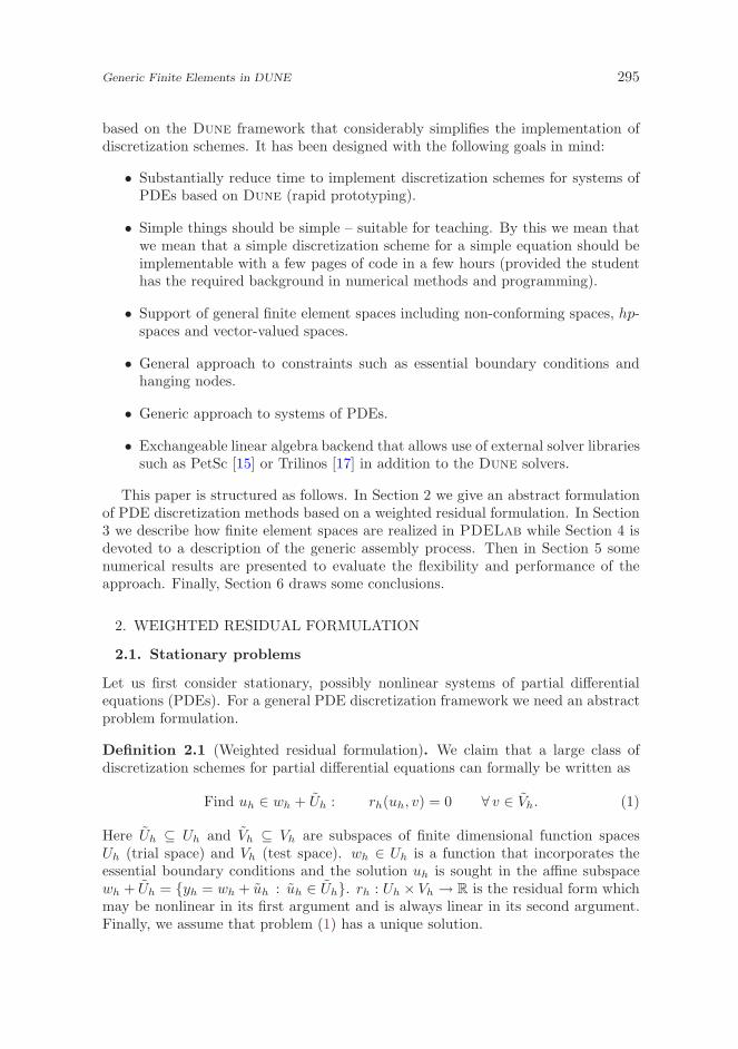
Fig. 1. Assignment of degrees of freedom to entities in the Lagrange basis of P4.

Finally, the third ingredient of the local description of finite element spaces is aclass implementing LocalCoefficientsInterfacewhich assigns degrees of freedomto geometrical entities on the reference element. This allows a generic constructionof the local-to-global map g(T, i) in Definition 3.1. Consider as an example theLagrange basis of P4 on a triangle as shown in Figure 1 (we consider the two-dimensional case for ease of presentation). It has 15 degrees of freedom, threelocated in the element (codimension 0), three located in each edge (codimension 1)and one in each vertex (codimension 2). The assignment of each degree of freedomis encoded as a triple (s, c, i) where s is the number of the geometrical entity (thenumbering is defined in the Dune grid interface) with codimension c and i is anindex within the entity. Listing all the triples for the P4 Lagrange basis is performedby the following code:

typedef Pk3DLocalCoefficients<4> LocalCoefficients;

LocalCoefficients localcoefficients; for (int i=0;

i<localcoefficients.size(); i++)

std::cout << "degree of freedom " << i << " in "

<< localcoefficients.localKey(i).subEntity() << ","

<< localcoefficients.localKey(i).codim() << ","

<< localcoefficients.localKey(i).index() << ","

<< std::endl;

LocalBasis, LocalInterpolation and LocalCoefficients together make up thelocal description of a finite element and are accessible from a class implementingLocalFiniteElementInterface. In Definition 3.1 every element T ∈ Th can havea different local basis. All local descriptions are collected in a container providingaccess to the local description for a given element T . These containers are called localfinite element maps and implement LocalFiniteElementMapInterface. Genericsetup of the local finite element map for our P4 example for a given gridview objectof type GridView (a part of a Dune grid) is shown here:

typedef GridView::ctype D; // coordinate type typedef double R;

302 P. BASTIAN, F. HEIMANN AND S. MARNACH

// value type typedef Pk3DLocalFiniteElementMap<GridView,D,R,4>

LFEM; LFEM lfem(gridview);

In an hp-version of the finite element method the local finite element map would storethe polynomial degree per element and deliver the appropriate local description.

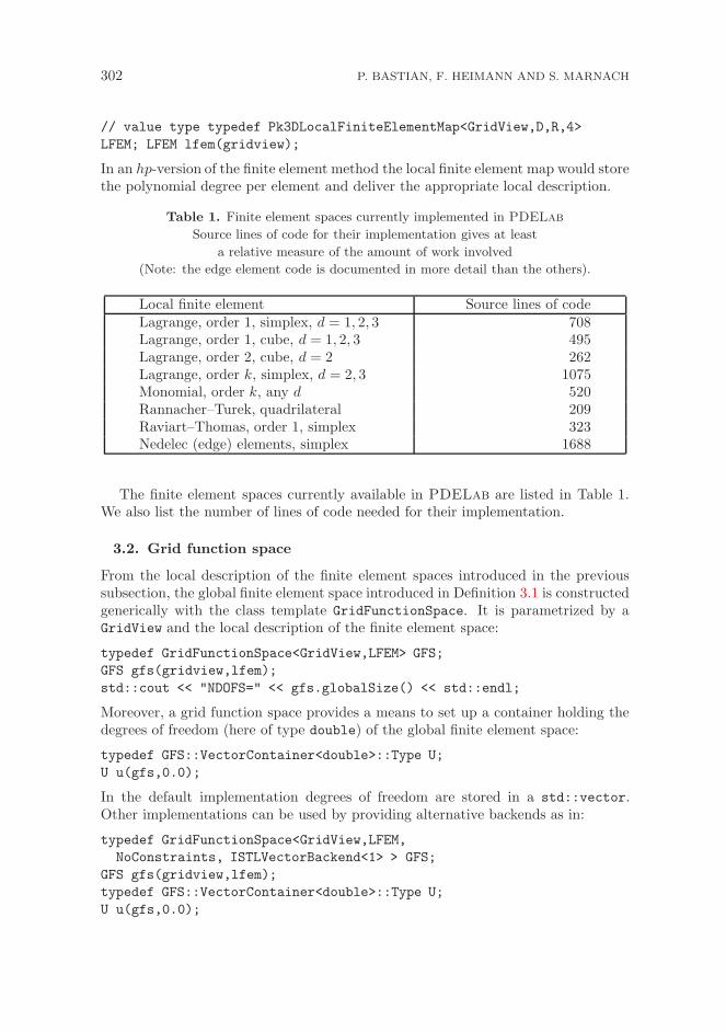
Table 1. Finite element spaces currently implemented in PDELab

Source lines of code for their implementation gives at least

a relative measure of the amount of work involved

(Note: the edge element code is documented in more detail than the others).

Local finite element Source lines of codeLagrange, order 1, simplex, d = 1, 2, 3 708Lagrange, order 1, cube, d = 1, 2, 3 495Lagrange, order 2, cube, d = 2 262Lagrange, order k, simplex, d = 2, 3 1075Monomial, order k, any d 520Rannacher–Turek, quadrilateral 209Raviart–Thomas, order 1, simplex 323Nedelec (edge) elements, simplex 1688

The finite element spaces currently available in PDELab are listed in Table 1.We also list the number of lines of code needed for their implementation.

3.2. Grid function space

From the local description of the finite element spaces introduced in the previoussubsection, the global finite element space introduced in Definition 3.1 is constructedgenerically with the class template GridFunctionSpace. It is parametrized by aGridView and the local description of the finite element space:

typedef GridFunctionSpace<GridView,LFEM> GFS;

GFS gfs(gridview,lfem);

std::cout << "NDOFS=" << gfs.globalSize() << std::endl;

Moreover, a grid function space provides a means to set up a container holding thedegrees of freedom (here of type double) of the global finite element space:

typedef GFS::VectorContainer<double>::Type U;

U u(gfs,0.0);

In the default implementation degrees of freedom are stored in a std::vector.Other implementations can be used by providing alternative backends as in:

typedef GridFunctionSpace<GridView,LFEM,

NoConstraints, ISTLVectorBackend<1> > GFS;

GFS gfs(gridview,lfem);

typedef GFS::VectorContainer<double>::Type U;

U u(gfs,0.0);

Generic Finite Elements in DUNE 303

0 0

10

0 0

01

0 1

00

112

012

12 0

00

12 0

00

0 0

00

vj

vk

vi

vm

vn

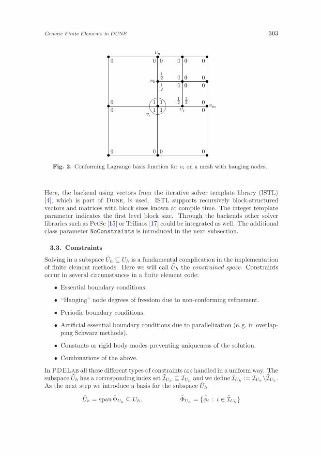
Fig. 2. Conforming Lagrange basis function for vi on a mesh with hanging nodes.

Here, the backend using vectors from the iterative solver template library (ISTL)[4], which is part of Dune, is used. ISTL supports recursively block-structuredvectors and matrices with block sizes known at compile time. The integer templateparameter indicates the first level block size. Through the backends other solverlibraries such as PetSc [15] or Trilinos [17] could be integrated as well. The additionalclass parameter NoConstraints is introduced in the next subsection.

3.3. Constraints

Solving in a subspace Uh ⊆ Uh is a fundamental complication in the implementationof finite element methods. Here we will call Uh the constrained space. Constraintsoccur in several circumstances in a finite element code:

• Essential boundary conditions.

• “Hanging” node degrees of freedom due to non-conforming refinement.

• Periodic boundary conditions.

• Artificial essential boundary conditions due to parallelization (e. g. in overlap-ping Schwarz methods).

• Constants or rigid body modes preventing uniqueness of the solution.

• Combinations of the above.

In PDELab all these different types of constraints are handled in a uniform way. Thesubspace Uh has a corresponding index set IUh

⊆ IUhand we define IUh

:= IUh\IUh

.As the next step we introduce a basis for the subspace Uh

Uh = span ΦUh⊆ Uh, ΦUh

= φi : i ∈ IUh

304 P. BASTIAN, F. HEIMANN AND S. MARNACH

and assume that it is related to the original basis ΦUhof Uh in the following way:

φi = φi +∑

j∈IUh

(

TUh

)

i,jφj , i ∈ IUh

. (7)

The matrix TUhis sparse and can be assembled locally element by element (with

rigid body modes and periodic boundary conditions as exceptions). For a particularfunction space a class providing the local constraints needs to be given as a templateparameter to the GridFunctionSpace. If no constraints are to be put on the functionspace then NoConstraints is given as a parameter.

Example 3.2 (Hanging nodes). Consider the case of nonconforming refinementand bilinear conforming Lagrange basis functions on the mesh shown in Figure 2.Assume that vm is the only vertex where a Dirichlet boundary condition is applied.Then IUh

= k, j,m, IUh= IUh

\ IUhand

φi = φi +1

2φk +

1

2φj , φn = φn +

1

2φk, φl = φl l 6= i, n.

Using the basis we can now represent functions in the subspace as FEΦh(u) =

∑

i∈IUh

uiφi with u ∈ U = RIU

h . Due to the basis transformation (7) we have the

relationFEΦh

(u) = FEΦh(ST

Uhu) (8)

with the rectangular block matrix

SUh=

(

I TUh

)

. (9)

Here we have assumed that the indices in IUhare ordered such that all indices in

IUhare smaller than those in IUh

. Note that the test space Vh is decomposed in asimilar way in case it is different from the trial space.

3.4. Systems of PDEs

For systems of PDEs we need products of function spaces, as has been illustrated in

Example 2.5. Formally, given m > 1 function spaces U(0)h , . . . , U

(m−1)h we define the

composite function space

Uh = U(0)h × U

(1)h × . . .× U

(m−1)h . (10)

If all component spaces are the same, we can also write

Uh = V mh . (11)

This can be done recursively leading to a tree structure of discrete function spaces.As an example consider the Taylor-Hood element for solving the Stokes equations

which we can write in d space dimensions as

UTHh =

(

U2h

)d× U1

h ,

Generic Finite Elements in DUNE 305

meaning that each velocity component is piecewise quadratic and the pressure ispiecewise linear. To construct such a function space in PDELab we first make twogrid function spaces for velocity components and pressure:

typedef GridView::ctype D; // coordinate type

typedef double R; // value type

typedef Pk3DLocalFiniteElementMap<GridView,D,R,1> P1LFEM;

typedef Pk3DLocalFiniteElementMap<GridView,D,R,2> P2LFEM;

P1LFEM p1lfem(gridview);

P2LFEM p2lfem(gridview);

typedef GridFunctionSpace<GridView,P1LFEM> P1GFS;

typedef GridFunctionSpace<GridView,P2LFEM> P2GFS;

P1GFS p1gfs(gridview,p1lfem);

P2GFS p2gfs(gridview,p2lfem);

Now the class template PowerGridFunctionSpace produces a new grid functionspace out of a compile-time given number of grid function spaces of the same type:

const int dim=GridView::Grid::dimension;

typedef PowerGridFunctionSpace<P2GFS,dim> VGFS;

VGFS vgfs(p2gfs);

Using class template CompositeGridFunctionSpace one can make a new grid func-tion space from given grid function spaces of different types:

typedef CompositeGridFunctionSpace<

GridFunctionSpaceLexicographicMapper,

VGFS,P1GFS> THGFS;

THGFS thgfs(vgfs,p1gfs); // the Taylor--Hood space

The template parameter GridFunctionSpaceLexicographicMapper indicates thatthe degrees of freedom are concatenated in the order given. This is also the defaultin the power version. If all component spaces have the same size, a cyclic numberingcan be selected as well. The new grid function space can be used as before. E.g. thefollowing code instantiates a random access container holding all degrees of freedom:

typedef THGFS::VectorContainer<R>::Type X;

X x(thgfs,0.0);

The tree structure of the grid function space is encoded in its recursive type. Usingtemplate metaprogramming [18] one can iterate over the constituents of the gridfunction space.

3.5. Parallelization support

The Dune grid interface provides support for two parallelization models: nonover-lapping and overlapping. The grid function space provides means for the exchangeof degrees of freedom stored in more than one process. The exchange mechanism

306 P. BASTIAN, F. HEIMANN AND S. MARNACH

can be parametrized in a flexible way with respect to which data is exchanged, whatdata is sent and what is done when data is received.

When the iterative solver template library is used as a solver, certain types ofsolvers such as overlapping Schwarz methods or Krylov subspace methods (CG,BiCGStab, GMRES) can be used without any additional programming effort. Pre-conditioners on nonoverlapping grids are not yet available in a generic way.

4. GRID OPERATORS

4.1. Algebraic form of the constrained problem

We now come back to the solution of the weighted residual problem introduced in(1) which reads:

find uh ∈ wh + Uh : rh(uh, v) = 0 ∀ v ∈ Vh.

To solve it, we introduce the basis representation of the subspaces from Section 3.3and the equivalent problem in terms of coefficients:

find u ∈ U : rh(FEΦh(w) + FEΦh

(u), ψi) = 0 ∀ i ∈ IVh. (12)

Employing the residual map introduced in (3) and the matrices SUh, SVh

from (9)this is then equivalent to the solution of the nonlinear algebraic system

find u ∈ U : SVhR(w + ST

Uhu) = 0. (13)

It is important to note that the residual map R, in part to be provided by the user,is evaluated with respect to the original basis Φh, Ψh which does not involve theconstraints!

4.2. Newton’s method

The nonlinear algebraic system (13) is now solved with Newton’s method. To thatend assume that some approximate solution uk is available. We seek an update zk

such that the next iterate uk+1 = uk + zk is an improved approximation. Lineariza-tion of the equation SVh

R(w + STUh

uk+1) = 0 yields an equation for the update:

SVhR(w + ST

Uhuk) + SVh

∇R(w + STUh

uk)STUh

zk = 0

where we introduced the Jacobian ∇R of the nonlinear map R. Together this resultsin the iteration

uk+1 = uk −(

SVh∇R(w + ST

Uhuk)ST

Uh

)−1SVh

R(w + STUh

uk). (14)

In this iteration scheme the solution vector u contains coefficients with respect tothe transformed basis Φh. Multiplication of (14) with ST

Uhfrom the left and addition

of w on both sides yields

w + STUh

uk+1 = w + STUh

uk − STUh

(

SVh∇R(w + ST

Uhuk)ST

Uh

)−1SVh

R(w + STUh

uk)

Generic Finite Elements in DUNE 307

where we can now set uk := w + STUh

uk to get the final form of the nonlineariteration:

uk+1 = uk − STUh

(

SVh∇R(uk)ST

Uh

)−1SVh

R(uk). (15)

Note that (15) is now an iteration where the solution u is computed with respectto the original basis Φh. The residual evaluation R(uk) and the evaluation of theJacobian ∇R(uk) are also with respect to the original basis and are identical tothe unconstrained case. Thus the incorporation of the constraints can be done in acompletely generic way by the PDELab framework. The algorithmic formulationof the Newton scheme is given as follows:

Algorithm 4.1 (Newton’s method for constrained problem). Let the initial guessu0 with FEΦU

h(u0) ∈ wh + Uh be given. Iterate until convergence

1. Compute residual: rk = R(

uk)

.

2. Transform residual: rk = SVhrk.

3. Solve the update equation in the transformed basis:

(

SVh∇R(uk)ST

Uh

)

zk = rk.

4. Transform update to original basis: zk = STUh

zk. (This is where e. g. interpo-lation to hanging nodes is done).

5. Update solution: uk+1 = uk − zk.

4.3. Generic assembler

As has been stated in Observation 2.6 the residual form can be split into contribu-tions from elements, interior faces and boundary faces. Moreover, we can split theresidual form into rh(u, v) = α(u, v) + λ(v) where λ is only allowed to depend onthe test function. The splitting of the residual form rh results into a correspondingsplitting of the nonlinear residual map R and its Jacobian ∇R. The splitting of thenonlinear residual map e. g. reads

R(u) =∑

e∈E0

h

RTe α

volh,e(Reu) +

∑

e∈E0

h

RTe λ

volh,e

+∑

f∈E1

h

RTl(f),r(f)α

skelh,f (Rl(f),r(f)u) +

∑

f∈E1

h

RTl(f),r(f)λ

skelh,f

+∑

b∈B1

h

RTl(b)α

bndh,b (Rl(b)u) +

∑

b∈B1

h

RTl(b)λ

bndh,b ,

where the restriction matrices Rx extract all degrees of freedom related to an ele-ment, interior face or boundary face which can be easily determined from the local-to-global map computed in the grid function space.

The implementor of a discretization scheme only has to provide at most the sixmethods α

vol, αskel, α

bnd, λvol, λ

skel and λbnd providing element, interior face and

308 P. BASTIAN, F. HEIMANN AND S. MARNACH

boundary face contributions depending on solution and test functions (α-terms) oronly on the test functions (λ-terms). Contributions to the Jacobian can be generatedthrough numerical differentiation for rapid prototyping. If an analytical Jacobianis required or a modified Newton method is desired additional methods have to beprovided.

From these user given methods assembling of the residual and the Jacobian (stiff-ness matrix) as well as the complete Newton iteration with consideration of all typesof constraints is provided in a completely generic way including parallel computa-tions, with the exception of the preconditioner.

In order to give a code example for the implementation of a discretization schemewe consider the cell-centered finite volume method from example 2.3. The followingclass Laplace implements this method for the pure Neumann problem on axiparallelcube meshes in any dimension:

template<typename Real> class Laplace : public

NumericalJacobianApplySkeleton<Laplace<Real> >,

public NumericalJacobianSkeleton<Laplace<Real> >,

public FullSkeletonPattern, public FullVolumePattern,

public LocalOperatorDefaultFlags

public:

// pattern assembly flags

enum doPatternVolume = true ; enum doPatternSkeleton = true ;

// residual assembly flags

enum doAlphaSkeleton = true ;

template<typename IG, typename LFSU, typename X, typename LFSV, typename R>

void alpha_skeleton (const IG& ig,

const LFSU& lfsu_s, const X& x_s, const LFSV& lfsv_s,

const LFSU& lfsu_n, const X& x_n, const LFSV& lfsv_n,

R& r_s, R& r_n) const

// face volume for integration

Real face_volume = ig.geometry().volume();

// cell centers in global coordinates

Dune::FieldVector<Real,IG::dimension>

inside_global = ig.inside()->geometry().center();

Dune::FieldVector<Real,IG::dimension>

outside_global = ig.outside()->geometry().center();

// distance between the two cell centers

inside_global -= outside_global;

Real distance = inside_global.two_norm();

// contribution to residual on inside element

r_s[0] += (x_s[0]-x_n[0])*face_volume/distance;

r_n[0] -= (x_s[0]-x_n[0])*face_volume/distance;

;

Generic Finite Elements in DUNE 309

Table 2. Coding effort required to implement various

discretization schemes for an elliptic model problem.

Method Source lines of codeConforming finite elements 298Discontinuous Galerkin 914Cell-centered finite volumes 222Mixed finite elements 288Mimetic finite differences 395

In that case only one term in (5), the interior skeleton term αskel is needed which

is implemented in the method alpha skeleton. This also illustrates the fact thatsimple methods can be implemented with very few lines of code which makes thesystem usable for teaching.

5. NUMERICAL RESULTS

In this Section we present some applications of the PDELab framework in order todemonstrate its flexibility and performance.

5.1. Six easy pieces

The elliptic problem (4) with tensor diffusion coefficient and Dirichlet as well asNeumann boundary conditions can be solved with the following methods:

• Conforming finite elements (arbitrary order for simplices and d = 2, 3, order 1and 2 for hexahedral elements in d = 2, 3, hanging nodes for order 1).

• Discontinuous Galerkin finite elements (Oden–Babuska–Baumann, symmetricinterior penalty method, nonsymmetric interior penalty method).

• Nonconforming Rannacher–Turek element in d = 2.

• Lowest order Raviart–Thomas (mixed) elements on triangles (non-hybrid ver-sion).

• Cell-centered finite volumes with harmonic permeability averaging (scalar dif-fusion coefficient only) in any dimension on axi-parallel hexahedral meshes.

• Mimetic finite difference method [6] on any mesh in any dimension.

Table 2 lists the number of lines of code required to implement the various dis-cretization schemes in PDELab. It should be noted that all schemes, except thecell-centered finite volumes and lowest-order mixed method, implement also the an-alytical Jacobian. The table shows that all schemes can be implemented with a verylow effort. Note also that this table does not include the source lines required toimplement the function spaces. These are given in Table 1.

310 P. BASTIAN, F. HEIMANN AND S. MARNACH

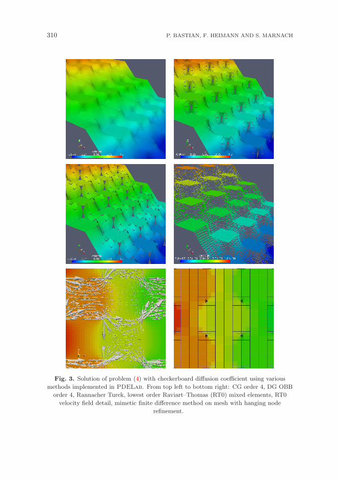
Fig. 3. Solution of problem (4) with checkerboard diffusion coefficient using various

methods implemented in PDELab. From top left to bottom right: CG order 4, DG OBB

order 4, Rannacher Turek, lowest order Raviart–Thomas (RT0) mixed elements, RT0

velocity field detail, mimetic finite difference method on mesh with hanging node

refinement.

Generic Finite Elements in DUNE 311

Figure 3 shows visualizations of the results obtained with the different schemesapplied to a model problem with a checker-board coefficient distribution in two spacedimensions.

5.2. Multiphase flow in porous media

In order to demonstrate the suitability of PDELab for a more complicated problem,we solve the problem of two-phase immiscible flow in porous media, see e. g. [11]for an introduction. The phases considered are liquid (l) and gas (g) and the modelconsists of conservation of mass for each phase α ∈ l, g:

∂t(φsανα) + ∇ · ναuα = qα,

where sα is the phase saturation, να is the molar density, uα is the phase velocityand qα is the source/sink term. The phase velocity depends on the pressure via theextended Darcy law

uα = −krα(sα)

µα

K (∇pα − ραg) ,

where the relative permeability krα depends nonlinearly on saturation, K is theabsolute permeability, µα is the dynamic viscosity of the fluid, ρα is the mass densityof the fluid and g is the gravity vector. In addition there are the following algebraicconstraints for saturations and pressures:

sl + sg = 1 pl + pg = pc(sl),

where pc(sl) is the strongly nonlinear capillary pressure saturation relation. Finally,for the gas phase we have the ideal gas law νg = pg/RT and for the liquid phaseνl = const.

This system is solved in a so-called pressure-pressure formulation which amountsto a time-dependent, strongly nonlinear system of two coupled PDEs which is dis-cretized using a cell-centered finite-volume scheme with harmonic averaging of per-meabilities and upwinding of mobilities. In time, a fully-implicit Euler scheme isused. The resulting nonlinear algebraic system per time step is solved using New-ton’s method with line search globalization and the arising linear systems are solvedwith a BiCGStab Krylov subspace method with an overlapping inexact Schwarzpreconditioner using a few steps of Block-SSOR as subdomain solver.

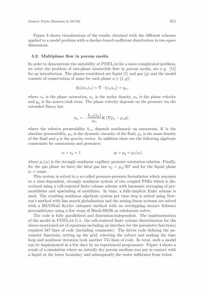
The code is fully parallelized and dimension-independent. The implementationof the model in PDELab (i. e. the cell-centered finite volume discretization for theabove-mentioned set of equations including an interface for the parameter functions)required 587 lines of code (including comments). The driver code defining the pa-rameter functions, setting up the grid, selecting the solvers and making the timeloop and nonlinear iteration took another 755 lines of code. In total, such a modelcan be implemented in a few days by an experienced programmer. Figure 4 shows aresult of a simulation where an initially dry porous medium was put in contact witha liquid at the lower boundary and subsequently the water infiltrates from below.

312 P. BASTIAN, F. HEIMANN AND S. MARNACH

Fig. 4. Capillary rise of a fluid in a hele-shaw cell containing a coarse sand. Left image

shows liquid phase pressure, right image shows contours of liquid phase saturation.

Nowadays multi-core CPUs are standard for various technical reasons. A majorproblem in using such CPUs for scientific computing is the limited memory band-width when all cores access main memory. Table 3 gives some performance numbersof Dune and PDELab on such architectures. We use a system with four quad-coreAMD Opteron 8380 processors (2.5 GHz). Each core has 512KB L2 cache and allfour cores in a CPU share a 6MB L3 cache. We solve one time step of the two-phase flow problem on a 160 × 160 × 96 grid resulting in roughly 5 million degreesof freedom. The first two columns give the maximum number of iterations and thecorresponding computation time of the overlapping Schwarz preconditioner (3 cellsoverlap) in any Newton step. Iteration numbers are robust with respect to num-ber of processors and the speedup for one iteration (time in fourth column) on 16processors is 9. The time for assembly of the Jacobian (next column) scales slightlybetter. Finally the speedup in total computation time is 8 on 16 processors.

5.3. Parallel solver example

Figure 5 shows results for the scalability of an additive geometric multigrid pre-conditioner, the so-called BPX method [5], implemented in Dune. All multigridcomponents are implemented with sparse linear algebra classes from the iterativesolver template library [1, 4] such that no access to the grid is necessary duringmultigrid cycles. The YaspGrid (a structured, parallel grid) implementation fromdune-grid is used in two space dimensions. Strong scaling means that a 2048×2048problem is solved on one up to 256 processors. The speedup attained on 256 proces-sors is 124, i. e. almost 50% efficiency. In the weak scaling test each processor has a1024× 1024 grid and the problem size is increased proportional with the number of

Generic Finite Elements in DUNE 313

Table 3. Strong scaling for two-phase flow problem of size 160 × 160 × 96

on a 4×quad-core AMD Opteron 8380 system (2.5 GHz).

P #IT(max) Tlin(max) Tit Tass Ttotal Speedup1 40.5 264.5 6.5 39.2 1347.3 -2 44.5 138.5 3.2 31.1 810.5 1.74 44.5 71.2 1.6 16.1 407.8 3.38 42.5 53.3 1.3 7.7 279.5 4.8

16 50.0 34.4 0.7 3.8 163.1 8.2

1

10

100

1 10 100

Spee

dup

Processors

idealstrong scalingweak scaling

Fig. 5. Strong and weak scalability of an additive geometric multigrid preconditioner

using YaspGrid on a Linux cluster (dual processor dual core AMD Opteron 2.8 GHz,

Myrinet 10GBit interconnect).

processors. In this mode a speedup of 163 is achieved on 256 processors.

6. CONCLUSIONS

In this paper we presented software abstractions for the generic implementationof finite element methods. The system allows a very general definition of finiteelement spaces including higher order, continuous and discontinuous as well as scalarand vector-valued. Moreover, a general way for the incorporation of constraints isprovided. In the examples it is shown that many schemes can be implemented witha low programming effort with the underlying Dune framework providing dimensionindependence and parallelization. Learning how to use a system like PDELab takesa certain amount of time which strongly depends on the background and experienceof the user. However, as soon as features like higher-order or parallelism are requiredthis initial investment should pay off.

The current state of implementation of PDELab encompasses the global finite

314 P. BASTIAN, F. HEIMANN AND S. MARNACH

element spaces described in Section 3, including constraints and generic parallelism.The generic assembler for stationary problems and the Newton scheme are imple-mented as well. As the next steps generic support for adaptivity and time dependentproblems will be integrated into PDELab.

ACKNOWLEDGEMENT

We wish to thank all Dune developers for their effort and support, Christoph Gruningerfor the provision of the DG code, Jo Fahlke for the implementation of several finite elementspaces. The support of StatoilHydro for the Dune project is also greatly acknowledged.

(Received March 3, 2010)

R EF ERENC ES

[1] P. Bastian and M. Blatt: On the generic parallelisation of iterative solvers for thefinite element method. Internat. J. Comput. Sci. Engrg. 4 (2008), 1, 56–69.

[2] P. Bastian, M. Blatt, A. Dedner, C. Engwer, R. Klofkorn, M. Ohlberger, andO. Sander: A generic grid interface for parallel and adaptive scientific computing.Part I: Abstract framework. Computing 82 (2008), 2-3, 103–119.

[3] P. Bastian, M. Blatt, A. Dedner, C. Engwer, R. Klofkorn, R. Kornhuber,M. Ohlberger, and O. Sander: A generic grid interface for parallel and adaptivescientific computing. Part II: Implementation and tests in DUNE. Computing 82

(2008), 2-3, 121–138.

[4] M. Blatt and P. Bastian: The iterative solver template library. In: Applied ParallelComputing. State of the Art in Scientific Computing (B. Kagstrum, E. Elmroth,J. Dongarra, and J. Wasniewski, eds.) (Lecture Notes in Sci. Comput. 4699.) Spinger,Berlin 2007, pp. 666–675.

[5] J.H. Bramble, J. E. Pasciak, and J. Xu: Parallel multilevel preconditioners. Math.Comput. 55 (1990), 1–22.

[6] F. Brezzi, K. Lipnikov, and V. Simoncini: A family of mimetic finite differencemethods on polygonal and polyhedral meshes. Math. Models and Methods in AppliedSciences 15 (2005), 10, 1533–1551.

[7] P.G. Ciarlet: The Finite Element Method for Elliptic Problems. SIAM, Philadelphia2002.

[8] A. Dedner, R. Klofkorn, M. Nolte, and M. Ohlberger: A generic interface for paralleland adaptive scientific computing: Abstraction principles and the Dune-Fem mod-ule. Preprint No. 3, Mathematisches Institut, Universitat Freiburg, 2009. Submittedto Transactions on Mathematical Software.

[9] http://www.dune-project.org/, Dune Homepage, link visited August 3, 2009.

[10] C. Geuzaine and J.-F. Remacle: Gmsh: A 3-d finite element mesh generator withbuilt-in pre- and post-processing facilities. Internat. J. Num. Methods in Eng., 2009.http://www.geuz.org/gmsh/, link visited August 3, 2009.

[11] R. Helmig: Multiphase Flow and Transport Processes in the Subsurface – A Contri-bution to the Modeling of Hydrosystems. Springer–Verlag, 1997.

Generic Finite Elements in DUNE 315

[12] J. T. Oden, I. Babuska, and C. E. Baumann: A discontinuous hp finite elementmethod for diffusion problems. J. Comput. Phys. 146 (1998), 491–519.

[13] http://www.opencascade.com/, link visited August 3, 2009.

[14] http://www.paraview.org/, link visited August 3, 2009.

[15] http://www.mcs.anl.gov/petsc/petsc-as/ , link visited August 5, 2009.

[16] http://www.salome-platform.org/, link visited August 3, 2009.

[17] http://trilinos.sandia.gov/, link visited August 5, 2009.

[18] D. Vandevoorde and N.M. Josuttis: C++ Templates – The Complete Guide.Addison-Wesley, 2003.

Peter Bastian, IWR, Im Neuenheimer Feld 368, D-69120 Heidelberg. Germany.

e-mail: peter.bastian@iwr.uni-heidelberg.de

Felix Heimann, IWR, Im Neuenheimer Feld 368, D-69120 Heidelberg. Germany.

e-mail: felix.heimann@iwr.uni-heidelberg.de

Sven Marnach, IWR, Im Neuenheimer Feld 368, D-69120 Heidelberg. Germany.

e-mail: sven.marnach@iwr.uni-heidelberg.de