Generational Trends in Vehicle Ownership and Use: Are Millennials Any Different?christopher R. Knittel and Elizabeth Murphy

M A S S A C H U S E T T S I N S T I T U T E O F T E C H N O L O G Y

April 2019 CEEPR WP 2019-006

Working Paper Series

Generational Trends in Vehicle Ownership and Use: Are Millennials

Any Different?

Christopher R. Knittel and Elizabeth Murphy∗

February 8, 2018

Abstract

Anecdotes that Millennials fundamentally differ from prior generations are numerous in thepopular press. One claim is that Millennials, happy to rely on public transit or ride-hailing, areless likely to own vehicles and travel less in personal vehicles than previous generations. How-ever, in this discussion it is unclear whether these perceived differences are driven by changesin preferences or the impact of forces beyond the control of Millennials, such as the Great Re-cession. We empirically test whether Millennials’ vehicle ownership and use preferences differfrom those of previous generations using data from the US National Household Travel Survey,Census, and American Community Survey. We estimate both regression and nearest-neighbormatching models to control for the confounding effect of demographic and macroeconomic vari-ables. We find little difference in preferences for vehicle ownership between Millennials andprior generations once we control for confounding variables. In contrast to the anecdotes, wefind higher usage in terms of vehicle miles traveled (VMT) compared to Baby Boomers. Nextwe test whether Millennials are altering endogenous life choices that may, themselves, affectvehicles ownership and use. We find that Millennials are more likely to live in urban settingsand less likely to marry by age 35, but tend to have larger families, controlling for age. On net,these other choices have a small effect on vehicle ownership, reducing the number of vehiclesper household by less than one percent.

Keywords: Vehicle ownership, vehicle miles traveled, Millennials, Demographic ShiftsJEL Codes: R2, O18, L9

∗Knittel: George P. Shultz Professor Sloan School of Management and Director Center for Energy and Environmen-tal Policy Research, MIT and NBER, knittel@mit.edu; Murphy: Genser Energy, elizabeth.murphy330@gmail.com. We thank seminar participants at MIT and UC Berkeley. Emil Dimanchev and Randall Field gave valuable feedback.

1 Introduction

The Millennial generation is often thought to be upsetting institutional and economic norms

established by previous generations. From differences in fast-food eating preferences to changes in

the investments they make, the common consensus is that Millennials are fundamentally disrupting

a wide variety of industries due to differences in preferences. However, such claims have not been

explored rigorously, and limited data have been used to support these hypotheses.1

Understanding the true preferences of the Millennial generation, as well as the demographic

makeup of the generation, can provide insight into the future landscape of mobility, and thus

provide both the industry and policy makers with more information about what business practices

and policies to implement. This paper empirically tests whether Millennials’ vehicle decisions

differ from those of previous generations. Our focus is on two main facets of personal mobility:

vehicle ownership, measured by how many vehicles a given household owns, and vehicle usage,

measured by annual vehicle miles traveled (VMT). Each of these provides different insights; vehicle

ownership gives a better understanding of the market for personal vehicles, while vehicle miles

traveled provides insight on vehicle fleet usage as well as environmental footprints.

Our data come from Department of Transportation’s National Household Transportation Survey

and the US Census and the American Community Survey to construct a picture of both transport

preferences and generational demographics. Our goal is to tease apart two primary factors that

could account for the changes in vehicle purchasing and use: preferences for transportation con-

ditional on demographics and differences in endogenous household demographics (e.g., marriage)

themselves and how these decisions indirectly affect transportation choices.

The first of our goals captures the shift in preferences holding constant other factors that

influence vehicle ownership and use with the goal to understand whether observed differences are

due to differences in other variables that might influence transportation decisions. The second

seeks to understand how much endogenous changes in life choices, such as marriage and urbanity,

influence vehicle ownership and use. We refer to these effects as indirect. To measure these we also

estimate the degree to which Millennials are altering these other endogenous decisions and, through

our empirical model of transportation decisions conditional on these other factors, measure how

these changes affect ultimate transportation demand.

Our work adds a rigorous analysis of Millennial preferences to a discussion that is dominated

by anecdotal evidence for perceived differences in purchasing and use habits, with claims that

Millennials are the “go nowhere generation” meaning they are more risk averse and less mobile

Buchholz and Buchholz (2012), or the “cheapest generation,” who are not interested in making

large investments in cars or houses Thompson and Weissman (September 2012 Issue). We find

that, conditional on household demographics, Millennials do not differ in terms of vehicle ownership,

relative to Baby Boomers. In addition, Millennial vehicle use, measured by annual vehicle miles

traveled (VMT) is higher than Baby Boomers at similar stages in their lives. The net effect, however,

1See, for example, Taylor (2017),Dutzik et al. (2014) and Fry (2017).

1

is a bit more nuanced. We also find that Millennials are delaying some of the life choices that are

held constant in the preceding statements. Together, the results suggest that while Millennial

vehicle ownership and use may be lower early on in life, these differences are only temporary and,

in fact, lifetime vehicle use is likely to be greater.

Two concurrent papers complement our results using different methodologies. Leard et al.

(2019) uses pre-Great Recession NHTS data to estimate how VMT responds to changes in demo-

graphics and then compares the forecasts of this relationship to observed VMT. They find that

economic factors can explain most the variation in VMT, leaving little room for generational dif-

ferences to explain movements in VMT. Our work directly tests for generational differences using

the 2017 NHTS sample, a year where Millennials were in their early- to mid-30s. We also estimate

how Millennials might be changing life choices and the impact these have on vehicle ownership.

Kurz et al. (2018) uses consumer expenditure data to estimate whether Millennials are spending

any less on vehicles and shows Millennials’ spending is inline with previous generations. We do not

focus on spending.

The remainder of the paper proceeds as follows. In Section 2 we discuss the data used in

the analysis. Section 3 discusses the empirical models and results for estimating the change in

preference, conditional on demographics. Section 4 estimates how Millennials differ in terms of other

life choices and what these differences imply for vehicle ownership. Finally, Section 5 concludes.

2 Data Souces

Our primary data source is the Department of Transportation’s National Household Travel

Survey (NHTS). We utilize surveys from 1990, 1995, 2001, 2009, and 2017.2 We also make use of

data from the US Census and American Community Survey (ACS). Both the Census and American

Community Survey data used in this analysis are provided by the Integrated Public Use Microdata

Series compiled by the University of Minnesota. Data from Census years 1990, 2000, and 2010

are included in the analysis, as well as the American Community Survey from 2015, an off-cycle

year for the US Census. The three data sets contain responses at the person- and household-level;

however, they differ somewhat in the demographic variables they collect within a household. We

also use the Census data to analyze other life choices.

We analyze vehicle ownership at the household-level for both datasets, since vehicles are more

often attributed to households rather than individuals—couples typically share the expenses of a

vehicle—and the data sets recorded household identification for the vehicles rather than personal

designation. We focus on VMT at the person level since VMT can be attributed to an individual,

although our general conclusions are robust to aggregate VMT to the household level. Only the

NHTS data contain information on VMT.

Several steps to clean and organize the data were necessary to analyze households decisions.

To assign the appropriate generation to each household, the head of household was identified from

2The 2016 survey spans April 2016 through April 2017. It will be referred to as the 2017 survey throughout thiswork.

2

the person-level responses by selecting the eldest member of each family.3 Their birth year was

used to assign a generation to the household based on the delineations in Table 1.4 Lastly, any

demographic information used in the model is based on the head of household’s characteristics.

Generation Birth Years

Millennials 1980-1994Generation X 1965-1979Baby Boomers 1946-1964Silent Generation 1928-1945Greatest Generation 1901-1927

Table 1: Generation assignments for households in the United States

3 Vehicle Ownership and Use, Conditional on Demographics

3.1 Empirical Set Up

Our basic approach is to use linear regression to control for household and time characteristics.

We also test the robustness of these results using a nearest-neighbor matching model that matches

on the same demographics and control variables as in the regressions.

For much of our analysis, we restrict ourselves to only the most recent three generations: Baby

Boomers, Generation X, and Millennials, using Baby Boomers as the omitted category (baseline

generation). We relate the variables of interest (e.g., vehicles per household or VMT) to the

generation controlling for confounders. Specifically we have:

yit = β0 + β1IMilli + β2I

GenXi +Xitγ + εit, (1)

where Igi are indicators for the generation that the head of household of household i falls into, Xit

are household level demographics and time control variables, and εit is the regression residual. We

estimate a variety of models varying the control variables. Our list of complete control variables

is in Table 2. For each of the continuous variables, we include its natural log in the regression

and the square of the natural log of the variable to account for non-linearities in the relationship.

We cluster our standard errors at the state level allowing for arbitrary correlation in the residuals

across households within the same state.

3The risk here is if an elderly parent is living in the household. We have also performed the analysis where wedefine the generation based on the second oldest adult if that adult is older than 30 and the gap between the secondoldest and the oldest is at least 18 years. This is meant to capture cases where the child is the head of household.We note that this is not an issue for the Census data, described below, because it explicitly asks for the age of thehead of household.

4These assignments reflect those used by the Pew Research Center in their demographics analysis and reporting.

3

Table 2: Demographic variables included in models

Control Variables

IncomeHousehold SizeHousehold Composition Effects+,†

Location: Urban v. Rural+

Location: State Fixed EffectsEducationSurvey YearAgeSexRaceFamily Life Cycle†

Marital Status∗

Number of Children∗

Notes: +: The NHTS data contain 10 household composition indicators. These indicate whether thehousehold has 1 or 2 adults working adults, and then either: no children, a youngest child between 0 and5-years old, a youngest child between 6 and 15, and a youngest child between 16 and 21. The final twocategories capture whether there are 1 or 2 or more retired adults with no children. For Urbanity, the NHTSdata have four categories: in an urban area, in an urban cluster, in an area surrounded by urban areas (only72 observations fit this), and not in an urban area. †: Variable available in NHTS data set only. *: Variableavailable in Census/ACS data sets only.

3.2 Results

We begin by showing results with no controls and then add to the set of control variables.

Figure 1 plots the coefficients for the Millennial and Generation X indicators and their respective

95% confidence intervals. Baby Boomers are the omitted category. We estimate seven specifications

in total.

The first model, indicated in the dark blue color, includes data from all households of all ages

18 and older. The regression does not include any demographic controls, therefore representing the

difference in unconditional means. The coefficient for Millennials is strongly negative, indicating

that on average Millennials own approximately 0.4 fewer vehicles per household than the average

Baby Boomer. This model represents the most easily observed trends in vehicle ownership among

Millennials, as vehicle ownership is quantified based solely on what generation a household belongs

to, which fuels the speculation that Millennials are fundamentally different.

The second model differs from the first only in that the baseline controls for demographics

and economic factors are included. The inclusion of these control variables dramatically reduces

the magnitude of the coefficients for each generation; the Millennial coefficient falls from 0.39 to

0.17. This indicates that the underlying endowments of the generations are not consistent across

the generations, as is to be expected, and these endowments are affecting vehicle ownership. This

model is still incomplete as there are weaknesses in how age is controlled.

4

-.4-.3

-.2-.1

0.1

Millennial Gen XCoefficient

All Ages, No Controls All Ages, Baseline Controls Ages 18-37, No Controls

Ages 18-37, Baseline Controls Ages 18-37, No Age Control Ages 18-37, State/Yr Interactions

Ages 18-37, State Macroecon

Regression Models

Figure 1: NHTS vehicle count regression coefficients by generation

One limitation of the data available is that data for Millennials are only available for Millennials

who are a maximum of 37 years old. This arises from the definition of Millennials, whose oldest

members were born in 1980. As a result, although the age variables are included as regressors, the

range of ages across generations do not share the same support. To address this, the remaining

regression models on the plot only include heads of household aged 18-37. These also, by the nature

of the age distributions in the data, omit the Silent and Greatest generations.

The third plot, indicated in green, shows the regression coefficients for the model where only

ages 18-37 are included, and does not include any of the demographic control variables. The results

of this model show an even smaller magnitude coefficient for Millennials (−0.08), emphasizing the

importance of age effects in vehicle ownership.

The fourth plot, in yellow, depicts the results for households aged 18-37 and includes the full

set of demographic variables; this is our preferred specification. The model uses the regressors

and examines the subset of the data for households aged 18-37. The resulting coefficients for

both Millennials and Generation X approach 0, and neither are statistically significant from 0.

The Millennial coefficient is −0.03, while the Generation X coefficient is 0.005. (We cannot reject

equality between the Millennial and Generation X coefficients.) These results support the conclusion

5

that Millennials do not have different preferences from previous generations when both age effects

and endowments are accounted for in vehicle ownership rates.

We also briefly discuss the other coefficients, reported Appendix Table A.1 for our preferred

specification. Given the inclusion of the quadratic terms for the continuous variables, the impact

of control on vehicle ownership is immediately obvious. Therefore, we discuss the distributions of

the derivatives. Each are intuitive. The mean of the derivative with respect to income is 0.29,

with a standard error of 0.023. The minimum value is 0.20, while the maximum value is 0.32. The

mean for the age derivative is 0.18 with a standard error of 0.014. The minimum is 0.13 while

the maximum is 0.20. While it would not be surprising if the derivative did turn negative at some

age level, recall that we are restricting the sample to households where the head is below 38. The

mean for the household derivative is 0.71 while the standard error is 0.49. Here, the derivative

does turn negative for household size larger than 5. While our prior is that the derivative likely

remains positive throughout the household size distribution, given that less than 2.9 percent of

sample has a household size above 5, it is not too surprising that the model has a hard time fitting

these observations.

The variables capturing urbanity also have intuitive signs. The omitted group is living in an

urban area. Living in an urban cluster, thus less urban than the omitted group, is associated with a

0.11 increase in the number of vehicles per household. Living in the surrounding areas of an urban

area is associated with a 0.12 increase, while living in a rural area is associated with a 0.3 increase

in the number of vehicles. Finally, we find that higher education levels are associated with initial

increases in the number of vehicles, but then this effect starts to wane at Bachelor’s degrees and

above, again noting that we are conditioning on other confounders such as income and household

size.

To explore the robustness of the findings, we estimate three additional models specifications

varying how we control for age and the survey year. The fifth plot in light blue shows the results

from a model in which an additional age control variable is no longer included in the regression

equation. The goal of this specification is to understand if a control variable for age is necessary in

addition to sub-setting the data to include only ages 18-37. The results from this specification have

a larger coefficient in magnitude, indicating a difference in preferences for vehicles by Millennials.

This suggests that restricting the sample to only households aged 18-37 does not adequately control

for age. This is not surprising, given that age is estimated to have an important effect on vehicle

ownership the distribution of age differs across generations. For example, the range of ages for

Baby Boomers, which have been defined as those born 1946-1965, does not range from 18-37, but

rather only from ages 26-37 since the oldest data set used is 1990. Therefore, it is important to use

the age control variable since the distribution of Baby Boomers will be different than for that from

Generation X or Millennials.

The sixth plot, in red, increases the flexibility in the survey year fixed effects, meant to capture

macroeconomic activity. Specifically, we include a set of state-by-survey year fixed effects. The

coefficients do not differ considerably from the baseline results plotted in the fourth model. This

6

supports the baseline model’s more simple approach of using only the year variable rather than an

additional interaction term.

The final specification, in purple, explores the macroeconomic effects more quantitatively by

including state macroeconomic data on gross state product and state unemployment rates, rather

than the survey fixed effects. This specification is also partly motivated by the fact that Age and

the set of survey fixed effects are jointly estimated off of functional form assumptions: they cannot

both be non-parametrically identified.5

After including these variables to capture state-level macroeconomic conditions, the generation

results from the model depicted in the final plot in black again show very little difference in the

coefficients as compared to the baseline model in yellow. Therefore, the simpler use of the year

variable is sufficient for capturing macroeconomic effects, as the coefficients hardly change when a

more detailed model is constructed.

These six models together provide a clear picture of what is contributing to the difference

in vehicle ownership rates between Millennials and other generations. There are both significant

age effects and differences in underlying endowments. When these two factors are accounted for,

nearly all the differences between Millennials’ and Baby Boomers’ vehicle ownership rates are

eliminated. Therefore, these results suggest that Millennials’ preferences for vehicle ownership are

not so different from prior generations.

To provide a further check on this conclusion, we estimate similar specifications using the

Census/ ACS data. The difference in study years alters the maximum age of Millennials, limiting

it to 35 rather than 37 given that the most recent study year included in the analysis is 2015.

The other difference is that the Census/ACS data set includes explicit variables on whether the

respondent is married and has children. The results are plotted in Figure 2. The full coefficient

estimates are in Appendix Table A.2.

The models in Figure 2 mirror those from the NHTS results and serve as an effective comparison

to the NHTS results to provide a further check on the robustness of the results. Looking at these

data, very similar results are shown in the trends as compared to the NHTS. The baseline model,

the fourth plot indicated again in yellow, shows a similar result to the NHTS results with a small

negative coefficient, approaching 0. However, unlike in the NHTS data set where the 95% confidence

interval is fairly wide and includes 0, the results for Millennials in ACS is statistically significant

from 0, though the magnitude in that confidence interval is very small. These results provide a

confirmation on the conclusions from NHTS that the difference in preferences between Millennials

and prior generations is not actually large, but rather plays a negligible part in the observed

differences in vehicle ownership rates for Millennials compared to other generations. Both data sets

support the conclusion that the observed differences in Millennials’ ownership rates are primarily

from their different endowments and age effects.

Next we turn to results with respect to vehicle usage. We estimate the same set of specifications

for the NHTS data for vehicle miles traveled. The results from the regressions are depicted in

5We include the log of state-level unemployment and the log of GSP, along with their respective squared terms.

7

-.6-.4

-.20

Millennial Gen XCoefficient

All Ages, No Controls All Ages, Baseline Controls

Ages 18-35, No Controls Ages 18-35, Baseline Controls

Ages 18-35, No Age Control Ages 18-35, State/Yr Interactions

Ages 18-35, State Macroecon

Regression Models

Figure 2: Census/ACS vehicle count regression coefficients by generation

Figure 3; the full results are reported in Appendix Table A.3. The same seven regression models

as constructed for the vehicle ownership regressions were done, with the only difference being the

dependent variable. Examining the results, Millennials again appear to be very different from Baby

Boomers when neither age effects nor demographics are included, which corresponds to the model

in blue labeled “All Ages, No Controls.” These results show nearly 2000 fewer miles driven by

Millennials as compared to Baby Boomers. When the control variables are included in the “All

Ages, Baseline Controls” model, the negative coefficient between Millennials and prior generations

disappears, and the result is no statistically significant difference between Millennials and Baby

Boomers.

Interestingly, the model that subsets the data to only include households aged 18-37, with-

out any variable controls, the difference between Millennials and Baby Boomers is actually more

pronounced. This large difference dissipates again when the control variables are included. This

result is interesting as it appears the age effects between Millennials and Baby Boomers are not a

considerable contribution to observed differences between the two generations. Rather, the bulk of

the difference arises from the differences in endowments. When these endowments are accounted

for via the control variables, the coefficient flips to being positive, indicating that in reality Mil-

8

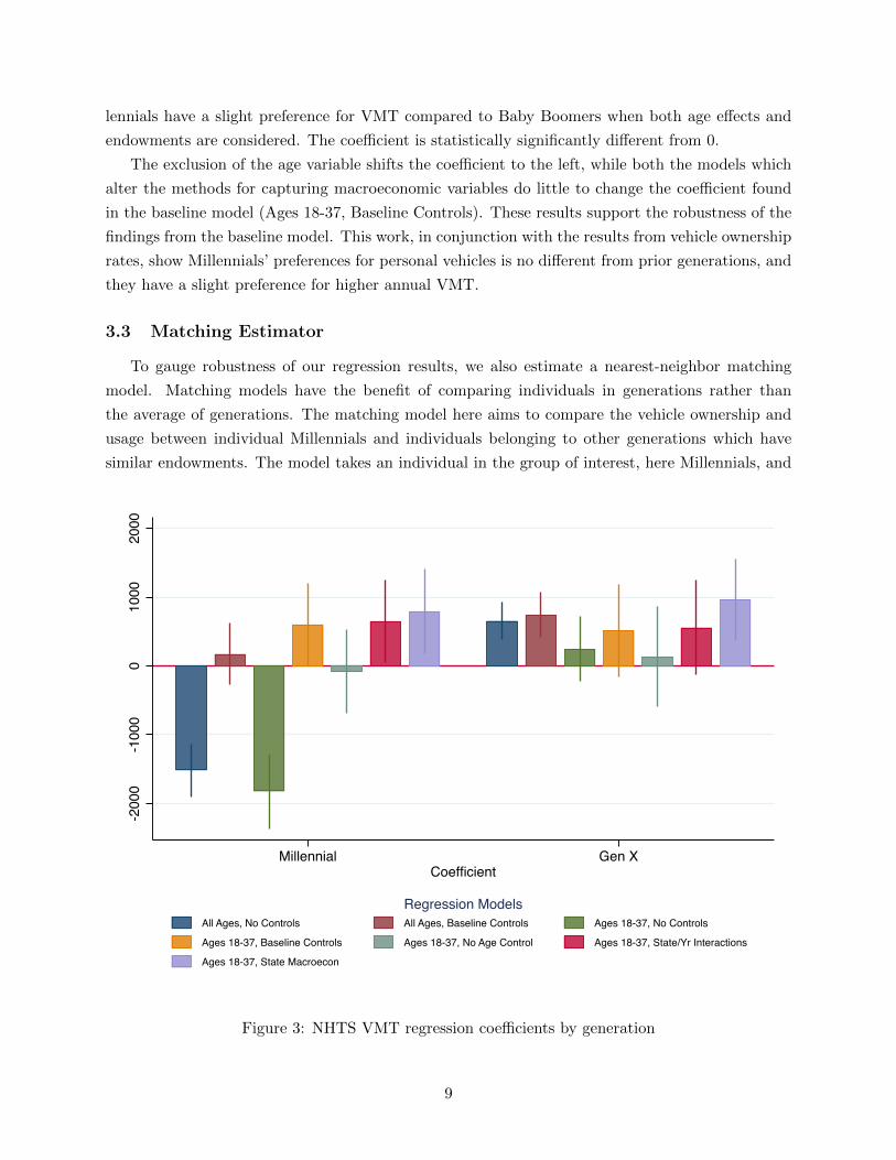
lennials have a slight preference for VMT compared to Baby Boomers when both age effects and

endowments are considered. The coefficient is statistically significantly different from 0.

The exclusion of the age variable shifts the coefficient to the left, while both the models which

alter the methods for capturing macroeconomic variables do little to change the coefficient found

in the baseline model (Ages 18-37, Baseline Controls). These results support the robustness of the

findings from the baseline model. This work, in conjunction with the results from vehicle ownership

rates, show Millennials’ preferences for personal vehicles is no different from prior generations, and

they have a slight preference for higher annual VMT.

3.3 Matching Estimator

To gauge robustness of our regression results, we also estimate a nearest-neighbor matching

model. Matching models have the benefit of comparing individuals in generations rather than

the average of generations. The matching model here aims to compare the vehicle ownership and

usage between individual Millennials and individuals belonging to other generations which have

similar endowments. The model takes an individual in the group of interest, here Millennials, and

-200

0-1

000

010

0020

00

Millennial Gen XCoefficient

All Ages, No Controls All Ages, Baseline Controls Ages 18-37, No Controls

Ages 18-37, Baseline Controls Ages 18-37, No Age Control Ages 18-37, State/Yr Interactions

Ages 18-37, State Macroecon

Regression Models

Figure 3: NHTS VMT regression coefficients by generation

9

attempts to find an individual in the comparison group, Generation X or Baby Boomers, who has

very similar demographic endowments. This closest match is referred to as the nearest neighbor.

The model then compares the pair’s vehicle ownership and usage for each of the households in the

data to get an average treatment effect of being a Millennial compared to being a member of a

different generation.

Several key demographic variables are used to find matching households or individuals in the

different generations. The selected variables are education, inflation-adjusted income, household

size, urban status, age, and life cycle/marital status. A script searches for data that are similar

based on those variables and compares the dependent variables of interest. One problem that can

arise in nearest neighbor matching estimators is existing bias between groups, as there may be

inherent differences that do not allow all the data to be matched. To address this to the best

extent possible, bias adjustment terms are included in the script for income, household size, urban

status, and age.6

A major motivation for including the matching estimator is to address any concerns that the

data available for Baby Boomers and Millennials do not provide the same range of ages of households

for comparison. In both the NHTS and Census data sets, the youngest Baby Boomers are 26 while

the oldest Millennials are 37. The matching estimator allows for a simple comparison of as like as

possible members of each generation, removing this potential issue of different ages in the data.

The results of the matching models for both vehicle ownership and VMT support the conclusions

from the linear regression results. When comparable Millennials and Baby Boomers are examined

in the matching estimator, a Millennial family owns 0.0371 with an associated standard error of

0.0189 (p-value of 0.05). more vehicles than a Baby Boomer family, and drives 2,234 more miles

per year. The associated standard error is 506.68, implying a p-value of less than 0.001.

These results find even larger coefficients for Millennials’ preferences for vehicles and VMT than

the regression models, as this approach compares pairs of Baby Boomers and Millennials with as

many similarities as possible. Additionally, this estimator finds a larger coefficient than the linear

regression results because the differences in age distributions between the two generations is not

affecting the coefficient. The linear regression results capture a conservative estimate of differences

between Millennials and Baby Boomers since young Baby Boomers are not included, but even

those results find no significant difference between Millennials and Baby Boomers. The matching

estimator further confirms the hypothesis that the linear regression results are a conservative esti-

mate, and that the true differences in preferences are likely even larger than the linear regression

results find. These results further confirm that Millennials’ observed decrease in vehicle ownership

and VMT arises from differences in demographics, and when Millennials and Baby Boomers with

similar demographics are compared to each, Millennials have higher ownership rates and VMT.

6We use the method from Abadie and Imbens (2011).

10

4 Life Choices and Vehicle Ownership and Use

The regressions of vehicle ownership and use yield estimates of differences across generations

conditional mean of these variables across generations, conditional on the confounding variables

listed in Table 2. In this section we estimate how Millennials differ in life choices and by how

much these differences can explain the observed vehicle ownership gap. For example, if marriage

increases the probability of owning a vehicle and fewer Millennials are marrying, then even if

Millennials own the same number of vehicles conditional on being married, on net, Millennials will

own fewer vehicles.

Our approach estimates how Millennials differ in terms of demographics controlling for purely

exogenous differences across the generations. In particular, we “endogenize” differences in: whether

the household is in an urban or rural area, whether the head of household is or has been married,

household size, and inflation-adjusted income. We admit that observed differences in family income

may not be endogenous to the generation. We choose to include income so as to construct an upper

bound on the impact of the endogenous life choices.

We make use of the Census and American Community Survey Data from 1990-2015, restrict-

ing the sample to only households aged 18-35, the ages corresponding to Millennial ages in the

ACS/Census data set. First, we use the coefficient estimates from our baseline model (Model

4). Next, for each of the endogenous demographic variables, we estimate how Millennials differ

from Baby Boomers conditioning on the survey year, education level, state of residence, race, gen-

der, household age, and household age squared.7 Given an estimate of how Millennials vary in

terms of these demographics and the impact these demographics have on vehicle ownership, it is

straightforward to estimate the net effect.8 To estimate the statistical precision of the net effect,

we bootstrap the sample 200 times and report the confidence interval accounting for the standard

errors associated with both the baseline regression and estimate life-choice effects.9

We are not the first to investigate how Millennials are altering major life choices, relative to

previous generations. As with transportation choices, however, this is dominated by anecdotal

evidence, or empirical comparisons that do not control for possible confounders. For example,

Martin et al. (2016) finds that Millennials are marrying later. Astone et al. (2016) finds that they are

having fewer children; Nielsen (2014) finds they are more likely to live in urban environments. While

we treat income as endogenous, there is an argument to be made that differences between income

levels across generations may be due to macroeconomic conditions. Many Millennials entered the

workforce during or after the financial crisis. Our results with respect to income also contrast with

conventional wisdom. We find that there is no statistically significantly different levels of income

among Millennials compared to Baby Boomers.

7We have also included education, but this does not have a substantive effect on our results.8Because squared terms of both family size and income are included in the vehicle ownership regression, we require

an assumption on the mean income level. We use the mean income level in the sample.9The bootstrap draws a new sample with replacement in each iteration and uses this sample to estimate the

household vehicle regression and life-choice effects. Therefore, it accounts for the correlation across the differentregressions.

11

The first stage estimates, in terms of how Millennials compare to Baby Boomers with respect to

these life choices, foreshadows the net effect. Figure 4 shows the coefficient and confidence interval

associated with the Millennial and Generation X indicators, while Table A.4 in the Appendix

reports the results in their entirety. A number of the results are counter to conventional wisdom

with respect to Millennials. Relative to baby boomers, Millennial households are roughly 2 percent

larger and more likely to have children once conditioning on the age of the head of household,

education, state of residence, and race.10 Millennials are more likely to have children compared

to Baby Boomers; however, the size of this effect is small (less than 1 percent). Consistent with

conventional wisdom, Millennials are less likely to be married (by roughly 2 percentage points) and

more likely to live in an urban environment (by roughly 4 percentage points).11 Millennials also

have roughly 2 percent more real family income than Baby Boomers. We note, however, that when

we define the dependent variable in levels, rather than logs, the point estimate is −699, suggesting

that the skewness of the income distribution among Millennials has changed. The direction of

Generation X effects are the same as with Millennials. For all but the marriage effect, the size of

the coefficients are larger.

The net effect of these life-choice differences is to reduce the number of vehicles per household by

0.0116. This effect is not statistically significance (p-value of 0.17) and the 95 percent confidence

interval is between −0.028 to 0.005. Given the mean of vehicles per household is 1.39, even at

the low end of the confidence interval (−0.028), Millennials are expected to reduce their vehicle

ownership by less than two percent, relative to Baby Boomers. At the point estimate the effect

is less than one percent. These results suggest that the changes in life choices among Millennials,

relative to previous generations, is likely to have a trivial effect on vehicle ownership.

5 Conclusion

We test whether Millennial’s preferences for personal vehicles and vehicle use differ from previous

generations. We find that although a simple comparison of average ownership and use would suggest

a difference, once one controls for confounding variables there is no evidence of a difference. While

we find that Millennials are altering life-choices that affect vehicle ownership, the net effect of these

endogenous choices is to reduce vehicle ownership by less than one percent. We can statistically

rule out effects larger than two percent.

Many Millennials report they prioritize environmentally friendly products, but the so-called

“Green Generation” Nielsen (2015) does not exhibit significantly different preferences when it comes

to transport. This does not inherently mean Millennials do not consider the environment in their

10The unconditional mean of family size for Millennials is 24 percent smaller than Baby Boomers. Controlling foreverything, but age, leads to an estimated difference of 22 percent lower for Millennials, underscoring the importanceof controlling for the head of household’s age.

11This finding comes with a caveat, though, as the ACS/Census data only differentiates between “urban” and “noturban.” There is no distinction in the variable between true urban settings with high population density and potentialpublic transport networks, and lower density suburban areas. Therefore, while it is interesting to look at this variable,outside analyses that investigate urbanity at a more granular level may be able to provide greater insight on howgeographic concentrations differ between generations.

12

transport decisions, but for many Millennials having a vehicle may not be a choice. The US can not

rely on Millennials’ preferences alone to reduce carbon emissions. They operate under many of the

same constraints as prior generations, and they still have strong preferences for personal vehicles.

These findings are not meant to be seen as hopeless for the future of GHG reductions in the US.

Rather, the work shows that environmental improvements are not inevitable based on Millennials’

preferences alone. Millennials’ demographics are influencing vehicle ownership and VMT, but the

decreased environmental impact is more of an inadvertent result of their life choices rather than a

purposeful effort to reduce their environmental footprints. Furthermore, the net effect of these life

choices is to reduce vehicle ownership by less than one percent.

One caveat of this analysis is that it is US focused. One could argue that emissions from

developing countries, in particular China and India, will be more important. We are unaware

of similar data for China and India and would argue that changes in generation preferences are

much less important than changes in the countries’ income levels so similar data would not be as

instructive. Furthermore, while the developed world (and the US individually) is still an important

driver of global emissions. This is especially true if the developed world will be expected to lead

by example. This work suggests that this leadership may be more difficult than often thought.

-.02

0.0

2.0

4.0

6.0

8

Millennial Gen XCoefficient

Family Size Has Child Been Married Lives in Urban Environment Real IncomeLife Choice

Figure 4: Life choice differences across generations

13

A second caveat is the impact of personal transportation on climate change obviously depends

on the emissions factors of vehicles. Therefore, while the preferences for Millennials are such that

they will still demand personal transportation options, as long as those are carbon free, emission

reductions will still occur. While, clearly this is true from a simple carbon-accounting standpoint, in

practice emission reductions are likely to come from both reducing the carbon intensity of personal

transportation and reducing transportation intensity. This work suggests that this latter lever will

not be as easy as some market analysts and policy makers believe.

14

A Appendix

All AgesNo Controls

All AgesControls

All AgesNo Controls

Age ≤37No Controls

Age ≤37Controls

Age ≤37Excl. Age Vars.

Age ≤37St//Yr/ Inter.

Millennial -0.388∗∗∗ -0.167∗∗∗ -0.0745∗∗ -0.0300 -0.0799 -0.0224 0.000268(0.021) (0.025) (0.026) (0.048) (0.043) (0.049) (0.040)

Gen X -0.165∗∗∗ -0.103∗∗∗ -0.0611∗∗ 0.00464 -0.0276 0.00692 0.00415(0.014) (0.014) (0.021) (0.031) (0.027) (0.031) (0.033)

Silent Gen -0.196∗∗∗ -0.0191(0.016) (0.012)

Greatest Gen -0.695∗∗∗ -0.156∗∗∗

(0.027) (0.020)ln(Income) -0.438∗∗∗ -0.0157 -0.0432 -0.0352 -0.0220

(0.069) (0.174) (0.175) (0.170) (0.176)ln(Income)2 0.0385∗∗∗ 0.0139 0.0157 0.0149 0.0142

(0.003) (0.009) (0.008) (0.008) (0.009)High Income 0.0238 -0.00499 -0.00684 -0.00923 0.00214

(0.014) (0.042) (0.042) (0.043) (0.043)ln(HHSize) 1.777∗∗∗ 1.468∗∗∗ 1.452∗∗∗ 1.465∗∗∗ 1.463∗∗∗

(0.115) (0.295) (0.299) (0.292) (0.292)ln(HHSize)2 -0.303∗∗∗ -0.442∗∗∗ -0.431∗∗∗ -0.442∗∗∗ -0.440∗∗∗

(0.053) (0.108) (0.109) (0.107) (0.107)Urban Cluster 0.114∗∗∗ 0.105∗∗ 0.104∗∗ 0.110∗∗ 0.0841∗

(0.020) (0.037) (0.037) (0.039) (0.034)Surrounded by Urban Areas 0.143∗ 0.124 0.126 0.129 0.110

(0.064) (0.170) (0.169) (0.126) (0.169)Not in Urban Area 0.414∗∗∗ 0.294∗∗∗ 0.294∗∗∗ 0.302∗∗∗ 0.281∗∗∗

(0.028) (0.033) (0.034) (0.036) (0.032)High School 0.154∗∗∗ 0.207∗∗∗ 0.206∗∗∗ 0.201∗∗∗ 0.205∗∗∗

(0.017) (0.047) (0.047) (0.048) (0.046)Some College 0.152∗∗∗ 0.272∗∗∗ 0.270∗∗∗ 0.269∗∗∗ 0.271∗∗∗

(0.021) (0.049) (0.049) (0.050) (0.048)Bachelor’s 0.0459∗ 0.136∗ 0.134∗ 0.133∗ 0.134∗

(0.019) (0.051) (0.051) (0.052) (0.050)Graduate Degree -0.0505∗ 0.0350 0.0384 0.0298 0.0344

(0.022) (0.054) (0.054) (0.055) (0.054)Female -0.120∗∗∗ -0.0465∗∗∗ -0.0485∗∗∗ -0.0497∗∗∗ -0.0449∗∗

(0.007) (0.013) (0.013) (0.013) (0.014)ln(HHMaxAge) 1.731∗∗∗ -0.126 -0.0689 -0.269

(0.266) (2.672) (2.654) (2.696)ln(HHMaxAge)2 -0.220∗∗∗ 0.0453 0.0388 0.0665

(0.037) (0.395) (0.393) (0.398)ln(GSP ) 0.845∗

(0.323)ln(GSP )2 -0.0300∗

(0.012)ln(Unemployment) 0.485

(0.333)ln(Unemployment)2 -0.130

(0.085)Constant 1.984∗∗∗ -2.156∗∗ 1.671∗∗∗ -0.592 -0.405 -0.641 -6.359

(0.041) (0.670) (0.037) (4.622) (0.898) (4.592) (5.573)

Observations 365803 334292 48912 46121 46121 46121 46121

Standard errors in parentheses∗ p < 0.05, ∗∗ p < 0.01, ∗∗∗ p < 0.001

Table A.1: NHTS vehicle ownership regression results, select variables

Notes. Dependent variable is the number of vehicles in the household. The omitted generation is BabyBoomers. Standard errors are clustered at the state level.

15

All AgesNo Controls

All AgesControls

All AgesNo Controls

Age ≤37No Controls

Age ≤37Controls

Age ≤37Excl. Age Vars.

Age ≤37St//Yr/ Inter.

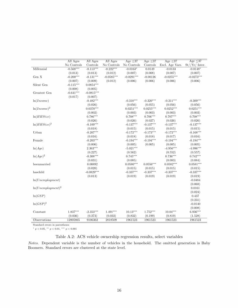
Millennial -0.568∗∗∗ -0.113∗∗∗ -0.222∗∗∗ -0.0163∗ 0.0149 -0.0133 -0.0148∗

(0.013) (0.013) (0.012) (0.007) (0.008) (0.007) (0.007)Gen X -0.200∗∗∗ -0.131∗∗∗ -0.0585∗∗∗ -0.0291∗∗∗ -0.00126 -0.0255∗∗∗ -0.0273∗∗∗

(0.007) (0.009) (0.012) (0.006) (0.006) (0.006) (0.006)Silent Gen -0.115∗∗∗ 0.0854∗∗∗

(0.008) (0.005)Greatest Gen -0.641∗∗∗ -0.0815∗∗∗

(0.017) (0.007)ln(Income) -0.482∗∗∗ -0.310∗∗∗ -0.320∗∗∗ -0.311∗∗∗ -0.309∗∗∗

(0.026) (0.056) (0.055) (0.056) (0.056)ln(Income)2 0.0370∗∗∗ 0.0251∗∗∗ 0.0255∗∗∗ 0.0252∗∗∗ 0.0251∗∗∗

(0.002) (0.003) (0.003) (0.003) (0.003)ln(HHSize) 0.786∗∗∗ 0.708∗∗∗ 0.706∗∗∗ 0.707∗∗∗ 0.708∗∗∗

(0.026) (0.026) (0.027) (0.026) (0.026)ln(HHSize)2 -0.109∗∗∗ -0.137∗∗∗ -0.137∗∗∗ -0.137∗∗∗ -0.137∗∗∗

(0.018) (0.015) (0.015) (0.015) (0.015)Urban -0.207∗∗∗ -0.172∗∗∗ -0.173∗∗∗ -0.172∗∗∗ -0.168∗∗∗

(0.016) (0.018) (0.018) (0.017) (0.016)Female -0.203∗∗∗ -0.194∗∗∗ -0.194∗∗∗ -0.194∗∗∗ -0.194∗∗∗

(0.006) (0.005) (0.005) (0.005) (0.005)ln(Age) 2.363∗∗∗ -5.021∗∗∗ -4.956∗∗∗ -4.996∗∗∗

(0.227) (0.562) (0.552) (0.557)ln(Age)2 -0.308∗∗∗ 0.745∗∗∗ 0.736∗∗∗ 0.742∗∗∗

(0.031) (0.085) (0.083) (0.084)beenmarried 0.00892 0.0580∗∗∗ 0.0556∗∗∗ 0.0582∗∗∗ 0.0581∗∗∗

(0.020) (0.015) (0.015) (0.015) (0.015)haschild -0.0829∗∗∗ -0.337∗∗∗ -0.337∗∗∗ -0.337∗∗∗ -0.337∗∗∗

(0.013) (0.019) (0.019) (0.019) (0.019)ln(Unemployment) -0.0484

(0.068)ln(Unemployment)2 0.0161

(0.024)ln(GSP ) 0.437

(0.231)ln(GSP )2 -0.0140

(0.008)Constant 1.837∗∗∗ -2.353∗∗∗ 1.491∗∗∗ 10.13∗∗∗ 1.752∗∗∗ 10.04∗∗∗ 6.936∗∗∗

(0.036) (0.373) (0.033) (0.832) (0.199) (0.819) (1.528)

Observations 12805865 9106362 2818509 1961523 1961523 1961523 1961523

Standard errors in parentheses∗ p < 0.05, ∗∗ p < 0.01, ∗∗∗ p < 0.001

Table A.2: ACS vehicle ownership regression results, select variables

Notes. Dependent variable is the number of vehicles in the household. The omitted generation is BabyBoomers. Standard errors are clustered at the state level.

16

All AgesNo Controls

All AgesControls

All AgesNo Controls

Age ≤37No Controls

Age ≤37Controls

Age ≤37Excl. Age Vars.

Age ≤37St//Yr/ Inter.

Millennial -1517.2∗∗∗ 172.1 -1824.0∗∗∗ 601.4∗ -83.08 650.4∗ 793.9∗

(190.963) (223.861) (270.837) (298.763) (305.312) (299.306) (307.445)Gen X 655.1∗∗∗ 743.5∗∗∗ 248.2 512.3 135.5 556.7 964.3∗∗

(133.272) (160.034) (237.919) (338.644) (361.403) (341.150) (294.411)Silent Gen -2997.3∗∗∗ -751.3∗∗∗

(151.957) (100.143)Greatest Gen -7178.6∗∗∗ -1775.4∗∗∗

(231.581) (228.072)ln(Income) 6291.8∗∗∗ 5574.9∗∗ 8118.6∗∗∗ 4991.0∗∗ 6030.3∗∗

(1126.146) (1808.421) (1889.778) (1750.194) (1856.303)ln(Income)2 -187.7∗∗ -171.4 -287.0∗∗ -143.7 -193.6∗

(53.691) (86.608) (90.609) (83.575) (88.980)High Income -118.2 -476.6 -650.7∗ -503.8 -199.9

(177.258) (285.305) (276.384) (309.264) (276.730)ln(HHSize) -521.1 -3934.4 -4842.1 -3986.7 -4348.2

(1185.778) (2435.818) (2451.835) (2396.301) (2427.920)ln(HHSize)2 -2.436 846.1 907.1 830.6 999.0

(422.347) (869.768) (857.368) (855.690) (866.515)Urban Cluster 833.5∗∗∗ 852.5∗∗ 837.5∗∗ 897.2∗∗ 1073.5∗∗∗

(131.378) (274.191) (280.870) (284.176) (255.854)Surrounded by Urban Areas 1352.7∗∗∗ 2196.8∗∗∗ 2107.6∗∗∗ 1210.2∗∗ 2712.1∗∗∗

(300.366) (417.615) (555.923) (426.546) (405.241)Not in Urban Area 3517.0∗∗∗ 4045.7∗∗∗ 4086.0∗∗∗ 4166.8∗∗∗ 4084.0∗∗∗

(167.556) (300.950) (303.264) (310.074) (287.342)High School 1288.9∗∗∗ 2059.2∗∗∗ 2757.7∗∗∗ 2002.2∗∗∗ 2018.6∗∗∗

(253.396) (515.557) (494.929) (530.311) (521.650)Some College 2020.6∗∗∗ 2722.5∗∗∗ 3615.9∗∗∗ 2634.7∗∗∗ 2670.1∗∗∗

(254.409) (459.610) (429.200) (478.839) (466.296)Bachelor’s 1098.1∗∗∗ 1174.6∗ 2562.1∗∗∗ 1067.3 1095.7

(252.909) (550.990) (494.120) (573.280) (563.063)Graduate Degree 215.2 163.7 1749.1∗∗∗ 71.39 52.69

(275.547) (511.826) (433.579) (522.669) (523.584)Female -5607.6∗∗∗ -4977.9∗∗∗ -5060.9∗∗∗ -4980.6∗∗∗ -4982.9∗∗∗

(184.607) (223.507) (230.671) (223.908) (226.405)ln(Age) 68107.6∗∗∗ 133512.1∗∗∗ 132900.9∗∗∗ 128292.1∗∗∗

(5043.360) (14965.700) (15365.617) (14893.825)ln(Age)2 -9310.8∗∗∗ -19329.3∗∗∗ -19240.6∗∗∗ -18510.6∗∗∗

(693.701) (2262.288) (2327.550) (2257.771)ln(GSP ) 9075.5∗

(3450.171)ln(GSP )2 -388.9∗∗

(130.303)ln(Unemployment) -3236.9

(5297.560)ln(Unemployment)2 876.1

(1372.319)Constant 13825.7∗∗∗ -157518.3∗∗∗ 14132.5∗∗∗ -255804.5∗∗∗ -41081.4∗∗∗ -253967.5∗∗∗ -301081.5∗∗∗

(258.843) (12969.411) (323.696) (26690.694) (9785.908) (27013.139) (30152.308)

Observations 484142 448058 102327 95654 95654 95654 95654

Standard errors in parentheses∗ p < 0.05, ∗∗ p < 0.01, ∗∗∗ p < 0.001

Table A.3: NHTS VMT regression results

Notes. Dependent variable is the number of miles driven by the respondent in the given year. The omittedgeneration is Baby Boomers. Standard errors are clustered at the state level.

17

Family Size Children Married Urban Income

Millennial 0.0191∗∗∗ 0.00718∗∗∗ -0.0180∗∗∗ 0.0372∗∗∗ 0.0215∗∗

(0.002) (0.002) (0.002) (0.002) (0.008)Gen X 0.0509∗∗∗ 0.0268∗∗∗ -0.00305∗ 0.0616∗∗∗ 0.0511∗∗∗

(0.001) (0.001) (0.001) (0.001) (0.005)2000 -0.129∗∗∗ -0.0815∗∗∗ -0.0651∗∗∗ -0.118∗∗∗ -0.0130∗∗

(0.001) (0.001) (0.001) (0.001) (0.004)2010 -0.133∗∗∗ -0.0863∗∗∗ -0.169∗∗∗ -0.111∗∗∗ -0.188∗∗∗

(0.002) (0.002) (0.002) (0.002) (0.006)2015 -0.142∗∗∗ -0.0987∗∗∗ -0.197∗∗∗ -0.0576∗∗∗ -0.172∗∗∗

(0.002) (0.002) (0.002) (0.002) (0.008)To Grade 4 0.149∗∗∗ 0.0665∗∗∗ 0.00909 0.00127 -0.0585∗

(0.015) (0.011) (0.011) (0.009) (0.024)Grade 5 to 8 0.168∗∗∗ 0.114∗∗∗ 0.0598∗∗∗ -0.0476∗∗∗ -0.00736

(0.009) (0.007) (0.006) (0.006) (0.016)Grade 9 0.121∗∗∗ 0.123∗∗∗ 0.0441∗∗∗ -0.0599∗∗∗ -0.00988

(0.009) (0.007) (0.007) (0.006) (0.016)Grade 10 0.0833∗∗∗ 0.112∗∗∗ 0.0312∗∗∗ -0.0712∗∗∗ 0.0333∗

(0.009) (0.006) (0.006) (0.006) (0.016)Grade 11 0.0990∗∗∗ 0.124∗∗∗ 0.0235∗∗∗ -0.0539∗∗∗ 0.0826∗∗∗

(0.008) (0.006) (0.006) (0.006) (0.016)Grade 12 0.0242∗∗ 0.0614∗∗∗ 0.0463∗∗∗ -0.0286∗∗∗ 0.436∗∗∗

(0.008) (0.006) (0.006) (0.005) (0.014)1 Year of College -0.0953∗∗∗ -0.0344∗∗∗ -0.00169 0.0458∗∗∗ 0.512∗∗∗

(0.008) (0.006) (0.006) (0.005) (0.014)2 Years of College -0.0902∗∗∗ -0.0442∗∗∗ 0.0304∗∗∗ 0.0291∗∗∗ 0.682∗∗∗

(0.008) (0.006) (0.006) (0.005) (0.015)4 Years of College -0.252∗∗∗ -0.200∗∗∗ -0.0646∗∗∗ 0.128∗∗∗ 0.903∗∗∗

(0.008) (0.006) (0.006) (0.005) (0.014)5+ Years of College -0.282∗∗∗ -0.228∗∗∗ -0.0457∗∗∗ 0.141∗∗∗ 1.063∗∗∗

(0.008) (0.006) (0.006) (0.005) (0.015)African American -0.0449∗∗∗ 0.0238∗∗∗ -0.191∗∗∗ 0.129∗∗∗ -0.377∗∗∗

(0.002) (0.001) (0.001) (0.001) (0.003)American Indian 0.0406∗∗∗ 0.0358∗∗∗ -0.0576∗∗∗ -0.107∗∗∗ -0.271∗∗∗

(0.006) (0.005) (0.005) (0.006) (0.011)Chinese -0.135∗∗∗ -0.0995∗∗∗ -0.0522∗∗∗ 0.0771∗∗∗ -0.267∗∗∗

(0.004) (0.003) (0.004) (0.003) (0.013)Japanese -0.171∗∗∗ -0.124∗∗∗ -0.110∗∗∗ 0.0567∗∗∗ -0.180∗∗∗

(0.008) (0.006) (0.007) (0.004) (0.018)Pacific Islander -0.0125∗∗∗ -0.0119∗∗∗ 0.0202∗∗∗ 0.0970∗∗∗ -0.110∗∗∗

(0.003) (0.003) (0.003) (0.002) (0.007)Other 0.146∗∗∗ 0.0947∗∗∗ 0.0116∗∗∗ 0.111∗∗∗ -0.133∗∗∗

(0.003) (0.002) (0.002) (0.002) (0.005)Two Major Races -0.0158∗∗∗ 0.00496 -0.0601∗∗∗ 0.0694∗∗∗ -0.194∗∗∗

(0.004) (0.004) (0.004) (0.004) (0.009)Three+ Major Races -0.0296∗ -0.00797 -0.0736∗∗∗ 0.0537∗∗∗ -0.177∗∗∗

(0.014) (0.012) (0.011) (0.012) (0.027)Female 0.0355∗∗∗ 0.117∗∗∗ -0.0719∗∗∗ 0.0370∗∗∗ -0.351∗∗∗

(0.001) (0.001) (0.001) (0.001) (0.002)ln(Age) 6.346∗∗∗ 2.038∗∗∗ 0.881∗∗∗ 0.866∗∗∗ 26.25∗∗∗

(0.098) (0.080) (0.081) (0.098) (0.315)ln(Age)2 -0.751∗∗∗ -0.153∗∗∗ 0.0346∗∗ -0.131∗∗∗ -3.632∗∗∗

(0.015) (0.012) (0.012) (0.015) (0.047)Constant -12.02∗∗∗ -4.667∗∗∗ -2.688∗∗∗ -0.566∗∗∗ -36.79∗∗∗

(0.158) (0.130) (0.131) (0.162) (0.528)

Observations 2818509 2818509 2818509 2134476 2518299

Standard errors in parentheses∗ p < 0.05, ∗∗ p < 0.01, ∗∗∗ p < 0.001

Table A.4: ACS demographics regression results, select variables

Notes. Dependent variable is listed in the column header. The omitted generation is Baby Boomers.Standard errors are clustered at the state level.

18

References

Abadie, A. and G. W. Imbens (2011): “Bias-Corrected Matching Estimators for Average Treat-

ment Effects,” Journal of Business & Economic Statistics, 29, 1–11.

Astone, N. M., S. Martin, and H. E. Peters (2016): “Millennial Childbearing and the

Recession,” https://www.urban.org/research/publication/millennial-childbearing-and-recession.

Buchholz, T. and V. Buchholz (2012): “The Go-Nowhere Generation,” The New York Times.

Dutzik, T., J. Inglis, and P. Baxandall (2014): “Millennials in Motion: Changing Travel

Habits of Young Americans and the Implications for Public Policy,” Working paper, U.S. PIRG,

Frontier Group.

Fry, R. (2017): “5 Facts about Millennial Households,” Working paper, Pew Research Center.

Kurz, C. J., G. Li, and D. J. Vine (2018): “Are Millennials Different?” .

Leard, B., J. Linn, and C. Munnings (2019): “Explaining the Evolution of Passenger Vehicle

Miles Traveled in the United States,” The Energy Journal, 40, 25–54.

Martin, S., N. M. Astone, and H. E. Peters (2016): “Fewer Mar-

riages, More Divergence: Marriage Projections for Millennials to Age 40,”

http://www.urban.org/research/publication/fewer-marriages-more-divergence-marriage-

projections-millennials-age-40.

Nielsen (2014): “Millennials Prefer Cities to Suburbs, Subways to Driveways,”

http://www.nielsen.com/us/en/insights/news/2014/millennials-prefer-cities-to-suburbs-

subways-to-driveways.html.

——— (2015): “Green Generation: Millennials Say Sustainability Is a Shopping

Priority,” http://www.nielsen.com/us/en/insights/news/2015/green-generation-millennials-say-

sustainability-is-a-shopping-priority.

Taylor, K. (2017): “Millennials Are Killing Chains like Buffalo Wild Wings and Applebee’s,”

http://www.businessinsider.com/millennials-endanger-casual-dining-restaurants-2017-5.

Thompson, D. and J. Weissman (September 2012 Issue): “The Cheapest Generation,” The

Atlantic.

19

MIT CEEPR Working Paper Series is published by the MIT Center for Energy and Environmental Policy Research from submissions by affiliated researchers.

Copyright © 2019Massachusetts Institute of Technology

MIT Center for Energy and Environmental Policy Research 77 Massachusetts Avenue, E19-411Cambridge, MA 02139 USA

Website: ceepr.mit.edu

For inquiries and/or for permission to reproduce material in this working paper, please contact:

Email ceepr@mit.eduPhone (617) 253-3551Fax (617) 253-9845

Since 1977, the Center for Energy and Environmental Policy Research (CEEPR) has been a focal point for research on energy and environmental policy at MIT. CEEPR promotes rigorous, objective research for improved decision making in government and the private sector, and secures the relevance of its work through close cooperation with industry partners from around the globe. Drawing on the unparalleled resources available at MIT, affiliated faculty and research staff as well as international research associates contribute to the empirical study of a wide range of policy issues related to energy supply, energy demand, and the environment. An important dissemination channel for these research efforts is the MIT CEEPR Working Paper series. CEEPR releases Working Papers written by researchers from MIT and other academic institutions in order to enable timely consideration and reaction to energy and environmental policy research, but does not conduct a selection process or peer review prior to posting. CEEPR’s posting of a Working Paper, therefore, does not constitute an endorsement of the accuracy or merit of the Working Paper. If you have questions about a particular Working Paper, please contact the authors or their home institutions.