1

Generational Differences in Mexican-American’s Earnings:

Comparing the Second and Third Generation1

Yukio Kawano

Daito-Bunka University

Tokyo, Japan

Katharine M. Donato

Rice University

Charles Tolbert

Baylor University

1 Part of this research was funded by the Center of Social Stratification and Inequality (CSSI), the Center of Excellence (COE) Program at Tohoku University, Japan.

2

Abstract

Generational economic progress of Mexican Americans is stagnant in terms of earnings.

Using the Current Population Survey data from 1994 to 2003, we test if earnings of the

third generation Mexicans are different from that of the second generation. We classify

two types of the second generation: one who has one Mexican-born parent (SG-1) and

another who has two (SG-2), and analyze male and female workers separately. Among

females, we do not find significant difference between the two generations after

controlling for human capital, urban residence, and industry in which they work.

Among males, SG-2 makes just as much earnings as the third generation does. These

results suggest that Mexican American’s earnings in general do not change by

generation. Exceptionally, male children with mixed-nativity parents (SG-1) earn

significantly greater than the third. We assume such parents are better equipped with

resources to support their male children’s adaptation.

3

Introduction

Hispanic population in the United States had increased rapidly by more than 50 percent

from 22.4 million in 1990 to 35.3 million in 2000, of which the single largest group is

Mexican – 58% of total Hispanic in 2000 census (Census Bureau 2001). The number

represents not only the new adult immigrants but also a number of their children born

and grow up in the United States. As those children start working in the U.S. labor

market, their economic outcomes become increasingly important because of their size

and slow socioeconomic adaptation. For many Mexican parents who have low

education and low-wage jobs, it is difficult to provide their children with enough

resources and opportunities to succeed at school and in the labor market. Despite the

prediction of the classic linear assimilation theory in which immigrant families

overcome their disadvantages over generations through acculturation and economic

adaptation, the earnings growth of the Mexican Americans seem stagnant or even

declining as they move on to later generations.

In order to approach the problem of generational economic progress of Mexican

Americans, we study earnings of their second and third generations. Mexican

Americans are distinguished into three different generation groups: the second

generation is those who have one parent born in Mexico and two parents born there; the

third generation is those whose both parents were born in the United States. (We

elaborate on these definitions in the following sections.) We mainly focus on the

comparison between second and third generations because the improvement from first

to second generation is too obvious. Owing to better accumulation of human capital

such as English and education, second and later generations always achieve better than

4

the first generation. The real problem for the Mexican American is the trajectory after

the second generation, and whether the path is upward, downward or stagnant.

This topic has not been well researched because of two practical reasons: data

limitation and relative youth of Mexican Americans. First, it is difficult to identify

generation in available public data because information about parents’ immigration

status is limited. Secondly, a number of second-generation Mexicans were still in

schools and haven’t started working. Thus researchers were unable to find their large-

enough sample in the labor market. Only recently, they grew up to enter the labor

market and enable researchers to find the reasonable number of samples.

Background

Studies on intergenerational progress of immigrants and their children can be

summarized in three perspectives: linear, curvilinear, and segmented assimilation. First,

based on the experience of European immigrants, the linear assimilation perspective

expects immigrants and their descendants to eventually assimilate into the mainstream

of the host society (native whites) after about three generations. However, research on

non-European immigrants shows that the gap between minority and mainstream

Americans are not diminishing, but sometimes even increasing. Such reality inspired

many alternative views. One of which suggests that these ethnic minorities will take not

“linear” but “bumpy” road to assimilation (Gans 1992). Using historical census data,

Smith (2003) found that Mexican American’s income is relatively growing but the

progress from second to third generation had decelerated in recent years.

Secondly, the “curvilinear assimilation” perspective, also called immigrant

optimism, expects better achievement of the second generation than the later

5

generations as a result of foreign parentage. When plotting achievements of first,

second and third generation in order, the second generation’s overachievement and the

third generation’s underachievement make a convex curve. This view assumes that

high motivation and work discipline are transmitted from the first generation parents to

their children. The second generation combines the high motivation and high

educational attainment to achieve not only better than the first generation, but also better

than the third generation. The third generation cannot exceed the second because all the

native-born are given same educational opportunities and the first generation’s

motivation diminishes after the second generation.

The third view, which we call stagnation or “segmented assimilation”

perspective, argues that descendants of non-European immigrants will not completely

converge with mainstream population, but assimilate into their own “segment” in terms

of socio-economic status (Portes and Rumbaut 2001). In this view, ethnic minorities do

not achieve parity with the mainstream American but lose upward or downward

momentum – getting stuck there. This perspective, as we will show in this report,

explains most appropriately the Mexican-American workers’ situation in which being

second or third generation does not make much difference.

The second view, the curvilinear theory, is extended from earlier research on

second-generation children at school. Studies on children’s educational achievements

and foreign parentage started much earlier and continuing (Kao and Tienda 1995; Kao

and Thompson 2003; Pong 2003). They found that native-born children of at least one

foreign-born parent not only achieve better than their foreign-born classmates, but also

outperform their third generation classmates. Researchers explain that immigrants’

emotional and disciplinary devotion to their children’s education, their “optimism”

6

about their future in the U.S., affect positively on the children’s aspiration and academic

achievement. However, the third and later generations do not achieve as much as the

second because their parents are native-born and they do not have the devotion to

education that immigrants’ family does. Empirically, this hypothesis found support

from Asian children and much less from Mexican/Latinos and none from black and

white children (Kao and Tienda 1995).

If this second-generation overachievement is true, and the generational

difference in school achievements affects economic outcomes in the labor market,

generational earnings differentials should also decline in and after the third generation.

Earlier empirical studies on this issue used 1970 census because it provided birthplace

of respondent’s parents. (Parents’ birthplace question had been replaced by ancestry

question after this census). Chiswick (1977) reported that U.S.-born “white” children of

at least one foreign-born parent have higher earning than those having two native

parents. Carliner (1980) tested other ethnic groups as well and found higher earnings of

second-generation males than the third generation.

However, these research had reservations as to applicability of the second-

generation advantage to all ethnic groups. In education, Kao and Tienda (1995) showed

that foreign parentage is more beneficial to Asians than to Hispanics. Chiswick (1997)

also pointed out significant disadvantage, not advantage, of having Mexican-born

parents. Carliner (1980) also noted that, among five ethnic groups he tested, only

Filipino Americans showed statistically significant decline from the second to third

generation.

Ethnic diversity in the United States increased after 1970s. To study

generational difference by ethnicity, researchers need to use data sources other than

7

census. Using CPS (Current Population Survey) data, Grogger and Trejo (2002) found

no significant difference between second and third-generation Mexican Americans in

terms of earnings. But Livingston and Kahn (2002), using LNPS (Latino National

Political Survey) and PSID (Panel Study of Income Dynamics), observed a curvilinear

pattern in which second-generation Mexican Americans earn more than the third

generation. The disagreement between these two studies is mainly due to interpretation

of statistics in the latter. Based on the sample of 56,000 Mexicans, of which about half

is the first and the rest is the second or third generation, Grogger and Trejo found the

second and third generation received statistically equivalent earnings. Livingston and

Kahn, on the other hand, identified only 553 Mexicans for three generations and found

no significant difference between the second and third generations. However, they

concluded that the curvilinear pattern does exist among Mexicans because the

regression coefficients for the third generation relative to the second was consistently

negative across models. Such interpretation is questionable as long as the chance of the

coefficient to be non-zero is insignificant. Consistency or inconsistency of coefficient’s

direction can be easily manipulated by model specification. If the lack of statistical

significance is due to the small sample size, they should have re-tested it using larger

samples.

Before embarking on our empirical research, three issues should be addressed

(see Grogger and Trejo 2003: pp. 6-8). First, generational progress and changes in the

quality of entry cohort can be confounded to the extent that different cohort quality is

transmitted to next generations, causing over- or under-estimation of intergenerational

changes (Borjas 1993; 1995). Suppose that earlier entry cohort of immigrants have

much better skills than current entry cohort, then the children of the earlier cohort (old

8

second generation) will be more qualified than the children of current immigrants (new

second generation) would ever become; but when the new second generation are still

small children, we have to use the old second generation to approximate what the new

second generation would make when they grow up, which causes overestimation. Since

we do not match parents and children in the dataset, children of current first and second

generation may have different characteristics than the current second and third

generation, respectively. As for Mexican, since their cohort quality is improving (Smith

2003), third generation earning will only be underestimated.

Secondly, if there is significant difference between Mexican migrants who stay

in the U.S. and who leave the country, then estimates based on the remaining population

may be biased. If this is the case, longer stay in the U.S. means not only they have

greater experience, but also they survived using their better quality. There are many

attempts to assess this issue but arguments in both sides – biased or nonbiased

selections – are at best inconclusive.

Thirdly, those who keep identifying themselves as Mexican after three or more

generations can be doing so because they think that they belong to a disadvantaged

minority group who failed in adaptation. Because parents’ race and ethnicity are not

available in most data, we cannot identify Mexicans who no longer associate themselves

with the Mexican label. To access if exclusion of such individuals causes any bias in

our estimation, we conducted a preliminary analysis on the second generation with self-

identified Mexicans and those without self-identity (see Data and Method section).

9

This Research

In this paper, we focus on the hourly earning differentials of male and female Mexican

workers in the United States in terms of foreign-born parentage or, in other words,

second-third generation comparison. Many research have compared three generations,

but we decide to focus only on the second and third generations because the

improvement from the first to second generation is incontestable (though we show some

descriptive statistics on the foreign-born Mexicans).

In addition, in terms of transmission of positive resource, i.e. motivation, from

foreign parent, the question is how advantageous it is to have, or not to have, parent(s)

born in Mexico. In considering the second-generation advantage, we pay attention to

the fact that, when a second-generation child has at least one Mexican-born parent, she

or he has one parent from non-Mexican or native-born background. If a typical second-

generation Mexican has parents who are both Mexican born, those having only one

Mexican-born parent should fit in a different category. A recent report showed that

exogamous Mexican couples (Mexicans married non-Mexicans) are substantially better

educated than endogamous Mexican couples (Duncan and Trejo 2004)2.

We have not seen any research reporting positive effect of Mexican parentage on

the educational achievement, or attainment, of second-generation Mexican children.

Being Mexican at school implies disadvantage in terms of academic performance as

well as aspiration (Portes and Hao 2004; Pong 2003). Low accumulation of human

capital leads to low socio-economic status, and often to the cycle of poverty which

immobilizes Mexican stratum in American society (Portes and Rumbaut 2001). With

2 In the following, we do not replicate the Duncan and Trejo’s distinction but separate foreign-born parents from mixed-nativity parents. Due to data limitation we do not know ethnic identities of one native parent, but as Duncan and Trejo reported in the same study, the parents are likely to be both Mexican with mixed nativity when their children identify themselves as Mexican.

10

this reasoning we do not expect positive effect of Mexican parentage on the earnings of

the second generation either, and thus support the segmented assimilation theory in

explaining the earning difference of Mexican-American workers.

We proceed our analysis in two steps. First, after reviewing some descriptive

facts, i.e. wage gaps, demographic and human capital distribution, etc., we examine

industry and occupation structure of Mexican workers because we expect that, in

segmented assimilation, they are trapped in their low status jobs regardless of their

generations. To clarify the position of second- and third-generation Mexicans, we also

bring in first generation Mexicans as well as native non-Hispanic whites and blacks.

The main question in this step is whether second- and third-generation Mexicans are

different in terms of industry and occupation composition. We analyze males and

females separately because their occupational as well as career patterns are very

distinctive.

Secondly, we examine the “third generation decline” or “second generation

overachievement” in Mexican American workers by directly comparing second and

third generation in multivariate regression. Using hourly earnings of Mexican workers

as a dependent variable, we focus on the effect of having or not having at least one

Mexican-born parent, controlling for other demographic, geographic, and human capital

factors. The purpose of this operation is to see if significant second-generation

advantage over the third generation exists.

Data and Method

We use Outgoing Rotation Group (ORG) sample from Current Population Survey

(CPS) Basic Monthly Files collected from 1994 to 2003 (Census Bureau 2002).

11

Monthly samples consist of eight rotation groups. They are called rotation groups

because one rotation group enters the survey every month to replace another group

which already had four interviews in the previous four months. After the fourth month,

they leave the sample and come back to the survey after eight months to complete four-

month interviews again, and then go out of the sample for the last time. The groups at

their fourth and eighth interview months are called Outgoing Rotation Group (ORG).

We use ORG because information on earnings is available only in this group. Of the

fourth and eighth month groups, we keep only persons at the fourth month in order to

avoid the problem of non-independent sample when data is pooled over multiple years.3

CPS samples about 50,000 civilian, non-institutionalized, households every month,

which enable us to obtain a large number of minority observations. However, it lacks

language-related variables such as English proficiency. In addition, there are coding

problems in the “place of birth” item in 1994-96, but it affects mainly those who were

born in Asian countries and not Mexican (Census Bureau 1998). Another coding

problem occurred in 1995 led to missing metropolitan status.

In order to focus on labor force population, we limit our sample to male and

female wage earners (excluding self-employed workers) who are 25 to 59 years old,

work more than 10 hours per week, and earn $1 - $500 per hour. This definition drops

all students and most of non-full time workers. The final sample is mostly comparable

with that in Grogger and Trejo (2003). We define the three generations of Mexicans

and Mexican Americans4 as follows: all of them identify themselves as Mexican

(Mexican American, Chicano, or Mexican); first-generation Mexicans are those who

3 Approximately a quarter of households and individuals overlap from month to month, and a half overlap from year to year. 4 Foreign-born persons inevitably include those who have not naturalized and therefore not American. So we call the first generation just Mexican although many of them are American citizens for simplicity.

12

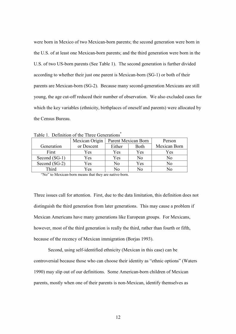
were born in Mexico of two Mexican-born parents; the second generation were born in

the U.S. of at least one Mexican-born parents; and the third generation were born in the

U.S. of two US-born parents (See Table 1). The second generation is further divided

according to whether their just one parent is Mexican-born (SG-1) or both of their

parents are Mexican-born (SG-2). Because many second-generation Mexicans are still

young, the age cut-off reduced their number of observation. We also excluded cases for

which the key variables (ethnicity, birthplaces of oneself and parents) were allocated by

the Census Bureau.

Table 1. Definition of the Three Generations*

Parent Mexican Born Generation

Mexican Origin or Descent Either Both

Person Mexican Born

First Yes Yes Yes Yes

Second (SG-1) Yes Yes No No

Second (SG-2) Yes No Yes No

Third Yes No No No “No” to Mexican-born means that they are native-born.

Three issues call for attention. First, due to the data limitation, this definition does not

distinguish the third generation from later generations. This may cause a problem if

Mexican Americans have many generations like European groups. For Mexicans,

however, most of the third generation is really the third, rather than fourth or fifth,

because of the recency of Mexican immigration (Borjas 1993).

Second, using self-identified ethnicity (Mexican in this case) can be

controversial because those who can choose their identity as “ethnic options” (Waters

1990) may slip out of our definitions. Some American-born children of Mexican

parents, mostly when one of their parents is non-Mexican, identify themselves as

13

“other” ethnicity. Their ambiguity forced us to exclude them from our sample.5 We

realize that the identity of multi-ethnic or mixed-nationality family is a very important

problem. However, so far as this research is concerned, we need to balance distinctions

of third generation and second generation: because self-identity is the only way to

define the third generation Mexican Americans, we limit the second generation to self-

identified Mexicans in order to maintain their comparability.

The third issue is the definition of the second generation Mexicans who have

just one Mexican-born parent. Having only one Mexican-born parent means that she

may have one non-Mexican-born (native) parent as well.6 Past research failed to

consider that native-born mothers and fathers may also have significant, perhaps

positive, effect on their children’s labor market performance because of their command

in English, education, knowledge about U.S. labor market, social connections, etc. It is

therefore necessary to distinguish the different types of foreign parentage.

Description

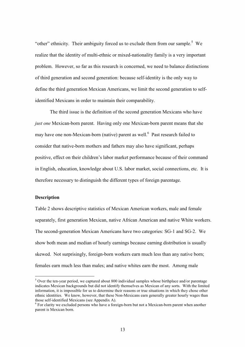
Table 2 shows descriptive statistics of Mexican American workers, male and female

separately, first generation Mexican, native African American and native White workers.

The second-generation Mexican Americans have two categories: SG-1 and SG-2. We

show both mean and median of hourly earnings because earning distribution is usually

skewed. Not surprisingly, foreign-born workers earn much less than any native born;

females earn much less than males; and native whites earn the most. Among male

5 Over the ten-year period, we captured about 800 individual samples whose birthplace and/or parentage indicates Mexican backgrounds but did not identify themselves as Mexican of any sorts. With the limited information, it is impossible for us to determine their reasons or true situations in which they chose other ethnic identities. We know, however, that these Non-Mexicans earn generally greater hourly wages than those self-identified Mexicans (see Appendix A). 6 For clarity we excluded persons who have a foreign-born but not a Mexican-born parent when another parent is Mexican born.

14

Table 2 M

ean Characteristics of Mexican Generation Groups, Black and W

hite Natives 1994-2002(3)

MALE

FEMALE

Mexican

Mexican

Mexican

Mexican Native NH Native NH Mexican

Mexican

Mexican

Mexican Native NH N

ative NH

1st Gen

2nd Gen

(SG-1)

2nd Gen

(SG-2)

3rd Gen

Black

White

1st Gen

2nd Gen

(SG-1)

2nd Gen

(SG-2)

3rd Gen

Black

White

Hourly Earning ($)**

9.77

14.90

13.39

13.96

13.02

18.02

7.98

11.87

11.45

11.41

11.69

13.84

(.052)

(.263)

(.224)

(.111)

(.048)

(.022)

(.061)

(.237)

(.202)

(.092)

(.039)

(.018)

(Median)

8.27

12.73

11.58

12.04

11.15

15.48

6.80

10.08

9.60

9.71

9.78

11.65

Age (years)

36.53

39.46

35.85

38.36

39.40

40.49

37.84

39.52

36.12

38.64

39.61

40.84

(.079)

(.299)

(.271)

(.121)

(.059)

(.019)

(.118)

(.307)

(.291)

(.123)

(.051)

(.020)

Married

0.67

0.70

0.61

0.65

0.53

0.70

0.63

0.59

0.55

0.57

0.37

0.65

(.004)

(.014)

(.014)

(.006)

(.003)

(.001)

(.007)

(.016)

(.015)

(.007)

(.003)

(.001)

High School

0.34

0.83

0.76

0.80

0.89

0.93

0.41

0.84

0.82

0.83

0.91

0.95

(.004)

(.012)

(.012)

(.005)

(.002)

(.001)

(.007)

(.012)

(.012)

(.005)

(.002)

(.000)

Part Tim

e 0.04

0.04

0.05

0.04

0.05

0.03

0.18

0.15

0.14

0.15

0.11

0.18

(.002)

(.006)

(.006)

(.003)

(.001)

(.000)

(.005)

(.012)

(.010)

(.005)

(.002)

(.001)

Central city

0.42

0.29

0.34

0.32

0.42

0.16

0.41

0.33

0.35

0.34

0.44

0.17

(.005)

(.014)

(.014)

(.006)

(.003)

(.001)

(.007)

(.015)

(.014)

(.007)

(.003)

(.001)

Occupation 7

High Skill

0.05

0.21

0.17

0.19

0.19

0.33

0.08

0.28

0.26

0.26

0.27

0.40

(.002)

(.013)

(.011)

(.005)

(.003)

(.001)

(.004)

(.015)

(.013)

(.006)

(.003)

(.001)

M

iddle Skill

0.37

0.45

0.46

0.47

0.39

0.44

0.31

0.51

0.52

0.52

0.44

0.45

(.004)

(.015)

(.014)

(.007)

(.003)

(.001)

(.006)

(.016)

(.015)

(.007)

(.003)

(.001)

Low Skill

0.59

0.34

0.38

0.34

0.42

0.23

0.61

0.21

0.22

0.21

0.29

0.16

(.005)

(.015)

(.014)

(.006)

(.003)

(.001)

37.84

39.52

36.12

38.64

39.61

40.84

n

11,522

1,047

1,200

5,434

23,220

226,837

5,443

941

1,122

5,180

31,230

213,220

Source: CPS 1994-2003. Standard errors are in parentheses * Different parentage. See text. ** Adjusted to 1998 dollars using Consumer Price Index. W

eighted.

7 See footnote 9 for categorization of occupations.

15

workers, all native Mexican workers earn more than native black workers, while the two

groups of native-Mexican females earn somewhat less than native black females. For

both males and females, having one native parent seems to give SG-1 workers a slight

advantage over SG-2 as well as over the third generation. However, further analysis is

needed to determine how significant the advantage is.

Mexican SG-1 workers, male or female, are more likely to be older, married,

and have high school or higher education than other Mexican American workers; they

are less likely to live in central city; and female SG-1 workers are more likely to work

part-time. In the occupational composition, SG-1 is somewhat more concentrated in

high-skill jobs than other two Mexican-American groups.8 As Table 2 shows, 21% of

SG-1 males are in high-skill occupations compare to 17% and 19% of SG-2 and the

third generation respectively; also 28% of SG-1 females vs. 26% of later generations.

The three native-Mexican groups, male and female, have the largest stock in the

Middle-Skill level and somewhat less in the low level, indicating that their occupational

compositions are somewhere between blacks and whites: blacks have its largest member

in the lowest level; whites have a large middle layer but the size of the high-skill layer is

greater than the lower one. We elaborate on the difference among native Mexicans in

terms of industry and occupation in the next section.

Industry and Occupation

8 We made this occupational-skill category based on the average earnings of Mexican workers in both sexes. (1) High-skill occupations include: executive, administrative, and managerial, professional, and specialty occupations. (2) Middle skilled occupations are: technicians and related support, sales, administrative support including clerical jobs, protective and other services, precision production, craft and repair occupations. (3) Low skill occupations are private household, machine operators, assemblers and inspectors, transportation and material moving occupations, handlers, equipment cleaners, helpers, laborers, farming, forestry and fishing occupations

16

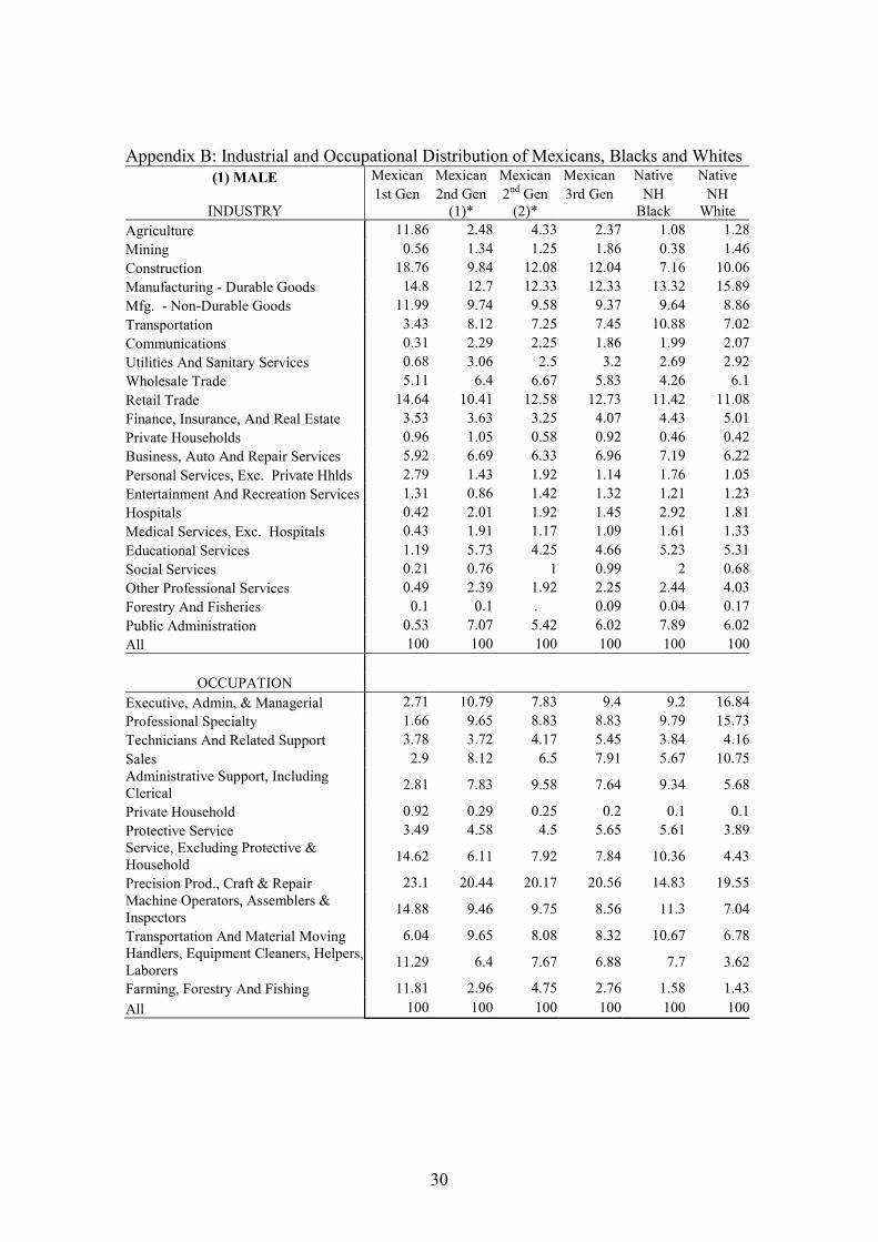
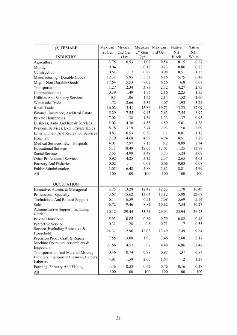
Table 3 indicates industrial compositions of the three-generation Mexicans as well as

that of native non-Hispanic blacks and whites. The industry classification was reduced

from twenty-two to eight categories to secure cell counts. Detailed table with the

twenty-two industries and twelve occupations are available in Appendix B.

First generation Mexicans show very specific job profile implying their

immigration history, network recruiting, and lack of human capital. Large part of them

work in low-paid, physical jobs in agriculture, construction, manufacturing, and

personal services (such as maids in case of women). Since these jobs are often

associated with poverty and undesirable working conditions, their children born in the

U.S. need to strive to break out of this job structure to find well-paid and comfortable

jobs. We find great gender differences in the industry composition. More males work

in manual jobs and more females work in trade (wholesale and retail) and service

industries.

Second- and third-generation Mexicans have clearly advanced from the first

generation in terms of industry composition. For example, while nearly one-third of the

first-generation males are employed in agriculture and construction, only 14 to 18

percent of native-born Mexicans work in the same industries. Also, native-born

Mexicans are finding jobs in industries in which not so many first-generation Mexicans

but native blacks and whites are working, e.g. transportation and communication (class

4) and service (class 7) industries.

17

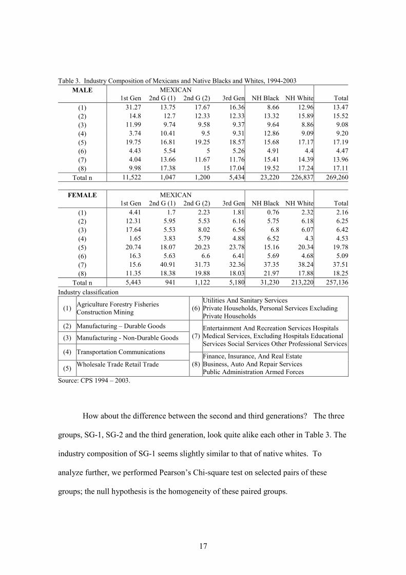
Table 3. Industry Composition of Mexicans and Native Blacks and Whites, 1994-2003

MALE MEXICAN

1st Gen 2nd G (1) 2nd G (2) 3rd Gen NH Black NH White Total

(1) 31.27 13.75 17.67 16.36 8.66 12.96 13.47

(2) 14.8 12.7 12.33 12.33 13.32 15.89 15.52

(3) 11.99 9.74 9.58 9.37 9.64 8.86 9.08

(4) 3.74 10.41 9.5 9.31 12.86 9.09 9.20

(5) 19.75 16.81 19.25 18.57 15.68 17.17 17.19

(6) 4.43 5.54 5 5.26 4.91 4.4 4.47

(7) 4.04 13.66 11.67 11.76 15.41 14.39 13.96

(8) 9.98 17.38 15 17.04 19.52 17.24 17.11

Total n 11,522 1,047 1,200 5,434 23,220 226,837 269,260

FEMALE MEXICAN

1st Gen 2nd G (1) 2nd G (2) 3rd Gen NH Black NH White Total

(1) 4.41 1.7 2.23 1.81 0.76 2.32 2.16

(2) 12.31 5.95 5.53 6.16 5.75 6.18 6.25

(3) 17.64 5.53 8.02 6.56 6.8 6.07 6.42

(4) 1.65 3.83 5.79 4.88 6.52 4.3 4.53

(5) 20.74 18.07 20.23 23.78 15.16 20.34 19.78

(6) 16.3 5.63 6.6 6.41 5.69 4.68 5.09

(7) 15.6 40.91 31.73 32.36 37.35 38.24 37.51

(8) 11.35 18.38 19.88 18.03 21.97 17.88 18.25

Total n 5,443 941 1,122 5,180 31,230 213,220 257,136

Industry classification

(1) Agriculture Forestry Fisheries Construction Mining

(6) Utilities And Sanitary Services Private Households, Personal Services Excluding Private Households

(2) Manufacturing – Durable Goods

(3) Manufacturing - Non-Durable Goods (7) Entertainment And Recreation Services Hospitals Medical Services, Excluding Hospitals Educational Services Social Services Other Professional Services

(4) Transportation Communications

(5) Wholesale Trade Retail Trade

(8) Finance, Insurance, And Real Estate Business, Auto And Repair Services Public Administration Armed Forces

Source: CPS 1994 – 2003.

How about the difference between the second and third generations? The three

groups, SG-1, SG-2 and the third generation, look quite alike each other in Table 3. The

industry composition of SG-1 seems slightly similar to that of native whites. To

analyze further, we performed Pearson’s Chi-square test on selected pairs of these

groups; the null hypothesis is the homogeneity of these paired groups.

18

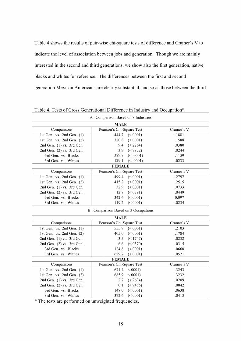
Table 4 shows the results of pair-wise chi-square tests of difference and Cramer’s V to

indicate the level of association between jobs and generation. Though we are mainly

interested in the second and third generations, we show also the first generation, native

blacks and whites for reference. The differences between the first and second

generation Mexican Americans are clearly substantial, and so as those between the third

Table 4. Tests of Cross Generational Difference in Industry and Occupation*

A. Comparison Based on 8 Industries

MALE

Comparisons Pearson’s Chi-Square Test Cramer’s V

1st Gen. vs. 2nd Gen. (1) 444.7 (<.0001) .1881

1st Gen. vs. 2nd Gen. (2) 320.8 (<.0001) .1588

2nd Gen. (1) vs. 3rd Gen. 9.4 (<.2264) .0380

2nd Gen. (2) vs. 3rd Gen. 3.9 (<.7872) .0244

3rd Gen. vs. Blacks 389.7 (< .0001) .1159

3rd Gen. vs. Whites 129.1 (< .0001) .0233

FEMALE

Comparisons Pearson’s Chi-Square Test Cramer’s V

1st Gen. vs. 2nd Gen. (1) 499.4 (<.0001) .2797

1st Gen. vs. 2nd Gen. (2) 415.2 (<.0001) .2515

2nd Gen. (1) vs. 3rd Gen. 32.9 (<.0001) .0733

2nd Gen. (2) vs. 3rd Gen. 12.7 (<.0791) .0449

3rd Gen. vs. Blacks 342.6 (<.0001) 0.097

3rd Gen. vs. Whites 119.2 (<.0001) .0234

B. Comparison Based on 3 Occupations

MALE

Comparisons Pearson’s Chi-Square Test Cramer’s V

1st Gen. vs. 2nd Gen. (1) 555.9 (<.0001) .2103

1st Gen. vs. 2nd Gen. (2) 405.0 (<.0001) .1784

2nd Gen. (1) vs. 3rd Gen. 3.5 (<.1747) .0232

2nd Gen. (2) vs. 3rd Gen. 6.6 (<.0370) .0315

3rd Gen. vs. Blacks 124.8 (<.0001) .0660

3rd Gen. vs. Whites 629.7 (<.0001) .0521

FEMALE

Comparisons Pearson’s Chi-Square Test Cramer’s V

1st Gen. vs. 2nd Gen. (1) 671.4 <.0001) .3243

1st Gen. vs. 2nd Gen. (2) 685.9 <.0001) .3232

2nd Gen. (1) vs. 3rd Gen. 2.7 (<.2634) .0209

2nd Gen. (2) vs. 3rd Gen. 0.1 (<.9456) .0042

3rd Gen. vs. Blacks 148.0 (<.0001) .0638

3rd Gen. vs. Whites 372.6 (<.0001) .0413

* The tests are performed on unweighted frequencies.

19

generation and other native-born Americans (blacks and whites). However, we do not

find much change between second and third generations: substantial differences are

found only between SG-1 and the third generation in female industries, and SG-2 and

the third generation in male occupations.

The strong association between their job and generational grouping indicates

their advancement in generational status “causes” different job compositions through

economic adaptation. For example, compared to the first generation females, much less

second-generation females work in agriculture, manufacture, and personal service

industries, and much more work in professional services (7) and more advanced

business service industries (8). Such transformation in job composition reflects on the

large Cramer’s Vs in female occupational and industrial compositions. However, such

dramatic job transitions do not happen after the second generation, as it is indicated in

the comparison between the second and third generations. Because the second- and

third-generation Mexicans are almost homogenous in terms of industry-occupation

composition, we conclude here that job transitions do not occur between the second and

third generations. In other words, the dramatic job transition of Mexican Americans

ceases at the second generation, and gain stable position in the labor market. As implied

in the comparison between the third and other native-born Americans, the industrial

composition of Mexican Americans is similar to that of whites, but their occupational

pattern is similar to that of blacks. It implies that generally Mexican Americans work

low-wage occupations in the white industries and it is hard for them to move out of this

structure.

20

Analyses

Our analyses thus far do not find a significant difference between second and third

generations, and indicate a stagnant path of Mexican-Americans over generations. A

unique finding is the distinction between two second-generation groups: SG-1 and SG-2.

Their difference in industry and occupation structure seems not quite great but

important, because the SG-1’s advantage may be just enough to explain the difference

in earnings between second and third generations. In previous research of the

curvilinear perspective, the key finding was the advantage of the second generation, but

such advantage may be easily explained away by the fact these studies had been mixing

up SG-1 and SG-2. So far as we have observed, SG-1 is on average slightly older,

better educated, having more high-skill jobs (Table 2), less likely to work in agriculture

and more likely to be professional worker than SG-2. It is therefore possible that, if we

take the difference of these two groups into account in multivariate models, we have

much clearer picture of generational advancement of Mexican-American workers.

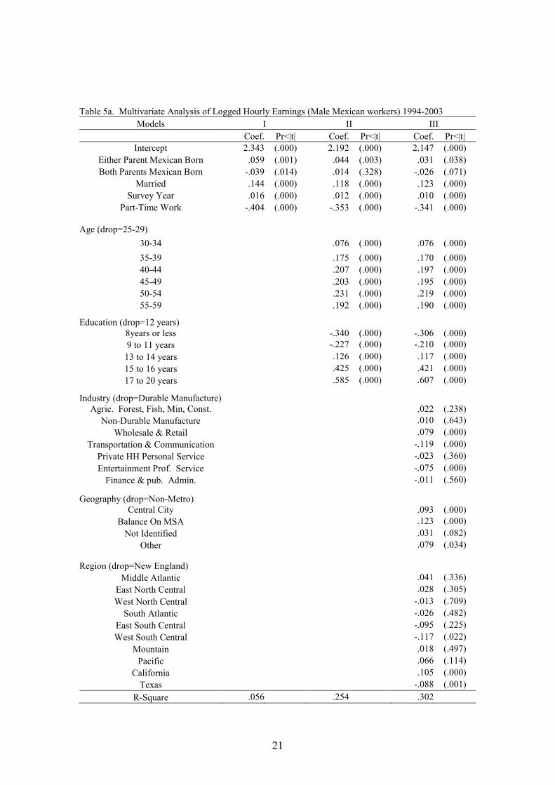
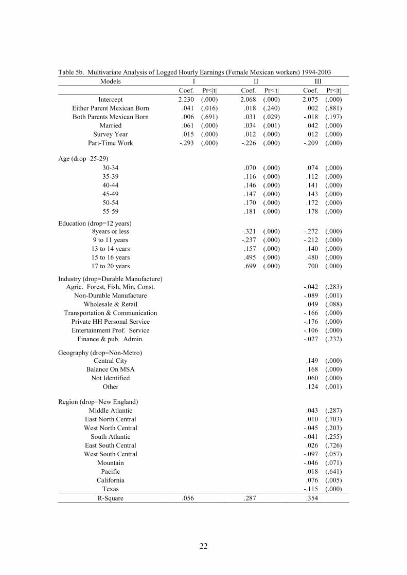
Table 5a and 5b are the results of our multivariate analyses on logged hourly

earnings of Mexican-American workers. We display three nested models for males and

females in Table 5a and 5b respectively. Model I includes basic controls in addition to

dummy variables setting to indicate “Either Parent Mexican Born” (SG-1) and “Both

Parents Mexican born” (SG-2). These two dummies indicate two types of the second

generation. The third generation is a reference group.

21

Table 5a. Multivariate Analysis of Logged Hourly Earnings (Male Mexican workers) 1994-2003

Models I II III

Coef. Pr<|t| Coef. Pr<|t| Coef. Pr<|t|

Intercept 2.343 (.000) 2.192 (.000) 2.147 (.000)

Either Parent Mexican Born .059 (.001) .044 (.003) .031 (.038)

Both Parents Mexican Born -.039 (.014) .014 (.328) -.026 (.071)

Married .144 (.000) .118 (.000) .123 (.000)

Survey Year .016 (.000) .012 (.000) .010 (.000)

Part-Time Work -.404 (.000) -.353 (.000) -.341 (.000)

Age (drop=25-29)

30-34 .076 (.000) .076 (.000)

35-39 .175 (.000) .170 (.000)

40-44 .207 (.000) .197 (.000)

45-49 .203 (.000) .195 (.000)

50-54 .231 (.000) .219 (.000)

55-59 .192 (.000) .190 (.000)

Education (drop=12 years)

8years or less -.340 (.000) -.306 (.000)

9 to 11 years -.227 (.000) -.210 (.000)

13 to 14 years .126 (.000) .117 (.000)

15 to 16 years .425 (.000) .421 (.000)

17 to 20 years .585 (.000) .607 (.000)

Industry (drop=Durable Manufacture)

Agric. Forest, Fish, Min, Const. .022 (.238)

Non-Durable Manufacture .010 (.643)

Wholesale & Retail .079 (.000)

Transportation & Communication -.119 (.000)

Private HH Personal Service -.023 (.360)

Entertainment Prof. Service -.075 (.000)

Finance & pub. Admin. -.011 (.560)

Geography (drop=Non-Metro)

Central City .093 (.000)

Balance On MSA .123 (.000)

Not Identified .031 (.082)

Other .079 (.034)

Region (drop=New England)

Middle Atlantic .041 (.336)

East North Central .028 (.305)

West North Central -.013 (.709)

South Atlantic -.026 (.482)

East South Central -.095 (.225)

West South Central -.117 (.022)

Mountain .018 (.497)

Pacific .066 (.114)

California .105 (.000)

Texas -.088 (.001)

R-Square .056 .254 .302

22

Table 5b. Multivariate Analysis of Logged Hourly Earnings (Female Mexican workers) 1994-2003

Models I II III

Coef. Pr<|t| Coef. Pr<|t| Coef. Pr<|t|

Intercept 2.230 (.000) 2.068 (.000) 2.075 (.000)

Either Parent Mexican Born .041 (.016) .018 (.240) .002 (.881)

Both Parents Mexican Born .006 (.691) .031 (.029) -.018 (.197)

Married .061 (.000) .034 (.001) .042 (.000)

Survey Year .015 (.000) .012 (.000) .012 (.000)

Part-Time Work -.293 (.000) -.226 (.000) -.209 (.000)

Age (drop=25-29)

30-34 .070 (.000) .074 (.000)

35-39 .116 (.000) .112 (.000)

40-44 .146 (.000) .141 (.000)

45-49 .147 (.000) .143 (.000)

50-54 .170 (.000) .172 (.000)

55-59 .181 (.000) .178 (.000)

Education (drop=12 years)

8years or less -.321 (.000) -.272 (.000)

9 to 11 years -.237 (.000) -.212 (.000)

13 to 14 years .157 (.000) .140 (.000)

15 to 16 years .495 (.000) .480 (.000)

17 to 20 years .699 (.000) .700 (.000)

Industry (drop=Durable Manufacture)

Agric. Forest, Fish, Min, Const. -.042 (.283)

Non-Durable Manufacture -.089 (.001)

Wholesale & Retail .049 (.088)

Transportation & Communication -.166 (.000)

Private HH Personal Service -.176 (.000)

Entertainment Prof. Service -.106 (.000)

Finance & pub. Admin. -.027 (.232)

Geography (drop=Non-Metro) Central City .149 (.000)

Balance On MSA .168 (.000)

Not Identified .060 (.000)

Other .124 (.001)

Region (drop=New England)

Middle Atlantic .043 (.287)

East North Central .010 (.703)

West North Central -.045 (.203)

South Atlantic -.041 (.255)

East South Central .026 (.726)

West South Central -.097 (.057)

Mountain -.046 (.071)

Pacific .018 (.641)

California .076 (.005)

Texas -.115 (.000)

R-Square .056 .287 .354

23

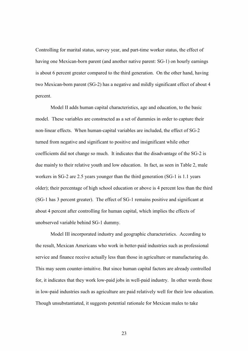
Controlling for marital status, survey year, and part-time worker status, the effect of

having one Mexican-born parent (and another native parent: SG-1) on hourly earnings

is about 6 percent greater compared to the third generation. On the other hand, having

two Mexican-born parent (SG-2) has a negative and mildly significant effect of about 4

percent.

Model II adds human capital characteristics, age and education, to the basic

model. These variables are constructed as a set of dummies in order to capture their

non-linear effects. When human-capital variables are included, the effect of SG-2

turned from negative and significant to positive and insignificant while other

coefficients did not change so much. It indicates that the disadvantage of the SG-2 is

due mainly to their relative youth and low education. In fact, as seen in Table 2, male

workers in SG-2 are 2.5 years younger than the third generation (SG-1 is 1.1 years

older); their percentage of high school education or above is 4 percent less than the third

(SG-1 has 3 percent greater). The effect of SG-1 remains positive and significant at

about 4 percent after controlling for human capital, which implies the effects of

unobserved variable behind SG-1 dummy.

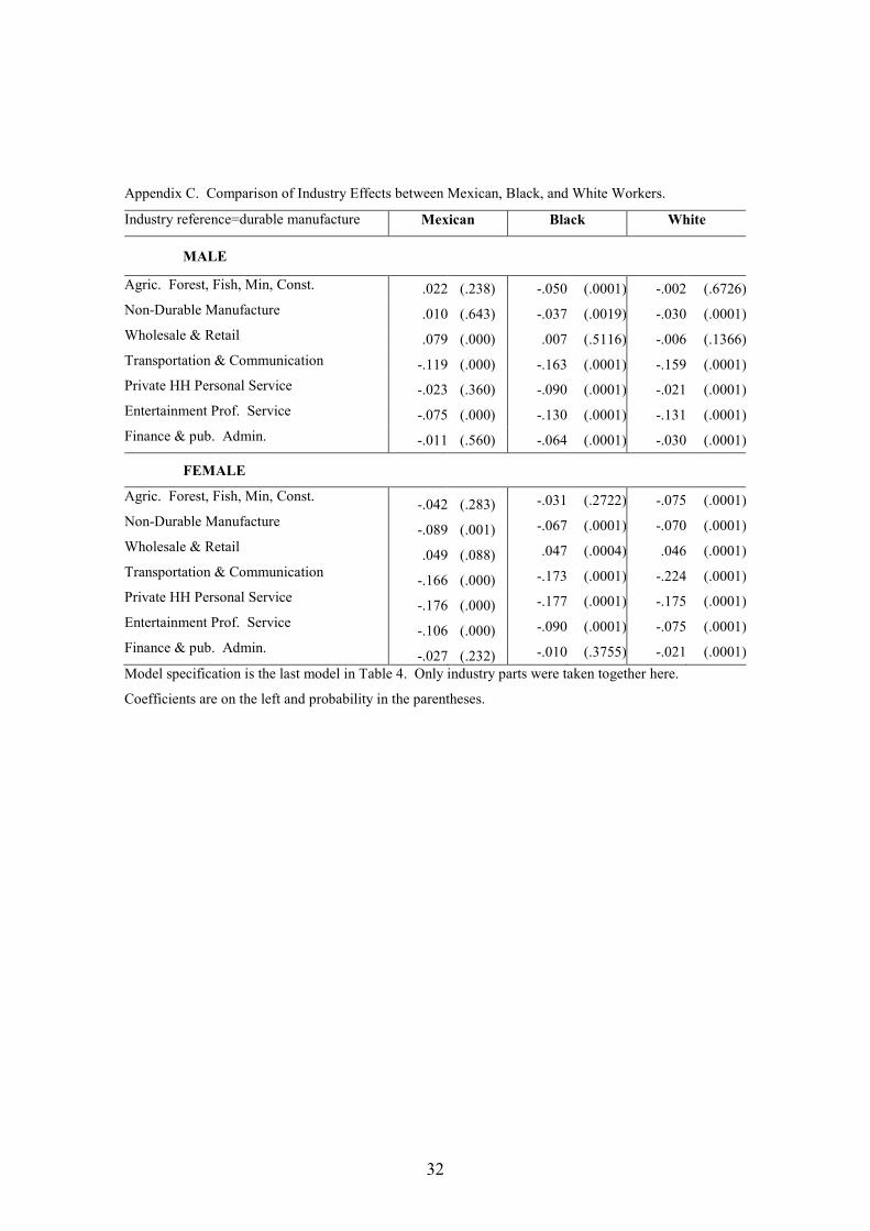
Model III incorporated industry and geographic characteristics. According to

the result, Mexican Americans who work in better-paid industries such as professional

service and finance receive actually less than those in agriculture or manufacturing do.

This may seem counter-intuitive. But since human capital factors are already controlled

for, it indicates that they work low-paid jobs in well-paid industry. In other words those

in low-paid industries such as agriculture are paid relatively well for their low education.

Though unsubstantiated, it suggests potential rationale for Mexican males to take

24

agricultural and non-durable manufacturing jobs, because these industries pay well for

their low education. In case of males, we found that native blacks and whites do not

have this pattern that Mexicans have: that is, their earnings controlling for human

capital decline if they take agricultural or non-durable manufacturing jobs (see

Appendix C). Probably, this indicates that blacks and whites are now overqualified for

these jobs.

Geographic characteristic turned out to be important determinants of earnings.

Though we cannot clarify “Not identified” and “Missing” areas, central cities and

suburbs (Balance on MSA) show clearly positive effects over those living in non-Metro

(rural) areas. Regions in the U.S. are not significant factors except for the residents in

California (+10 percent) and Texas (-9%). It should be noted that because the

coefficients for SG-1 and SG-2 have opposite direction, if we did not distinguish these

two groups, the effect of the second generation in general would be slightly positive and

insignificant. So far as Mexican male workers are concerned, the curvilinear theory had

applicability only to the SG-1 group only and their advantage may depend not on their

Mexican heritage but on native factors of their parent.

Table 5b displays the same series of regression models for female Mexican

workers. The most striking difference between the two sexes is that for female workers,

the effect of SG-1 disappeared in the model III. Although we cannot specify the reason,

the advantage of having one native parent (which could be English, motivation, legal

status, etc) does not exist for Mexican women. Given that the effect of SG-2 is also

insignificant in the model III, the earnings differences among the three groups of

Mexican female workers are completely explained away by human capital, industry and

geographic factors.

25

Conclusion

In this research on Mexican-American workers, we have clarified and combined the two

concepts: intergenerational progress and foreign-born parentage. First, we narrowed the

issue of intergenerational change to the matter between second and third generations

because the advancement from foreign-born to native-born is too obvious. Three paths

were conceptualized: linear progress, decline (curvilinear), or stagnant. We supported

the stagnation view because we hypothesized that Mexican Americans are experiencing

the segmented assimilation.

Secondly, we pointed out that the widely used definition of second generation

(at least one parent is foreign-born) might confound the effect of foreign-born parent

and native-born parent, or their combination. Having one native parent can be quite

advantageous compared with having two Mexican-born parents, or even better than

having two native-born parents. Our multivariate analysis revealed that, especially in

case of Mexican males, having two Mexican-born parents and having two native-born

parents do not make much difference if other factors are constant, while having one

Mexican parent does make positive difference. In case of females, we found little

advantage of single-Mexican parentage, and neither the difference between second and

third generations.

In sum, we do not find indication of immigrant optimism transmitted to the next

generation in any case but male workers with one Mexican-born parent (SG-1). When

both parents are foreign born (SG-2), there is no trace of such transmission. It does not

happen in any case of female workers. Unlike the literature of immigrant optimism and

curvilinear theory predicts, positive transmission of something (maybe motivation) from

26

immigrant parent seems to happen only when children is male and one of the parents is

native-born. We do not know if it is a foreign parentage or native parentage, or their

combination that brings the positive effect on earnings as we have seen in Table 4a. In

our best guess, “Mixed” nativity of Mexican parents provides male Mexican workers

with most advantage because such couples can combine the advantages of a native-born

and foreign-born to support their children. “Unmixed” foreign-born or native parents

cannot compensate each other’s disadvantage: the former is deficient in English and

legal status, and the latter causes over-assimilation to the lower class (segmented

assimilation).

Past research concluded that positive outcome is expected when foreign-born

parents and native children are “mixed” in one family, but our analysis found it is rather

mixed nativity of parents that brings about better outcomes in their children’s success.

It is important that we found such positive outlook, though it is limited, in Mexican-

American workers who might otherwise be trapped in the loop of poverty. About half

of our sample of the second generation is such family with one Mexican-born parent.

Their effort and continuous mixture of nativity can be one way to diversify their

socioeconomic stratification, which will “de-segmentize” their routes of assimilation.

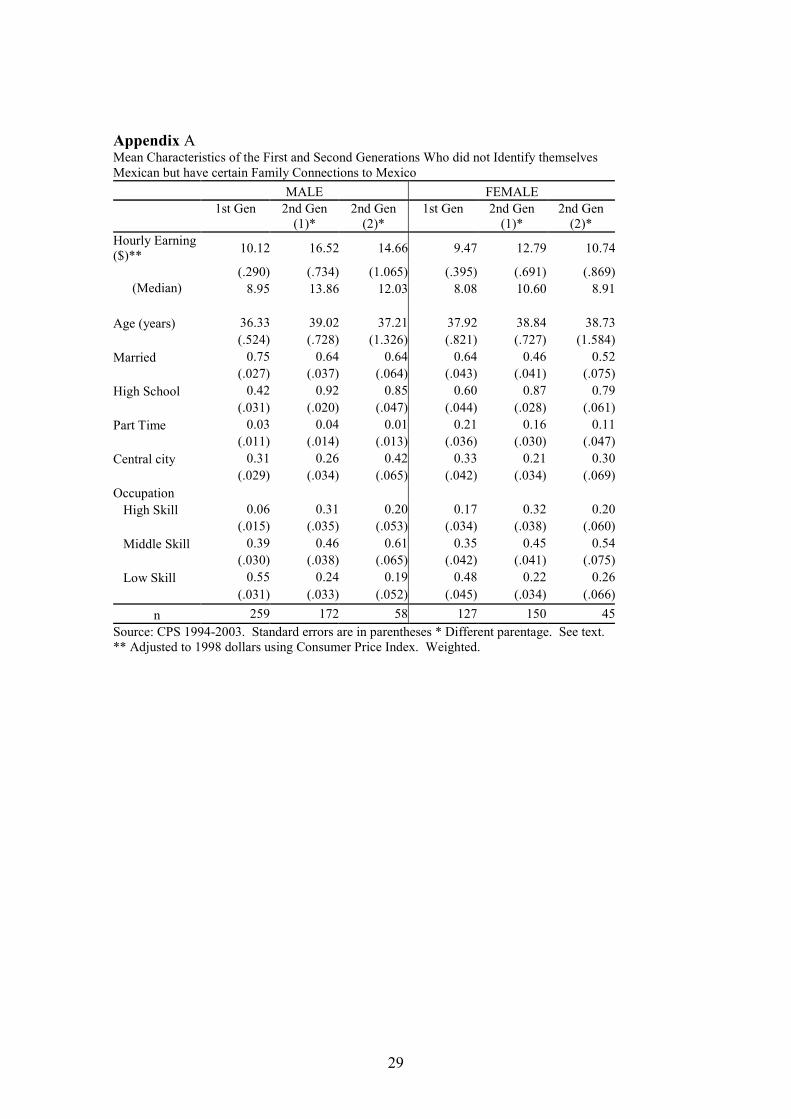
Lastly, we could not elaborate on the issue of non-self-identified Mexicans due

to its small size and lack of information. Since it is expected that a children of “mixed”

Mexican parents may abandon their Mexican identity, we should find better data and

new approach to identify them in our future research, and compare them with those

groups studied in this paper.

27

Bibliography

Borjas, George J. 1993. “The Intergenerational Mobility of Immigrants,” Journal of Labor Economics, 11-1: 113-135. Borjas, George J. 1995. “Assimilation and Changes in Cohort Quality Revisited: What Happened to Immigrant Earnings in the 1980s?” Journal of Labor Economics, 13-2: 201-245. Census Bureau 1998. “How Well Does the Current Population Survey Measure the Foreign-Born Population in the United States.” by A. Dianne Schmidley and J. Gregory Robinson. Census Bureau 2001. The Hispanic Population. Census 2000 Brief. Census Bureau 2002. Design and Methodology. Current Population Survey Technical Paper 63RV. Duncan, Brian and Stephen J. Trejo. 2004. "Ethnic Choices and the Intergenerational Progress of Mexican Americans." Working Paper Series 2004-2005, No 04-05-02. Population Research Center, University of Texas at Austin. Gans, H.J. 1992. "Second Generation Decline: Scenarios for the Economic and Ethnic Futures of Post-1965 American Immigrants." Ethnic and Racial Studies, 15: 173-192. Grogger, Jefferey and Trejo, Stephen J. 2002. Falling Behind or Moving Up?: The Intergenerational Progress of Mexican Americans. California: Public Policy Institute of California. Hernández-Léon, R. and V. Zúñiga. 2000. “Making Carpet by the Mile”: The Emergence of a Mexican Immigrant Community in an Industrial Region of the U.S. Historic South.” Social Science Quarterly 81(1): 49-66. Hernández-León, R. and V. Zúñiga. 2004. “Mexican Immigrant Communities in the South and Social Capital: The Case of Dalton, Georgia.” Southern Rural Sociology 19(2), forthcoming Kao, Grace and Tienda Marta, 1995. "Optimism and Achievement: The Educational Performance of Immigrant Youth." Social Science Quarterly 76 1, pp 1-19. Kao, Grace and Jennifer Thompson. 2003.“Race and Ethnic Stratification in Educational Achievement and Attainment.”Annual Review of Sociology. 29: 417-442. Pong, Suet-ling. 2003 “Immigrant Children's School Performance” Working Paper 03-07, Population Research Institute, The Pennsylvania State University

28

Portes, Alejandro and Lingxin Hao. 2004. “The Schooling of Children of Immigrants: Contextual Effects on the Educational Attainment of the Second Generation.” Proceeding of National Academy of Science 101:11920-27. Portes, Alejandro and Rumbaut, Rubén G. 2001. Legacies: The Story of the Immigrant Second Generation. Berkeley and New York: University of California Press. Smith, JP. 2003. “Assimilation across the Latino Generations” American Economic Review 93: 315-319 Trejo, Stephen J. 1997. “Why Do Mexican Earn Low Wages?” The Journal of Political Economy, 105(6):1235-1268. Waldinger, Roger and Perlmann, Joel. "Are the Children of Today's Immigrants Making It?", The Public Interest, Number 132, Summer 1998, pp. 73-96.

29

Appendix A Mean Characteristics of the First and Second Generations Who did not Identify themselves Mexican but have certain Family Connections to Mexico

MALE FEMALE

1st Gen 2nd Gen

(1)* 2nd Gen (2)*

1st Gen 2nd Gen (1)*

2nd Gen (2)*

Hourly Earning ($)**

10.12 16.52 14.66 9.47 12.79 10.74

(.290) (.734) (1.065) (.395) (.691) (.869)

(Median) 8.95 13.86 12.03 8.08 10.60 8.91

Age (years) 36.33 39.02 37.21 37.92 38.84 38.73

(.524) (.728) (1.326) (.821) (.727) (1.584)

Married 0.75 0.64 0.64 0.64 0.46 0.52

(.027) (.037) (.064) (.043) (.041) (.075)

High School 0.42 0.92 0.85 0.60 0.87 0.79

(.031) (.020) (.047) (.044) (.028) (.061)

Part Time 0.03 0.04 0.01 0.21 0.16 0.11

(.011) (.014) (.013) (.036) (.030) (.047)

Central city 0.31 0.26 0.42 0.33 0.21 0.30

(.029) (.034) (.065) (.042) (.034) (.069)

Occupation

High Skill 0.06 0.31 0.20 0.17 0.32 0.20

(.015) (.035) (.053) (.034) (.038) (.060)

Middle Skill 0.39 0.46 0.61 0.35 0.45 0.54

(.030) (.038) (.065) (.042) (.041) (.075)

Low Skill 0.55 0.24 0.19 0.48 0.22 0.26

(.031) (.033) (.052) (.045) (.034) (.066)

n 259 172 58 127 150 45

Source: CPS 1994-2003. Standard errors are in parentheses * Different parentage. See text. ** Adjusted to 1998 dollars using Consumer Price Index. Weighted.

30

Appendix B: Industrial and Occupational Distribution of Mexicans, Blacks and Whites

(1) MALE Mexican Mexican Mexican Mexican Native Native

INDUSTRY 1st Gen 2nd Gen

(1)* 2nd Gen (2)*

3rd Gen NH Black

NH White

Agriculture 11.86 2.48 4.33 2.37 1.08 1.28

Mining 0.56 1.34 1.25 1.86 0.38 1.46

Construction 18.76 9.84 12.08 12.04 7.16 10.06

Manufacturing - Durable Goods 14.8 12.7 12.33 12.33 13.32 15.89

Mfg. - Non-Durable Goods 11.99 9.74 9.58 9.37 9.64 8.86

Transportation 3.43 8.12 7.25 7.45 10.88 7.02

Communications 0.31 2.29 2.25 1.86 1.99 2.07

Utilities And Sanitary Services 0.68 3.06 2.5 3.2 2.69 2.92

Wholesale Trade 5.11 6.4 6.67 5.83 4.26 6.1

Retail Trade 14.64 10.41 12.58 12.73 11.42 11.08

Finance, Insurance, And Real Estate 3.53 3.63 3.25 4.07 4.43 5.01

Private Households 0.96 1.05 0.58 0.92 0.46 0.42

Business, Auto And Repair Services 5.92 6.69 6.33 6.96 7.19 6.22

Personal Services, Exc. Private Hhlds 2.79 1.43 1.92 1.14 1.76 1.05

Entertainment And Recreation Services 1.31 0.86 1.42 1.32 1.21 1.23

Hospitals 0.42 2.01 1.92 1.45 2.92 1.81

Medical Services, Exc. Hospitals 0.43 1.91 1.17 1.09 1.61 1.33

Educational Services 1.19 5.73 4.25 4.66 5.23 5.31

Social Services 0.21 0.76 1 0.99 2 0.68

Other Professional Services 0.49 2.39 1.92 2.25 2.44 4.03

Forestry And Fisheries 0.1 0.1 . 0.09 0.04 0.17

Public Administration 0.53 7.07 5.42 6.02 7.89 6.02

All 100 100 100 100 100 100

OCCUPATION

Executive, Admin, & Managerial 2.71 10.79 7.83 9.4 9.2 16.84

Professional Specialty 1.66 9.65 8.83 8.83 9.79 15.73

Technicians And Related Support 3.78 3.72 4.17 5.45 3.84 4.16

Sales 2.9 8.12 6.5 7.91 5.67 10.75

Administrative Support, Including Clerical

2.81 7.83 9.58 7.64 9.34 5.68

Private Household 0.92 0.29 0.25 0.2 0.1 0.1

Protective Service 3.49 4.58 4.5 5.65 5.61 3.89

Service, Excluding Protective & Household

14.62 6.11 7.92 7.84 10.36 4.43

Precision Prod., Craft & Repair 23.1 20.44 20.17 20.56 14.83 19.55

Machine Operators, Assemblers & Inspectors

14.88 9.46 9.75 8.56 11.3 7.04

Transportation And Material Moving 6.04 9.65 8.08 8.32 10.67 6.78

Handlers, Equipment Cleaners, Helpers, Laborers

11.29 6.4 7.67 6.88 7.7 3.62

Farming, Forestry And Fishing 11.81 2.96 4.75 2.76 1.58 1.43

All 100 100 100 100 100 100

31

(2) FEMALE Mexican Mexican Mexican Mexican Native Native

INDUSTRY 1st Gen 2nd Gen

(1)* 2nd Gen (2)*

3rd Gen NH Black

NH White

Agriculture 3.75 0.53 1.07 0.54 0.15 0.67

Mining 0.04 . 0.18 0.23 0.06 0.22

Construction 0.61 1.17 0.89 0.98 0.51 1.35

Manufacturing - Durable Goods 12.31 5.95 5.53 6.16 5.75 6.18

Mfg. - Non-Durable Goods 17.64 5.53 8.02 6.56 6.8 6.07

Transportation 1.27 2.34 3.83 2.72 4.27 2.75

Communications 0.39 1.49 1.96 2.16 2.25 1.55

Utilities And Sanitary Services 0.5 1.06 1.52 2.14 1.52 1.66

Wholesale Trade 4.72 2.66 4.37 4.07 1.93 3.25

Retail Trade 16.02 15.41 15.86 19.71 13.23 17.09

Finance, Insurance, And Real Estate 5.29 7.55 9.45 7.63 7.55 8.92

Private Households 7.02 1.38 1.34 1.33 1.37 0.93

Business, Auto And Repair Services 5.02 4.36 4.55 4.59 5.61 4.28

Personal Services, Exc. Private Hhlds 8.78 3.19 3.74 2.93 2.8 2.09

Entertainment And Recreation Services 0.83 0.53 0.36 1.1 0.81 1.12

Hospitals 2.19 4.68 4.99 4.94 8.51 7.28

Medical Services, Exc. Hospitals 4.01 7.97 7.13 8.2 8.89 8.34

Educational Services 5.11 18.49 12.66 12.01 11.25 13.78

Social Services 2.55 4.99 3.48 3.73 5.24 3.08

Other Professional Services 0.92 4.25 3.12 2.37 2.65 4.63

Forestry And Fisheries 0.02 . 0.09 0.06 0.03 0.08

Public Administration 1.05 6.48 5.88 5.81 8.81 4.69

All 100 100 100 100 100 100

OCCUPATION

Executive, Admin, & Managerial 3.75 13.28 12.48 12.53 11.78 16.49

Professional Specialty 3.67 15.62 13.64 13.82 15.88 22.67

Technicians And Related Support 6.14 6.59 6.51 7.08 5.69 5.54

Sales 6.72 9.46 8.82 10.62 7.54 10.27

Administrative Support, Including Clerical

10.12 29.44 33.51 29.94 25.94 26.23

Private Household 5.93 0.85 0.89 0.79 0.82 0.46

Protective Service 0.31 1.28 0.8 0.71 1.7 0.53

Service, Excluding Protective & Household

24.31 12.96 12.03 13.49 17.49 9.64

Precision Prod., Craft & Repair 7.55 3.08 1.96 3.46 2.68 2.17

Machine Operators, Assemblers & Inspectors

21.66 4.57 5.7 4.48 6.96 3.48

Transportation And Material Moving 0.46 0.74 0.98 0.97 1.37 0.87

Handlers, Equipment Cleaners, Helpers, Laborers

4.91 1.59 2.05 1.64 2 1.27

Farming, Forestry And Fishing 4.46 0.53 0.62 0.46 0.16 0.38

All 100 100 100 100 100 100

32

Appendix C. Comparison of Industry Effects between Mexican, Black, and White Workers.

Industry reference=durable manufacture Mexican Black White

MALE

Agric. Forest, Fish, Min, Const. .022 (.238) -.050 (.0001) -.002 (.6726)

Non-Durable Manufacture .010 (.643) -.037 (.0019) -.030 (.0001)

Wholesale & Retail .079 (.000) .007 (.5116) -.006 (.1366)

Transportation & Communication -.119 (.000) -.163 (.0001) -.159 (.0001)

Private HH Personal Service -.023 (.360) -.090 (.0001) -.021 (.0001)

Entertainment Prof. Service -.075 (.000) -.130 (.0001) -.131 (.0001)

Finance & pub. Admin. -.011 (.560) -.064 (.0001) -.030 (.0001)

FEMALE

Agric. Forest, Fish, Min, Const. -.042 (.283) -.031 (.2722) -.075 (.0001)

Non-Durable Manufacture -.089 (.001) -.067 (.0001) -.070 (.0001)

Wholesale & Retail .049 (.088) .047 (.0004) .046 (.0001)

Transportation & Communication -.166 (.000) -.173 (.0001) -.224 (.0001)

Private HH Personal Service -.176 (.000) -.177 (.0001) -.175 (.0001)

Entertainment Prof. Service -.106 (.000) -.090 (.0001) -.075 (.0001)

Finance & pub. Admin. -.027 (.232) -.010 (.3755) -.021 (.0001)

Model specification is the last model in Table 4. Only industry parts were taken together here.

Coefficients are on the left and probability in the parentheses.