
Generation of seamless transitions between 2D and...
47
IT 10 033 Examensarbete 30 hp Juni 2010 Generation of seamless transitions between 2D and 3D geometries Gustavo Torres Institutionen för informationsteknologi Department of Information Technology
Transcript of Generation of seamless transitions between 2D and...

IT 10 033
Examensarbete 30 hpJuni 2010
Generation of seamless transitions between 2D and 3D geometries
Gustavo Torres
Institutionen för informationsteknologiDepartment of Information Technology


Teknisk- naturvetenskaplig fakultet UTH-enheten Besöksadress: Ångströmlaboratoriet Lägerhyddsvägen 1 Hus 4, Plan 0 Postadress: Box 536 751 21 Uppsala Telefon: 018 – 471 30 03 Telefax: 018 – 471 30 00 Hemsida: http://www.teknat.uu.se/student
Abstract
Generation of seamless transitions between 2D and3D geometries
Gustavo Torres
There is a big gap between 2D and 3D visualization in modern computer generated graphics. It is common to see that visual representations focus either on 2D visualization (e.g. contact lists, maps, text readers, etc.) or on 3D visualization (e.g. videogames, scientific simulations, data visualization, etc.). Such heavy use of single-oriented visualizations motivated the focus on hybrid interfaces that merged the advantages of both 2D and 3D visualizations.
In order to make the gap between 2D and 3D less noticeable, smooth transitions are needed. For a transition between 2D and 3D to be smooth there should not be considerably big structural changes in the transitions. This can be accomplished if a coherent correlation exists between the 2D image and the 3D representation.
The main goal of this project is to find coherent correlations between a 2D image and a 3D mesh, which is the most common way of representing a 3D object. The correlation will be interpreted as a matching between corners in the image and vertices in the mesh. To be able to manage transitions of large input data in a feasible amount of time, approximate methods have to be used. That is why meta-heuristics were used in the search of optimal correlations.
Keywords: Computer Graphics, Transition, Two Dimensions, Three Dimensions, Meta-heuristics, Simulated Annealing, Iterated Local Search, Matching
Tryckt av: Reprocentralen ITCIT 10 033Examinator: Anders JanssonÄmnesgranskare: Stefan SeipelHandledare: Dan Gärdenfors

“The reasonable man adapts himself to the world; the unreasonable one persists in trying
to adapt the world to himself. Therefore all progress depends on the unreasonable man”
George Bernard Shaw

Acknowledgements
We would like to thank the following people for all their contributions that made possible
in one way or another to carry out our thesis successfully:
• To Tobias and Andreas who made the working environment at TAT as pleasant
as one can expect, and who became our friends in such a short time.
• To Mika for helping us at TAT with all technical questions we could come up with.
• To Dan and Michael for providing their help as our supervisors, and for trying
their best to carry on the right direction our thesis.
• To Alex, Fabio, Laura, Jonathan and Cheo for showing us that friendship is a
valuable good that could never be overestimated.
• To Cheche for making us feel like home, even when we are hundreds of kilometers
away from home.
• To Liene and Vera for always being there when we needed them, for being the
greatest party mates and friends one can find, and for never putting us on the
corner :)
• To our alma mater Universidad Simon Bolıvar for teaching us how to be excellent
at our studies, and for giving us the opportunity to do this amazing exchange year.
• And of course to our families, because of their enormous support and sacrifices so
that we can be writing our thesis right now.
v

Preface
This work was carried jointly by the author, Gustavo Torres, and by Juan Martınez
from Lund University. The author worked mainly on the implementation of the meta-
heuristics algorithms on the test cases while Martınez on the visualization of those. All
the design of the problem along with the solution was jointly carried away.
vi
Contents
Acknowledgements v
Preface vi
List of Figures ix
List of Tables x
List of Algorithms xi
Abbreviations xii
1 Introduction 1
1.1 Objectives . . . . . . . . . . . . . . . . . . . . . . . . . . . . . . . . . . . . 2
1.2 Structure . . . . . . . . . . . . . . . . . . . . . . . . . . . . . . . . . . . . 2
1.3 Previous Studies . . . . . . . . . . . . . . . . . . . . . . . . . . . . . . . . 3
2 Background 4
2.1 Meta Heuristics . . . . . . . . . . . . . . . . . . . . . . . . . . . . . . . . . 4
2.1.1 Local Search . . . . . . . . . . . . . . . . . . . . . . . . . . . . . . 6
2.1.2 Simulated Annealing . . . . . . . . . . . . . . . . . . . . . . . . . . 7
2.1.2.1 Basic concept . . . . . . . . . . . . . . . . . . . . . . . . . 7
2.1.2.2 Algorithm . . . . . . . . . . . . . . . . . . . . . . . . . . 7
2.1.3 Iterated Local Search . . . . . . . . . . . . . . . . . . . . . . . . . 8
2.2 Meshes . . . . . . . . . . . . . . . . . . . . . . . . . . . . . . . . . . . . . . 10
2.3 Images . . . . . . . . . . . . . . . . . . . . . . . . . . . . . . . . . . . . . . 11
2.3.1 Corner Detection on images . . . . . . . . . . . . . . . . . . . . . . 11
3 Tools 13
3.1 OpenCV . . . . . . . . . . . . . . . . . . . . . . . . . . . . . . . . . . . . . 13
3.2 Wavefront (OBJ) Loader . . . . . . . . . . . . . . . . . . . . . . . . . . . . 14
3.3 TAT Motion LabTM . . . . . . . . . . . . . . . . . . . . . . . . . . . . . . 14
3.4 Blender . . . . . . . . . . . . . . . . . . . . . . . . . . . . . . . . . . . . . 15
4 Meta-heuristics design 16
4.1 Problem Description . . . . . . . . . . . . . . . . . . . . . . . . . . . . . . 17
vii

Contents viii
4.2 Goal Function . . . . . . . . . . . . . . . . . . . . . . . . . . . . . . . . . . 17
4.3 Neighbor Operator . . . . . . . . . . . . . . . . . . . . . . . . . . . . . . . 19
4.4 Initial Solution . . . . . . . . . . . . . . . . . . . . . . . . . . . . . . . . . 20
4.5 Meta-heuristics implemented . . . . . . . . . . . . . . . . . . . . . . . . . 20
4.5.1 Local Search: First improvement . . . . . . . . . . . . . . . . . . . 20
4.5.2 Local Search: Best improvement . . . . . . . . . . . . . . . . . . . 20
4.5.3 Simulated annealing . . . . . . . . . . . . . . . . . . . . . . . . . . 21
4.5.4 Iterated Local Search . . . . . . . . . . . . . . . . . . . . . . . . . 21
5 Development and Results 22
5.1 Development . . . . . . . . . . . . . . . . . . . . . . . . . . . . . . . . . . 22
5.2 Results . . . . . . . . . . . . . . . . . . . . . . . . . . . . . . . . . . . . . . 22
5.3 Discussion . . . . . . . . . . . . . . . . . . . . . . . . . . . . . . . . . . . . 24
5.3.1 Plane . . . . . . . . . . . . . . . . . . . . . . . . . . . . . . . . . . 25
5.3.2 Cross . . . . . . . . . . . . . . . . . . . . . . . . . . . . . . . . . . 27
5.3.3 Map . . . . . . . . . . . . . . . . . . . . . . . . . . . . . . . . . . . 29
5.3.4 Dodecahedron . . . . . . . . . . . . . . . . . . . . . . . . . . . . . 30
5.3.5 Map Demo . . . . . . . . . . . . . . . . . . . . . . . . . . . . . . . 30
6 Conclusion 32
6.1 Recommendations for Future Research . . . . . . . . . . . . . . . . . . . . 32
Bibliography 34

List of Figures
2.1 Graphical comparison between annealing and quenching . . . . . . . . . . 8
2.2 Pictorial representation of ILS . . . . . . . . . . . . . . . . . . . . . . . . 9
2.3 Triangle mesh representing a dolphin . . . . . . . . . . . . . . . . . . . . 11
2.4 Applied edge detection . . . . . . . . . . . . . . . . . . . . . . . . . . . . 12
2.5 Applied corner detection . . . . . . . . . . . . . . . . . . . . . . . . . . . 12
4.1 2D input image that will be used in the problem with detected cornershighlighted . . . . . . . . . . . . . . . . . . . . . . . . . . . . . . . . . . . 16
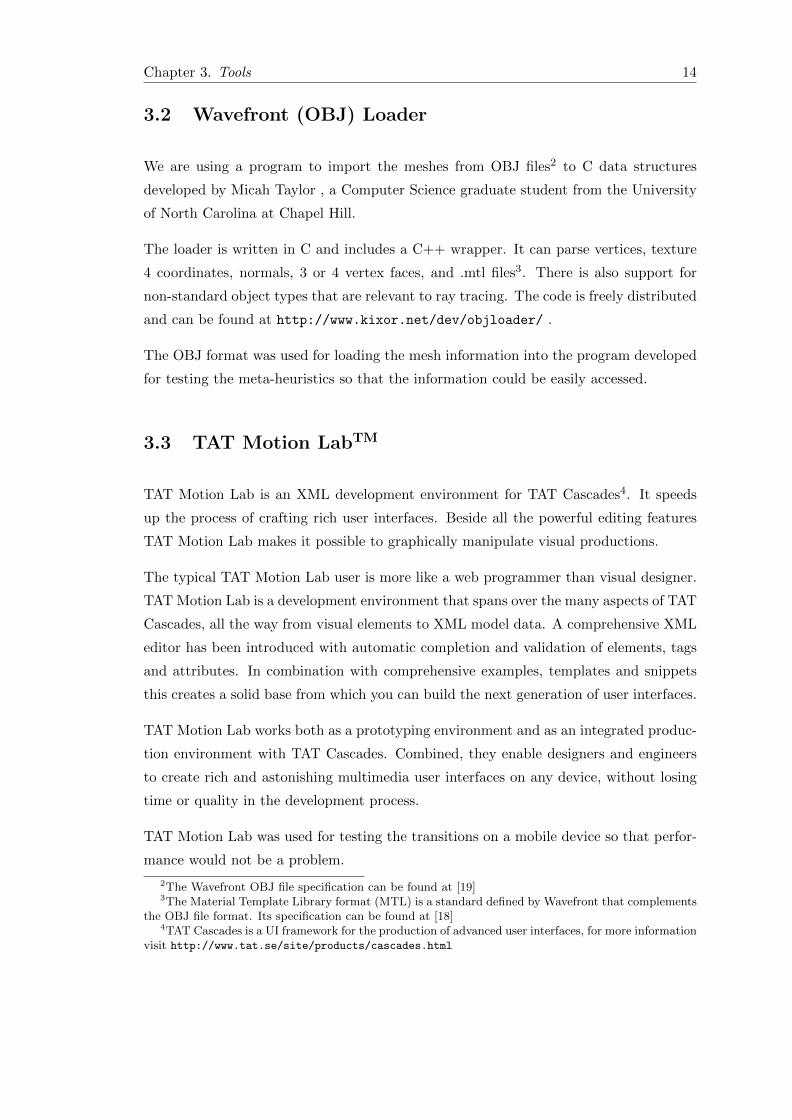
4.2 3D mesh corresponding to the the 2D image shown on Figure 4.1 . . . . 17
5.1 Plane input image used for running the Plane test-case . . . . . . . . . . 23
5.2 Cross input image used for running the Cross test-case . . . . . . . . . . 23
5.3 Map input image used for running the Map test-case . . . . . . . . . . . 24
5.4 Dodecahedron input image used for the Dodecahedron test-case . . . . . . 24
5.5 Plane input mesh used for the Plane test-case . . . . . . . . . . . . . . . 25
5.6 Cross input mesh used for the Cross test-case . . . . . . . . . . . . . . . 25
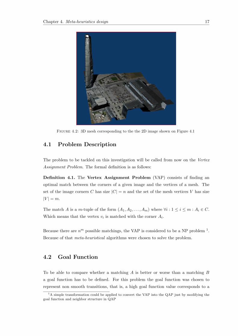
5.7 Map input mesh used for the Map test-case . . . . . . . . . . . . . . . . . 26
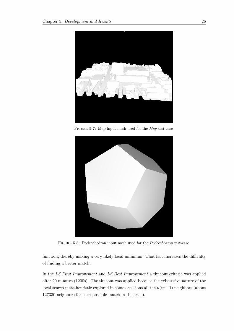
5.8 Dodecahedron input mesh used for the Dodecahedron test-case . . . . . . 26
5.9 Best Plane matching returned in the Plane test-case . . . . . . . . . . . . 27
5.10 Best Cross matching returned in the Cross test-case . . . . . . . . . . . . 27
5.11 Best Map matching returned in the Map test-case . . . . . . . . . . . . . 28
5.12 Best Dodecahedron matching returned in the Dodecahedron test-case . . 28
5.13 Animation on the Cross test-case using ω1 = 1 and ω2 = 0 . . . . . . . . 29
5.14 Smooth transition between 2D and 3D maps . . . . . . . . . . . . . . . . 31
ix

List of Tables
2.1 Analogies between Annealing and the SA Meta-heuristic . . . . . . . . . . 7
5.1 Goal function results and times for the three test-cases tried . . . . . . . . 23
x

List of Algorithms
2.1 Local search . . . . . . . . . . . . . . . . . . . . . . . . . . . . . . . . . . . 6
2.2 Simulated Annealing . . . . . . . . . . . . . . . . . . . . . . . . . . . . . . 9
2.3 Iterated Local Search . . . . . . . . . . . . . . . . . . . . . . . . . . . . . . 10
5.1 Framework used for testing . . . . . . . . . . . . . . . . . . . . . . . . . . 22
xi

Abbreviations
2D Two Dimensions
3D Three Dimensions
CO Combinatorial Optimization
ILS Iterated Local Search
LS Local Search
SA Simulated Annealing
TAT The Astonishing Tribe
TSP Traveling Salesman Problem
QAP Quadratic Assignment Problem
UI User Interface
VAP Vertex Assignment Problem
VRP Vehicle Routing Problem
xii

“Beauty is a good letter of
introduction.”
German proverb
Chapter 1
Introduction
The representation of different types of computer generated images in digital displays
have gained a lot of relevance in many areas, such as scientific simulations, videogames,
user interfaces, data visualization, graphical design, among others; which has drawn
plenty of attention from computer scientists and companies to improve them in order to
make them more aesthetic, useful and give a better experience to the user.
Broadly speaking, computer graphics is concerned with “all aspects of producing pictures
or images using a computer” [1]. Its origins are considered to be in the year 1961 when
Ivan Sutherlan, a student from MIT, developed a drawing program that consisted on
a pen which transmitted electronic impulses that could generate very simple lines on a
cathode-ray tube (CRT) screen. From that point, the improvements on this field have
been guided by the development of new technologies on the devices used and by the
discovery of new and more efficient algorithms to generate such graphical representations.
These advances in computer graphics have been characterized as well by a closer repre-
sentation of reality with the introduction of three dimensional graphics. The improve-
ments have been that big, that sometimes the images generated are indistinguishable
from the real phenomena they are trying to depict, turning computer graphics into a
factor of vital importance for a lot of the fields on which they are used.
Despite the fact that newer and generally more appealing graphic paradigms (mainly
3D graphics) unveiled from the improvements in algorithms and hardware, there is a
considerable portion of the users that still prefer the plain and simple 2D paradigm.
This preference might seem strange for some, but the reason behind it is that both of
these paradigms, 2D and 3D graphics, offer a different experience to the users and some
applications may be benefited more from one than the other, while others could take
advantage of both of them.
1

Chapter 1. Introduction 2
Among the aspects that make 2D graphics more attractive for some users, we can find:
simplicity, readability and abstraction; which make them more suitable for applications
such as: text editors, email applications, 2D design, information organization, interac-
tive menus, web browsing, flat data visualization, etc. On the other hand, 3D graphics
present some other characteristics described in previous studies [15], like: realism, flex-
ible information visualization, naturalized interaction, visual style, and feedback. Fea-
tures that make them suitable for applications such as: videogames, physics engines,
3D design, simulation, modern user interfaces, special effects, and augmented reality,
among others.
This separation of preferences is our main motivation for doing this thesis; to make it
possible to have the best of both worlds without losing track of the relation between one
and the other, that is, to create seamless transitions between 2D and 3D graphics
In order to accomplish that goal in an efficient way, we used known computational
methods known as meta-heuristics, which allowed us to find adequate matchings between
the corners of 2D images and the vertices of 3D images in a reasonable time, even for
large test cases.
1.1 Objectives
The specific goals for this project are:
• Design of different heuristics for matching polygonal mesh vertices with bi-dimensional
image points for the interactive generation of seamless transitions between 2D and
3D.
• Comparison of different heuristics for matching polygonal mesh vertices with bi-
dimensional image points for the interactive generation of seamless transitions
between 2D and 3D.
• Creation of a graphics simulator for testing the different implemented heuristics.
1.2 Structure
This thesis report is structured by the following chapters:
• Background: An overview of the theoretic content used throughout the thesis
report is offered.

Chapter 1. Introduction 3
• Tools: The different tools that helped us on the development of the project are
described.
• Meta-heuristics design: We give a detailed description of the design and adaptation
of the two meta-heuristics used.
• Development and Results: The programming environment and the testing process
are described here, followed by the results discussion.
1.3 Previous Studies
In the literature there are some references about transitions between two 3D meshes
given in different ways. Although no specific study was found about creating mesh for
doing transitions between 2D images and 3D meshes.
The main difference between this work and the previous found, is that this work focuses
on finding a good representation of a 2D image as 3D mesh for doing the transition;
meanwhile previous studies main focus is on exploring different transitions between two
already known 3D meshes.

“Admiration for a quality or an art
can be so strong that it deters us from
striving to possess it.”
Friedrich Nietzsche
Chapter 2
Background
In this chapter there will be a theoretical background that will settle all the definitions
and technical terms that will be used through the thesis. Through the development
of this investigation, a deep understanding of meta-heuristics, meshes, image represen-
tations and image analysis was required. Some of the concepts from those areas are
presented in this chapter before using them in the rest of the text.
2.1 Meta Heuristics
According to El-Ghazali[4] the word heuristic has its origin from the Greek word heuriskein,
which means “the art of discovering new strategies (rules) to solve problems”, and the
suffix meta, also a Greek word, means “upper level methodology”. In short, meta-
heuristics are a methodology for discovering new strategies to solve problems.
In computer science, according to Luke Sean[17], meta heuristics are a common term
used to refer to describe the major field of stochastic optimization, which is the
general class of algorithms and techniques that employ randomness to find optimal (or
near optimal) solutions to hard combinatorial problems.
More specifically, a meta-heuristic is a framework used to solve a broad selection of
combinatorial optimization problems in a feasible amount of time. According to Blum
et al.[2]:
Definition 2.1. A Combinatorial Optimization (CO) problem P = (S, f) can be defined
by:
• a set of variables X = {x1, . . . , xn}
4
Chapter 2. Background 5
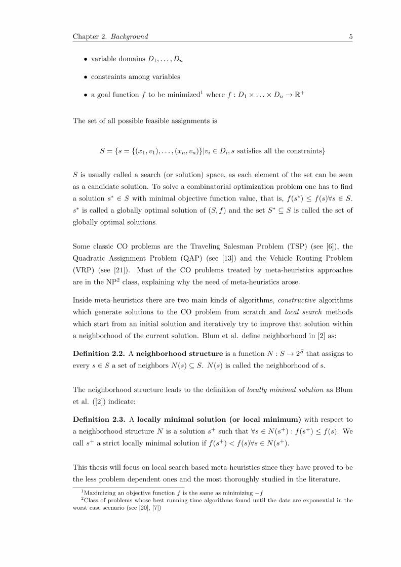
• variable domains D1, . . . , Dn
• constraints among variables
• a goal function f to be minimized1 where f : D1 × . . .×Dn → R+
The set of all possible feasible assignments is
S = {s = {(x1, v1), . . . , (xn, vn)}|vi ∈ Di, s satisfies all the constraints}
S is usually called a search (or solution) space, as each element of the set can be seen
as a candidate solution. To solve a combinatorial optimization problem one has to find
a solution s∗ ∈ S with minimal objective function value, that is, f(s∗) ≤ f(s)∀s ∈ S.
s∗ is called a globally optimal solution of (S, f) and the set S∗ ⊆ S is called the set of
globally optimal solutions.
Some classic CO problems are the Traveling Salesman Problem (TSP) (see [6]), the
Quadratic Assignment Problem (QAP) (see [13]) and the Vehicle Routing Problem
(VRP) (see [21]). Most of the CO problems treated by meta-heuristics approaches
are in the NP2 class, explaining why the need of meta-heuristics arose.
Inside meta-heuristics there are two main kinds of algorithms, constructive algorithms
which generate solutions to the CO problem from scratch and local search methods
which start from an initial solution and iteratively try to improve that solution within
a neighborhood of the current solution. Blum et al. define neighborhood in [2] as:
Definition 2.2. A neighborhood structure is a function N : S → 2S that assigns to
every s ∈ S a set of neighbors N(s) ⊆ S. N(s) is called the neighborhood of s.
The neighborhood structure leads to the definition of locally minimal solution as Blum
et al. ([2]) indicate:
Definition 2.3. A locally minimal solution (or local minimum) with respect to
a neighborhood structure N is a solution s+ such that ∀s ∈ N(s+) : f(s+) ≤ f(s). We
call s+ a strict locally minimal solution if f(s+) < f(s)∀s ∈ N(s+).
This thesis will focus on local search based meta-heuristics since they have proved to be
the less problem dependent ones and the most thoroughly studied in the literature.
1Maximizing an objective function f is the same as minimizing −f2Class of problems whose best running time algorithms found until the date are exponential in the
worst case scenario (see [20], [7])
Chapter 2. Background 6
2.1.1 Local Search
Almost all meta-heuristics follow the same pattern of behavior when they are searching
for a near optimal solution. I.e. they start in some part of the search space (S) and
then they keep moving through it, using the neighborhood structure (see definition 2.2)
designed for the CO problem.
In order to be able to start exploring the search space S, an initial solution is needed.
Definition 2.4. An initial solution to a CO problem is an arbitrary chosen solution
to the CO problem. It could be generated randomly or with some kind of heuristic to
improve the performance of the meta-heuristics. This initial solution can be seen as a
function init : ∅ → S that generates solutions without receiving any kind of input.
According to Hoos et al.[9] Local Search meta-heuristics are defined as:
Definition 2.5. The Local Search meta-heuristic is defined by the following compo-
nents:
• a step function step : S → S mapping the actual solution into a solution in the
neighborhood structure.
• a termination predicate that determines when the search for solutions to the CO
problem has ended.
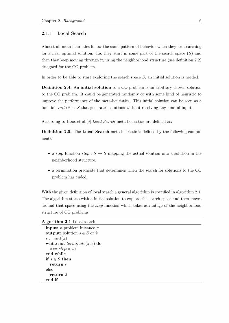
With the given definition of local search a general algorithm is specified in algorithm 2.1.
The algorithm starts with a initial solution to explore the search space and then moves
around that space using the step function which takes advantage of the neighborhood
structure of CO problems.
Algorithm 2.1 Local search
input: a problem instance πoutput: solution s ∈ S or ∅s := init(π)while not terminate(π, s) dos := step(π, s)
end whileif s ∈ S then
return selse
return ∅end if

Chapter 2. Background 7
2.1.2 Simulated Annealing
2.1.2.1 Basic concept
Simulated Annealing (SA) is a nature inspired meta-heuristic that simulates a physical
phenomena heavily studied in material science. Dreo et al. provide a good definition of
annealing in [10]
The annealing technique consists in heating a material beforehand to im-
part high energy to it. Then the material is cooled slowly, by keeping at
each stage a temperature of sufficient duration; if the decrease in temper-
ature is too fast, it may cause defects which can be eliminated by local re-
heating. This strategy of a controlled decrease of the temperature leads to a
crystallized solid state, which is a stable state, corresponding to an absolute
minimum of energy. The opposite technique is that of the quenching, which
consists in very quickly lowering the temperature of the material: this can
lead to an amorphous structure, a metastable state that corresponds to a lo-
cal minimum of energy. In the annealing technique the cooling of a material
caused a disorder-order transformation, while the quenching was responsible
in solidifying a disordered state.
A graphical representation of these two phenomena can be seen on Figure 2.1 taken from
[10].
The analogy between CO problem and the annealing process comes from the fact that
a minimum energy state can be directly compared with a minimum goal function value
as seen in Table 2.1 (from [10]).
Optimization Problem Physical system
objective function free energyparameters of the problem “coordinates” of the particle
find a good solution find the low energy states
Table 2.1: Analogies between Annealing and the SA Meta-heuristic
2.1.2.2 Algorithm
The CO algorithm for SA works in a very similar way to the physical phenomena. It
starts with a high temperature and an initial solution, at each temperature the algo-
rithm tries different solutions (particle states in the annealing method) and stays in
that solution with a probability depending on the temperature. At higher temperatures

Chapter 2. Background 8
Figure 2.1: Graphical comparison between annealing and quenching
the probability of taking solutions with bigger goal function values is higher, but as the
temperature decreases only better solutions are taken.
In order to be able to decide whether to take a solution at a given temperature, the
probability function e−∆E
T is used ([10]), where ∆E is the difference between the goal
function value of the current solution being explored minus the one of the previous
solution explored (∆E = f(sactual) − f(sprevious)). This function is very useful for SA
because when T (the current temperature) is very high, e−∆E
T → 1, making the algorithm
more sensitive to take worse solutions, and when T is low only better solutions will be
accepted. When a better solution is found in the SA algorithm there’s no need to use
the probability function since we are improving the energy of the system. A detailed
algorithm is found on Algorithm 2.2.
2.1.3 Iterated Local Search
Iterated Local Search (ILS) builds up onto the local search concept as specified by
Lorenco et al. in [8]. In Figure 2.2 there is a pictorial representation of how ILS behaves.
The main idea of ILS is to first start with an initial solution s0, apply a localSearch
procedure to improve the solution (s′), then apply a “perturbation” to s′ in order to be
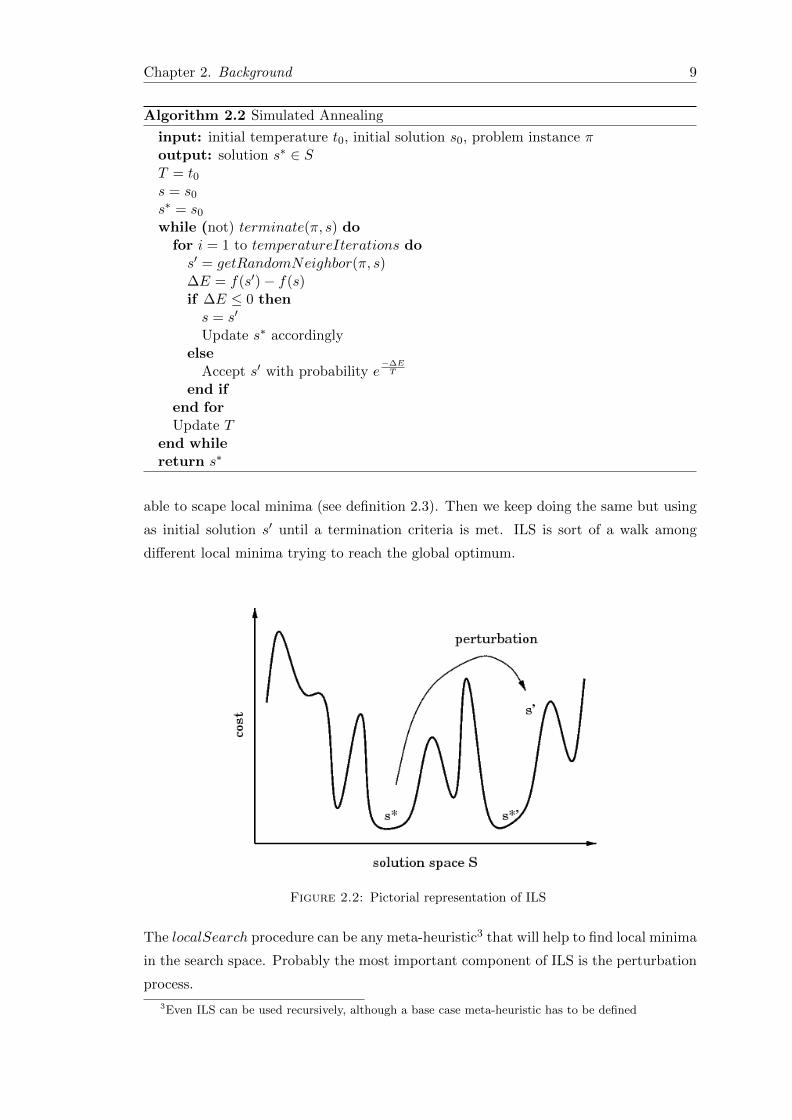
Chapter 2. Background 9
Algorithm 2.2 Simulated Annealing
input: initial temperature t0, initial solution s0, problem instance πoutput: solution s∗ ∈ ST = t0s = s0s∗ = s0while (not) terminate(π, s) do
for i = 1 to temperatureIterations dos′ = getRandomNeighbor(π, s)∆E = f(s′)− f(s)if ∆E ≤ 0 thens = s′
Update s∗ accordinglyelse
Accept s′ with probability e−∆E
T
end ifend forUpdate T
end whilereturn s∗
able to scape local minima (see definition 2.3). Then we keep doing the same but using
as initial solution s′ until a termination criteria is met. ILS is sort of a walk among
different local minima trying to reach the global optimum.
Figure 2.2: Pictorial representation of ILS
The localSearch procedure can be any meta-heuristic3 that will help to find local minima
in the search space. Probably the most important component of ILS is the perturbation
process.
3Even ILS can be used recursively, although a base case meta-heuristic has to be defined

Chapter 2. Background 10
Definition 2.6. A perturbation of a solution s is a series of modifications made to s
so that a new solution s1 is generated. Ideally this solution has to be different to s and
not be a member of the neighborhood of s, N(s).
The perturbation will help ILS to “jump” out of local minima and will start the local
search procedure, hopefully, in a unexplored part of the search space. It is easy to see
that the perturbation needs to have a random component to avoid falling into cycles
where the algorithm falls into the same local minima over and over again. The detailed
algorithm can be seen on Algorithm 2.3.
Algorithm 2.3 Iterated Local Search
s0 = GenerateInitialSolutions∗ = LocalSearch(s0)while termination condition not met dos′ = Perturbation(s∗)s∗′
= LocalSearch(s′)s∗ = AcceptanceCriterion(s∗, s∗
′)
end whilereturn s∗
The “AcceptanceCriterion” procedure on algorithm 2.3 refers to which of the solution
is going to be kept during each iteration. Usually just the best solution is taken into
account, but sometimes worse solutions can be accepted according to a probability func-
tion.
2.2 Meshes
According to Angel in [1] a mesh is “a set of polygons that share vertices and edges”.
An example of a mesh can be found on the model of a dolphin represented as a mesh
on Figure 2.3. In that context a vertex can be defined as a point in the 3D space of the
form (x, y, z) and an edge as a line segment connecting two vertices.
Usually a mesh is represented using only one kind of polygon to represent each part of
the mesh. Typically the basic polygon used is either a triangle or a quadrilateral. In
this text only triangular meshes will be used4 because of being always planar and convex
polygons.
Definition 2.7. A triangular mesh consists of the following elements:
• A set V of vertices in the 3D space where each vertex is a 3-tuple of the form
(x, y, z).
4Although it can easily be extended to any kind of polygons

Chapter 2. Background 11
Figure 2.3: Triangle mesh representing a dolphin
• A set F of triangle faces defined by a 3-tuple of vertices of the form (v1, v2, v3)
where each vi ∈ V and v1, v2 and v3 define the three vertices of the triangle in a
counter clockwise fashion.
• Optionally, a set Vn of vectors (3-tuples) defining the normal vector of each vertex
in V .
• Optionally, a set T of texture coordinates, for texture mapping enabled rendering.
2.3 Images
In computers, an image is seen as a matrix of colors. Each element of that matrix is
called a pixel. Depending on the resolution of the image there are less or more pixels
helping to define the image in more detail . For the purposes of this investigation, the
next definition of image will be used.
Definition 2.8. A pixel is 3-tuple (R,G,B) where each R,G and B represent the red,
blue and green components that makes a color.5
Definition 2.9. An image is a matrix (height × width) of pixels, where each pixel p
is associated with a position in the matrix (px, py).
2.3.1 Corner Detection on images
Image processing is a broad subject that has been thoroughly explored over the years.
Two important results from image processing are the algorithms used for edge detection
5The RGB color model is an additive color model in which red, green, and blue light are addedtogether in various ways to reproduce a broad array of colors.

Chapter 2. Background 12
and corner detection. According to Ritter et al. in [16] edge detection can be informally
defined as “a contour across which the brightness of the image changes abruptly in mag-
nitude or in the rate of change of magnitude”. In Figure 2.4 there is an example of how
the edges of an image look.
Figure 2.4: Applied edge detection
On the other hand a corner is a point where two or more edges meet. Those corners are
features in the image that help enormously to understand the structure inside the image,
making easier for specialized algorithms to identify what is represented in the image. In
Figure 2.5 there’s an example of an image with their respective corner detection.
Figure 2.5: Applied corner detection
“A successful tool is one that was
used to do something undreamt of by
its author.”
Stephen C. Johnson
Chapter 3
Tools
3.1 OpenCV
OpenCV1 is an open source framework focused on computer vision, which according to
Dradski et al.[3] is the transformation of data from a still or video camera into either a
decision or a new representation. All such transformations are done for achieving some
particular goal.
The project files can be obtained from the world wide web website http://SourceForge.
net/projects/opencvlibrary. The library is written in C and C++ and is multi
platform, being able to run under Linux, Windows and Mac OS X. There is a lot of
development on interfaces for Python, Ruby, Matlab, and other languages.
The main concern in the design of OpenCV was computational efficiency with a strong
focus on real time applications. The coding language used was optimized and it can
take advantage of multicore processors.
One of the main OpenCV’s goals is providing a simple to use infrastructure to develop
advanced vision applications in a short amount of time. It provides over 500 functions
that include many areas in vision, such as factory product inspection, medical imaging,
security, user interface, camera calibration, stereo vision, and robotics. It also provides
a comprehensive general-purpose Machine Learning Library (MLL) which is focused on
statistical pattern recognition and clustering.
OpenCV is used for the detection of corner in images given as an input that is going to
be matched against mesh vertices. See chapter 4 for more details.
1The Official OpenCV documentation can be found in [3]
13
Chapter 3. Tools 14
3.2 Wavefront (OBJ) Loader
We are using a program to import the meshes from OBJ files2 to C data structures
developed by Micah Taylor , a Computer Science graduate student from the University
of North Carolina at Chapel Hill.
The loader is written in C and includes a C++ wrapper. It can parse vertices, texture
4 coordinates, normals, 3 or 4 vertex faces, and .mtl files3. There is also support for
non-standard object types that are relevant to ray tracing. The code is freely distributed
and can be found at http://www.kixor.net/dev/objloader/ .
The OBJ format was used for loading the mesh information into the program developed
for testing the meta-heuristics so that the information could be easily accessed.
3.3 TAT Motion LabTM
TAT Motion Lab is an XML development environment for TAT Cascades4. It speeds
up the process of crafting rich user interfaces. Beside all the powerful editing features
TAT Motion Lab makes it possible to graphically manipulate visual productions.
The typical TAT Motion Lab user is more like a web programmer than visual designer.
TAT Motion Lab is a development environment that spans over the many aspects of TAT
Cascades, all the way from visual elements to XML model data. A comprehensive XML
editor has been introduced with automatic completion and validation of elements, tags
and attributes. In combination with comprehensive examples, templates and snippets
this creates a solid base from which you can build the next generation of user interfaces.
TAT Motion Lab works both as a prototyping environment and as an integrated produc-
tion environment with TAT Cascades. Combined, they enable designers and engineers
to create rich and astonishing multimedia user interfaces on any device, without losing
time or quality in the development process.
TAT Motion Lab was used for testing the transitions on a mobile device so that perfor-
mance would not be a problem.
2The Wavefront OBJ file specification can be found at [19]3The Material Template Library format (MTL) is a standard defined by Wavefront that complements
the OBJ file format. Its specification can be found at [18]4TAT Cascades is a UI framework for the production of advanced user interfaces, for more information
visit http://www.tat.se/site/products/cascades.html

Chapter 3. Tools 15
3.4 Blender
Blender5 is a 3D graphics application released as free software under the GNU General
Public License. It can be used for modeling, UV unwrapping, texturing, rigging, water
simulations, skinning, animating, rendering, particle and other simulations, non-linear
editing, compositing, and creating interactive 3D applications, including games.
Blender is available for a number of operating systems, including Linux, Mac OS X,
and Microsoft Windows. Blender’s features include advanced simulation tools such as
rigid body, fluid, cloth and soft-body dynamics, modifier-based modeling tools, powerful
character animation tools, a node-based material and compositing system and Python
for embedded scripting.
Blender was mainly used for the creation and edition of 3D models that were used for
testing the solution proposed.
5More information can be found at the web page http://www.blender.org/

“Problems are to the mind what
exercise is to the muscles, they
toughen and make strong”
Norman Vincent Peale
Chapter 4
Meta-heuristics design
The approach chosen to solve the study problem was to create a flat 3D mesh that
resembled as close as possible the 2D image provided as input and from which a smooth
transition to the final (given as input) 3D mesh could be performed. To create the
referred mesh, the corners of the 2D image are detected, then a proper match between
them and the input 3D mesh is done, and a flat mesh is created with strategically
placed vertices on the found corners positions. An example of a 2D image used, with
the corners detected highlighted is shown in Figure 4.1; and the corresponding mesh is
shown in Figure 4.2 .The way of doing the matching is important because the transition
of each vertex from the flat mesh to the final mesh is determined by it.
Figure 4.1: 2D input image that will be used in the problem with detected cornershighlighted
16
Chapter 4. Meta-heuristics design 17
Figure 4.2: 3D mesh corresponding to the the 2D image shown on Figure 4.1
4.1 Problem Description
The problem to be tackled on this investigation will be called from now on the Vertex
Assignment Problem. The formal definition is as follows:
Definition 4.1. The Vertex Assignment Problem (VAP) consists of finding an
optimal match between the corners of a given image and the vertices of a mesh. The
set of the image corners C has size |C| = n and the set of the mesh vertices V has size
|V | = m.
The match A is a m-tuple of the form (A1, A2, . . . , Am) where ∀i : 1 ≤ i ≤ m : Ai ∈ C.
Which means that the vertex vi is matched with the corner Ai.
Because there are nm possible matchings, the VAP is considered to be a NP problem 1.
Because of that meta-heuristical algorithms were chosen to solve the problem.
4.2 Goal Function
To be able to compare whether a matching A is better or worse than a matching B
a goal function has to be defined. For this problem the goal function was chosen to
represent non smooth transitions, that is, a high goal function value corresponds to a
1A simple transformation could be applied to convert the VAP into the QAP just by modifying thegoal function and neighbor structure in QAP

Chapter 4. Meta-heuristics design 18
coarse transition and a not very coherent vertex matching, whereas a small goal function
value corresponds to a coherent vertex matching and a smooth transition between the
2D image and the 3D mesh.
The factors considered in order to achieve a fair goal function are the following:
• The distance between vertices vi and vj (i, j ∈ [1,m]) should be as close as possible
to the distance between the matched corners Ai and Aj .
f1(s) =m∑i=1
m∑j=i+1
∣∣∣ d(Ai,Aj)2
MAXck,cl∈C{d(ck,cl)}2 −
d(vi,vj)2
MAXvk,vl∈V {d(vk,vl)}2
∣∣∣MAX
(d(Ai,Aj)
2
MAXck,cl∈C{d(ck,cl)}2 ,
d(vi,vj)2
MAXvk,vl∈V {d(vk,vl)}2
) (4.1)
where d(a, b) is the euclidean distance between points a and b. Each part of the
equation is explained next:
–∣∣∣ d(Ai,Aj)
2
MAXck,cl∈C{d(ck,cl)}2 −
d(vi,vj)2
MAXvk,vl∈V {d(vk,vl)}2
∣∣∣ represents the normalized differ-
ence between distances of vertices in the mesh minus their assigned corner.
This number is always between 0 and 1 since all distances have been normal-
ized, and the subtraction between them with always be in that interval.
– MAX(
d(Ai,Aj)2
MAXck,cl∈C{d(ck,cl)}2 ,
d(vi,vj)2
MAXvk,vl∈V {d(vk,vl)}2
)is the maximum value that
the numerator can have, thus normalizing each term of the inner sum to be
in the interval 0, 1.
With that preceding is easy to see that equation 4.1 can be at most m(m−1)2 .
• The distance between the transformation of the 2D image into a 3D model and the
original mesh is minimized. This tries to guarantee that the animation between
the mesh and the 3D representation of the image is as smooth as possible. This is
because the animation would be moving the vertices on the mesh to their respective
corners matched.
The transformation of the corners into the 3D space is going to be done using the
following points: a and a′ are points whose coordinates are the lowest in C and V
respectively and, d and d′ are points whose coordinates are the largest in C and
V respectively. Given that, any corner in C can be represented as a point in the
3D space by the next equation:

Chapter 4. Meta-heuristics design 19
g(x, y) = (
a′.x+x− a.xd.x− a.x
(d′.x− a′.x),
a′.y +y − a.yd.y − a.y
(d′.y − a′.y),
MINv∈V {v.z}
) (4.2)
With equation 4.2 a measurement of the distance between the mesh and the
matched corners can be written.
f2(s) =m∑i=1
d (vi, g (Ai.x, Ai.y))2
MAXAk∈A,vl∈V {d (g (Ak.x, Ak.y) , vl)}2(4.3)
Equation 4.3 calculates the minimum distance to be traveled in a transition be-
tween the matching mesh (applying equation 4.2 to the matching) against the
original mesh from the input. Since each term of the sum in equation 4.3 is at
most 1, then the equation is at most m.
With equations 4.1 and 4.3 a goal function can be described using different weights that
will allow further tuning to the goal function. The goal function f can be defined as:
f(s) =2ω1
m(m− 1)f1(s) +
ω2
mf2(s) (4.4)
where each wi ∈ R is the respective weight given to each part of the goal function
(∑wi = 1). The VAP consists of trying to find a matching that minimizes f .
4.3 Neighbor Operator
Given S as the space of all possible matchings then N : S → 2S is the neighbor function
defined as follows:
N(s) = {r ∈ S | all elements in r are equal to the elements in s except one} (4.5)
That neighbor function, for a matching s, gives all other matchings that one can get by
swapping an element si with a different corner cj ∈ C. The cardinality of N(s) (for a

Chapter 4. Meta-heuristics design 20
given matching s) is n(m− 1). Other neighbor operators were tried (e.g. changing more
than one vertex of the current solution), but they were not as effective or were more
time consuming than equation 4.5.
4.4 Initial Solution
As initial solution a semi-optimal solution is chosen in order to start the meta-heuristic
from a good enough solution in order to reduce the solution space exploration time. The
criteria used to choose this initial solution is the following:
Given a solution (matching) s, each si is assigned to the corner ck ∈ Cthat minimizes d (vi, g (ck.x, ck.y))
This semi-optimal criteria guarantees a fairly good start in the initial solution since the
vertex movements used to make possible animations between the 2D image and the 3D
meshes will be very few.
The initial solution chosen minimizes equation 4.3 by choosing always minimal values
for d (vi, g (ck.x, ck.y)). This achieves a very good start for the overall goal function on
equation 4.4.
4.5 Meta-heuristics implemented
All the meta-heuristics explained in Chapter 2 were implemented to solve the VAP.
4.5.1 Local Search: First improvement
With this approach a local search algorithm was used, but using as step function the
first neighbor found during the search through the neighbor structure that improved the
current solution on the algorithm.
4.5.2 Local Search: Best improvement
This approach also implements the local search meta-heuristic, but the step function
chooses the neighbor that improves the goal function the most across all the neighbor-
hood structure.

Chapter 4. Meta-heuristics design 21
4.5.3 Simulated annealing
In SA an approach similar to the one used for the QAP in [12] was used for the tem-
perature modification scheme. The temperature is updated according to the following
equation:
Ti+1 =Ti
1 + βTi(4.6)
where β is a factor dependent of the initial, final temperature (To and Tf respectively)
and total number of iterations to be run M .
β =To − TfMToTf
(4.7)
4.5.4 Iterated Local Search
The perturbation used by ILS was a simple appliance of the neighborhood operator
through the first 10 + m100 solutions found by the neighborhood operator. This pertur-
bation allows a fairly good separation from the initial solution, given more probability
to having escaped from local minima. The perturbation was tuned by experimentation
because of the experimental nature of the meta-heuristic.
A simple acceptance criteria was used, having at the end of each iteration the best
solution found until the moment. This criteria was chosen because after accepting worse
solutions on this problem would increase the difficulty of finding better solutions in the
long run.

“Insanity: doing the same thing over
and over again and expecting different
results.”
Albert Einstein
Chapter 5
Development and Results
5.1 Development
In order to test the meta-heuristics implemented a testing development framework had
to be used. The approach used was to match corners on images with vertices on 3D
meshes according to the pseudo-code presented in Algorithm 5.1. OpenCV is used in
the pre-processing step in order to get all the corners of the given image and to be able
to start doing the matching.
Algorithm 5.1 Framework used for testing
input: image img, mesh Moutput: graphical transition from img to MC = getImageCorners(img)s+ = applyMetaHeuristic(C,M)FM = transformMatchingToMesh(s+)graphicalTransition(FM,M)
The meshes used were in the OBJ format specification and the obj loader described in
Chapter 3 was used to load them into the memory.
5.2 Results
In Table 5.1 the results achieved by the meta-heuristics implemented are shown. The
test cases used are shown in more detail in Figures 5.1 and 5.5 for the Plane test-case;
in Figures 5.2 and 5.6 for the Cross; in Figures 5.3 and 5.7 for the Map test-case; and
in Figures 5.4 and 5.8 for the Dodecahedron test-case.
22

Chapter 5. Development and Results 23
LS: First LS: Best SA ILS Vertices
Plane 0.1371912 0.1371912 0.1371912 0.1371912 37451200.000s 1200.000s 126.045s 318.879s
Cross 0.1074486 0.1074478 0.1074486 0.1074478 242.733s 3.190s 1.417s 8.400s
Map 0.0649124 0.0649124 0.0649124 0.0649124 93641200.000s 1200.000s 668.739s 726.139s
Dodecahedron 0.3184613 0.3175088 0.3272882 0.3209643 2011.264s 8.045s 5.365s 5.102s
Table 5.1: Goal function results and times for the three test-cases tried
Figure 5.1: Plane input image used for running the Plane test-case
Figure 5.2: Cross input image used for running the Cross test-case
The best solutions found for the test-cases are shown in the Figures 5.9, 5.10, 5.11 and
5.12.All the results in Table 5.1 were produced using as goal function the equation 4.4
where the weights given to each part of the goal function were ω1 = 0.5 and ω2 = 0.5.
ω1 and ω2 were chosen both as 0.5 because then the goal function could give the same

Chapter 5. Development and Results 24
Figure 5.3: Map input image used for running the Map test-case
Figure 5.4: Dodecahedron input image used for the Dodecahedron test-case
importance both to structural matching and smooth transitions.
5.3 Discussion
In the three cases tested, a good overall match was achieved. This is in great part made
possible by the goal function defined and the election of the respective weights (ω1 = 0.5
and ω2 = 0.5). Without the contribution of ω2 to the goal function, good matchings
could be achieved (in a structural way) but sometimes the transition from the match to
the mesh was non smooth as observed in Figure 5.13.

Chapter 5. Development and Results 25
Figure 5.5: Plane input mesh used for the Plane test-case
Figure 5.6: Cross input mesh used for the Cross test-case
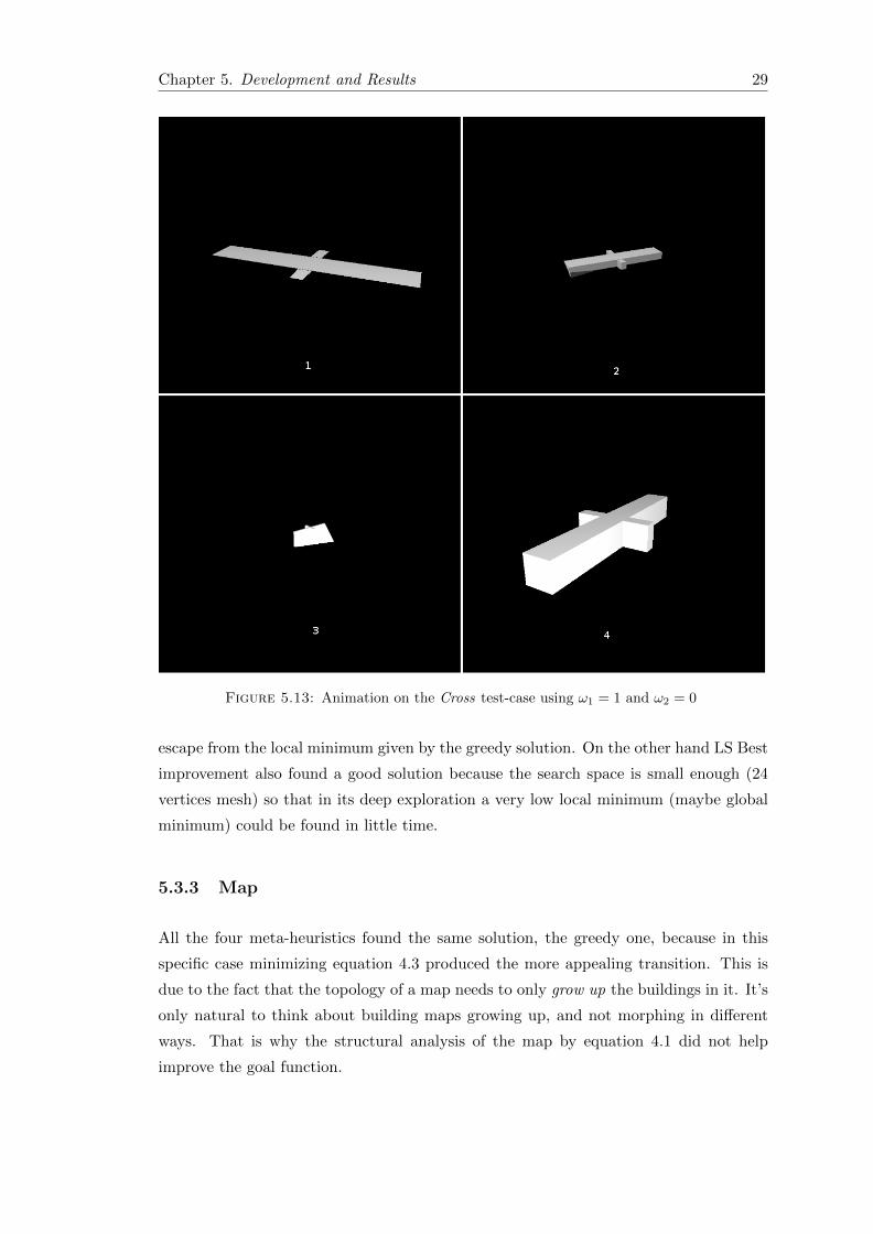
In the following subsections each test-case results will be analyzed so that a deeper
understanding of the problem could be obtained.
5.3.1 Plane
In Table 5.1 it can be seen that all algorithms found the same solution for this test-case.
This is due to the fact that the initial greedy solution minimizes equation 4.3 on the goal
Chapter 5. Development and Results 26
Figure 5.7: Map input mesh used for the Map test-case
Figure 5.8: Dodecahedron input mesh used for the Dodecahedron test-case
function, thereby making a very likely local minimum. That fact increases the difficulty
of finding a better match.
In the LS First Improvement and LS Best Improvement a timeout criteria was applied
after 20 minutes (1200s). The timeout was applied because the exhaustive nature of the
local search meta-heuristic explored in some occasions all the n(m−1) neighbors (about
127330 neighbors for each possible match in this case).

Chapter 5. Development and Results 27
Figure 5.9: Best Plane matching returned in the Plane test-case
Figure 5.10: Best Cross matching returned in the Cross test-case
5.3.2 Cross
In this test-case the greedy solution was not the best solution by any of the meta-
heuristics. The best matching was found both by ILS and LS Best improvement. This
best matching provided a really smooth transition because the growing of the mesh was
only in a vertical direction (as opposed to Figure 5.13).
In Figure 5.2 it can be noticed that for each geometric corner the corner detection
algorithm could detect both the inside and outside parts of the shape as they are also

Chapter 5. Development and Results 28
Figure 5.11: Best Map matching returned in the Map test-case
Figure 5.12: Best Dodecahedron matching returned in the Dodecahedron test-case
valid corners. The meta-heuristics were able to find a solution better than the greedy
because the structural part of the goal function (shown on equation 4.1) guaranteed
that all the corners were matched in a consistent way with the cross shape. That is the
angles between the corners were approximately right angles.
ILS could easily find that solution because of its perturbation model that allowed it to
Chapter 5. Development and Results 29
Figure 5.13: Animation on the Cross test-case using ω1 = 1 and ω2 = 0
escape from the local minimum given by the greedy solution. On the other hand LS Best
improvement also found a good solution because the search space is small enough (24
vertices mesh) so that in its deep exploration a very low local minimum (maybe global
minimum) could be found in little time.
5.3.3 Map
All the four meta-heuristics found the same solution, the greedy one, because in this
specific case minimizing equation 4.3 produced the more appealing transition. This is
due to the fact that the topology of a map needs to only grow up the buildings in it. It’s
only natural to think about building maps growing up, and not morphing in different
ways. That is why the structural analysis of the map by equation 4.1 did not help
improve the goal function.
Chapter 5. Development and Results 30
The local search meta-heuristics suffered from the same problem as in the Plane test-case
by running out of time because the Map has far more vertices than the Plane.
5.3.4 Dodecahedron
This test-case is very similar to the Cross test-case because it highlights a very symmetric
structure with several corners detected in the 2D image, which resulted in a non optimal
greedy solution that was improved by the meta-heuristics in all the cases as seen in Table
5.1.
LS-Best was the meta-heuristic that showed the best performance because it did a more
exhaustive search as it was a test-case where the whole neighborhood for each solution
could be easily explored.
5.3.5 Map Demo
At TAT, a map demo was developed to show some of the advantages of the transitions
between 2D and 3D. For this case, more visual effects were applied like texture mapping
and a manually done match between a map and a mesh to prove that the concept could
be further exploited. This shows the benefits of meta-heuristics for doing the matching,
since manual work is not needed with their use, making it possible to do the matching
in large scale projects. In Figure 5.14 the test-case is highlighted.

Chapter 5. Development and Results 31
Figure 5.14: Smooth transition between 2D and 3D maps

“If you are not willing to risk the
unusual, you will have to settle for the
ordinary.”
Jim Rohn
Chapter 6
Conclusion
Meta-heuristics have proved to be powerful tools for finding good solutions of hard
problems in a reasonable amount of time. The solution space shown by the problem
studied, presents goal functions with very irregular topology, i.e. neighbor solutions
tend to have abrupt differences between them, which increases the chances of getting
trapped in local minima.
Nevertheless, the meta-heuristics implemented proved to work well on traversing the
solution space in the search of optimal matchings, finding fairly good solutions in an
acceptable amount of time.
As seen in the results, the greedy initial solution produced good results in some instances
of the problem, giving a good start for the optimization procedure that in some cases
could not be beaten, as it represented a very good local minimum.
6.1 Recommendations for Future Research
This thesis was focused on solving the Vertex Assignment Problem described, through
the implementation and adaptation of the 2 known meta-heuristics: Simulated Annealing
and Iterated Local Search. The meta-heuristic algorithmic model is a broad and fast
growing subject in the Combinatorial Optimization field and there exists many different
meta-heuristics1 implementations with which this problem can be approached, such as:
Genetic Algorithms, Tabu Search, GRASP2, Ant Colony Optimization, among others.
Hybrid implementations of the named methods can also be tried, as they have proved
in many cases to work differently than the original unmerged ones.
1For detailed information about these meta-heuristics refer to [14]2Greedy Random Adaptive Search Procedure.
32

Chapter 6. Conclusion 33
Besides the meta-heuristics approach, different techniques can be tried as well, like
Constraint Programming[5] and Satisfiability Problem[11] (SAT) solving methods.
Bibliography
[1] Edward Angel. Interactive Computer Graphics, A Top-down Approach Using
OpenGL R©. Addison Wesley, 2009. ISBN 0321549430, 9780321549433.
[2] Christian Blum and Andrea Roli. Metaheuristics in combinatorial optimization:
Overview and conceptual comparison. ACM Comput. Surv., 35(3):268–308, 2003.
ISSN 0360-0300. doi: http://doi.acm.org/10.1145/937503.937505.
[3] Gary Dradski and Adrian Kaehler. Learning OpenCV. O’Reilly Media, Inc., 2008.
ISBN 9780596516130.
[4] Talbi El-Ghazali. Metaheuristics: From Design to Implementation. Wiley, New
Jersey, 2009.
[5] Peter van Beek Francesca Rossi and Toby Walsh. Handbook of Constraint Pro-
gramming (Foundations of Artificial Intelligence). Elsevier Science, 2006. ISBN
978-0444527264.
[6] Gregory Gutin and Abraham Punnen. The traveling salesman problem and its
variations. Springer, 2002. ISBN 1402006640, 9781402006647.
[7] Juris Hartmanis and American Mathematical Society. Computational complexity
theory. AMS Bookstore, 1989.
[8] Olivier Martin Helena Lorenco and Thomas Stutzle. Iterated local search. Handbook
of Metaheuristics, pages 321–353, 2003.
[9] Holger Hoos and Thomas St tzle. Stochastic Local Search. Morgan Kaufmann, 2004.
[10] P. Siarry J. Dreo, A. Petrowski and E. Taillard. Metaheuristics for Hard Optimiza-
tion. Springer, 2003.
[11] Panos M. Pardalos Jun Gu and Ding-Zhu Du. Satisfiability Problem: Theory
and Applications. American Mathematical Society, 1997. ISBN 0821804790,978-
0821804797.
34

Bibliography 35
[12] Per S. Laursen. Simulated annealing for the qap – optimal tradeoff between sim-
ulation time and solution quality. European Journal of Operational Research, 69
(2):238 – 243, 1993. ISSN 0377-2217. doi: DOI:10.1016/0377-2217(93)90167-L.
URL http://www.sciencedirect.com/science/article/B6VCT-48NBGX1-21M/
2/b899aa07c84af552f8f1fa9fc20a6a85.
[13] Eugene Lawler. The quadratic assignment problem. Management Science, 9(4):
586–599, 1963.
[14] Ibrahim H. Osman and James P. Kelly. Meta-heuristics: theory & applications.
Springer, 1996. ISBN 0792397002, 9780792397007.
[15] TAT Tenk Process. 3d user interfaces for mobile phones. Mobile User Experience
London, pages 1–25, 2008.
[16] Gerhard Ritter and Joseph Wilson. Handbook of Computer Vision Algorithms Im-
age Algebra. CRC Press, 2001.
[17] Luke Sean. Essentials of Metaheuristics. 2009. available at
http://cs.gmu.edu/∼sean/book/metaheuristics/.
[18] Wavefront Technologies. Material Template Library (.mtl). . available at
http://local.wasp.uwa.edu.au/∼pbourke/dataformats/mtl/.
[19] Wavefront Technologies. Object Files (.Obj). . available at
http://local.wasp.uwa.edu.au/∼pbourke/dataformats/obj/.
[20] Ronald Rivest Thomas Cormen, Charles Leiserson and Clifford Stein. Introduction
to algorithms. The MIT Press, 2001.
[21] Paolo Toth and Daniele Vigo. The vehicle routing problem. SIAM, 2002. ISBN
0898715792, 9780898715798.


![QAP Summary [R]](https://static.fdocuments.in/doc/165x107/577cc1221a28aba7119253d1/qap-summary-r.jpg)

