GENERATION INPUTS STUDY - BPA.gov - Bonneville ... Determining the Amount of Capacity Provided by...

B O N N E V I L L E P O W E R A D M I N I S T R A T I O N

2012 BPA Final Rate Proposal

Generation Inputs Study

July 2011

BP-12-FS-BPA-05

GENERATION INPUTS STUDY TABLE OF CONTENTS

Page

Commonly Used Acronyms and Short Forms .............................................................................. vii

1. INTRODUCTION ...............................................................................................................1 1.1 Purpose of Study ......................................................................................................1 1.2 Summary of Study ...................................................................................................1

2. BALANCING RESERVE CAPACITY QUANTITY FORECAST ...................................3 2.1 Introduction..............................................................................................................3

2.1.1 Purpose of the Balancing Reserve Capacity Quantity Forecast................3 2.1.2 Overview...................................................................................................3

2.2 Existing and Future Generation Projects for the Rate Period ..................................6 2.3 “Scaling in” Future Wind Generation......................................................................9

2.3.1 Methodology for Determining Lead and Lag Times ................................9 2.3.2 Estimating Future Wind Project Generation...........................................12

2.4 Accounting for Other Non-AGC Controlled Generation.......................................14 2.4.1 Analyzing Historical Use of Balancing Reserve Capacity .....................14 2.4.2 Accounting for Future Non-AGC Generation ........................................15 2.4.3 Accounting for Solar Generation ............................................................15

2.5 Load Estimates.......................................................................................................17 2.5.1 Accounting for Pump Load.....................................................................17 2.5.2 Actual Balancing Authority Area Load Amounts That

Correspond with Wind Penetration Levels .............................................18 2.5.3 Balancing Authority Area Load Forecasts..............................................18

2.6 Wind Scheduling Accuracy Assumption ...............................................................19 2.7 Balancing Reserve Capacity Requirements Methodology ....................................19

2.7.1 Base Methodology ..................................................................................19 2.7.2 Time Series of Studies ............................................................................21 2.7.3 Allocating the Total Balancing Reserve Capacity Requirement

Between Generation and Load................................................................23 2.7.4 Determining the Imbalance Reduction for Self-Supply..........................25

2.8 Committed Intra-Hour Scheduling Pilot................................................................26 2.9 Study of Quality of Service Levels in Excess of 99.5 Percent ..............................27 2.10 Results....................................................................................................................28

3. BALANCING RESERVE CAPACITY COST ALLOCATION METHODOLOGY ............................................................................................................31 3.1 Introduction............................................................................................................31 3.2 Embedded Cost Allocation Methodology..............................................................33

3.2.1 Description of the Portion of the FCRPS Used to Provide Balancing Reserve Capacity ...................................................................33

BP-12-FS-BPA-05 i

3.2.2 Determining the Amount of Capacity Provided by the FCRPS .............34 3.2.3 Source and Description of Inputs and Outputs of the HYDSIM

Model 35 3.2.4 Source and Description of HOSS and Modifications .............................36 3.2.5 120-Hour Federal System Hydro Capacity.............................................38 3.2.6 Detailed Development of 120-Hour Hydro Peaking Capacity ...............39 3.2.7 Big 10 Hydro 120-Hour Peaking Capacity for the Embedded

Cost Methodology...................................................................................39 3.2.8 Embedded Unit Cost Calculation............................................................40

3.3 Direct Assignment of Costs ...................................................................................43 3.3.1 WIT Costs ...............................................................................................43 3.3.2 Dec Acquisition Pilot Costs ....................................................................44

3.4 Variable Cost Pricing Methodology ......................................................................46 3.4.1 Introduction and Purpose ........................................................................46 3.4.2 Pre-processes and Inputs.........................................................................49 3.4.3 Stand Ready Costs ..................................................................................54 3.4.4 Deployment Costs...................................................................................59 3.4.5 Variable Cost of Reserves.......................................................................62

4. OPERATING RESERVE COST ALLOCATION ............................................................65 4.1 Introduction............................................................................................................65 4.2 Applicable Regional Reliability Standards for Operating Reserve .......................65 4.3 Calculating the Quantity of Operating Reserve Using the Current BAL-

STD-002-0 .............................................................................................................67 4.4 Calculating the Quantity of Operating Reserve Using the Proposed

Standard BAL-002-WECC-1.................................................................................68 4.5 Calculating the Operating Reserve Obligation Forecast........................................70 4.6 Cost Allocation for Operating Reserve..................................................................70

4.6.1 General Methodology for Pricing the Embedded Cost Portion of Operating Reserve...................................................................................70

4.6.2 Identify the System That Provides Operating Reserve ...........................71 4.6.3 Calculation of the Embedded Unit Cost of Operating Reserve

Capacity ..................................................................................................72 4.6.4 Forecast of Revenue from Embedded Cost Portion of Operating

Reserve....................................................................................................72 4.6.5 Total Cost Allocation and Unit Prices for Spinning Operating

Reserve....................................................................................................72

5. SYNCHRONOUS CONDENSING ..................................................................................75 5.1 Synchronous Condensing.......................................................................................75 5.2 Description of Synchronous Condensers ...............................................................75 5.3 Synchronous Condenser Costs...............................................................................75 5.4 General Methodology to Determine Energy Consumption ...................................76

5.4.1 Grand Coulee Project..............................................................................77 5.4.2 John Day, The Dalles, and Dworshak Projects.......................................78 5.4.3 Palisades Project .....................................................................................78 5.4.4 Willamette River Projects .......................................................................79

BP-12-FS-BPA-05 ii

5.4.5 Hungry Horse Project .............................................................................79 5.5 Summary – Costs Assigned to Transmission Services ..........................................79

6. GENERATION DROPPING.............................................................................................81 6.1 Introduction............................................................................................................81 6.2 Generation Dropping .............................................................................................81 6.3 Forecast Amount of Generation Dropping ............................................................81 6.4 General Methodology ............................................................................................82 6.5 Determining Costs to Allocate to Generation Dropping........................................82 6.6 Equipment Deterioration, Replacement, or Overhaul............................................83 6.7 Summary ................................................................................................................84

7. REDISPATCH...................................................................................................................85 7.1 Introduction............................................................................................................85 7.2 Discretionary Redispatch .......................................................................................86 7.3 NT Redispatch .......................................................................................................86 7.4 Emergency Redispatch...........................................................................................87 7.5 Revenue Forecast for Attachment M Redispatch Service .....................................88

8. SEGMENTATION OF CORPS OF ENGINEERS AND BUREAU OF RECLAMATION TRANSMISSION FACILITIES .........................................................89 8.1 Introduction............................................................................................................89 8.2 Generation Integration ...........................................................................................89 8.3 Integrated Network ................................................................................................90 8.4 Utility Delivery ......................................................................................................90 8.5 COE Facilities........................................................................................................90 8.6 Reclamation Facilities............................................................................................90

8.6.1 Columbia Basin Transmission Costs ......................................................91 8.7 Revenue Requirement for Investment in COE and Reclamation Facilities...........92

9. STATION SERVICE.........................................................................................................95 9.1 Introduction............................................................................................................95 9.2 Overview of Methodology.....................................................................................95 9.3 Assessment of Installed Transformation................................................................96 9.4 Assessment of Station Service Energy Usage .......................................................96 9.5 Calculation of Average Load Factor......................................................................96 9.6 Calculating the Total Quantity of Station Service .................................................97 9.7 Determining Costs to Allocate to Station Service .................................................97 9.8 Impact on Power Rates and Transmission Rates ...................................................97

10. ANCILLARY AND CONTROL AREA SERVICES .......................................................99 10.1 Introduction............................................................................................................99 10.2 Ancillary Services and Control Area Services.......................................................99

10.2.1 Ancillary Services...................................................................................99 10.2.2 Control Area Services ...........................................................................100 10.2.3 Ancillary Services and Control Area Services Rate Schedules ............101

10.3 Regulation and Frequency Response Service Rate..............................................101

BP-12-FS-BPA-05 iii

10.3.1 RFR Sales Forecast ...............................................................................102 10.3.2 RFR Rate Calculation ...........................................................................102

10.4 Operating Reserve Service Rates.........................................................................103 10.4.1 Spinning Reserve Service .....................................................................104 10.4.2 Supplemental Reserve Service..............................................................105 10.4.3 Operating Reserve Rate Calculation.....................................................106

10.5 VERBS.................................................................................................................107 10.5.1 VERBS Rate Calculation......................................................................108 10.5.2 Formula Rate I: Rate Adjustment for Replacement of Federal

Generation Inputs for VERBS ..............................................................110 10.5.3 Formula Rate II: Rate Adjustment to Increase Generation Inputs

for VERBS............................................................................................112 10.5.4 Provisional VERBS (Provisional Balancing Service) ..........................113

10.6 Dispatchable Energy Resource Balancing Service (DERBS) .............................115 10.6.1 Rate Calculation....................................................................................115

10.7 Energy Imbalance and Generation Imbalance Service ........................................117 10.7.1 Energy Imbalance Service ....................................................................118 10.7.2 Generation Imbalance Service ..............................................................119

10.8 Persistent Deviation for Imbalance Services .......................................................121 10.8.1 Introduction...........................................................................................121 10.8.2 Study Summary.....................................................................................121 10.8.3 Definition of Persistent Deviation for the FY 2010–2011 Rate

Period 121 10.8.4 Definitions of Relevant Terms..............................................................124 10.8.5 Persistent Deviations During FY 2010 .................................................125 10.8.6 Operational Impacts of Persistent Deviations.......................................128 10.8.7 Comparison of 30-Minute Persistence Scheduling to Observed

Actual Wind Generation Scheduling ....................................................130 10.8.8 Examples of Schedule Errors That Result in Imbalance

Accumulation But Are Not Captured by the FY 2010–2011 Definition of Persistent Deviation ........................................................133

10.8.9 Additional Refinements and Criteria for Persistent Deviation .............136 10.8.10 Persistent Deviation Penalty and Definition .........................................141

BP-12-FS-BPA-05 iv

TABLES Table 1 Power Services' Generation Inputs Revenue Forecast for FY 2012–2013 99.5%

Level of Service with Customer-Supplied Generation Imbalance..............................142 Table 2 Cost Allocation of VERBS Components for 99.5% Level of Service with

Customer-Supplied Generation Imbalance .................................................................143 Table 3 Calculation of Ancillary and Control Area Service Rates Variable Energy

Resource Balancing Service, Dispatchable Energy Resource Balancing Service, Regulation and Frequency Response, and Operating Reserve......................144

FIGURES Figure 1: Trends in Percentage of Hours Meeting 20MW/15 percent/4hr Criteria....................127 Figure 2: Accumulation of Imbalance Energy (MWh)...............................................................130 Figure 3: Rolling 24-Hour Accumulated Imbalance From 30-Minute Persistence

Scheduling for the BPA Wind Fleet............................................................................132 Figure 4: Rolling 24-Hour Accumulated Imbalance From the BPA Wind Fleet .......................132 Figure 5: Persistent Underscheduling .........................................................................................134 Figure 6: Zig-Zag Scheduling.....................................................................................................135 Figure 7: Diurnal Pattern ............................................................................................................136

BP-12-FS-BPA-05 v

This page intentionally left blank.

BP-12-FS-BPA-05 vi

COMMONLY USED ACRONYMS AND SHORT FORMS AGC Automatic Generation Control ALF Agency Load Forecast (computer model) aMW average megawatt(s) AMNR Accumulated Modified Net Revenues ANR Accumulated Net Revenues ASC Average System Cost BiOp Biological Opinion BPA Bonneville Power Administration Btu British thermal unit CDD cooling degree day(s) CDQ Contract Demand Quantity CGS Columbia Generating Station CHWM Contract High Water Mark Commission Federal Energy Regulatory Commission COSA Cost of Service Analysis COU consumer-owned utility Corps or USACE U.S. Army Corps of Engineers Council Northwest Power and Conservation Council CRAC Cost Recovery Adjustment Clause CSP Customer System Peak CT combustion turbine CY calendar year (January through December) DDC Dividend Distribution Clause dec decrease, decrement, or decremental DERBS Dispatchable Energy Resource Balancing Service DFS Diurnal Flattening Service DOE Department of Energy DSI direct-service industrial customer or direct-service industry DSO Dispatcher Standing Order EIA Energy Information Administration EIS Environmental Impact Statement EN Energy Northwest, Inc. EPP Environmentally Preferred Power ESA Endangered Species Act e-Tag electronic interchange transaction information FBS Federal base system FCRPS Federal Columbia River Power System FCRTS Federal Columbia River Transmission System FELCC firm energy load carrying capability FORS Forced Outage Reserve Service FPS Firm Power Products and Services (rate) FY fiscal year (October through September) GARD Generation and Reserves Dispatch (computer model) GEP Green Energy Premium

BP-12-FS-BPA-05 vii

GRSPs General Rate Schedule Provisions GTA General Transfer Agreement GWh gigawatthour HDD heating degree day(s) HLH Heavy Load Hour(s) HOSS Hourly Operating and Scheduling Simulator (computer model) HYDSIM Hydro Simulation (computer model) ICE IntercontinentalExchange inc increase, increment, or incremental IOU investor-owned utility IP Industrial Firm Power (rate) IPR Integrated Program Review IRD Irrigation Rate Discount JOE Joint Operating Entity kW kilowatt (1000 watts) kWh kilowatthour LDD Low Density Discount LLH Light Load Hour(s) LRA Load Reduction Agreement Maf million acre-feet Mid-C Mid-Columbia MMBtu million British thermal units MNR Modified Net Revenues MRNR Minimum Required Net Revenue MW megawatt (1 million watts) MWh megawatthour NEPA National Environmental Policy Act NERC North American Electric Reliability Corporation NFB National Marine Fisheries Service (NMFS) Federal Columbia

River Power System (FCRPS) Biological Opinion (BiOp) NLSL New Large Single Load NMFS National Marine Fisheries Service NOAA Fisheries National Oceanographic and Atmospheric Administration

Fisheries NORM Non-Operating Risk Model (computer model) Northwest Power Act Pacific Northwest Electric Power Planning and Conservation

Act NPV net present value NR New Resource Firm Power (rate) NT Network Transmission NTSA Non-Treaty Storage Agreement NUG non-utility generation NWPP Northwest Power Pool OATT Open Access Transmission Tariff O&M operation and maintenance OMB Office of Management and Budget

BP-12-FS-BPA-05 viii

OY operating year (August through July) PF Priority Firm Power (rate) PFp Priority Firm Public (rate) PFx Priority Firm Exchange (rate) PNCA Pacific Northwest Coordination Agreement PNRR Planned Net Revenues for Risk PNW Pacific Northwest POD Point of Delivery POI Point of Integration or Point of Interconnection POM Point of Metering POR Point of Receipt Project Act Bonneville Project Act PRS Power Rates Study PS BPA Power Services PSW Pacific Southwest PTP Point to Point Transmission (rate) PUD public or people’s utility district RAM Rate Analysis Model (computer model) RAS Remedial Action Scheme RD Regional Dialogue REC Renewable Energy Certificate Reclamation or USBR U.S. Bureau of Reclamation REP Residential Exchange Program RevSim Revenue Simulation Model (component of RiskMod) RFA Revenue Forecast Application (database) RHWM Rate Period High Water Mark RiskMod Risk Analysis Model (computer model) RiskSim Risk Simulation Model (component of RiskMod) ROD Record of Decision RPSA Residential Purchase and Sale Agreement RR Resource Replacement (rate) RSS Resource Support Services RT1SC RHWM Tier 1 System Capability RTO Regional Transmission Operator SCADA Supervisory Control and Data Acquisition SCS Secondary Crediting Service Slice Slice of the System (product) T1SFCO Tier 1 System Firm Critical Output TCMS Transmission Curtailment Management Service TOCA Tier 1 Cost Allocator TPP Treasury Payment Probability Transmission System Act Federal Columbia River Transmission System Act TRL Total Retail Load TRM Tiered Rate Methodology TS BPA Transmission Services TSS Transmission Scheduling Service

BP-12-FS-BPA-05 ix

BP-12-FS-BPA-05 x

UAI Unauthorized Increase ULS Unanticipated Load Service USACE or Corps U.S. Army Corps of Engineers USBR or Reclamation U.S. Bureau of Reclamation USFWS U.S. Fish and Wildlife Service VERBS Variable Energy Resources Balancing Service (rate) VOR Value of Reserves WECC Western Electricity Coordinating Council (formerly WSCC) WIT Wind Integration Team WSPP Western Systems Power Pool

1. INTRODUCTION 1

2

3

4

5

6

7

8

9

11

12

13

14

15

16

17

18

19

20

22

23

24

25

The Federal Columbia River Power System (FCRPS) hydroelectric projects support BPA’s

transmission system and are instrumental in maintaining its reliability. In the context of this

Generation Inputs Study (Study), FCRPS is used to refer to only generation assets. For

ratesetting purposes, these uses of the FCRPS are quantified and the costs associated with these

uses are allocated to transmission rates under the ratesetting principle of cost causation. The uses

of the FCRPS to support the transmission system and maintain reliability are generally referred

to as generation inputs.

1.1 Purpose of Study 10

The Study explains the various cost allocations for generation inputs, forecasts revenues

associated with provision of these generation inputs, and describes the methodology used to set

the Ancillary and Control Area Services rates that recover the generation input costs. The

revenues that are forecast in the Study are applied in ratesetting as revenue credits in the Power

Rates Study, BP-12-FS-BPA-01, section 4. Generation inputs include energy and balancing

reserve capacity from the FCRPS that BPA uses to provide Ancillary and Control Area Services

and to maintain reliability of the transmission system. The Ancillary and Control Area Services

rates that are described in the Study are shown in the Transmission, Ancillary and Control Area

Service Rate Schedules, BP-12-A-02C.

1.2 Summary of Study 21

BPA provides balancing reserve capacity generation inputs for: Regulating Reserve, Following

Reserve, Variable Energy Resource Balancing Service (VERBS) Reserve, and Dispatchable

Energy Resource Balancing Service (DERBS) Reserve. The methodology for deriving the

forecast amount of balancing reserve capacity needed to provide these services is described in

BP-12-FS-BPA-05 Page 1

section 2 of the Study. The cost allocation methodology for these services is described in

section 3 of the Study. Section 4 of the Study addresses Operating Reserve (Contingency

Reserve) and details the methodology for determining the forecast need and cost allocation for

the Operating Reserve services. Other generation inputs, including Synchronous Condensing,

Generation Dropping, Redispatch Service, and Station Service are discussed in sections 5

through 9. Section 10 of the Study contains the description of the rate design for the Ancillary

and Control Area Service rates associated with generation inputs.

1

2

3

4

5

6

7

8

9

10

11

12

13

14

15

16

17

18

19

20

21

22

23

24

25

26

A summary of the revenue forecast for supplying these generation inputs is shown in Table 1 of

the Study. Table 1 shows the annual average revenue forecast for each generation input for the

rate period, including separate lines for embedded cost, variable cost, and where applicable,

direct assignment cost revenues. For most of the generation inputs Table 1 provides the

applicable quantities. Also, Table 1 shows an embedded unit cost for Regulating Reserve,

VERBS Reserve, DERBS Reserve, and Operating Reserve. These unit costs are used to

determine the forecast annual average revenue and should not be confused with the Ancillary and

Control Area Service rates for these services. The calculation and assumptions for each line in

Table 1 are explained in detail in the applicable sections of the Study. The Ancillary and Control

Area Service rates are shown in Table 3.

The VERBS rate contains three components, regulation, following, and imbalance. Costs

assigned to the VERBS are allocated to these three components and these costs are shown in

Table 2. The three components are used to calculate the VERBS rate. Table 3. The VERBS rate

is based on a 99.5 level of service described in section 2. As explained in section 10, the

Administrator retains the discretion under certain circumstances to increase the level of service

for the VERBS above 99.5 percent and adopt a higher rate during the rate period.


2. BALANCING RESERVE CAPACITY QUANTITY FORECAST 1

4

5

6

7

8

9

10

11

12

13

14

16

17

18

19

20

21

22

23

24

2.1 Introduction 2

2.1.1 Purpose of the Balancing Reserve Capacity Quantity Forecast 3

The Balancing Reserve Capacity Quantity Forecast estimates the amount of balancing reserve

capacity needed for BPA to provide certain Ancillary and Control Area Services during the rate

period. The forecast described in this section focuses on the balancing reserve capacity needed

to provide regulating reserves, following reserves, and imbalance reserves – collectively called

balancing services. The quantity of balancing reserve capacity that is forecast for each service is

an essential input for the cost allocation methodology used to establish the rates for these

services and the revenue credit associated with providing the balancing reserve capacity. See

sections 3 and 10 of this Study. In addition, the Balancing Reserve Capacity Quantity Forecast is

used to define the amount of balancing reserve capacity that BPA will make available for

purposes of operational limits imposed under Dispatcher Standing Order 216 (DSO 216).

2.1.2 Overview 15

As a Balancing Authority, BPA must maintain load-resource balance in its Balancing Authority

Area at all times. All generators within the BPA Balancing Authority Area provide hourly

generation schedules to BPA that estimate the average amount of energy they expect to generate

in the coming hour. Based on these schedules, BPA identifies an estimate of the average amount

of load to be served in the BPA Balancing Authority Area in the coming hour.

Transmission customers submit hourly transmission schedules, identifying all energy to be

transmitted across or within the BPA Balancing Authority Area in the coming hour. BPA uses

the transmission schedules to match generation inside the BPA Balancing Authority Area and


imports of energy from other balancing authority areas with loads served inside the BPA

Balancing Authority Area and exports to other balancing authority areas. The transmission

schedules identified with each adjacent balancing authority area are netted to determine

interchange schedules. The interchange schedules are netted for the BPA Balancing Authority

Area to determine controller totals.

1

2

3

4

5

6

7

8

9

10

11

12

13

14

15

16

17

18

19

20

21

22

23

24

25

26

Controller totals are the sum of all energy transactions to and from the BPA Balancing Authority

Area. Controller totals are used in the BPA Automatic Generation Control (AGC) system to

calculate the deviation between the actual interchange flows and the controller totals plus

dynamic schedules that affect the controller total amount. The AGC system regulates the output

of some specified Federal Columbia River Power System (FCRPS) generators in the BPA

Balancing Authority Area in response to changes in load, system frequency, and other factors to

maintain the scheduled system frequency and interchanges with other balancing authority areas.

The interchange schedules and controller totals do not change when a generator deviates from its

scheduled generation or loads deviate from the average hourly estimate, and the Balancing

Authority Area must use its own generation resources connected to the AGC system to offset

differences between scheduled and actual generation and to maintain within-hour load-resource

balance in the Balancing Authority Area.

BPA’s AGC system adjusts the generation of plants on automatic control based on the

differences between scheduled and actual load and generation. If load increases, or generation

decreases, the AGC system increases (incs) FCRPS generation. If load decreases, or generation

increases, the AGC system decreases (decs) FCRPS generation. The cumulative inc and dec

generation required to maintain load-resource balance within the hour forms the basis for the

balancing reserve capacity that BPA must have to provide balancing services.


Specific FCRPS generating resources under AGC control are designated by BPA to provide the

generation inputs necessary to supply balancing services. Utilizing the FCRPS resources to

provide generation inputs for balancing services affects the hydraulic operation of those facilities

and limits the availability of water for other uses. The FCRPS will use water to generate

additional power to replace generation from a resource within the Balancing Authority Area that

generates below its schedule or to serve a load that takes more energy than its schedule.

Conversely, BPA will store water and/or withhold capacity (both hydraulic capacity in the form

of reservoir space and turbine capacity) from other uses to adjust for a resource in the Balancing

Authority Area that generates above its schedule or loads that perform below their schedules.

1

2

3

4

5

6

7

8

9

10

11

12

13

14

15

16

17

18

19

20

21

22

23

24

25

26

27

BPA’s balancing reserve capacity requirements consists of three components: regulating

reserve, following reserve, and imbalance reserve. Regulating reserve refers to the capacity

necessary to provide for the continuous balancing of resources (generation and interchange) with

load on a moment-to-moment basis.

Following reserve generally refers to spinning and non-spinning capacity to meet within-hour

shifts of average energy due to variations of actual load and generation from forecast load and

generation. The Balancing Reserve Capacity Quantity Forecast estimates the balancing reserve

capacity needed to follow these average energy shifts according to a ten-minute clock cycle.

The imbalance reserve component refers to the impact on the following reserve amount due to

the difference (i.e., imbalance) between the average scheduled energy over the hour and the

average actual energy over the hour. Taking imbalance into account when calculating the

following reserve increases the following reserve amount due to the impact associated with

assuming the error from imperfect scheduling prior to the hour. Imbalance does not affect the

requirements for the regulating reserve component. The Balancing Reserve Capacity Quantity

Forecast estimates the incremental amount of following reserve that must be set aside for


imbalance and defines this amount as the imbalance reserve capacity component of the balancing

reserve capacity requirements.

1

2

3

4

5

6

7

8

9

10

11

12

13

14

15

17

18

19

20

21

22

23

24

25

The Balancing Reserve Capacity Quantity Forecast methodology is based primarily on (1) a

forecast of wind, solar, hydroelectric, and thermal facilities expected to come online during the

rate period; (2) total non-Federal thermal generation and scheduling data for the BPA Balancing

Authority Area from October 2009 to April 2010 and October 2010 to April 2011, and (3) data

from a 24-month period from October 1, 2007, to September 30, 2009. The data from the

24-month period needed for the forecast includes the total wind generation, the total

hydroelectric generation, the total hydroelectric schedule, the total Federal thermal generation,

the total Federal thermal schedule, the total non-Federal thermal generation, the total non-Federal

thermal schedule, the Balancing Authority Area load, and the Balancing Authority Area load

forecast for the period. Sections 2.2 through 2.6 describe in detail how the forecast methodology

data were obtained or developed.

2.2 Existing and Future Generation Projects for the Rate Period 16

Developing the Balancing Reserve Capacity Quantity Forecast required to provide balancing

services during the rate period requires an estimate of the amount of generation that will be

online during that period. This estimate includes both the actual generating facilities that are

online as of the time of the Study based on BPA records (see

http://transmission.bpa.gov/Business/Operations/Wind/WIND_InstalledCapacity_current.xls)

and a forecast of the facilities that are expected to come online before or during the FY 2012–

2013 rate period. See Generation Inputs Study Documentation, BP-12-FS-BPA-05A

(Documentation), Tables 2.1, 2.2, and 2.3.


The forecast of facilities that are expected to come online before or during the FY 2012–2013

rate period is based on a review of the pending requests in BPA’s generator interconnection

queue, information provided for the requests under BPA’s Large Generator Interconnection

Procedures (LGIP), and the application of certain criteria. The majority of new generating

facilities that are expected to come online prior to or during the rate period are wind facilities;

therefore, the estimates about future facilities pertain primarily to wind generation. References

to “future” or “planned” facilities throughout this Study indicate expectations with respect to the

interconnection of certain generating facilities based on the assessment of the circumstances and

information available at the time but are not intended to convey certainty about interconnection

of a particular generating facility.

1

2

3

4

5

6

7

8

9

10

11

12

13

14

15

16

17

18

19

20

21

22

23

24

25

26

27

To forecast which future generating facilities will interconnect and the timing of such

interconnections, BPA considers balancing service elections submitted by generators and the

status of interconnection requests in BPA’s interconnection queue in May 2011. For the

evaluation of the interconnection queue, the requested interconnection date in each

interconnection request is only one of several factors considered to assess a potential

interconnection date for a project. Prior to interconnecting, each future project must go through

the LGIP study process, under which BPA completes a series of studies prior to offering an

interconnection agreement and interconnection date. This can be an extended process, and the

timing for the completion can vary substantially; therefore, the evaluation of certain objective

factors is necessary to make projections about the status of future projects. Some of the factors

include:

1. The status of the interconnection study process. Requests in the earlier stages of

the study process are less likely to interconnect in the near term and are more

likely to be delayed past the requested online date.

2. The status of the environmental review process and interconnection customer

permitting process for the request. As a Federal agency, BPA must conduct a


review under the National Environmental Policy Act (NEPA) and other Federal

laws before deciding whether to interconnect a particular generator. This review

can take a substantial amount of time, and BPA typically coordinates its review to

coincide with the customer’s state or county environmental permitting process.

Requests that are not far along in those processes are less likely to interconnect in

the near term.

1

2

3

4

5

6

7

8

9

10

11

12

13

14

15

16

17

18

19

20

21

22

23

24

25

26

27

3. Interconnection and network facility additions that affect the time required to

complete an interconnection. As studies progress, BPA and the customer develop

a more definite plan of service, and the time to construct is better defined. The

particular network additions and interconnection facilities required to interconnect

the generator and the time it would take to construct those facilities are taken into

account.

4. Information received in direct discussions with each developer about its plans

(project scheduling, financing, turbine ordering commitment). A significant

factor that affects the interconnection forecast is the date when a customer

executes an engineering and procurement agreement, which allows BPA to

incorporate the project in BPA’s construction program schedule, begin work on

the necessary interconnection facilities design, and begin ordering materials and

equipment with a long procurement lead time.

5. The execution of an interconnection agreement and commitment by the customer

to fund all BPA facilities necessary for the interconnection. A firm construction

program schedule is included in the agreement. Executing an interconnection

agreement usually occurs just prior to the construction phase of a project.

Documentation, Table 2.1 identifies the amount of installed capacity that the Study assumes will

be online during the FY 2012–2013 rate period for each type of generation accounted for in the

Balancing Reserve Capacity Quantity Forecast. The forecast of installed wind capacity is an


average of 4,693 MW; installed solar capacity is an average of 21 MW; non-AGC controlled

hydroelectric capacity is an average of 2,604 MW; non-Federal thermal capacity is an average of

5,784 MW; and Federal thermal capacity is 1,276 MW.

1

2

3

4

7

8

9

10

11

12

13

14

15

16

17

18

19

20

21

22

23

24

25

26

2.3 “Scaling in” Future Wind Generation 5

2.3.1 Methodology for Determining Lead and Lag Times 6

Forecasting the balancing requirements for future wind generation during the rate period requires

estimating future minute-by-minute generation levels of all existing and future wind facilities in

the BPA Balancing Authority Area. For data on generation of the existing wind facilities,

24 months of one-minute actual average generation data from BPA’s Plant Information (PI)

system is used. The data cover generation from all existing wind generators in the BPA

Balancing Authority Area for the period from October 1, 2007, to September 30, 2009. For wind

facilities that came online between October 1, 2007, and September 30, 2009, a combination of

estimated minute-by-minute generation levels (prior to their online date) and one-minute actual

average generation data from BPA’s PI system (after their online date) is used. For wind

facilities online or forecast to come online after September 30, 2009, only estimated minute-by-

minute generation levels are used.

To help estimate minute-by-minute generation for future facilities and to aid in data scrubbing

for larger sections (greater than 20 minutes) of existing generator data, the time delays between

existing wind projects in BPA’s Balancing Authority Area and the locations of future and

existing wind projects are used. Documentation, Table 2.2 includes a map that shows the

locations of the wind projects in the Balancing Reserve Capacity Quantity Forecast for the

FY 2012–2013 rate period. A west-to-east wind pattern prevails generally in the locations of

many future and existing wind projects in BPA’s Balancing Authority Area, and future wind

project generation is assumed to be predicted generally by using leading (earlier in time)


generation values from an existing project that is west of the future project or lagging (later in

time) values from an existing project that is east of the future project.

1

2

3

4

5

6

7

8

9

10

11

12

13

14

15

16

17

18

19

20

21

22

23

24

25

26

The study determines the time delays in different ways depending on the data available for

particular projects. For existing projects online prior to January 1, 2011, BPA derived time

delays using actual minute-by-minute generation data from BPA’s PI system. To derive time

delays from the actual minute-by-minute data, a mathematical modeling tool, MATLAB, was

used to calculate correlations between the minute-by-minute data for all existing wind projects at

different time offsets. The time offsets used for this analysis were up to 240 minutes leading and

up to 240 minutes lagging. For each pair of existing and future wind projects, the time delay

resulting in the highest correlation was used to define the time delay between those projects.

For projects that were not online prior to January 1, 2011, the Study uses either data reflecting

common delays between existing projects and future project locations that were used in the

FY 2010–2011 rate case or time delays derived from numerical weather prediction model data.

BPA obtained both the data regarding the common time delays used in the FY 2010–2011 rate

case and the numerical weather prediction model data from 3TIER, a wind forecasting company

in Seattle, Washington. The time-delay data include a number of zero-minute values that

indicate minimal or no difference (lead or lag) in the ramp up or down time between particular

facilities or locations, but observations based on existing wind facilities indicate that wind

facilities seldom ramp up or down at exactly the same time. As a result, if the most prevalent

lead or lag time in the 3TIER data reflecting the common delays is zero minutes, the data are

adjusted to reflect a lead or lag based on BPA Staff observations and knowledge of the area in

question. With this adjustment, zero value leads or lags are minimized in the data used to scale

in the future wind facilities.


For projects that were not included in the 3TIER time-delay study for the FY 2010–2011 rate

case, time delays were calculated using the numerical weather prediction model data provided by

3TIER, which predicted wind speed at standard gridded locations across the Pacific Northwest

for calendar year (CY) 2004-2006 at ten-minute intervals. Using the forecast of wind generation

described in section 2.2 and its associated geographic coordinates (latitude and longitude), ten-

minute interval time series data were extracted for all existing and future wind projects. To

derive time delays from the numerical weather prediction model data, MATLAB was used to

calculate correlations between the ten-minute interval time series data for all existing and future

wind projects at different time offsets. The time offsets used for this analysis were up to 240

minutes leading and up to 240 minutes lagging. For each pair of existing and future wind

projects, the time delay resulting in the highest correlation was used to define the time delay

between those projects. These time delays also resulted in a number of zero-minute values that

indicate minimal or no difference (lead or lag) in the ramp up or down time between particular

facilities or locations. As a result, if the most prevalent lead or lag time in the 3TIER data

reflecting the common delays is zero minutes, the data were adjusted to reflect a lead or lag

based on Staff’s observations and knowledge of the area in question. With this adjustment, zero-

value leads or lags are minimized in the data used to scale in the future wind facilities.

1

2

3

4

5

6

7

8

9

10

11

12

13

14

15

16

17

18

19

20

21

22

23

24

25

26

27

In analyzing the lead or lag between a specific future project and an existing project, data for

more than one existing project are used. Using multiple existing projects helps to reflect some of

the “diversity” or operational variability that occurs between particular projects. In addition, all

generation data obtained from BPA’s PI system are reviewed for missing data. Any missing data

points that are less than or equal to 20 continuous sections (minutes) are filled in using linear

interpolation from the existing data and by manually filling in certain points (particularly for

values that are near zero). Any sections of missing data points larger than 20 minutes are filled

in using the scaling method used to estimate minute-by-minute generation for future facilities.

This method helps ensure that the filled-in data reflect the trends of BPA’s PI system data.


Documentation, Table 2.3 identifies the existing and future wind facilities that are forecast to be

online during the rate period. The table is organized according to the month and year that the

facility went into service or is expected to be in service. Entries for existing facilities include the

installed capacity in megawatts and the month and year that the facility reached its installed

capacity. Entries for the future wind projects include the installed capacity and the completion

date (month and year) on which the project is expected to reach its installed capacity. The

information in columns D through F titled “Reference Plant [1, 2, or 3]” identifies the facilities

used to scale the generation of a particular facility. Columns J through L titled “Reference Plant

[1, 2, or 3] Time Offset (minutes)” includes the lead and/or lag times in minutes from the

relevant reference plant to the facility being scaled.

1

2

3

4

5

6

7

8

9

10

11

13

14

15

16

17

18

19

20

21

22

23

24

25

2.3.2 Estimating Future Wind Project Generation 12

Once the lead and lag times for each wind project are determined, the installed capacity of the

existing and future wind projects is used in conjunction with the leads and lags to calculate the

estimated minute-by-minute generation of all future wind projects through the end of the rate

period. The future wind project generation is forecast using the following assumptions. An

example is provided for additional explanation.

First, when more than one existing wind project is used to estimate the generation of a future

project, each existing project is weighted based on the extent to which the output of the existing

project appears to assist in estimating the output of the future project. For many facilities, the

forecast assumes that each existing project’s output is equally accurate when used to estimate the

future project’s output and assigns equal weight to each existing project. However, more weight

is assigned to a particular existing project if the data indicate that the existing project’s output

more accurately estimates the future project’s output. Columns G through I titled “Reference


Plant [1, 2, or 3] Scale” in Documentation, Table 2.3 indicate the weight assigned to each

reference project.

1

2

3

4

5

6

7

8

9

10

11

12

13

14

15

16

17

18

19

20

21

22

23

24

25

26

27

Second, the future project’s generation is scaled in by multiplying the existing plant’s generation

by the planned capacity (or proportion thereof) in megawatts and dividing by the existing wind

project capacity. This calculation assumes a linear relationship between project capacity, wind

flow, and generation output, and that a larger project with a greater capacity generates more

energy from a particular amount of wind.

Third, the scaled wind project generation is time-shifted to the correct timeframe based on the

lead or lag time from the existing project. This time shift helps express a future project’s

estimated generation for a particular minute as a function of an existing project’s generation.

The existing project’s generation for a minute is moved to the minute under the future project

that corresponds to the lead or lag time, which is then multiplied by the weighting factor and the

installed capacity ratio as described above. If more than one existing project is used to scale in a

future project, the scaled and time-shifted project output is added to determine the total future

project generation.

The following example illustrates how the generation for each future project is calculated. In

this example, a future 150 MW wind project (Project A) has a one-minute lag after the 126 MW

Biglow Canyon project and a ten-minute lead before the 96 MW Goodnoe Hills project. Both

Biglow Canyon and Goodnoe Hills are equally indicative of Project A’s generation; thus, each

project is assigned equal weight. Using these assumptions, Project A’s generation for any

particular minute is determined using the following equation:

Project A = (150/126)×(Biglow-1minute)×0.5 + (150/96)×(Goodnoe+10minutes)×0.5


These calculations are performed for all future wind generation through the end of the rate

period. For the amount of installed wind assumed for each month of the rate period, the total

wind generation is calculated by adding the existing and scaled in wind generation forecast for

that month. The resulting total wind generation is used to forecast the balancing reserve capacity

requirements for the rate period.

1

2

3

4

5

6

8

9

10

11

12

13

14

15

16

17

18

20

21

22

23

24

25

26

2.4 Accounting for Other Non-AGC Controlled Generation 7

Estimating the balancing reserve capacity requirements for all non-wind generation not

controlled by AGC during the rate period requires analyzing historical minute-by-minute

generation levels of the existing non-AGC facilities in the BPA Balancing Authority Area and

accounting for future use by both existing facilities and facilities expected to come online during

the rate period. For existing generation analysis, non-AGC generation is split into three subsets:

hydroelectric generation, Federal thermal generation, and non-Federal thermal generation.

Thermal generation includes nuclear plants, coal fired plants, natural gas plants, combined cycle

plants, boiler or steam-driven plants, and biomass plants. Future solar generation is also

included in the Balancing Reserve Capacity Quantity Forecast (section 2.2) and includes all

facilities that use photovoltaic arrays to produce power.

2.4.1 Analyzing Historical Use of Balancing Reserve Capacity 19

For data on generation of the existing non-AGC facilities, 24 months of one-minute actual

average generation data from BPA’s PI system are used. For data on schedules of the existing

non-AGC facilities, 24 months of hourly schedule data from BPA’s Real Time Operation

Dispatch and Scheduling (RODS) system are used. The data cover generation and schedules

from all existing non-AGC generators in the BPA Balancing Authority Area for the period from

October 1, 2007, to September 30, 2009. The data were scrubbed for missing data periods, and

contingency reserves were credited back to any non-AGC facilities that used those contingency


reserves. Non-AGC facilities are included only after they come online, as there is no reliable

method to predict prior to their online date when or if they would be generating.

1

2

3

4

5

6

7

8

9

10

11

12

14

15

16

17

18

19

20

21

22

23

25

26

Non-Federal thermal generation was evaluated for operational improvements from October 2010

to May 2011 versus the previous year. This period was selected to coincide with notification that

the prior performance of the non-Federal thermal generators would result in a separate balancing

rate and performance improvement during this time was considered in determining the Balancing

Reserve Capacity Quantity Forecast. For this evaluation, the 0.25th percentile and 99.75th

percentiles of the station control error were calculated and compared. Any improvement seen

from this analysis was credited back to the non-Federal thermal generation through a reduction in

the reserve requirements.

2.4.2 Accounting for Future Non-AGC Generation 13

Accounting for future non-AGC facilities in the balancing reserve capacity requirements for the

Balancing Reserve Capacity Quantity Forecast assumes that the historical usage trends continue

in the rate period. To calculate the additional balancing reserve capacity requirements for a

future non-AGC facility, the balancing reserve capacity that was calculated in section 2.4.1 for

that type of generation (hydroelectric or non-Federal thermal) is divided by the existing installed

capacity for that type of generation to create a reserves-per-installed capacity factor. The

forecast installed capacity for the future project is then multiplied by the reserves-per-installed

capacity factor to determine the balancing reserve capacity requirements needed to operate the

future facility.

2.4.3 Accounting for Solar Generation 24

The Study’s method for accounting for future solar generation facilities in the balancing reserve

capacity requirements for the rate case assumes that the use of balancing reserve capacity for


solar will be similar to that of wind generation. Literature shows that solar generation has a bell

shape throughout the course of a sunny day, but can vary rapidly with different weather

phenomena (e.g., clouds, ambient temperature, precipitation). Thomas N. Hansen, U.S. Dep’t of

Energy, Utility Solar Generation Valuation Methods 4, 9, 13-17 (2007), available at

http://www.docstoc.com/docs/28536624/Utility-Solar-Generation-Valuation-Methods; see also

Andrew Mills et al., Understanding Variability and Uncertainty of Photovoltaics for Integration

with the Electric Power System 4-5 (2009), available at http://eetd.lbl.gov/EA/EMP. The rapid

variation of solar output demonstrates the need for balancing reserve capacity to be assigned to

solar generation.

1

2

3

4

5

6

7

8

9

10

11

12

13

14

15

16

17

18

19

20

21

22

23

24

25

26

27

Currently, no utility-scale scheduled solar generation plant exists in the Pacific Northwest, which

means that there is no source of regional minute-by-minute solar generation and schedule data

available to incorporate into the Balancing Reserve Capacity Quantity Forecast. Due to the lack

of minute-by-minute generation and schedule data for solar generation in the Pacific Northwest,

the Study cannot forecast the specific balancing reserve capacity requirements for solar

generation in a manner similar to the forecast for wind or thermal resources. Under these

circumstances, the Study uses the balancing reserve capacity requirements for wind generation as

a starting point for developing a reasonable proxy for solar generation balancing reserve capacity

requirements.

The Study assumes that the balancing reserve capacity requirement for a solar facility would be

one-half of the balancing reserve capacity requirement of a wind generator of the same capacity

because solar facilities would, at most, produce electricity only during daylight hours (i.e., about

half the time). To forecast the balancing reserve capacity requirements for the solar facilities

expected to be online during the rate period, the sum of the regulating reserve and following

reserve components of balancing reserve capacity for wind generation is divided by the installed

capacity for wind generation to create a reserves-per-megawatt installed capacity factor. The


forecast installed capacity for the future solar project is then multiplied by the reserves-per-

megawatt installed capacity factor and divided in half to forecast the balancing reserve capacity

requirements.

1

2

3

4

6

7

8

9

11

12

13

14

15

16

17

18

19

20

21

22

23

24

25

26

2.5 Load Estimates 5

The following sections describe how the actual Balancing Authority Area loads and the

Balancing Authority Area load forecasts that correspond to particular levels of installed wind

used in the forecast are derived.

2.5.1 Accounting for Pump Load 10

Load estimates start with the Balancing Authority Area load posted on the BPA external

operations Web site. See BPA Balancing Authority Load & Total Wind, Hydro, and Thermal

Generation, Chart & Data, Rolling 7 days, available at

http://transmission.bpa.gov/Business/operations/Wind/default.aspx. The Balancing Authority

Area load posted on the operations page reflects the total generation in the BPA Balancing

Authority Area minus the total of all interchanges (transfers to and from adjacent balancing

authority areas). BPA’s pump load is load associated with operating the pumps at Grand Coulee

to fill Banks Lake for irrigation purposes, as determined by U.S. Bureau of Reclamation

requirements. Pump load is not part of the load forecast because this load is scheduled at precise

times; it is not affected by weather variation (it has the same power draw whether it is 30 degrees

or 100 degrees); and Grand Coulee generation serves this load directly. Thus, it does not affect

the rest of the controlled hydro system or add any variation that requires the use of balancing

reserve capacity. For these reasons, the pump load is subtracted from the Balancing Authority

Area load prior to using the Balancing Authority Area load numbers in the balancing reserve

capacity requirements calculations.


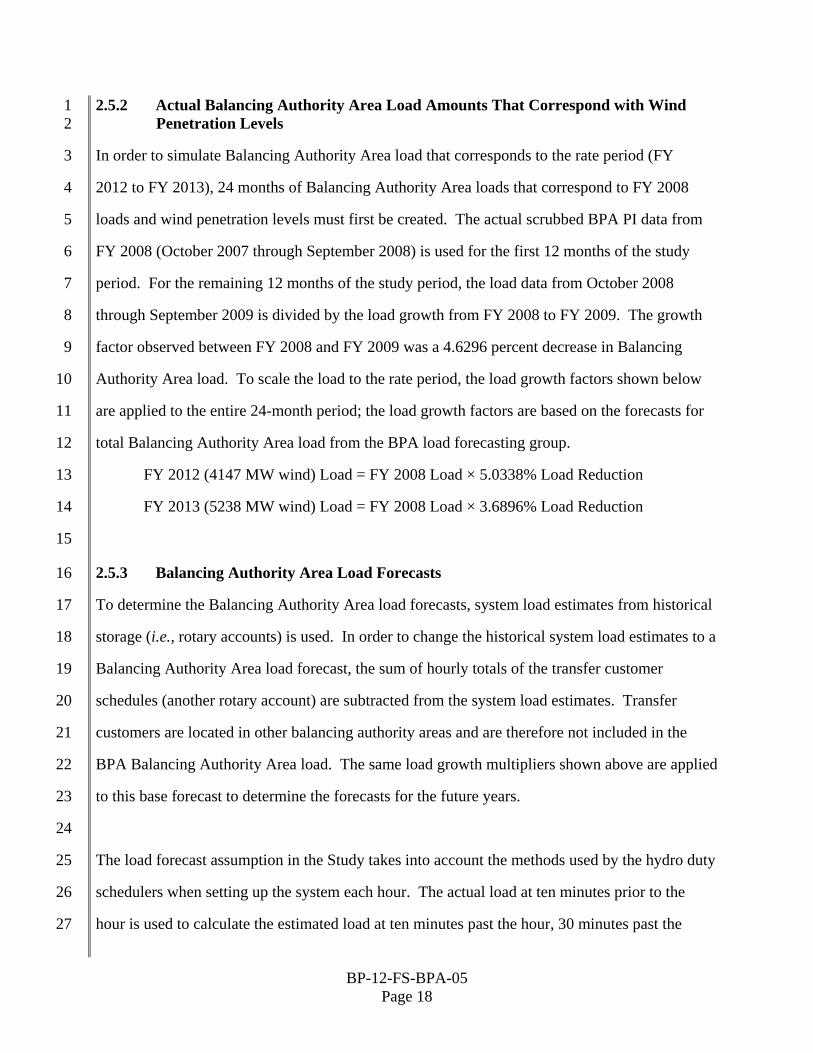
2.5.2 Actual Balancing Authority Area Load Amounts That Correspond with Wind 1 Penetration Levels 2

3

4

5

6

7

8

9

10

11

12

13

14

15

17

18

19

20

21

22

23

24

25

26

27

In order to simulate Balancing Authority Area load that corresponds to the rate period (FY

2012 to FY 2013), 24 months of Balancing Authority Area loads that correspond to FY 2008

loads and wind penetration levels must first be created. The actual scrubbed BPA PI data from

FY 2008 (October 2007 through September 2008) is used for the first 12 months of the study

period. For the remaining 12 months of the study period, the load data from October 2008

through September 2009 is divided by the load growth from FY 2008 to FY 2009. The growth

factor observed between FY 2008 and FY 2009 was a 4.6296 percent decrease in Balancing

Authority Area load. To scale the load to the rate period, the load growth factors shown below

are applied to the entire 24-month period; the load growth factors are based on the forecasts for

total Balancing Authority Area load from the BPA load forecasting group.

FY 2012 (4147 MW wind) Load = FY 2008 Load × 5.0338% Load Reduction

FY 2013 (5238 MW wind) Load = FY 2008 Load × 3.6896% Load Reduction

2.5.3 Balancing Authority Area Load Forecasts 16

To determine the Balancing Authority Area load forecasts, system load estimates from historical

storage (i.e., rotary accounts) is used. In order to change the historical system load estimates to a

Balancing Authority Area load forecast, the sum of hourly totals of the transfer customer

schedules (another rotary account) are subtracted from the system load estimates. Transfer

customers are located in other balancing authority areas and are therefore not included in the

BPA Balancing Authority Area load. The same load growth multipliers shown above are applied

to this base forecast to determine the forecasts for the future years.

The load forecast assumption in the Study takes into account the methods used by the hydro duty

schedulers when setting up the system each hour. The actual load at ten minutes prior to the

hour is used to calculate the estimated load at ten minutes past the hour, 30 minutes past the


hour, and 50 minutes past the hour. This is the same calculation performed by the software used

by the schedulers when setting up the system for the next hour. The inputs to these estimates are

the load at ten minutes prior to the hour and the load forecasts for the current hour and the next

two hours.

1

2

3

4

5

7

8

9

10

11

14

15

16

17

18

19

20

21

22

23

24

25

26

2.6 Wind Scheduling Accuracy Assumption 6

The scheduling accuracy of the wind fleet during the rate period is assumed to be equivalent to a

30-minute persistence measure. Under this assumption, the schedule for a wind facility for a

given hour equals the one-minute average of the actual generation of the facility 30 minutes prior

to the hour.

2.7 Balancing Reserve Capacity Requirements Methodology 12

2.7.1 Base Methodology 13

The methodology for forecasting the balancing reserve capacity requirements requires the

following one-minute average datasets: actual Balancing Authority Area load, Balancing

Authority Area load forecast, the total hydroelectric generation, the total hydroelectric schedule,

the total Federal thermal generation (Columbia Generating Station or CGS), the total Federal

thermal schedule, the total non-Federal thermal generation, the total non-Federal thermal

schedule, actual total wind generation, and total wind generation forecast. Each of these datasets

is obtained or calculated in the manner described in sections 2.2 through 2.6. Using these

datasets, the actual load net generation (actual Balancing Authority Area load minus actual total

hydroelectric generation minus actual total Federal thermal generation minus total actual non-

Federal thermal generation minus actual total wind generation) is determined on a minute-by-

minute basis. Then the load net generation forecast (Balancing Authority Area load forecast

minus actual total hydroelectric schedule minus actual total Federal thermal schedule minus total

actual non-Federal thermal schedule minus total wind generation forecast) is determined on a


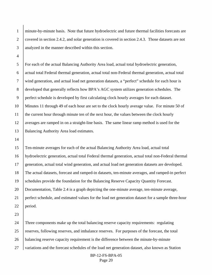
minute-by-minute basis. Note that future hydroelectric and future thermal facilities forecasts are

covered in section 2.4.2, and solar generation is covered in section 2.4.3. Those datasets are not

analyzed in the manner described within this section.

1

2

3

4

5

6

7

8

9

10

11

12

13

14

15

16

17

18

19

20

21

22

23

24

25

26

27

For each of the actual Balancing Authority Area load, actual total hydroelectric generation,

actual total Federal thermal generation, actual total non-Federal thermal generation, actual total

wind generation, and actual load net generation datasets, a “perfect” schedule for each hour is

developed that generally reflects how BPA’s AGC system utilizes generation schedules. The

perfect schedule is developed by first calculating clock hourly averages for each dataset.

Minutes 11 through 49 of each hour are set to the clock hourly average value. For minute 50 of

the current hour through minute ten of the next hour, the values between the clock hourly

averages are ramped in on a straight-line basis. The same linear ramp method is used for the

Balancing Authority Area load estimates.

Ten-minute averages for each of the actual Balancing Authority Area load, actual total

hydroelectric generation, actual total Federal thermal generation, actual total non-Federal thermal

generation, actual total wind generation, and actual load net generation datasets are developed.

The actual datasets, forecast and ramped-in datasets, ten-minute averages, and ramped-in perfect

schedules provide the foundation for the Balancing Reserve Capacity Quantity Forecast.

Documentation, Table 2.4 is a graph depicting the one-minute average, ten-minute average,

perfect schedule, and estimated values for the load net generation dataset for a sample three-hour

period.

Three components make up the total balancing reserve capacity requirements: regulating

reserves, following reserves, and imbalance reserves. For purposes of the forecast, the total

balancing reserve capacity requirement is the difference between the minute-by-minute

variations and the forecast schedules of the load net generation dataset, also known as Station


Control Error (SCE). The regulating reserves component is defined by the minute-by-minute

variations around the ten-minute clock average of the load net generation dataset. The following

reserves component is defined by the difference minute by minute between the ten-minute clock

average of the load net generation dataset and the associated perfect schedule. The imbalance

reserves component is defined as the incremental amount of additional following reserve that

results from using forecast schedules instead of perfect schedules. Documentation, Table 2.4

reflects the regulating reserves, following reserves, and imbalance reserves components in terms

of the relationships between the one-minute averages, ten-minute averages, perfect schedules,

and estimated schedules for a sample three-hour period.

1

2

3

4

5

6

7

8

9

10

12

13

14

15

16

17

18

19

20

21

22

23

24

25

26

2.7.2 Time Series of Studies 11

To forecast the overall balancing reserve capacity requirements, an inc and dec requirement is

calculated for the regulating reserves, following reserves, and imbalance reserves components

for each of the actual Balancing Authority Area load, actual total hydroelectric generation, actual

total Federal thermal generation, actual total non-Federal thermal generation, actual total wind

generation, and actual load net generation datasets. The inc and dec amounts are calculated for

the different amounts of wind penetration and load for FY 2012–2013.

Using percentile distribution, values from the upper and lower 0.25 percent are discarded for

each component, leaving 99.5 percent of the values for calculating the capacity requirements of

the BPA Balancing Authority Area. This produces a forecast of the balancing reserve capacity

that BPA needs to meet its balancing requirements 99.5 percent of the time. Using 99.5 percent

of the values is generally consistent with the historical method of using three standard deviations

to calculate requirements (using three standard deviations would result in using 99.7 percent of

the values in the calculations). By using 99.5 percent of the values, another 0.2 percent of

variation that would otherwise factor into the forecast is not accounted for; however, BPA has


performed well in meeting the requirements of the North American Electric Reliability

Corporation and Western Electricity Coordinating Council balancing standards, and therefore it

is assumed that an additional 0.2 percent of the movement in the Balancing Authority Area is

absorbed from this point forward. This decreases the overall balancing reserve capacity

requirement slightly.

1

2

3

4

5

6

7

8

9

10

11

12

13

14

15

16

17

18

19

20

21

22

23

24

25

26

Using 99.5 percent of values for the load net generation dataset, the balancing reserve capacity

requirement forecast is calculated for the total balancing reserve capacity requirement, the total

regulation requirement, and the total following requirement. The total imbalance requirement is

calculated as the remainder of the total balancing reserve capacity requirement minus the total

regulation requirement minus the total following requirement. The equations below describe

these calculations. Section 2.7.3 describes the methodology used to disaggregate the balancing

reserve capacity requirements for each resource and reserve type (i.e., load regulation inc, wind

regulation inc, hydro regulation inc, etc.).

Total Reserve Requirement

Total inc = p9975(Total SCE)

Total dec = p0025(Total SCE)

Total Regulation Requirement (Reg)

Total Reg inc = p9975(Total Regulation)

Total Reg dec = p0025(Total Regulation)

Total Following Requirement (Fol)

Total Fol inc = p9975(Total Following)

Total Fol inc = p0025(Total Following)

Total Imbalance Requirement (Imb)

Total Imb inc = Total inc - Reg inc - Fol inc

Total Imb dec = Total dec - Reg dec - Fol dec


Where p9975 is the 99.75% percentile distribution 1

2

3

4

5

6

7

8

9

11

12

13

14

15

16

17

18

19

20

21

22

23

24

25

26

27

p0025 is the 0.25% percentile distribution

The Study also includes a forecast of the balancing reserve capacity requirements that BPA

needs to meet its balancing requirements 99.7 percent of the time. The forecast using

99.7 percent results in a slightly larger balancing reserve capacity requirement, equivalent to the

historical probability method of three standard deviations. The 99.7 percent forecast was

developed using the same methods and data as described in this Study, except that the

0.15 percent of each inc and dec component was discarded in the time series study.

2.7.3 Allocating the Total Balancing Reserve Capacity Requirement Between 10 Generation and Load

Once the forecast of the total balancing reserve capacity requirements is determined, the total is

allocated between the contributions from generation type and load. The goal in determining this

allocation is to find a statistically valid method under which the sum of the parts always equals

the total (e.g., Federal thermal regulation inc + non-Federal thermal regulation inc + wind

regulation inc + hydro regulation inc + load regulation inc = total regulation inc). To do this in a

statistically accurate manner, incremental standard deviation (ISD) is employed to allocate

reserves to load and generation type based upon how each contributes to the joint load-

generation regulating reserve requirement, following reserve requirement, and imbalance reserve

requirement.

The ISD measures how much load and generation each contributes to the total load net

generation balancing reserve capacity need based on how sensitive the total balancing reserve

capacity need is with respect to the individual load and generation components. Stated

differently, ISD shows how much the total balancing reserve capacity standard deviation changes

given a one-megawatt change in the load and/or generation standard deviation. ISD recognizes

the diversification between the load and generation error signals, i.e., the fact that the load and


generation error signals do not always move in the same direction. The result of diversification

is a joint load-generation balancing reserve capacity requirement that is less than the sum of the

individual requirements for load and generation. Through the ISD, the joint load-generation

balancing reserve capacity requirement is disaggregated into the component contributions of load

and generation. The result of the decomposition is a total balancing reserve capacity requirement

fully reflecting the impacts of signal diversity. Having used the ISD method, the sum of the

individual balancing reserve capacity requirements now equals the total balancing reserve

capacity requirement.

1

2

3

4

5

6

7

8

9

10

11

12

13

14

15

16

17

18

19

20

21

22

23

24

25

26

27

In order to accurately capture the diversification between load and generation and still attribute

appropriate shares of the balancing reserve capacity requirements to each generation type and to

load, the error signals for all balancing reserve capacity components are sorted into 24 hourly

bins based on time of day. For example, total regulation, load regulation, wind regulation, hydro

regulation, non-Federal thermal regulation, and Federal thermal regulation are all sorted among

24 bins: one bin for all data points falling in hour ending 1 (HE1), one bin for all data points

falling in hour ending 2 (HE2), and so on. ISD is performed on each hourly bin to determine a

balancing reserve capacity requirement for every component. An example of the ISD

calculations is presented in Documentation, Table 2.5. Then the maximum of the 24 hourly bin

percentile distributions is found. Finally, the total reserve requirements calculated using the

formulas in section 2.7.2 are disaggregated using the ratio of each component’s maximum

24-hour requirement to the sum of all of the maximum 24-hour requirements. An example of

these calculations for the load regulating inc reserve component is presented in Documentation,

Table 2.6.

The data used to determine the balancing reserve capacity requirements are not normally

distributed. The distribution of the data is not symmetrical; as a result, using the ISD to allocate

between load and generation requires an additional step to correctly infer the balancing reserve


capacity requirement at the desired percentile. The current balancing reserve capacity

requirement is calculated at the 99.75th percentile for incs and 0.25th percentile for decs, which

equates to +/- 2.81 standard deviations (z-value), if assuming a standard normal distribution.

That is, data that are normally distributed have 99.75 percent of their values occurring at 2.81 or

fewer standard deviations from the mean. The distance or number of standard deviations from

the mean is at times referred to as the z-value. Rather than assuming that the load and generation

type error signals are standard normal and using a z-value of +/- 2.81 for purposes of the

Balancing Reserve Capacity Quantity Forecast in this case, the z-value associated with the

99.75th percentile and the 0.25th percentile is calculated based on the empirical data.

Specifically, each of the actual 99.75th percentile inc and the 0.25th percentile dec data is

divided by the standard deviation of the component error signals to determine an “actual” inc and

dec z-value. Multiplying the “actual” z-value by the ISD results in a disaggregated reserve

requirement adjusted for the non-normality in the empirical data while accounting for the

diversity among the signals.

1

2

3

4

5

6

7

8

9

10

11

12

13

14

15

17

18

19

20

21

22

23

24

25

26

2.7.4 Determining the Imbalance Reduction for Self-Supply 16

Once the allocation of the forecast of the total balancing reserve capacity requirement is

determined, the entire allocation calculation is repeated with the wind generation/schedule

signals split into separate self-supply and non-self-supply generation/schedule signals. The

resulting self-supply imbalance reserve amount determines the reduction in balancing reserve

capacity due to self-supply. This reduction is applied to the wind imbalance reserves, the BPA

Balancing Authority Area imbalance reserves, and the BPA Balancing Authority Area total

balancing reserve capacity requirement. Assumptions regarding the wind facilities participating

in self-supply of imbalance reserves for the FY 2012–2013 rate period are based on the data that

is available for the current Customer-Supplied Generation Imbalance pilot participation.

Customers that elected (by May 1, 2011) to participate in self-supply of the imbalance portion of


their balancing reserve capacity requirement for the FY 2012–2013 rate period are reflected in

the Study.

1

2

3

5

6

7

8

9

10

11

12

13

14

15

16

17

18

19

20

21

22

23

24

25

2.8 Committed Intra-Hour Scheduling Pilot 4

The Study includes a separate forecast of the potential balancing reserve capacity requirement

reductions associated with committed intra-hour scheduling by the entire wind fleet in BPA’s

Balancing Authority Area. To develop this forecast, the study assumes that all of the wind

projects in the BPA Balancing Authority Area schedule every 30 minutes instead of every 60

minutes, with accuracy based on 30-minute persistence scheduling. The study assumes standard

ramps of ten minutes before and after the top of the hour and five minutes before and after mid-

hour. The study uses the same methodology as described in section 2.7, assuming a total

balancing reserve capacity of 99.5 percent and no self-supply. The full benefit of wind

generation participating in committed intra-hour scheduling pilot would be seen in the reduction

of the total balancing reserve capacity for BPA’s Balancing Authority Area, because committed

intra-hour scheduling by the entire wind fleet would reduce the aggregate load net generation

error for the Balancing Authority Area. Documentation, Tables 2.25, columns G and H. The

study analyzes the reduced aggregate error for reserve requirements and allocates the

requirements to the different reserve components (regulation, following, and imbalance) and

reserve types (load, thermal generation, and wind generation) using incremental standard

deviation. The savings seen by the reduction of the total balancing reserve capacity for the

Balancing Authority are then credited against the forecast reserve requirement for wind.

The study results for committed intra-hour scheduling by the entire wind fleet can be found in

Documentation, Table 2.26, columns G and H, that shows the average reduction in the forecast

of the total balancing reserve capacity requirement for the rate period is approximately 34


percent. For those entities participating in committed intra-hour scheduling pilot, an adjustment

will be made to give a credit of 34 percent of the VERBS rate.

1

2

3

5

6

7

8

9

10

11

12

13

14

15

16

17

18

19

20

21

22

23

24

25

26

2.9 Study of Quality of Service Levels in Excess of 99.5 Percent 4

The Study also quantifies the additional inc balancing reserve capacity needed above the

99.5 percent level to achieve different frequencies of DSO 216 under-generation tag curtailment

events. To perform this analysis, estimates of DSO 216 under-generation tag curtailment

frequency were needed for incremental increases of the inc balancing reserve capacity allocated

to wind above the 99.5 percent level of service. Using the one-minute time series data for

generation and load, and schedules for load, wind, hydro generation, Federal thermal generation,

and non-Federal thermal generation, an aggregate “load net generation” SCE was calculated by

subtracting the “load net generation” schedules from the “load net generation” actuals. The

aggregate “load net generation” SCE was analyzed to capture all of the times in which a DSO

216 event would have occurred. The following criteria were used:

The threshold for analysis was defined as 90 percent of the total balancing authority area

inc balancing reserve requirement, because that is the threshold at which DSO 216

triggers.

Top-of-the-hour ramps from ten minutes before to ten minutes after the hour were

excluded from the analysis, pursuant to the current DSO 216 implementation.

One event per clock hour (per direction) was allowed, because a DSO 216 directive

carries through until top of the hour. The study assumed that an inc (under-generation)

and a dec (over-generation) event could occur in the same clock hour.

Events lasting multiple clock hours were split into multiple events.

Each month of the rate period was analyzed separately using its associated 24 months of one-

minute data with the forecast installed wind capacity and load growth. The results for


augmenting the wind inc balancing reserve capacity for entire balancing authority are presented

in Documentation, Tables 2.27 and 2.28. The results are presented as the multiples of additional

reserves needed above the 99.5 percent inc wind balancing reserve capacity requirement

(Documentation, Table 2.9) that correspond to a particular number of DSO 216 curtailments.

For example, the average inc wind balancing reserve capacity requirement without Self Supply is

620 MW, and the average magnitude of additional reserves needed to lower the DSO 216 tag

curtailment frequency to 11 events per year is 0.9, so an average of 1,178 MW (620 MW × 1.9)

of total inc wind balancing reserve capacity would be needed to achieve this DSO 216 frequency.

1

2

3

4

5

6

7

8

9

11

12

13

14

15

16

17

18

19

20

21

22

23

24

25

2.10 Results 10

The Study forecasts the balancing reserve capacity requirements for the three different

components of balancing reserve capacity: regulating reserves, following reserves (with perfect

schedules), and imbalance reserves (following reserve with actual schedules and estimates).

Other non-AGC generation was accounted for in the Balancing Reserve Capacity Quantity

Forecast in the following ways:

Hydroelectric generation balancing reserve capacity requirements are incorporated into

the load balancing reserve capacity requirement.

Federal thermal generation balancing reserve capacity requirements are incorporated into

the load balancing reserve capacity requirement.

Non-Federal thermal generation balancing reserve capacity requirements are assessed a

separate balancing reserve capacity requirement.

Solar generation balancing reserve capacity requirements are incorporated into the wind

balancing reserve capacity requirement.



1

2

3

4

5

6

7

8

9

10

11

12

13

14

15

16

17

18

19

20

21

22

23

24

25

26

Documentation, Tables 2.7 through 2.24 include the results of the Balancing Reserve Capacity

Quantity Forecast. All of these tables reflect the results assuming that wind generators are

scheduling consistent with a 30-minute persistence model. Documentation, Tables 2.7 through

2.10 include the inc and dec amounts for each component of the total balancing reserve capacity

requirement, the load balancing reserve capacity requirement, the wind balancing reserve

capacity requirement, and the non-Federal thermal generation balancing reserve capacity

requirement, respectively. These requirements cover the balancing reserve capacity

requirements for 99.5 percent of the time and assume no self-supply of imbalance capacity by

any generators during the rate period. Documentation, Tables 2.11 through 2.14 provide the

same information for load and each type of generation at the 99.7 percent probability and

assuming no self-supply. Documentation, Tables 2.15 through 2.24 include results of the

Balancing Reserve Capacity Quantity Forecast assuming a level of imbalance reserve self-supply

as described in section 2.7.4.

The results for committed intra-hour scheduling by the entire wind fleet can be found in

Documentation, Tables 2.25 and 2.26. The results for the study of quality of service levels in

excess of 99.5 percent, which quantifies the requirements for augmenting the wind inc balancing

reserve capacity of the entire balancing authority, are presented in Documentation, Tables 2.27

and 2.28.

3. BALANCING RESERVE CAPACITY COST ALLOCATION METHODOLOGY 1

2

4

5

6

7

8

9

10

11

12

13

14

15

16

17

18

19

20

21

22

23

24

25

26

27

3.1 Introduction 3

The Federal Columbia River Power System (FCRPS) is used to provide balancing reserve

capacity for various Ancillary and Control Area Services. This section of the Study describes the

allocation of embedded costs, direct assignment costs, and variable costs for Regulating Reserve,

Load Following Reserve, Dispatchable Energy Resource Balancing Service (DERBS) Reserve,

and Variable Energy Resource Balancing Service (VERBS) Reserve. Regulating Reserve is

used to balance loads in the BPA Balancing Authority Area on a moment-to-moment basis.

Load Following Reserve is used to balance loads through the operating hour. DERBS Reserve is

comprised of regulating, following, and imbalance reserves that are used to balance dispatchable

generation in the BPA Balancing Authority Area moment-to-moment and through the operating

hour. VERBS Reserve, formerly known as Wind Balancing Service Reserve, is also comprised

of regulating, following, and imbalance reserves that are used to balance the variable energy

resource generation in the BPA Balancing Authority Area moment-to-moment and through the

operating hour.

The embedded cost allocation is based on the embedded costs of a defined portion of the existing

FCRPS. Embedded costs are explained in detail in section 3.2. Direct assignment costs are a

narrowly defined set of costs that will be recovered through the VERBS rate. The direct

assignment costs are explained in detail in section 3.3. The variable cost methodology

determines the cost associated with the loss of efficiency caused by providing balancing reserve

capacity from the FCRPS. Variable costs are explained in detail in section 3.4. The cost

allocation for balancing reserve capacity is the sum of associated embedded costs, applicable

direct assignment costs, and variable costs. The costs for Regulating Reserve, DERBS Reserve,

and VERBS Reserve are assigned to Transmission Services (TS) to be recovered through the

Ancillary and Control Area Services rate schedule, which is described in section 10 of this


Study. The cost associated with Load Following Reserve is not assigned to TS; rather, these

costs remain as part of the power rates revenue requirement. The cost of Contingency Reserves,

referred to in this study as Operating Reserves, is also assigned to TS. The Operating Reserve

cost allocation is described in detail in section 4.

1

2

3

4

5

6

7

8

9

10

11

12

13

14

15

16

17

18

19

20

21

22

23

24

25

26

27

Forecast TS revenue from the sale of Regulation, DERBS, and VERBS reserves is treated as a

revenue credit and allocated to the composite cost pool in the calculation of power rates. See the

Power Rates Study, BP-12-FS-BPA-01, section 4.

The assumptions for the base case in this section of the study are: (1) a quantity of balancing

reserve capacity that allows BPA to support variable energy resources 99.5 percent of the time;

(2) the wind fleet schedules at a 30-minute persistence scheduling accuracy level; and (3) a

certain quantity of the imbalance portion of the VERBS Reserve will be customer-supplied (i.e.,

self-supplied). The amount of balancing reserve capacity required to provide Regulating, Load

Following, DERBS, and VERBS Reserves is described in section 2.

In addition to the Balancing Reserve Capacity Quantity Forecast, BPA uses other inputs in its

cost allocation methodologies. These inputs include the net revenue requirement for balancing

reserve capacity for embedded costs from the Power Revenue Requirement Study

Documentation, BP-12-FS-BPA-02A, section 2.3; the regulated hydro project information from

the Power Loads and Resources Study, BP-12-FS-BPA-03, section 3.1.2.1; the 120-hour

regulated hydro peaking capacity developed from an Hourly Operation and Scheduling

Simulator (HOSS) capacity analysis that forecasts the amount of 120-hour peaking capacity

available from regulated hydro energy production under certain water conditions; the amount of

Operating Reserve required by BPA from section 4; and the market price forecast from the

Power Risk and Market Price Study, BP-12-FS-BPA-04, section 2.


This Study introduces several changes to the cost allocation methodologies, including: (1) direct

assignment to VERBS of costs for the Wind Integration Team (WIT); (2) direct assignment to

VERBS of costs for a dec Acquisition Pilot; (3) streamlined treatment of deriving the 120-hour

peaking capacity of the Big 10 hydro projects; and (4) a new cost allocation for DERBS Reserve.

1

2

3

4

5

7

8

9

10

11

12

13

14

15

16

17

18

19

20

22

23

24

25

26

27

3.2 Embedded Cost Allocation Methodology 6

The embedded unit cost of Regulating Reserve, DERBS Reserve, and VERBS Reserve is

calculated by taking the costs associated with the Big 10 hydro projects (described in

section 3.2.1) and dividing those costs by the average annual capacity amount of the Big 10

hydro projects (adjusted for other requirements). The costs associated with the Big 10 hydro

projects are power-related costs on a project-specific basis, an allocation of fish costs and general

and administrative costs, and three revenue credit adjustments. The capacity amount is

determined using BPA’s hydro simulation model, HYDSIM, and the HOSS model. These

models are used to compute the average annual 120-hour peaking capacity of the regulated hydro

system. These 120-hour peaking capacity amounts are averaged for each month. This results in

an annual average amount of reliable monthly sustained capacity that will be available for

operational planning purposes. The calculated embedded unit cost is then multiplied by the

balancing reserve capacity quantity forecast for each type of reserve to yield the embedded cost

allocation for that type of balancing reserve capacity.

3.2.1 Description of the Portion of the FCRPS Used to Provide Balancing Reserve 21 Capacity

BPA has 14 Federal hydro projects whose coordinated individual generation forecasts are

modeled in BPA’s regulated hydro simulation model, HYDSIM. These projects are collectively

called Federal system regulated hydro projects and are listed in Documentation, Table 3.2.

Within this group, 10 projects are used by BPA to provide balancing reserve capacity for

regulating, load following, DERBS, and VERBS Reserves. The 10 projects are Grand Coulee,


Chief Joseph, Lower Granite, Little Goose, Lower Monumental, Ice Harbor, McNary, John Day,

The Dalles, and Bonneville. These 10 projects are referred to as the “Big 10 projects” because

they are controlled in real time by Automatic Generation Control (AGC) and provide balancing

reserve capacity. AGC is the computer system connected to these generating resources that

allows them to respond immediately to the AGC computer signal to provide sufficient regulating

margin to allow the Balancing Authority Area to meet NERC Control Performance Criteria.

1

2

3

4

5

6

7

9

10

11

12

13

14

15

16

17

18

19

20

21

22

23

24

25

26

3.2.2 Determining the Amount of Capacity Provided by the FCRPS 8

The Federal system regulated hydro projects are hydraulically linked in the Columbia River

Basin. Hydro energy and capacity production at these projects is directly related to: (1) the

amount of water in the Columbia River Basin; (2) power and non-power requirements, such as

flood control, fish operations, and recreation; (3) reliability and reserve requirements, such as the

balancing reserve capacity used for VERBS and Load Following; and (4) turbine availability,

which is the number of units not out of service due to planned maintenance and unplanned

outages. The coordinated energy production for these storage projects is forecast by HYDSIM

for each of the 14 periods used in the hydro studies. Each month of a fiscal year is a period

except for the months of April and August, which are both split into two periods because the

natural streamflows are significantly different in the first half and second half of these months.

HYDSIM produces average energy amounts for each of the 14 periods by fiscal year for the

70 water years of record (October 1928 through September 1998) but does not produce forecasts

of Heavy Load Hour (HLH) and Light Load Hour (LLH) energy amounts by period. Instead, the

hourly detail is produced by BPA’s HOSS model. The combination of the two hydro simulation

models (HYDSIM and HOSS) is used to quantify the amount of available capacity for the

14 Federal regulated hydro resources. Though the HYDSIM and HOSS models are operated for

the 70 water years of record, the focus of the cost allocation methodology is the 1958 water year,


which represents an average water condition. These processes are described in the following

sections.

1

2

3

5

6

7

8

9

10

11

12

13

14

15

16

17

18

19

20

21

22

23

24

25

3.2.3 Source and Description of Inputs and Outputs of the HYDSIM Model 4

HYDSIM simulates monthly energy hydro production under the physical characteristics and

limits placed on the modeled Columbia River Basin projects, including hard project constraints

(e.g., flow limits, elevation limits), project outages (planned and forced outages), balancing

reserve capacity requirements, one-percent efficiency restrictions, and non-power requirements

(flood control, variable draft limits, fish operations pursuant to the Biological Opinions, and

Canadian Treaty operations). HYDSIM models these hydro projects to meet system load while

continuing to meet Pacific Northwest regional power and non-power requirements for the 70

water years of record (October 1928 through September 1998). Power Loads and Resources

Study, BP-12-FS-BPA-03, section 3.1.2.1.

The Federal system regional hydro projects are termed “regulated” hydro projects, because their

coordinated operation is modeled in HYDSIM. BPA uses the HYDSIM energy generation

forecasts for the 14 regulated hydro projects as the base energy for analyzing capacity in the cost

allocation methodology. Further information on the operation of HYDSIM is presented in the

Power Loads and Resources Study, BP-12-FS-BPA-03, section 3.1.2.1. The hydro energy

generation forecast for the 14 Federal system regulated hydro projects under 1958 water

conditions is a primary factor in the determination of the 120-hour hydro peaking capacity

relationship derived in HOSS.


3.2.4 Source and Description of HOSS and Modifications 1

The embedded cost methodology focuses on availability of balancing reserve capacity from the

Federal system regulated hydro projects. To analyze capacity, the HOSS model simulates hourly

operation of the Federal system to meet hourly loads for each period of the 70 historical water

conditions for the study period. The outputs of HOSS are not directly used for ratesetting

purposes. Rather, monthly Federal system regulated hydro generation energy relationships are

developed to provide monthly HLH energy, LLH energy, and 120-hour hydro peaking capacity

using outputs from HOSS, which are explained in more detail in sections 3.2.5 and 3.2.6.

2

3

4

5

6

7

8

9

10

11

12

13

14

15

16

17

18

19

20

21

22

23

24

25

26

The HOSS model uses HYDSIM monthly project flows, initial and ending conditions, reserve

requirements, and other power and non-power constraints that are provided by the Power Loads

and Resources Study, BP-12-FS-BPA-03, section 3.1.2.1. HOSS incorporates hourly versions of

the input data for Regulating Reserve, Operating Reserve, Load Following Reserve, DERBS

Reserve, and VERBS Reserve. These are computed once for each of the 14 periods in a year,

and these values are used under all 70 water conditions. These reserve amounts affect the

generating capacity and 120-hour hydro peaking capacity available.

The HYDSIM and HOSS inputs for Operating Reserve are calculated consistent with the

reserves forecast in the Operating Reserve Cost Allocation in section 4 (i.e., seven percent of

thermal and five percent of hydro, wind, and other resources for FY 2012, and three percent of

the load and three percent of net generation for FY 2013), with one difference. Instead of using

averages for the Operating Reserve requirements, the Operating Reserve requirement that is used

in HOSS and HYDSIM is calculated based on historical peak Balancing Authority Area

generation at the 95th percentile by month. The peak 95th percentile is used instead of an

average, because Operating Reserve constrains the system at high levels of generation. If HOSS

and HYDSIM assumed an average Operating Reserve requirement, the study result would not


adequately cover the Operating Reserves required for actual operations during periods of high

generation.

1

2

3

4

5

6

7

8

9

10

11

12

13

14

15

16

17

18

19

20

21

22

23

24

25

26

The other inputs for balancing reserve capacity used in the HYDSIM and HOSS models are

based on the Regulating Reserve, Load Following Reserve, DERBS Reserve, and VERBS

Reserve forecast in the Balancing Reserve Capacity Quantity Forecast, described in section 2.

Table 3.4 contains the total monthly inc and dec balancing reserve capacity amounts of

Regulating Reserve, Load Following Reserve, DERBS Reserve, and VERBS Reserve used as

inputs to HYDSIM and HOSS.

The HOSS and HYDSIM models use both the inc and dec balancing reserve capacity amounts.

As described in the Balancing Reserve Capacity Quantity Forecast in section 2, inc balancing

reserve capacity is the capacity available to ramp up generation to meet increasing within-hour

load or decreasing within-hour generation output. Dec balancing reserve capacity is the

generating capacity available to ramp down to meet increasing within-hour generation output or

decreasing within-hour load. In HOSS and HYDSIM, the inc requirement is treated as a

reduction to available capacity to generate power, and the dec requirement is treated as an

increase in the minimum generation requirement at Grand Coulee, Chief Joseph, McNary, John

Day, and The Dalles.

The resulting HOSS model generation study maximizes HLH Federal system hydro generation

and creates hourly projections of hydro generation, by period, for each of the 70 water conditions

of the study period. These estimates provide the basis for: (1) Federal system hydro energy

relationships that provide HLH and LLH energy splits that are shown in the Power Loads and

Resources Study, BP-12-FS-BPA-03, section 3.1.2.1 and Power Loads and Resources

Documentation, BP-12-FS-BPA-03A, Tables 2.1.2 and 2.1.3, and inputs to the Power Risk and


Market Price Study, BP-12-FS-BPA-04, section 2; and (2) the 120-hour peaking capacity of the

Federal hydro system for this Study, described below.

1

2

3

5

6

7

8

9

10

11

12

13

14

15

16

17

18

19

20

21

22

23

24

25

26

3.2.5 120-Hour Federal System Hydro Capacity 4

The hourly output data from HOSS provides BPA data to compute Federal system hydro energy

to capacity relationships for each of the 14 periods and 70 water conditions for the study period.

For the FY 2012–2013 rate period, HOSS 120-hour peaking capacity estimates represent the

amount of capacity on the Federal hydro system that is available to reliably serve Federal system

load obligations after meeting balancing reserve capacity obligations; and power and non-power

requirements within any period or water condition. It is not meant to represent a time of system

stress to meet large weather deviations, additional reserve obligations, or other extreme

conditions on the Federal system. The 120-hour peaking capacity quantification is the same

capacity planning standard used in BPA’s short-term planning.

One hundred twenty-hour hydro capacity is defined as the average hourly HOSS Federal system

hydro generation that is calculated from the highest six hours of generation for each of five

weekdays of a four-week period. The split months of April and August use two 60-hour periods

representing the highest six hours of generation for each of the five weekdays of each two-week

period. The generation is calculated for all water conditions to obtain hydro energy to 120-hour

peaking capacity curve relationships for the 70 water conditions for the study period. This Study

uses only 1958 water conditions, however, which approximate average water conditions.

The 120-hour hydro peaking capacity values are constructed using the output of HOSS

(calculation of these relationships is described in greater detail below) and are applied to the

14-period average energy amounts produced by HYDSIM. These 120-hour capacity values are

averaged for FY 2012–2013, and this average is considered to be the amount of reliable monthly


120-hour hydro peaking capacity that would be available for operational planning purposes for

this Study.

1

2

3

5

6

7

8

9

10

11

12

13

14

15

16

17

18

19

20

21

22

24

25

26

3.2.6 Detailed Development of 120-Hour Hydro Peaking Capacity 4

Summaries of the hourly output of HOSS are used to develop relationships between the average

energy during each of the 14 periods of the year and the associated 120-hour hydro peaking

capacity for each of the 70 historical water years. These relationships are created through curves

that define peaking capacity as a function of monthly energy for each of the 70 hydro conditions.

The data from HOSS is entered into an Excel spreadsheet, and the curve-fitting function in

Microsoft Excel is used to generate a peaking capacity equation for each period that reflects the

120-hour peaking capacity of the system for any given energy content for that period. The

equation will produce a 120-hour peaking amount (Y) for any input average energy amount

(variable X). Table 3.3 shows an example of the 120-hour peaking capacity curves that are

developed from the HOSS output. For any amount of Federal regulated hydro energy, there is an

associated 120-hour Federal hydro capacity that is available to meet Federal obligations.

The 120-hour capacity equations (curves) are developed for each of the 14 periods of the year.

For the purpose of this Study, 1958 water conditions were selected to represent average water

conditions for the regulated hydro energy to 120-hour capacity relationship. The regulated hydro

energy for 1958 water conditions was an input that was applied to the 120-hour capacity

equations to produce the 120-hour hydro peaking capacity for each period.

3.2.7 Big 10 Hydro 120-Hour Peaking Capacity for the Embedded Cost Methodology 23

The 120-hour hydro peaking capacity methodology described above calculates the available

capacity from the 14 Federal system regulated hydro projects. To determine the 120-hour hydro

peaking capacity of the Big 10 hydro projects used in the embedded cost methodology, the


following steps are taken: (1) the capacity amounts for the regulated hydro projects are

converted into annual averages for the FY 2012–2013 rate period (Table 3.1, lines 2, 5, and 8);

(2) the annual average capacity for regulated hydro is adjusted for transmission losses by

applying the capacity transmission loss factor of 3.35 percent which was provided by BPA’s

Transmission Services; and (3) because the HOSS model treats Federal regulated hydro as a

system, not as individual hydro projects, to determine the 120-hour capacity amount for the Big

10 hydro projects the proportion of the 14 regulated hydro projects that represents the Big 10

hydro projects is calculated. The Big 10 projects represent 93 percent of the 120-hour peaking

capacity produced by all 14 regulated hydro projects, as shown in Table 3.2, line 17.

1

2

3

4

5

6

7

8

9

10

11

12

13

15

16

17

18

19

20

21

22

23

24

25

26

The 93 percent portion of the regulated hydro is used in the Regulating, DERBS, and VERBS

Reserves cost allocations, shown on Table 3.6, line 7.

3.2.8 Embedded Unit Cost Calculation 14

The embedded unit cost of Regulating, DERBS, and VERBS Reserves is calculated by taking the

embedded cost net revenue requirement associated with the Big 10 hydro projects and dividing

these costs by the 120-hour peaking capacity total system uses. The “total system uses” is the

sum of the Big 10 hydro projects’ 120-hour peaking capacity (adjusted for transmission losses)

and the forecast quantities for Regulating Reserve, Load Following Reserve, DERBS Reserve,

and VERBS Reserve. See Study, section 2, and Documentation, Table 2.16. See also Study,

section 4 and Documentation, Table 4.6, line 13. The embedded costs are allocated based on the

inc reserve forecast.

The Operating Reserve quantity used is adjusted to take into account that Supplemental (non-

spinning) Operating Reserve can be carried on projects in addition to the Big 10 hydro projects.

The Big 10 hydro projects comprise 91 percent of the hydro projects in the BPA Balancing


Authority Area capable of providing Operating Reserves. The hydro projects capable of

providing Operating Reserves are the regulated hydro projects and the independent hydro

projects within the BPA Balancing Authority Area. See the WP-10 Final Generation Inputs

Study, WP-10-FS-BPA-08, section 3.4. This is a different adjustment from the 93 percent

adjustment described above, which represents the Big 10 as a proportion of the 14 regulated

hydro projects. In this Supplemental Operating Reserve adjustment, the 91 percent represents

the portion of a larger subset of FCRPS hydro projects than the 14 regulated hydro projects. The

Supplemental Operating Reserve quantity is reduced by nine percent to account for the portion

that is carried on projects other than the Big 10 hydro projects. Documentation, Table 3.6, line 3.

1

2

3

4

5

6

7

8

9

10

12

13

14

15

16

17

18

19

20

21

22

23

24

25

26

3.2.8.1 Net Revenue Requirement Associated with the Big 10 Projects 11

The embedded cost net revenue requirement associated with the Big 10 hydro projects is

composed of: (1) power-related costs of the Big 10 hydro projects on a project-specific basis;

(2) an allocation of associated fish mitigation costs; (3) an allocation of administrative and

general expense; and (4) three specific revenue credits. Documentation, Table 3.5. The fish

mitigation costs and the general and administrative costs are not set on a project-specific basis,

so to allocate those costs to the Big 10 hydro projects, BPA takes 91 percent of these costs,

because, as stated above, the Big 10 projects comprise 91 percent of the hydro system in the

BPA Balancing Authority Area. The three specific revenue credits are 4(h)(10)(C) (non-

operations), Colville payment Treasury credit, and synchronous condensing. With the exception

of the revenue credit for synchronous condensing (Documentation, Table 3.5, line 18), the inputs

for Table 3.5 are described in the Power Revenue Requirement Study Documentation, BP-12-

FS-BPA-02A, section 2.3. The synchronous condensing costs are allocated to TS in a separate

calculation (described in section 5 of this Study), so they are removed to avoid double-counting.

The annual average net revenue requirement associated with the Big 10 projects for the rate

period is $876,768,000. Documentation, Table 3.5, line 19.


3.2.8.2 Calculation of the Embedded Unit Cost for Regulating, DERBS, and VERBS 1 Reserves 2

3

4

5

6

7

8

10

11

12

13

14

15

16

17

18

19

20

21

22

23

24

25

26

27

The annual average net revenue requirement of the Big 10 hydro projects of $876,768,000 is

divided by the total system uses of 10,929 MW to calculate the embedded unit cost of $6.69 per

kW per month for Regulating, DERBS, and VERBS Reserves. Documentation, Table 3.6. The

denominator is the sum of the inc reserve requirements supplied by the Big 10 hydro projects and

the 120-hour peaking capacity of the Big 10 hydro projects. Id. at lines 1-9.

3.2.8.3 Forecast of Revenue from Embedded Cost Portion of Regulating Reserve, VERBS 9 Reserve, and DERBS Reserve

The embedded cost revenue from providing Regulating Reserve is forecast by applying the unit

cost calculated above to the Regulating Reserve inc quantity forecast in Documentation,

Table 2.17, column F. The revenue forecast for the embedded cost portion is an average annual

amount of $4,816,800. Documentation, Table 3.6, line 14.

The embedded cost revenue from providing VERBS Reserve is forecast by applying the unit cost

calculated above to the VERBS inc reserve quantity forecast in Documentation, Table 2.18,

column L. The revenue forecast for the embedded cost portion is an average annual amount of

$37,731,600. Documentation, Table 3.6, line 15.

The embedded cost revenue from providing DERBS Reserve is forecast by applying the unit cost

calculated above to the DERBS inc reserve quantity forecast in Documentation, Table 2.19,

column L. The revenue forecast for the embedded cost portion is an average annual amount of

$4,094,280. Documentation, Table 3.6, line 16.


3.3 Direct Assignment of Costs 1

Two cost categories are directly assigned to the VERBS rate. The categories are a portion of

Wind Integration Team (WIT) costs and dec Acquisition Pilot costs. These cost categories are

described in detail below.

2

3

4

5

7

8

9

10

11

12

13

14

15

16

17

18

19

20

21

22

23

24

25

26

27

3.3.1 WIT Costs 6

As a result of the FY 2009 Wind Integration Rate Settlement Agreement, BPA chartered an

internal cross-agency WIT to resolve wind integration challenges presented by the

interconnection of wind generation in the BPA Balancing Authority Area. The WIT has

developed and implemented numerous initiatives that have helped allow for a steady increase in

the amount of wind interconnected to BPA’s Balancing Authority Area. It is projected that in

FY 2012–2013 additional work will be done to expand and advance the WIT initiatives to

enhance BPA’s capability to support the integration of additional wind generation in BPA’s

Balancing Authority Area and the region.

The WIT budget is $8,289,125 for FY 2012 and $6,980,277 for FY 2013. Funding for the WIT

budget is divided between Power Services (PS) and TS. The TS WIT costs of $4,170,125 in

FY 2012 and $4,259,277 in FY 2013 are directly assigned to the VERBS rate. The TS WIT

costs cover employee costs associated with the following WIT initiatives: Dispatcher Standing

Order 216, Intra-Hour Scheduling, Dynamic Transfer Limits study, and Customer-Supplied

Generation Imbalance.

At the end of FY 2011, BPA forecasts some unspent Green Energy Premiums (GEP) revenues,

which have been collected over the previous two rate periods, FY 2007-2011. These revenues

are available for BPA to reinvest in research, development, and demonstration. PS’s share of the

WIT budget will be funded through these GEP revenues, as determined in the Integrated

Program Review process. IPR Close-out Report for FY 2012–2013 Program Levels at 40-41


(available at http://www.bpa.gov/corporate/Finance/IBR/IPR/). The costs covered by PS’s share

of the WIT budget are mainly the Wind Forecasting Initiative and associated employee costs,

half the Corporate Strategy and Legal employee costs associated with the WIT, and Technology

Innovation’s costs associated with renewables.

1

2

3

4

5

7

8

9

10

11

12

13

14

15

16

17

18

19

20

21

22

23

24

25

26

3.3.2 Dec Acquisition Pilot Costs 6

In FY 2012–2013, BPA will implement a dec Acquisition Pilot program. The pilot would

incorporate BPA purchases of decs provided by non-Federal generation to be used for balancing

reserve capacity, thus reducing the dec reserves the FCRPS needs to supply. To implement this

pilot program, BPA needs to develop some new systems, automate some of its existing systems,

and update communication links to provide BPA the capability to purchase and deploy decs

provided by non-Federal resources to support variable energy resources.

BPA will directly assign $4 million per year to the VERBS rate for this purpose. The $4 million

in expense for the dec Acquisition Pilot program in the power revenue requirement will be offset

by the additional $4 million in VERBS revenue credit as part of the generation inputs revenue

credit to power rates. This pilot will not have an impact on power rates. To the extent that these

funds are used to purchase dec balancing reserve capacity that displaces dec balancing reserve

capacity provided by the FCRPS, BPA will reduce the variable cost portion of the VERBS cost

allocation. See section 3.4.5 of this Study for a full description of this adjustment to the variable

cost component. These dollars are separate from those identified for WIT costs and are not

covered by GEP revenues.

Of this $4 million per year, $1 million will be used to develop and upgrade the systems needed

for implementation. As currently envisioned, the systems would include a reliability dispatch

tool used to set a merit dispatch order for the Federal and non-Federal dec projects available to


BPA. The reliability dispatch tool will need to incorporate cost and availability of dec projects

along with system conditions in developing the merit dispatch. In addition, BPA’s AGC system

would need to be upgraded to incorporate input from the reliability dispatch tool. BPA will also

need a tool to pull data from the Supervisory Control and Data Acquisition (SCADA) system to

provide knowledge of variability within BPA’s Balancing Authority Area. This tool would

provide dispatchers with information about deployment of balancing reserve capacity, the

reasons leading to the deployment of the reserves, and projected conditions for the remainder of

the hour, thus improving the dispatchers’ ability to take preventive measures. The tool could

also provide situational awareness information to the reliability dispatch tool for consideration as

the dispatch order is developed. Along with these tools, BPA will need to update the

communication links between BPA and the non-Federal generators providing the dec reserves.

In addition, communication links will need to be updated with other balancing authority

operators for those projects not in BPA’s Balancing Authority Area.

1

2

3

4

5

6

7

8

9

10

11

12

13

14

15

16

17

18

19

20

21

22

23

24

25

26

27

The remaining $3 million will be used to purchase non-Federal dec reserves. BPA will evaluate

the market and ability of the FCRPS to provide dec reserves in certain months to determine the

most efficient strategy for purchasing non-Federal dec reserves. For purposes of the dec

Acquisition Pilot, non-Federal dec reserves are expected to cost approximately the same as the

variable cost of Federal dec reserves. Combining this cost expectation with not having to

provide the dec reserves from the FCRPS translates into a $3 million reduction in the variable

cost component of the VERBS cost allocation. As a result, the cost allocation forecast net effect

of directly assigning the $3 million for dec purchases to the VERBS rate is $0. In addition, the

FCRPS is capable of providing $3 million of added value to secondary net revenues. The

revenue forecast for short-term market sales includes the additional $3 million, as shown in the

Power Rates Study, BP-12-FS-BPA-01, section 4. Also see Study, section 3.4.5 for a full

description of this adjustment to the variable cost component.


For purposes of adjusting the imbalance, following, and regulation components of the VERBS

rate, the $3 million of costs deducted from the variable cost component of the VERBS cost

allocation is deducted proportionately from the regulating, following, and imbalance components

based on the ratio of the component’s dec balancing reserve capacity amount to the total dec

balancing reserve capacity amount for VERBS on a rate period annual average basis. Study,

Table 2, column D.

1

2

3

4

5

6

7

10

11

12

13

14

15

16

17

18

19

20

21

22

23

24

25

26

3.4 Variable Cost Pricing Methodology 8

3.4.1 Introduction and Purpose 9

The FCRPS requires that a certain amount of machine capability be available to deliver the BPA

Balancing Authority Area’s regulating, load following, and imbalance reserves. The use of

FCRPS capability to provide and deliver these reserves results in various forms of efficiency

losses within the FCRPS. The Generation and Reserves Dispatch (GARD) Model was designed

to calculate the costs associated with these various forms of efficiency losses associated with

ensuring that sufficient machine capability is ready and capable of responding to and delivering

the BPA Balancing Authority Area’s requirements for regulating reserves, load following

reserves, and imbalance reserves. These costs are generally referred to as variable costs.

The GARD Model was designed to capture efficiency losses while still functioning within the

confines of the available rate development models. The variable costs associated with providing

a quantity of reserves are assessed in the GARD Model using inputs from the HYDSIM model,

actual system data, and a pre-processing spreadsheet. The purpose of the GARD Model is to

calculate the variable costs incurred as a result of operating the FCRPS with the necessary

balancing reserve capacity to maintain reliability and deploying the balancing reserve capacity to

maintain load-resource balance within the BPA Balancing Authority Area. Load-resource

balance is maintained by the automatic increase or decrease of generation in response to


instantaneous changes in demand and/or power production. The ability to be ready and capable

of an automatic increase in generation is referred to as an inc reserve. Likewise, the ability to be

ready and capable of an automatic decrease in generation is referred to as a dec reserve.

1

2

3

4

5

6

7

8

9

10

11

12

13

14

15

16

17

18

19

20

21

22

23

24

25

26

27

The GARD Model is an MS Excel 2003 based model. All inputs and outputs are based in Excel

spreadsheets. The core of the model is written in Visual Basic for Applications (VBA). The

GARD Model analyzes variable costs in two general categories. The first category is the “stand

ready” costs, which are the costs associated with making a project capable of providing reserves.

The second general cost category is the “deployment” costs, which are those costs incurred when

the system uses its reserve capability to actually deliver in response to a reserve need. The

deployment costs are calculated using the same inputs as the stand ready costs in conjunction

with a net Balancing Authority Area station control error (SCE) signal. The net Balancing

Authority Area SCE signal is the sum of the difference between actual and scheduled Balancing

Authority Area generation and the difference between actual and scheduled Balancing Authority

Area load. The total difference between actual and schedule is calculated on a one-minute time-

step, resulting in an amount of inc or dec that must be provided by AGC. The SCE signal is used

within the GARD Model to simulate the real-time movements of generation on a one-minute

basis to calculate the cost of delivering reserves.

The GARD Model produces the following costs associated with standing ready:

1. energy shift associated with providing dec reserves,

2. energy shift associated with providing non-spinning inc reserves,

3. energy shift associated with providing spinning inc reserves,

4. efficiency changes associated with providing dec reserves,

5. efficiency changes associated with providing non-spinning inc reserves,

6. efficiency changes associated with providing spinning inc reserves,

7. unit cycling costs associated with providing dec reserves,


8. unit cycling costs associated with providing non-spinning inc reserves, 1

2

3

4

5

6

7

8

9

10

11

12

13

14

15

16

17

18

19

20

21

22

23

24

25

26

27

9. unit cycling costs associated with providing spinning inc reserves,

10. spill costs associated with providing non-spinning inc reserves, and

11. spill costs associated with providing spinning inc reserves.

The GARD Model also produces the following costs associated with deploying balancing reserve

capacity:

1. response losses associated with deploying incs,

2. response losses associated with deploying decs,

3. cycling losses associated with deploying incs,

4. cycling losses associated with deploying decs, and

5. spill associated with decs.

For each cost category, the GARD Model produces monthly cost and associated energy results

for HLH and LLH by water year, the energy denominated in MWh losses (in the GARD Model

positive losses are reflected as gains). Sections 3.4.3 through 3.4.4 detail the definition and

calculation of each identified cost element.

In considering the variable costs, the GARD Model seeks to efficiently commit and dispatch the

units at projects armed for AGC response, generally referred to in this Study as “controller

projects,” such that each controller project’s generation request is met while at the same time

meeting the balancing reserve capacity obligation and responding to a simulated balancing

reserve capacity need. In the process of making controller projects capable of responding and

then actually providing response, the efficiency of the generators changes.

After calculating the impacts of carrying and deploying balancing reserve capacity, costs are

grouped into three general categories: (1) spinning inc costs; (2) non-spinning inc costs; and


(3) dec costs. From these three general groupings, the total cost is sub-divided by the reserve

service: (1) load regulation; (2) variable generation balancing; (3) the spinning portion of

Operating Reserve; (4) thermal balancing; and (5) load following and energy imbalance.

Variable generation balancing reserve capacity is a capacity reserve consisting of regulation,

following, and imbalance. For further discussion regarding balancing reserve capacity, see

Study, section 2.1

1

2

3

4

5

6

7

9

10

12

13

14

15

16

17

18

19

20

21

22

23

24

25

26

3.4.2 Pre-processes and Inputs 8

Section 3.4.2 describes the preparation of the input data into the GARD Model.

3.4.2.1 The Generation Request 11

The primary inputs into the GARD Model are tables of controller project-specific generation

values calculated by HYDSIM. These generation tables are used to determine the generation

request, which determines the controller project’s unit commitment and dispatch. The generation

request is the amount of HLH or LLH generation that a specific controller project is being asked

to produce. The controller project’s unit commitment and dispatch is the number and/or

combination of online units required to meet the generation request and reserve obligation.

Determining the specific HLH and LLH generation request begins with monthly energy amounts

for each of the 70 historical water years from HYDSIM. Monthly energy amounts are taken for

Grand Coulee (GCL), Chief Joseph (CHJ), John Day (JDA), and The Dalles (TDA). All of the

Big 10 projects are capable of being and at various times of the year are armed for AGC

response. However, GCL, CHJ, JDA, and TDA are the only projects analyzed, because these

four controller projects are most often armed by the hydro duty scheduler for AGC response.

The 70 years of monthly energy amounts from HYDSIM for the four controller projects are

taken as inputs into a pre-processing spreadsheet before being input into the GARD Model.


The purpose of the pre-processing spreadsheet is to shape the HYDSIM energy into HLH and

LLH generation amounts for each of the four projects. The shaping of energy into HLH and

LLH generation quantities is a function of the historical relationship between average generation

across all hours (average energy) and HLH generation for each of the controller projects,

constrained by unit availability, one-percent peak generation constraints, and minimum turbine

flow constraints. Development of the functional relationships between average energy

production and HLH generation relies on SCADA data from January 1, 2002, through

December 31, 2007. The 2002 through 2007 period is used to balance the need for a robust data

set with the desire for operations that are similar to current practice and bound by similar

constraints. Additionally, there is little to no influence from wind generation in this period.

After 2007, the relationship between average energy production and HLH generation is impacted

by the amount of wind interconnected in the BPA Balancing Authority Area.

1

2

3

4

5

6

7

8

9

10

11

12

13

14

15

16

17

18

19

20

21

22

23

24

25

26

27

After the HLH and LLH generation are calculated for each controller project for each month of

each historical water year based on the previously described function, the generation quantities

are input into the GARD Model. These quantities are put into the GARD Model as the

generation request. The generation request appears as a table of 12 months by 70 water years for

HLH and LLH (a total of 1,680 generation values).

The generation request values are used by the GARD Model to determine the unit commitment

and dispatch for each of the controller projects. That is, for each month of each water year for

HLH and LLH, generation values are given to the GARD Model for each controller project.

Given these generation values, the GARD Model will find the plant efficiency-maximizing unit

commitment and dispatch. This process is intended to mimic the basepoint setting process in

which the hydro duty scheduler submits requested generation amounts to each controller project

and the controller project commits and dispatches its units in the most efficient manner possible.


An additional secondary input to the GARD Model, also derived from the pre-processing

spreadsheet, is a matrix of the amount of pre-existing dec capability for each controller project

by month and historical water year. Pre-existing dec capability is defined as the difference

between the calculated LLH generation and the minimum generation for each of the respective

controller projects. The purpose of this input is to avoid unnecessarily moving energy out of

HLH and into LLH when providing dec capability.

1

2

3

4

5

6

7

9

10

11

12

13

14

15

16

17

18

19

20

21

22

23

24

25

26

3.4.2.2 The Reserves 8

The balancing reserve capacity is input into the GARD Model by general reserve type.

Specifically, the reserves are input into the model by quantity of inc and dec regulation, inc and

dec following, inc and dec imbalance, and total Operation Reserve. Given these reserve

classifications, the GARD Model determines the required amounts of spinning and non-spinning

reserve to meet inc obligations and the amount of generation required to meet dec obligations.

The determination of the quantities of spinning reserve versus the quantities of non-spinning

reserve is derived from the NERC requirements as well as system operator judgment. NERC

requires that at least 50 percent of the Balancing Authority Area Operating Reserve obligation be

met with spinning capability responsive to AGC. NERC also requires that 100 percent of the

Balancing Authority Area Regulating Reserve must be carried on units with spinning capability

responsive to AGC, due to the fact that Regulating Reserve must respond on a moment-to-

moment basis. In contrast, the reserve categories of following and imbalance reserves do not

have NERC-defined criteria, and therefore it is assumed that at least 50 percent of the inc

following reserve must be carried as a spinning obligation and up to 50 percent as a non-spinning

obligation. For imbalance reserve, up to 100 percent of the inc obligation may be met with non-

spinning capability.


The rationale for carrying at least 50 percent of the inc following requirement as spinning is to

provide sufficient response over the first five minutes of movement while simultaneously

providing enough time to synchronize non-spinning units and ramp the units through their rough

zones. Synchronization generally takes about three minutes, with the unit fully ramped in over

the next seven minutes. Should additional reserves be required to cover a growing imbalance,

additional units are synchronized and ramped as the following reserve is consumed and the

imbalance reserve is deployed with non-spinning capability. By definition, all dec reserves (the

dec portion of the regulating, following, and imbalance reserves) are spinning, because units

must be generating (i.e., the turbine is spinning) in order to deploy dec reserves.

1

2

3

4

5

6

7

8

9

10

12

13

14

15

16

17

18

19

20

21

22

23

24

25

26

3.4.2.3 Controller Project Responses 11

Controller project responses determine the relative balancing reserve capacity obligation for a

given controller project as well as the relative reserve deployment quantity. The response

percentage prorates the reserve carrying and deployment across the selected controller projects.

The response percentages are functions of water condition, time of year, and, ultimately,

controller project flexibility. As in actual operations, responses are input into the GARD Model

as percentages, allocating the reserve obligation among the controller projects.

Controller project responses are input into the GARD Model by month and water year to account

for the changing reserve carrying capability as dictated by hydrologic conditions and unit

availability. The expected response scheme for July through March is 50 percent at GCL,

25 percent at CHJ, 15 percent at JDA, and 10 percent at TDA. The expected scheme for April

through June is 60 percent at GCL, 30 percent at CHJ, 5 percent at JDA, and 5 percent at TDA.

However, significant departures from the expected scheme can occur due to varying hydraulic

conditions.


3.4.2.4 The Station Control Error File 1

The SCE file contains inc and dec signals for each minute of each month being studied. The

SCE is used to calculate the deployment costs. It is not an input for the stand ready cost

calculation. As described in section 3.4.1, the SCE signal is the sum of the difference between

actual and scheduled Balancing Authority Area generation and the difference between actual and

scheduled Balancing Authority Area load. The total difference between actual and schedule is

calculated on a one-minute time-step, resulting in an amount of inc or dec that must be provided

by AGC. The SCE signals for generation and load are allowed to net against one another in

order to capture any diversity existing among the signals and avoid unnecessary generator

movements. For example, assume that for a given minute total generation in the Balancing

Authority Area is above schedule by 500 MW, and total Balancing Authority Area load is above

schedule by 100 MW. Thus, the net condition in the Balancing Authority Area is an

overgeneration of 400 MW. In this example, the minute experiencing the 400 MW

overgeneration requires a 400 MW dec deployment. The SCE signal read by the GARD Model

originates from the Balancing Reserve Capacity Quantity Forecast. For further discussion

regarding the SCE signal and its components, see section 2.7.1.

2

3

4

5

6

7

8

9

10

11

12

13

14

15

16

17

18

19

20

21

22

23

24

25

26

27

As the deployment of reserves is modeled, the SCE is allocated to a given controller project

based on the controller project’s response setting, where the response setting is an allocation of

the total SCE to a given controller project denominated as a percentage. Continuing with the

previous example and assuming a 50 percent response allocation to GCL, GCL will deploy

200 MW of dec.

The data in the SCE file limit the deployment of balancing reserve capacity to the maximum inc

and dec obligation. In other words, reserves are never deployed in excess of what is being held

based on the reserve obligation. Additionally, contingency reserve deployments are not included

in the SCE file. The frequency, magnitude, and duration of contingency reserves have little


measurable impact on the cost of deploying reserves. As a result, only the impact of carrying

Operating Reserves (Contingency Reserves) is captured, and the impact of deploying Operating

Reserves is not quantified.

1

2

3

4

6

7

8

9

10

11

12

13

15

16

17

18

19

20

21

22

23

24

25

26

3.4.3 Stand-Ready Costs 5

In order to meet the potential reserve requirements in any given hour, BPA’s system is set up in

advance such that the required balancing reserve capacity is available on all operating hours.

Stand ready costs are those variable costs associated with ensuring that the FCRPS is capable of

providing the required balancing reserve capacity. Stand ready costs are distinct from actually

deploying balancing reserve capacity within the hour in response to the need. To ensure that the

FCRPS is standing ready to deploy balancing reserve capacity as needed, four specific costs are

incurred: energy shift, efficiency loss, cycling losses, and spill losses.

3.4.3.1 Stand-Ready Energy Shift 14

The GARD Model’s first step in determining the stand ready effects of carrying balancing

reserve capacity is to calculate how much energy is shifted out of the HLH period and into the

LLH period. This movement of energy is referred to as the “energy shift.” If the current

generation request does not allow sufficient inc or dec capability, energy shift will occur. Should

the input generation request result in adequate balancing reserve capacity, energy shifting is not

necessary and no cost is assigned.

Energy may shift out of the HLH period in order to make dec capability available during the

LLH period and/or to make available sufficient non-spinning and/or spinning inc capability

during the HLH period. In the first instance, fuel normally used to meet peak generation needs is

consumed during periods of lowest demand to ensure sufficient generation capability exists on

the FCRPS to fully deploy dec reserves without violating minimum generation requirements.


The need to shift energy is typically driven by the need to generate during the graveyard period

(clock hours 01:00 through 04:00). Depending on water conditions, energy may also be shaped

into the shoulder LLH period (clock hours 23:00 through 00:00 and 05:00 through 06:00) to

make available dec capability. In making available non-spinning and spinning inc capability,

energy shift impacts typically manifest as a reduction first in Super Peak generating capability

followed by a shifting into the shoulder HLH period (this varies, but typically consists of clock

hours 07:00 through 12:00 and 21:00 through 22:00). Should additional inc capability be

required after completely flattening generation across the HLH period, such as in high flow

scenarios, energy is shifted into the shoulder LLH period and, eventually, into the graveyard

period.

1

2

3

4

5

6

7

8

9

10

11

12

13

14

15

16

17

18

19

20

21

22

23

24

25

26

27

The GARD Model captures these effects by disaggregating the HLH and LLH periods each into

two blocks, for a total of four blocking periods (Super Peak, shoulder HLH, shoulder LLH, and

graveyard). This disaggregation is accomplished by shaping the input generation request using

functional relationships based on actual operational data, unit availability, and minimum

generation requirements. The same data set described in section 3.4.2.1 was used to develop the

necessary functional relationships used by the GARD Model. As energy is moved from one

blocking period to another for a given reserve obligation, the GARD Model tracks and records

these movements. This results in tables of energy shift by month, water year, and blocking

period caused by making available the capability to provide dec, non-spinning inc, and spinning

inc reserves.

Energy shift is valued as the price differential between the period from which energy is taken and

the period into which energy is moved. See Tables 3.7 through 3.10 and Power Risk and Market

Price Study, BP-12-FS-BPA-04, section 2. The cost of inc energy shift is included in the total

variable cost that is included in rates. For FY 2012–2013, the total annual average energy shift is

1,800,970 MWh, worth $23,594,099. Documentation, Table 3.11, at lines 1-3.


3.4.3.2 Stand-Ready Efficiency Change 1

For any given generation request, a controller project has a unit commitment and dispatch that

maximizes controller project efficiency by minimizing the amount of water flow per megawatt

generated. For each generation request and balancing reserve capacity requirement, the GARD

Model seeks to commit and dispatch each of the controller projects most efficiently. The

efficient dispatch is a function of the individual controller project’s generation request, the

controller project’s response, the characteristics of a given controller project’s unit families

(groups of units having the same performance characteristics), the unit availability, the minimum

amount of spinning balancing reserve capacity required, and the amount of non-spinning

balancing reserve capacity.

2

3

4

5

6

7

8

9

10

11

12

13

14

15

16

17

18

19

20

21

22

23

24

25

26

The GARD Model optimizes the unit dispatch by loading each online unit such that the marginal

cost of each unit is identical and the requested generation and balancing reserve capacity is met.

Dispatching units at equal marginal costs results in the model meeting the objective of

minimizing total turbine outflow per unit of fuel (water in kcfs [thousands of cubic feet per

second]).

Changes in plant efficiency are calculated by month and water year for the HLH and LLH

periods. Efficiency changes are calculated where dec balancing reserve capacity, non-spinning

inc, and spinning inc balancing reserve capacity are being provided. In calculating the amount of

efficiency loss, the GARD Model calculates the most efficient unit commitment and dispatch for

a given generation request without a balancing reserve capacity requirement and compares this

efficiency to the efficiency obtained while meeting both the generation request and the input

balancing reserve capacity requirement. To the extent that a given generation request results in

an efficient dispatch with sufficient capability, no efficiency changes are calculated. Conversely,

to the extent that a given generation request results in a unit commitment and dispatch with


insufficient capability, the unit commitment and dispatch must be altered to ensure the required

minimum balancing reserve capacity is carried.

1

2

3

4

5

6

7

8

9

10

11

12

13

14

15

16

17

18

19

20

21

22

23

24

25

26

Efficiency changes, unit commitment, and dispatch decisions are driven by the unit

characteristics of each controller project. The unit characteristics are defined by polynomial

functions relating unit generation for each controller project’s individual unit families to unit

water flow. The polynomial functions are derived from actual measured generator unit data

obtained from the Corps of Engineers and the Bureau of Reclamation. This results in ten unit

families across four controller projects: GCL has four families, CHJ has three, JDA has one, and

TDA has two. In addition to determining controller project efficiency for a given level of

generation, the efficiency curves determine the upper and lower bounds of unit level generation

for JDA and TDA during the months of April through September. During this time period, the

units at JDA and TDA must be generating within one percent of peak efficiency pursuant to Fish

Passage Plan requirements. This constraint is applicable both when standing ready to provide

reserves and during the deployment of reserves.

The GARD Model tracks the efficiency effects explicitly and produces returning tables of

efficiency impacts by month, water year, and blocking period due to making available the

capability to provide dec, non-spinning inc, and spinning inc reserves.

Efficiency changes are valued at the HLH price from the market price forecast for each month of

the rate period. Power Risk and Market Price Study, BP-12-FS-BPA-04, section 2. The HLH

price is used because efficiency impacts—losses and gains in energy—are taken out of or put

into the HLH period. The total average efficiency change for FY 2012–2013 is a gain of

24,509 MWh, worth $896,753. Documentation, Table 3.11, at lines 4-6.


3.4.3.3 Stand-Ready Cycling Losses 1

Unit cycling losses originate from the additional synchronization and ramping of units. For

cycling, the number of units cycled online or offline is calculated by comparing the online units

for each unit family at a given controller project in the base case, assuming no balancing reserve

capacity, to the online units in the case where the balancing reserve capacity requirement is being

met. To the extent that more or fewer units were online, a cycling cost is realized. Because the

GARD Model considers only HLH and LLH periods for this calculation, an observed unit cycle

during any HLH or LLH period is said to occur for each day’s HLH or LLH period within a

month. For example, if one additional unit is online during the HLH period relative to a case

without a reserve requirement, 31 unit cycles are assumed to occur; that is, one cycle for each of

the 31 HLH periods in a 31-day month. The change in the number of units online is calculated

for each of the controller projects.

2

3

4

5

6

7

8

9

10

11

12

13

14

15

16

17

18

19

20

21

22

23

24

25

26

27

Once the number of unit cycles for each controller project is tallied, the losses associated with

cycling are calculated. The loss calculations are controller project-specific and are functions of

the individual unit efficiency curves as well as the level of generation required from the

individual units. For each unit on cycle, synchronization and ramping losses are calculated. For

each unit off cycle, only ramp-down losses are calculated. During synchronization, water is lost

as the unit is spun to synchronize grid frequency. Water losses during synchronization are equal

to 10 percent of full gate flow for three minutes. Ramping losses occur as the unit ramps up to

its required generation level. Losses associated with ramping are calculated by evaluating the

integral of the specific unit efficiency function from minimum generation to requested

generation. The GARD Model fully ramps units to their requested generation level over seven

minutes. The calculation of cycling losses does not attempt to account for any additional

maintenance costs that may be realized due to frequent cycling of the units. These additional

maintenance costs are not allocated in the GARD Model and are not accounted for in BPA’s

reserve pricing methodology.


Unit cycling losses are valued at the HLH price from the market price forecast for each month of

the rate period. Power Risk and Market Price Study, BP-12 FS-BPA-04, section 2. The HLH

price is used, because efficiency impacts—losses and gains in energy—are taken out of or put

into the HLH period. The total average cycling loss for the FY 2012–2013 period is 4,927

MWh, worth $195,602. Documentation, Table 3.11 at lines 7-9.

1

2

3

4

5

6

8

9

10

11

12

13

14

15

16

17

18

19

21

22

23

24

25

26

3.4.3.4 Stand-Ready Spill Losses 7

Spill losses may occur given the combination of a large inc balancing reserve capacity obligation

in conjunction with high river flows. Under these conditions, the GARD Model will flatten the

generation pattern across all hours. The flattened generation profile maximizes the combined inc

and dec capability across all hours. Should the GARD Model still fail to carry sufficient inc

capability, it will begin spilling to achieve the joint objective of meeting the inc reserve

obligation and the controller project flow requirements.

Spill losses are valued at the respective HLH or LLH price from the market price forecast for

each month of the rate period. Power Risk and Market Price Study, BP-12-FS-BPA-04,

section 2. The total average spill loss for the FY 2012–2013 period is 41,744 MWh, worth

$1,337,094. Documentation, Table 3.11 at lines 10-11.

3.4.4 Deployment Costs 20

In addition to the cost of having BPA’s system set up to respond to balancing reserve capacity

needs going into the operating hour, there are costs realized when the system is deployed by

AGC to meet the within-hour variations in loads and generating resources. The costs of meeting

the within-hour variations in loads and generating resources are referred to as “deployment

costs.” Deployment costs are those variable costs incurred when the FCRPS automatically

increases or decreases generation in order to balance the system. These costs are distinct from


the stand ready costs. The cost sub-categories for deployment costs are response losses, cycling

loss, and spill loss. For each sub-category of deployment cost, costs are calculated for HLH and

LLH by balancing reserve capacity type for each month and water year.

1

2

3

4

6

7

8

9

10

11

12

13

14

15

16

17

18

19

20

21

23

24

25

26

3.4.4.1 Deployment Response Losses 5

Response losses are a type of efficiency loss experienced when committed units are deploying

inc or dec reserves in response to a balancing need. The GARD Model responds to a balancing

need on a minute-to-minute basis, as directed by the SCE file (described in section 3.4.2.4

above), by dispatching committed units with the objective of maintaining load-resource balance

while continuing to minimize total turbine outflow per unit of fuel from the given controller

project. The GARD Model continually optimizes the unit dispatch by loading each online unit

such that the marginal cost of each unit is identical while meeting the requested generation level

and maintaining the Operating Reserve obligation. The efficiency changes are calculated on a

minute-to-minute basis and tallied into monthly HLH and LLH bins.

Response losses are valued at the HLH price from the market price forecast for each month of

the rate period. Power Risk and Market Price Study, BP-12 FS-BPA-04, section 2. The HLH

price is used, because the efficiency impacts—losses and gains in energy—are taken out of or

put into the HLH period. The total average response loss for the FY 2012–2013 period is 37,309

MWh, worth $1,494,977. Documentation, Table 3.11 at lines 12-13.

3.4.4.2 Deployment Cycling Losses 22

Cycling losses are realized during the course of balancing reserve capacity deployment when

committed units responding to a balancing need cannot continue deploying inc or dec balancing

reserve capacity while staying within unit-specific operating constraints, and/or additional units

are needed to continually maintain the Operating Reserve obligation. When committed units


have reached their limits, additional units are brought online, in the event of continued inc

deployment, or taken off-line, in the event of continued dec deployment. The GARD Model

determines how many units from each unit family are cycled by re-optimizing the unit

commitment and dispatch. As generating units are cycled on or off, water is lost to

synchronization and/or ramping.

1

2

3

4

5

6

7

8

9

10

11

12

13

14

15

16

17

18

19

20

21

22

23

24

25

26

27

The loss calculations are controller project-specific and are functions of the individual unit

efficiency curves as well as the level of generation required from the individual units. For each

unit on cycle, synchronization and ramping losses are calculated. For each unit off cycle, only

ramp-down losses are calculated. Water lost during synchronization to grid frequency is

assumed to equal 10 percent of full gate flow for three minutes. Losses associated with ramping

are calculated by evaluating the integral of the specific unit efficiency function from minimum

generation to requested generation. The GARD Model fully ramps units to their requested

generation level over seven minutes. As with cycling losses for stand ready cost, the calculation

of cycling losses does not attempt to account for any additional maintenance costs that may be

realized due to frequent cycling of the units.

Once the unit commitment has changed, the GARD Model will hold the new unit commitment

for as long as practicable. The GARD Model tries to minimize changes in unit commitment to

avoid excessive breaker operations and to minimize the thermal cycling (heating and cooling of

machinery) of units, consistent with actual controller project operations.

Deployment cycling losses are valued at the HLH price from the market price forecast for each

month of the rate period. Power Risk and Market Price Study, BP-12 FS-BPA-04, section 2.

The HLH price is used, because the efficiency losses and water losses are taken out of the HLH

period. The total average deployment cycling loss for the FY 2012–2013 period is 4,447 MWh,

worth $178,060. Documentation, Table 3.11 at lines 14-15.


3.4.4.3 Deployment Spill Losses 1

Deployment spill arises if GCL receives a dec reserve deployment request requiring generation

changes jeopardizing its dynamic tailwater limitations. Should violation of tailwater constraints

become a risk, GCL will have to spill water during the course of the dec deployment to maintain

acceptable rates of change in tailwater elevation.

2

3

4

5

6

7

8

9

10

11

13

14

15

16

17

18

19

20

21

22

23

24

25

26

27

Deployment spill losses are valued at the respective HLH or LLH price from the market price

forecast for each month of the rate period. Power Risk and Market Price Study, BP-12 FS-

BPA-04, section 2. For FY 2012–2013, as shown on Table 3.11, the average deployment spill

loss incurred deploying decs is 90 MWh, worth $2,916. Documentation, Table 3.11, line 16.

3.4.5 Variable Cost of Reserves 12

The end goal of determining the variable cost of balancing reserve capacity is the ability to

assign specific costs to specific types of balancing reserve capacity. Placing the output of the

GARD Model into a post-processing spreadsheet containing market prices yields the cost of

balancing reserve capacity by reserve type and, ultimately, by reserve service. The variable cost

of balancing reserve capacity is apportioned among load regulation, VERBS, Operating

Reserves, DERBS, and the total of Load Following and energy imbalance. The variable cost

assigned to each of these categories is directly proportional to the quantity and type (inc and dec

regulation, following, and imbalance) of reserve as calculated in the Balancing Reserve Capacity

Quantity Forecast (Study section 2). As discussed in section 3.4.2.2, the type of reserve

determines how the GARD Model carries the reserve (e.g., as spinning or non-spinning), with

the final result being cost. The cost of carrying balancing reserve capacity is subtotaled into the

following six reserve categories, as listed in section 3.4.1: spinning (regulation inc plus the

spinning portion of Operating Reserves) inc, regulation dec, following inc, following dec,

imbalance inc, and imbalance dec. The proportional allocation of cost by reserve service is now

possible, because each reserve service consists of some or all of the aforementioned reserve



1

2

3

4

5

6

7

8

9

10

11

12

13

14

15

16

17 18

19

20

21

22

23

24

25

26

27

categories. Specifically, load regulation consists of spinning capability only; VERBS, comprised

of regulation, following, and imbalance, consists of both spinning and non-spinning capability;

Operating Reserve variable cost consists only of spinning capability; DERBS, comprised of

regulation, following an imbalance, consists of both spinning and non-spinning capability; and,

finally, load following and energy imbalance consist of both spinning and non-spinning

capability.

The aggregation of the GARD Model-calculated variable costs into the respective reserve service

categories is shown on Table 3.12. The total average loss for the FY 2012–2013 period is

1,864,979 MWh, valued at $25,905,994. Documentation, Table 3.11, line 17. The total annual

average FCRPS variable cost used for setting rates for FY 2012–2013 is $22,905,994. Id. at

Table 3.12, line 6. The reduction in variable cost reflects $3 million directly charged to VERBS

for the acquisition of third-party dec capacity. The acquisition of third-party dec capacity

relieves some of the reserve burden from the FCRPS. Alleviating some of the reserve burden

from the FCRPS is expected to reduce the VERBS variable cost by $3 million. See section 3.3.2

and Documentation, Table 3.12, line 2 and footnote.

Table 3.13 shows the variable costs for the VERBS regulating, following an imbalance

components. Table 3.14 shows the variable costs for the DERBS regulating, following an

imbalance components.

4. OPERATING RESERVE COST ALLOCATION 1

2

4

5

6

7

8

9

10

11

12

13

14

15

16

17

18

20

21

22

23

24

25

26

4.1 Introduction 3

Operating Reserve is the type of reserve that BPA is required to offer to transmission customers

pursuant to Schedules 5 and 6 of BPA’s Open Access Transmission Tariff (OATT). Operating

Reserve (spinning and supplemental) backs up resources in the BPA Balancing Authority Area.

Power rates are reimbursed for the costs of providing these Operating Reserves through revenue

credits. See Power Rates Study, BP-12-FS-BPA-01, section 4. Rates for Operating Reserves are

developed in section 10.4 of this Generation Inputs Study, and are shown in the ACS-12 rate

schedule, BP-12-A-02C. The reserve that BPA uses for Schedules 5 and 6 of the OATT may be

referred to in other contexts as “Contingency Reserve,” but for purposes of allocating and

assigning costs, BPA refers to such reserve as “Operating Reserve.”

This Study describes (1) the applicable Operating Reserve regional reliability standards that

apply to the BPA Balancing Authority Area; (2) BPA’s methodology for forecasting amounts of

Operating Reserve for the rate period; and (3) BPA’s cost allocation methodology for Operating

Reserve.

4.2 Applicable Regional Reliability Standards for Operating Reserve 19

BPA is obligated under the OATT to offer Operating Reserve, which is an amount of spinning

and non-spinning, or supplemental, reserves. At least half of the Operating Reserve must be

spinning reserve. BPA determines the transmission customer’s Spinning and Supplemental

Operating Reserve requirement in accordance with applicable North American Electric

Reliability Corporation (NERC), Western Electricity Coordinating Council (WECC), and

Northwest Power Pool (NWPP) standards.


The current WECC standard requires each balancing authority area to maintain sufficient

Operating Reserve to meet the NERC Disturbance Control Standard BAL-STD-002-0. The

amount must be equal to the greater of:

1

2

3

4

5

6

7

8

9

10

11

12

13

14

15

16

17

18

19

20

21

22

23

24

25

26

27

(a) The loss of generating capacity due to forced outages of generation or transmission

equipment that would result from the most severe single contingency; or

(b) The sum of five percent of the load responsibility served by hydro generation and

seven percent of load responsibility served by thermal generation.

In addition to this standard, each NWPP member with wind generation in its balancing authority

area must maintain Operating Reserve equal to five percent of the wind generation for which the

balancing authority has load responsibility.

On March 25, 2009, NERC submitted a petition to the Federal Energy Regulatory Commission

(Commission) seeking approval of a WECC-developed regional reliability standard designated

as BAL-002-WECC-1, Contingency Reserves, and the concomitant retirement of BAL-STD-

002-0. Version One Regional Reliability Standard for Resource and Demand Balancing, FERC

Docket RM09-15, Petition of NERC (Mar. 25, 2009). The proposed WECC standard, BAL-002-

WECC-1, states that the minimum Operating Reserve requirement is the greater of (1) the sum of

three percent of load (generation minus station service minus Net Actual Interchange) and three

percent of the net generation (generation minus station service); or (2) the most severe single

contingency. At least half of the total requirement must be spinning reserve. On October 21,

2010, the Commission decided to remand BAL-002-WECC-1 to NERC. Version One Regional

Reliability Standard for Resource and Demand Balancing, FERC Docket RM09-15, Order

No. 740, 133 FERC ¶ 61,063 (2010). On April 15, 2011, WECC posted revisions to address the

reasons for the FERC Order No. 740 remand. The revised standard was posted for a WECC

Operating Council (WECC OC) vote on May 19, 2011, with expectation of Commission

approval before or near the end of the 2011 calendar year. The WECC OC vote (22 yes, 22 no, 5


abstain) did not pass the standard on May 19, 2011. Currently, the WECC OC is working on a

modification and resubmittal of BAL-002-WECC-1. It is expected that the modifications to the

standard will result in passage at the WECC OC and subsequently Commission approval. When

approved by the Commission, the BAL-002-WECC-1 is likely to be implemented and effective

within 90 days.

1

2

3

4

5

6

7

8

9

10

11

13

14

15

16

17

18

19

20

21

22

23

24

25

26

27

BPA must base its Operating Reserve forecast on the best information available regarding the

WECC standard for Operating Reserve. Based on the delay in the WECC OC passage and time

necessary for the Commission’s proposal, BPA is assuming that the proposed standard will be

implemented during the FY 2012–2013 rate period. See section 4.4 below.

4.3 Calculating the Quantity of Operating Reserve Using the Current BAL-12 STD-002-0

As discussed above, the current WECC and NWPP standards require the BPA Balancing

Authority Area to maintain Operating Reserve for five percent of hydro, five percent of wind,

and seven percent of thermal online generation. The weighted average of the standards for all

Federal generation resources (i.e., Federal hydro and Columbia Generating Station generation) is

approximately 5.2 percent. This weighted average is used for billing purposes under the

Operating Reserve ancillary service rates to determine the Operating Reserve obligation for

customers that take power from the Federal Columbia River Power System (FCRPS).

In accordance with the current WECC and NWPP standard, Transmission Services (TS)

forecasts the quantity of Operating Reserve obligation to be provided by Power Services (PS)

using the following methodology. The total BPA Balancing Authority Area Operating Reserve

obligation forecast is based on a regression analysis of historical total BPA Balancing Authority

Area Operating Reserve obligation. First, the hourly historical total BPA Balancing Authority

Area Operating Reserve obligation is summed from October 2001 through April 2011 to yield


sub-totals by month. The sub-totals by month are then divided by the hours in the month to

calculate the average hourly total Operating Reserve obligation by month, shown in Table 4.1.

The annual average total BPA Balancing Authority Area Operating Reserve obligation is then

calculated and a regression analysis is performed on the average annual reserve obligation

against time (FY 2002 through FY 2010 values are actuals while FY 2011 uses forecast values).

Documentation, Table 4.2. Finally, a linear fitting function in Microsoft Excel is used as the

regression curve to forecast the obligation for FY 2012–2013. The total BPA Balancing

Authority Area obligation forecast calculated from the regression formula is 717.9 MW in

FY 2012 and 726.3 MW in FY 2013 (722.1 MW average for FY 2012–2013). Documentation,

Table 4.3, column B.

1

2

3

4

5

6

7

8

9

10

11

12

13

14

15

16

17

18

19

21

22

23

24

25

26

27

The amount of Operating Reserve obligation provided through self-supply and third-party supply

is forecast based on the customer elections of self-supply and third-party supply for the rate

period, which was 107.7 MW. This amount is assumed to continue for both FY 2012 and FY

2013. Id. The difference of the total BPA Balancing Authority Area Operating Reserve

obligation and the amount provided by self-supply and third-party supply yields the Operating

Reserve obligation to be provided by BPA, 610.2 MW in FY 2012 and 618.6 MW in FY 2013

(614.4 MW average for FY 2012–2013). Id.

4.4 Calculating the Quantity of Operating Reserve Using the Proposed 20 Standard BAL-002-WECC-1

The proposed WECC standard BAL-002-WECC-1 states that the reserve obligation shall be the

greater of the amount of reserve equal to the loss of the most severe single contingency or an

amount of reserve equal to the sum of three percent of the load (generation minus station service

minus net actual interchange) and three percent of net generation (generation minus station

service).


The BPA Balancing Authority Area Operating Reserve obligation under the proposed BAL-002-

WECC-1 standard is determined as follows. First, the BPA Balancing Authority Area load is

forecast using BPA Balancing Authority Area load in FY 2010 as the base year. The forecast of

the loads through FY 2013 is determined through the BPA load forecast, resulting in Balancing

Authority Area load growth of 2.0 percent in FY 2011, -0.1 percent in FY 2012, and 1.4 percent

in FY 2013. Second, BPA Balancing Authority Area generation is forecast based on a ratio of

Balancing Authority Area generation to Balancing Authority Area load of approximately two-to-

one observed historically from FY 2005 through FY 2010. Next, the total BPA Balancing

Authority Area Operating Reserve obligation is calculated by summing the products of three

percent times the forecast load and three percent times the forecast generation. The total BPA

Balancing Authority Area Operating Reserve obligation under the proposed BAL-002-WECC-1

standard is forecast to be 554.3 MW in FY 2012 and 562.1 MW in FY 2013 (558.2 MW average

in FY 2012–2013), as shown on Documentation, Table 4.4.

1

2

3

4

5

6

7

8

9

10

11

12

13

14

15

16

17

18

19

20

21

22

23

24

25

26

27

Reserve obligation provided by self-supply and third-party supply is based on customer elections

as of May 1, 2011, of self-supply and third-party provision of Operating Reserve for the

FY 2012–2013 rate period. Because the proposed standard is based on three percent of load and

three percent of generation in the Balancing Authority Area, an additional step is needed to

adjust the reserve obligation for third-party and self-suppliers. The adjustment accounts for the

change from 5.2 percent to 6 percent and for customers that have generation or loads, but not

both, in the BPA Balancing Authority Area. The obligation changes from 5.2 percent to 6

percent if the third-party and self-suppliers have load and generation in the BPA Balancing

Authority Area, or from 5.2 percent to 3 percent if load or generation is outside the BPA

Balancing Authority Area. The forecast of self- and third-party supply under the proposed

standard is 62.1 MW in FY 2012 and FY 2013. The difference of the total BPA Balancing

Authority Area Operating Reserve obligation and the amount provided by self-supply and third-

party supply yields the Operating Reserve obligation to be provided by BPA. Assuming


Commission approval of the proposed standard, the PS Operating Reserve obligation would be

492.2 MW in FY 2012 and 500.0 MW in FY 2013 (496.1 MW average in FY 2012 and FY

2013), as shown on Documentation, Table 4.5.

1

2

3

4

6

7

8

9

10

11

12

13

15

16

17

18

19

21

22

23

24

25

26

4.5 Calculating the Operating Reserve Obligation Forecast 5

BPA assumes BAL-STD-002-0 will continue to be in effect for FY 2012 and that the

Commission will approve BAL-002-WECC-1 by FY 2013. Therefore, the Operating Reserve

obligation forecast is 610.2 MW in FY 2012 and 500.0 MW in FY 2013 (555.1 MW average in

FY 2012 and FY 2013). The monthly amounts are based on the percentage shaping of historical

BPA Balancing Authority Area loads from FY 2005 through FY 2010, as shown on

Documentation, Table 4.6. BPA uses the FY 2012–2013 average forecast amounts in the

calculation of the unit cost of Operating Reserve.

4.6 Cost Allocation for Operating Reserve 14

This section describes the method used to allocate embedded costs for the balancing reserve

capacity uses of the FCRPS for Operating Reserve. In addition to the embedded costs, variable

costs are allocated to TS for the spinning component of Operating Reserve. See Study,

section 3.4 and Documentation, section 3.

4.6.1 General Methodology for Pricing the Embedded Cost Portion of Operating Reserve 20

The embedded unit cost of Operating Reserve is calculated by dividing the costs associated with

all the hydro projects capable of providing Operating Reserve by the annual average capacity

amount of those same hydro projects (adjusted for other requirements). The cost allocation

methodology and the 120-hour peaking capacity calculation for the Big 10 projects are explained

in section 3.2.


Calculating the capacity amount used to allocate Operating Reserve cost is similar to calculating

the capacity amount used to allocate balancing reserve capacity cost, except that the Operating

Reserve cost allocation includes the independent hydro projects that are capable of providing

operating reserves in addition to the Big 10 projects. Documentation, Table 4.7. As described in

section 3.2, the Operating Reserve, Regulating Reserve, VERBS Reserve, Dispatchable Energy

Resource Balancing Service (DERBS) Reserve, and Load Following Reserve that are removed

from the HYDSIM and HOSS model analyses are added to the regulated and independent hydro

capacity amounts to establish total system capacity uses. The net revenue requirement for the

system that provides Operating Reserve is then divided by the total system capacity uses to

determine a base unit cost. The Spinning and Supplemental Operating Reserve obligations are

identified, and the unit cost is multiplied by the forecast obligation for each, as described in

section 4.5, to determine the embedded cost allocation forecast. The cost allocation forecast for

Spinning Operating Reserve adds in the variable cost component to derive the unit cost and total

cost allocation, as described in section 4.6.5.

1

2

3

4

5

6

7

8

9

10

11

12

13

14

15

17

18

19

20

21

22

23

24

25

26

4.6.2 Identify the System That Provides Operating Reserve 16

The first step in calculating the embedded cost for Operating Reserve is to determine the amount

of capacity provided by the FCRPS. The annual average capacity amounts of the independent

hydro projects in the BPA Balancing Authority Area capable of providing Operating Reserve are

added to the regulated hydro 120-hour peaking capacity amount. Documentation, Table 4.7.

The annual average total hydro peaking capacity for purposes of calculating the embedded cost

portion of capacity for Operating Reserve is 10,705 MW. Documentation, Table 4.9, line 7. The

other capacity use forecast quantity that covers Operating Reserve, Regulating Reserve, VERBS

Reserve, DERBS Reserve, and Load Following Reserve is 1,347 MW, which is added to the

hydro peaking capacity to obtain the Capacity System Uses of 12,052 MW. Id. at lines 8-9.


4.6.3 Calculation of the Embedded Unit Cost of Operating Reserve Capacity 1

The embedded cost net revenue requirement for Operating Reserve is composed of (1) power-

related costs of the relevant hydro projects on a project-specific basis; (2) an allocation of

associated fish mitigation costs; (3) an allocation of administrative and general expense; and

(4) three specific revenue credits, all detailed in Documentation, Table 4.8. The inputs for

Documentation, Table 4.8 are described in the Power Revenue Requirement Study

Documentation, BP-12-FS-BPA-02A, section 2.3. The synchronous condensing costs are

allocated to TS in a separate calculation (described in section 5 of this Study), so those costs are

removed (Documentation, Table 4.8, line 18) to avoid double-counting.

2

3

4

5

6

7

8

9

10

11

12

13

14

16

17

18

19

20

21

22

23

25

26

27

The annual average revenue requirement of $1,007,173 is divided by 12,052 MW (the Capacity

System Uses) to calculate the embedded unit cost of Operating Reserve, $6.96 per kW per month

of reserve need. Documentation, Table 4.9.

4.6.4 Forecast of Revenue from Embedded Cost Portion of Operating Reserve 15

The revenue forecast applies the unit cost calculated above to the forecast Operating Reserve

quantity needed by TS. The forecast need on an annual average basis for the rate period is

555.1 MW. Documentation, Table 4.6. The revenue forecast for the embedded cost portion is

$46,353,600 per year. Documentation, Table 4.9, line 14. As stated above, half of the Operating

Reserve quantity, 277.55 MW, is Spinning Operating Reserve and half is Supplemental

Operating Reserve. The embedded cost revenue forecast for each service is half of the total,

$23,176,800. Study, Table 1, lines 14 and 17.

4.6.5 Total Cost Allocation and Unit Prices for Spinning Operating Reserve 24

In addition to the embedded cost for Operating Reserve, there is a variable cost component for

Spinning Operating Reserve. The calculation of this variable cost component is documented in

section 3.4. The cost allocation for the variable cost of Spinning Operating Reserve is



1

2

3

4

5

6

7

8

9

10

11

12

13

14

15

16

17

18

19

20

21

22

23

24

25

26

27

$4,100,264, as shown on Documentation, Table 3.12, line 3. The total forecast cost allocation

for Spinning Operating Reserve, including both the embedded cost ($23,176,800) and the

variable cost, is $27,277,064. Study, Table 1, lines 14-16.

The variable unit cost for Spinning Operating Reserve is $1.23 per kW per month of reserve

need, which is derived by dividing the total dollars allocated to the variable cost of Spinning

Operating Reserve by the forecast amount of Spinning Operating Reserve converted to kilowatts

per month. Id. at line 15. The variable unit cost for Spinning Operating Reserve is added to the

embedded unit cost to calculate a total unit cost for Spinning Operating Reserve of $8.19 per kW

per month of reserve need. Id. at line 16.

5. SYNCHRONOUS CONDENSING 1

2

4

5

6

7

8

9

10

11

13

14

15

16

17

18

19

20

21

22

24

25

26

27

5.1 Synchronous Condensing 3

This section describes the method used to determine the amount of energy consumed by those

Federal Columbia River Power System (FCRPS) hydro generators that operate as synchronous

condensers, and the determination of the cost of that energy that is allocated to BPA

Transmission Services (TS). It also describes the costs allocated to TS associated with the

investment in plant modifications necessary to provide synchronous condensing at the John Day

and The Dalles projects. Synchronous condensing costs allocated to TS are recovered through

transmission rates and passed to BPA Power Services (PS) as an interbusiness line transfer.

5.2 Description of Synchronous Condensers 12

A synchronous condenser is essentially a motor with a control system that enables the unit to

regulate voltage. These machines dynamically absorb or supply reactive power as necessary to

maintain voltage as needed by the transmission system. Some FCRPS generators operate in

synchronous condenser or “condense” mode for voltage control and for other purposes (e.g., to

accommodate operational constraints associated with taking a unit offline). Generators operating

in condense mode provide the same voltage control function as the unit does when generating

real power. As with any motor, a unit operating in condense mode consumes real energy.

Generators operating in condense mode in the FCRPS consume energy supplied by other units in

the FCRPS.

5.3 Synchronous Condenser Costs 23

Synchronous condensing costs include the cost of (1) investment in plant modification at John

Day and The Dalles projects necessary to provide synchronous condensing and (2) energy

consumed by FCRPS generators while operating in condense mode for voltage control.


The investments in plant modifications at the John Day and The Dalles projects result in an

average cost of $307,000 per year. See Generation Inputs Study Documentation, BP-12-FS-

BPA-05A (Documentation), Table 5.2, line 9; Power Revenue Requirement Study

Documentation, BP-12-FS-BPA-02A, section 2.3. These costs are the annual capital-related

costs in the power revenue requirement associated with the investment that PS made in the plants

at the request of TS to enable synchronous condense capability.

1

2

3

4

5

6

7

8

9

10

11

13

14

15

16

17

18

19

20

21

22

23

24

25

26

For the costs associated with the energy used in condense mode operations, the amount of

forecast energy is priced at an average annual market price. The methodology to determine the

amount and cost of energy consumption is described below.

5.4 General Methodology to Determine Energy Consumption 12

For the FY 2012–2013 rate period, the FCRPS generators capable of operating in condense mode

are identified and the number of hours that the generators would operate in condense mode for

voltage control is forecast. The forecast is derived from historical synchronous condenser

operations, based on an average of the most recent three years of data available, which are fiscal

years 2007, 2008, and 2009. The average number of hours is multiplied by the fixed hourly

energy consumption for the generators to determine the amount of energy consumed. The fixed

hourly energy consumption is the motoring power consumption of the specific generator units

when they are operated in condense mode. See Documentation, Table 5.1. Finally, the market

price forecast is applied to the amount of energy consumed to calculate the cost of synchronous

condensing. The methodology for assigning historical synchronous condenser operations to the

voltage control function and calculating the associated energy use for each of the FCRPS

projects capable of operating in condense mode is described below.


5.4.1 Grand Coulee Project 1

Six generators (Units 19-24) at the Grand Coulee project are capable of operating as synchronous

condensers, although only three are typically operated in condense mode. The Study forecasts

the number of hours that the Grand Coulee units will operate in condense mode based on

historical condenser operations for the three-year historical period. The transmission system

typically needs additional voltage control from the Grand Coulee project during night-time hours

(generally 10 p.m. to 6 a.m.) when the lightly loaded transmission system generates excess

reactive power and causes voltage on the system to be high. If units on-line generating real

power are insufficient to provide the needed voltage control during the night, then units in

condense mode are assigned to voltage control.

2

3

4

5

6

7

8

9

10

11

12

13

14

15

16

17

18

19

20

21

22

23

24

25

26

27

For the forecast, the total measured reactive demand that the transmission system placed on the

six units during the night-time hours is determined, based on reactive meter readings for the

historical three-year period. The total measured reactive demand represents the total reactive

support (i.e., megavolt amperes reactive) provided by the six units, regardless of whether the

units are condensing or generating real power. For each hour, the total measured reactive

demand is compared to the reactive capability of the units on-line generating real power plus, if

not operating, the reactive capability of the shunt reactor (which absorbs reactive power and

reduces voltage on the transmission system). If the reactive capability of on-line units and the

shunt reactor is less than the total measured reactive demand for the hour, one or more units

operating in condense mode is allocated to voltage control for that hour. If a condensing unit is

allocated to voltage control for a single night-time hour, the condensing operation of that unit is

allocated to voltage control for the entire night-time period to reflect the fact that, in practice, a

unit would not be started and stopped on an hourly basis. Condensing units are allocated to

voltage control in whole increments until the total measured reactive demand is met or exceeded.

The number of condensing hours for the three-year historical period is averaged, and energy

consumption is determined by multiplying the average annual condensing hours by the fixed


hourly energy consumption of the generators. The forecast of total energy consumed by the

Grand Coulee generators operating in synchronous condense mode for voltage control is

27,368 MWh. Id. at line 4.

1

2

3

4

6

7

8

9

10

11

12

13

14

15

17

18

19

20

21

22

23

24

25

26

5.4.2 John Day, The Dalles, and Dworshak Projects 5

The John Day project has four generators (Units 11-14), The Dalles has five generators

(Units 15-20), and the Dworshak project has three generators (Units 1-3) capable of operating as

synchronous condensers. These three projects condense only when requested by TS, so all hours

in condense mode are for voltage control. The number of condensing hours using meter data for

the three-year historical period is averaged, and energy consumption is calculated by multiplying

the average annual condensing unit hours by the fixed hourly energy consumption of the

applicable hydro units. The forecast of total energy consumed by the generators operating in

condense mode for voltage control is 15,091 MWh for John Day and The Dalles (id. at line 3),

and 884 MWh for the Dworshak project. Id. at lines 5 and 6.

5.4.3 Palisades Project 16

The Palisades project has four generators (Units 1-4) that are capable of synchronous

condensing. Units are operated in condense mode pursuant to standing instructions from TS

based on operational studies, so all hours in condense mode are for voltage control. The number

of condensing hours using meter data for the three-year historical period is averaged. Energy

consumption is determined by multiplying the average annual condensing unit hours by the fixed

hourly energy consumption of the project. The forecast of energy consumption by the Palisades

generators operating in condense mode for voltage control is 1,054 MWh. Id. at line 7.


5.4.4 Willamette River Projects 1

The Willamette River projects have seven generators capable of condensing, which include units

in the Detroit project (Units 1-2), the Green Peter project (Units 1-2), and the Lookout Point

project (Units 1-3). Historically these units have been operated at times in condense mode.

However, BPA studies indicate that condensing is not required for voltage support except under

rare conditions. Therefore, the energy for condensing operation for voltage control is forecast to

be zero for the Willamette River Projects. Id. at lines 8-10.

2

3

4

5

6

7

8

10

11

12

13

14

16

17

18

19

20

21

22

23

24

25

26

5.4.5 Hungry Horse Project 9

The Hungry Horse project has four generators (Units 1-4) capable of condensing. Although

capable of condensing, Hungry Horse was not requested to operate in condense mode during the

three-year historical period. Therefore, the energy consumption for the Hungry Horse generators

is forecast to be zero. Id. at line 11.

5.5 Summary – Costs Assigned to Transmission Services 15

The investments in plant modifications at the John Day and The Dalles projects result in an

average cost of $307,000 per year. See Documentation, Table 5.2 and Power Revenue

Requirement Study Documentation, BP-12-FS-BPA-02, section 2.3.

The energy forecast to be consumed by FCRPS generators operating in condense mode

totals 44,397 MWh. See Documentation, Table 5.1. The energy consumed for condensing

operation is priced at the market price forecast. Power Risk and Market Price Study,

BP-12-FS-BPA-04, section 2.4. Applying the market price forecast of $35.67 per MWh to the

energy consumed results in a total cost of $1,583,641 per year. Documentation, Table 5.1,

line 13.


1

2

3

4

Total synchronous condensing cost allocated to TS is $1,890,641 per year. Documentation,

Table 5.3, line 5. This amount is made up of $538,296 per year in energy costs (id. at line 2) and

$307,000 per year in plant investments for the Southern Intertie (id. at line 1), and $1,045,345

associated with energy costs for voltage control for the Network. Id. at line 4.


6. GENERATION DROPPING 1

2

4

5

6

7

9

10

11

12

13

14

15

16

17

18

19

20

22

23

24

25

26

6.1 Introduction 3

This section describes the method for allocating costs of Generation Dropping, including

identifying the assumptions used in the methodology and establishing the generation input cost

allocation that is applied to determine the annual revenue forecast for generation inputs.

6.2 Generation Dropping 8

The BPA transmission system is interconnected with several other transmission systems. To

maximize the transmission capacity of these interconnections while maintaining reliability

standards, Remedial Action Schemes (RAS) are developed for the transmission grids. These

schemes automatically make changes to the system when a contingency occurs to maintain

loadings and voltages within acceptable levels. Under one of these schemes, Power Services

(PS) is requested by Transmission Services (TS) to instantaneously drop large increments of

generation (at least 600 MW). To satisfy this requirement, the generation must be dropped

(disconnected from the system) virtually instantaneously from a certain region of the

transmission grid. Under the current configuration of the transmission grid and the individual

generating plant controls, PS can most expeditiously provide this service by dropping one of the

Grand Coulee Third Powerhouse hydroelectric units (each of which exceeds 600 MW capacity).

6.3 Forecast Amount of Generation Dropping 21

Historically, large generating units at Grand Coulee have been dropped 14 times over the last

14 years (1996-2009). Therefore, the estimate of “large generating units dropped” is an average

of one drop per year. This is a reduced occurrence from the FY 2010–2011 rate period

expectation of 1.5 drops per year, which was based on a four-year average.


6.4 General Methodology 1

The overall valuation approach considers two factors. First, the desired Generation Dropping

Service or “forced outage duty” causes additional wear and tear on equipment that will decrease

the life and increase the maintenance of the unit. For each major component that is affected by

this service, Generation Inputs Study Documentation, BP-12-FS-BPA-05A (Documentation),

Table 6.1 shows the cost associated with equipment deterioration, replacement, and overhaul and

the cost associated with routine operation and maintenance.

2

3

4

5

6

7

8

9

10

11

12

13

14

15

16

17

18

19

20

22

23

24

25

26

27

PS previously contracted with Harza Engineering Company to work with Reclamation and COE

(which own and operate the Columbia River system plants) to evaluate the costs of providing

this “generation drop” service. The engineering study provided estimates of the cost incurred by

a typical Reclamation or COE generating unit. These cost estimates are applied to a generating

unit at the Grand Coulee Third Powerhouse. The costs in the original engineering study are

updated using the Handy-Whitman Index to reflect price escalation of equipment and labor costs.

Second, lost revenues resulting from the outages required during replacement or overhaul of the

equipment are computed. The market price forecast is applied to the energy amounts to

determine the costs. Power Risk and Market Price Study, BP-12-FS-BPA-04, section 2.4.

Documentation, Table 6.1 shows the calculation of this lost revenue.

6.5 Determining Costs to Allocate to Generation Dropping 21

Historical data for the Grand Coulee Third Powerhouse generating units and statistical data for

other hydroelectric units provide capital cost, operation and maintenance costs, and frequency of

operation information for the generation dropping analysis. Stresses on the equipment during

“forced outage duty” versus stresses during “normal operation” are compared. Through the

application of this data, the capital and operation and maintenance costs for the generation drop

service are developed. The impacts are converted into a percentage change in equipment life for


each operation. Finally, the estimated costs and lost revenue for the most likely type of overhaul

or replacement that would need to be made are evaluated for a reduced life expectancy of the

equipment. Documentation, Table 6.1 shows the percentage reductions in life expectancies per

generation drop.

1

2

3

4

5

6

7

8

9

10

11

12

13

14

16

17

18

19

20

21

22

23

24

25

In addition to capital and operation and maintenance costs, the revenue lost during outages for

the overhaul or replacement of equipment is significant for the large generating units with a

capacity exceeding 600 MW. Although some outages for routine maintenance could be

scheduled to avoid large revenue losses, other outages cannot be scheduled to avoid lost

revenues. Thus, such lost revenues are calculated based on the market forecast price averaged

over the rate period, FY 2012–2013. It is assumed that these outages are unpredictable, longer

than scheduled, and cannot be scheduled to avoid a loss in total project generation.

Documentation, Table 6.1 shows the calculation of the lost revenue.

6.6 Equipment Deterioration, Replacement, or Overhaul 15

The effect of additional deterioration due to Generation Dropping is a reduced period of time

between major maintenance activities, such as major overhauls or replacements. For purposes of

this analysis, a “major overhaul” is defined as maintenance activities where at least partial

disassembly of the affected equipment is required. The analysis focuses on evaluating the costs

of additional, short-term deterioration of specific components or items for which statistical data

are readily available. The costs of a major overhaul are derived from estimates or similar work

performed in the past. The percentage life reductions are determined using industry standards or

actual project records. For example, turbine overhaul is a major maintenance effort that will be

increased in frequency as a result of more-frequent severe duty cycles.


6.7 Summary 1

The factors described above are analyzed for their application on a single generating unit at the

Grand Coulee Third Powerhouse and their effects combined to produce a single, overall cost

associated with each generation drop.

2

3

4

5

6

7

8

9

10

11

12

13

14

15

16

17

18

19

20

21

22

23

24

25

From the analyses, the total cost associated with a single generator drop of one of the Grand

Coulee Third Powerhouse Units is calculated to be $376,503. Documentation, Table 6.2.

Because the estimate of large generating units dropped is an average of one drop per year, the

annual cost is $376,503. Id. This cost is assigned to TS for recovery in transmission rates. It

then becomes revenue to PS that is a revenue credit to the power rates.


7. REDISPATCH 1

2

4

5

6

7

8

9

10

11

12

13

14

15

16

17

18

19

20

21

22

23

24

25

7.1 Introduction 3

Under the Open Access Transmission Tariff (OATT), Attachment M, Transmission Services

(TS) initiates redispatch of Federal resources as part of congestion management efforts.

Generally, redispatch results in decrementing (dec) resources that can effectively relieve

flowgates that are at or near Operating Transfer Capability (OTC) limits and incrementing (inc)

other resources to maintain service to loads. TS is paid for the decrementing of resources and

pays for the incrementing of resources. This concept is intended to keep the incrementing and

decrementing resource whole financially. In the case of a decrementing resource, the resource

owner avoids certain costs associated with generation, such as fuel costs and operation and

maintenance costs, and the resource also reduces the risk that a curtailment may be necessary to

relieve the congestion. As a result, the owner of the decrementing resource pays TS the

equivalent of its avoided costs and reduces the risk of curtailments. In the case of incrementing a

resource, the resource generates energy that it could have otherwise sold at a future time. To

keep the incrementing resource whole financially, TS pays the resource owner for the value of

that generation.

There are three levels of redispatch under Attachment M of the OATT that TS can request from

Power Services (PS) to relieve flowgate congestion: Discretionary Redispatch, Network (NT)

Redispatch, and Emergency Redispatch. This Study forecasts revenues PS expects to recover

from TS for redispatch services. The FY 2012–2013 revenues PS expects to recover from TS for

redispatch services are forecast by quantifying the amount of redispatch service provided by PS

in FY 2009-2010 and adjusting this amount by excluding unusual events that are not expected to

recur.


7.2 Discretionary Redispatch 1

Under the OATT, Attachment M, TS may request bids for Discretionary Redispatch from

Federal resources to inc and dec generation prior to curtailment of any transmission schedules.

PS may respond to requests for Discretionary Redispatch by offering, at each generating project,

either no redispatch or any amount of redispatch up to the amount requested at each generating

project.

2

3

4

5

6

7

8

9

10

11

12

13

14

15

16

17

18

20

21

22

23

24

25

26

Actual costs of Discretionary Redispatch incurred by TS for FY 2009 totaled $170,157, and for

FY 2010, $46,439. Documentation, Table 7.1, lines 48-49. Table 7.1 provides the actual

monthly Discretionary Redispatch costs, along with other details for FY 2009 and FY 2010.

For FY 2010 and FY 2011, the revenue TS forecasted for payment to PS for Discretionary

Redispatch totaled $175,000 per year. While the actual costs for FY 2010 totaled only $46,439,

the actual costs for FY 2009 were close to $175,000. Due to the unpredictable nature of

transmission congestion and the need for redispatch, and the variability in redispatch costs on a

monthly and seasonal basis, the forecast for FY 2012 and FY 2013 Discretionary Redispatch

remains at $175,000 per year.

7.3 NT Redispatch 19

NT Redispatch is provided under Attachment M of the OATT. TS requests NT Redispatch from

PS to maintain firm NT schedules after all non-firm Point-to-Point and secondary NT schedules

are curtailed in a sequence consistent with NERC curtailment priority. NT Redispatch includes

transmission and/or power purchases or sales to maintain NT firm schedules during planned or

unplanned outages. PS must provide NT Redispatch when requested by TS to the extent that it

can do so without violating non-power constraints.


Actual costs of NT Redispatch incurred by TS for FY 2009 totaled $392,162, and for FY 2010,

$49,261. Documentation, Table 7.2 provides the actual monthly NT Redispatch costs, the

megawatthours redispatched, and dollars per megawatthour for FY 2009 and FY 2010. These

NT Redispatch requests represent only transmission and power purchases for planned and

unplanned outages to maintain firm NT schedules.

1

2

3

4

5

6

7

8

9

10

11

12

13

15

16

17

18

19

20

21

22

23

24

25

26

For FY 2010–2011, TS forecasted payments to PS for NT Redispatch of $225,000 per year. The

actual costs of $392,162 during FY 2009 for NT Redispatch exceeded the forecast amounts for

FY 2010–2011 by approximately $167,000. However, actual FY 2010 NT Redispatch costs

were lower than forecast. Due to the unpredictable nature of the need for NT Redispatch and the

variability in transmission and power prices on a monthly and seasonal basis, the forecast for NT

Redispatch in FY 2012–2013 remains at $225,000 per year.

7.4 Emergency Redispatch 14

Emergency Redispatch is provided under Attachment M of the OATT. TS requests Emergency

Redispatch from PS when TS declares a System Emergency as defined by NERC. PS must

provide Emergency Redispatch when requested by TS even if PS may violate non-power

constraints.

Actual costs of Emergency Redispatch incurred by TS for FY 2009 totaled $964, and for

FY 2010, $1,510. The Emergency Redispatch costs for FY 2009 were attributable to two events,

while the FY 2010 Emergency Redispatch costs were attributable to one event.

Due to the unlikely nature of Emergency Redispatch and the low actual costs of Emergency

Redispatch for FY 2009 and FY 2010, no cost for Emergency Redispatch is forecast for

FY 2012–2013.


7.5 Revenue Forecast for Attachment M Redispatch Service 1

Based on FY 2009-2010 actual costs and the analysis above, a total of $400,000 per year in

revenue is forecast for FY 2012–2013 for Discretionary and NT Redispatch services provided to

TS under Attachment M of the OATT.

2

3

4

5

6

7

8

9

10

11

12

13

14

15

16

17

18

19

20

21

22

23

24

25

26

27


8. SEGMENTATION OF CORPS OF ENGINEERS AND BUREAU OF RECLAMATION TRANSMISSION FACILITIES

1 2

3

5

6

7

8

9

10

11

12

13

14

15

16

17

18

19

20

22

23

24

25

26

27

8.1 Introduction 4

The COE and Reclamation own transmission facilities associated with their respective

generating projects. All COE and Reclamation costs are assigned to the generation function in

the Power Revenue Requirement Study. Therefore, the Generation Inputs Study, BP-12-FS-

BPA-05, identifies COE and Reclamation transmission-related investment so that the proper

portion of the annual cost of these transmission facilities may be assigned to Transmission

Services (TS).

The COE and Reclamation transmission-related investment is associated with three segments:

Generation Integration (GI); Network; and Utility Delivery. The GI investment is assigned to

generation to be recovered through power rates. The annual cost of the Network and Utility

Delivery investments is allocated to TS, and the resulting revenues are credited to the power

revenue requirement. The definitions of these segments are consistent with the definitions used

in BPA’s most recent Transmission Segmentation Study. 2002 Final Transmission Proposal

Segmentation Study, TR-02-FS-BPA-02. The relevant segment definitions and cost treatment

are described below.

8.2 Generation Integration 21

GI facilities connect the Federal generators to the BPA Network. This segment includes

generator step-up transformers (GSU). GI costs remain functionalized to the generation

function, consistent with Federal Energy Regulatory Commission direction.


8.3 Integrated Network 1

Integrated Network facilities provide the bulk of transmission of electric power within the

Pacific Northwest and operate at voltages of 34.5 kilovolts (kV) and above. The Study identifies

the COE and Reclamation transmission costs that are associated with Network facilities and

allocates these costs to TS.

2

3

4

5

6

8

9

10

11

13

14

15

16

17

18

19

21

22

23

24

25

26

8.4 Utility Delivery 7

Utility Delivery facilities deliver power to BPA utility customers at voltages below 34.5 kV.

The COE and Reclamation transmission costs that are associated with Utility Delivery facilities

are allocated to TS.

8.5 COE Facilities 12

The transmission facilities owned by the COE are primarily GSU and associated equipment at

the projects. These costs are all GI, which remain functionalized to the generation function.

There is one exception at the Bonneville Project. At Bonneville Powerhouse No. 1, the COE

owns the switching equipment located on the dam that is used for both Network and GI. This

switching equipment is segmented between Network and GI as described in the Generation

Inputs Study Documentation, BP-12-FS-BPA-05A (Documentation), Table 8.1.

8.6 Reclamation Facilities 20

Reclamation usually owns the lines and switchyards in the substations at its plants. The primary

function of these facilities is to connect the generators to the Network, but at some substations

there are facilities that perform Network or Utility Delivery functions. The Study shows the

information used to assign to the appropriate segment the lines and substation investment at each

Reclamation project. Documentation, Tables 8.2 and 8.3 describe the Columbia Basin project

(Grand Coulee), and Table 8.5 describes the other Reclamation projects: the Roza Division of


the Yakima Project, the Minidoka Division of the Minidoka-Palisades Project, and the Boise

Project.

1

2

3

4

5

6

7

8

9

10

11

12

13

14

15

16

17

19

20

21

22

23

24

25

The available Reclamation investment data does not disaggregate costs to the equipment level.

Therefore, to develop investment by segment(s), typical costs are used as a proxy for major

pieces of equipment. Documentation, Table 8.4. The proxy investment by segment is divided

by the total proxy investment for each switchyard to develop a percentage for each segment.

These percentages are then multiplied by the actual total switchyard investment to ascertain the

actual investment for each segment. Id. The segment percentage is multiplied by the total

transmission investment for each station to determine the segment investment. Documentation,

Table 8.3, lines 6, 15, and 25.

The cost of the land associated with the Reclamation switchyard equipment is included in the

total costs. As shown on Reclamation financial statements, the total cost of the land associated

with the switchyards at the Roza Division of the Yakima Project, the Minidoka Division of the

Minidoka-Palisades Project, and the Boise Project totaled $8,634, or about 0.27 percent of the

combined $19,055,431 cost of these projects. Documentation, Table 8.5.

8.6.1 Columbia Basin Transmission Costs 18

The Columbia Basin project includes generation equipment and associated switchyard

equipment. The Reclamation transmission facilities start at the generator side (low side) of the

step-up transformer and include the step-up transformers but not the powerhouse switching

equipment. The Columbia Basin project investment also includes the 115/12.5 kV facilities at

the Coulee Left Switchyard, which are used for station service and to deliver power at 12.5 kV to

the Town of Coulee Dam, Nespelem Valley Electric Cooperative at Lonepine, and Grant PUD.

Documentation, Table 8.4, lines 18 and 19. Because these facilities serve both Generation


Integration and Delivery functions, the costs of these facilities are segmented accordingly. The

500 kV additions for the Coulee-Bell line are included in the investment.

1

2

3

4

5

6

7

8

9

10

11

12

13

14

15

16

17

18

20

21

22

23

24

25

26

In calculating the investment for the Columbia Basin project, interest during construction (IDC)

and other general costs are allocated based on investment. The IDC adder is based on an interest

rate of 11.94 percent, using FY 2009 data. Documentation, Table 8.3, lines 7, 18, and 28. The

investment in the Columbia Basin project does not include construction work in progress.

The inclusion of land costs in the total Columbia Basin costs has a negligible effect, increasing

the costs of the GI segment by about $52,000 (0.04%), and of the Network segment by about

$19,000 (0.03%). These figures are derived by multiplying the land cost, id. at line 11, by the

segment allocation percentage, id. at line 14. In accordance with Reclamation practice, IDC is

not applied to land associated with Columbia Basin transmission costs.

The GI segment comprises 70.52 percent of the transmission investment in the Columbia Basin

project; the Network segment comprises 29.11 percent; and the Utility Delivery segment

comprises less than one-half percent. Documentation, Table 8.2, lines 3-5.

8.7 Revenue Requirement for Investment in COE and Reclamation Facilities 19

The investment for COE and Reclamation transmission facilities is GI, $161.862 million;

Network, $66.244 million; and Utility Delivery, $1.163 million. Documentation, Table 8.6. The

investment associated with Network and Utility Delivery facilities is used in the development of

the costs necessary for ratemaking from the annual generation revenue requirements. Power

Revenue Requirement Study Documentation, BP-12-FS-BPA-02A, section 2.3. This results in a

revenue requirement of $7.258 million for FY 2012 and $7.105 million for FY 2013.

Documentation, Table 8.7; Power Revenue Requirement Study Documentation, BP-12-FS-



1

2

3

4

5

6

7

8

9

10

11

12

13

14

15

16

17

18

19

20

21

22

23

24

25

26

27

BPA-02A, section 2.3. These annual revenue requirements are averaged to obtain the

$7.183 million rate period average. Documentation, Table 8.7. The power revenue requirement

is reduced by this amount and the transmission revenue requirement is increased by this amount

each year during the rate period.

9. STATION SERVICE 1

2

4

5

6

7

8

9

10

11

12

14

15

16

17

18

19

20

21

22

23

24

25

26

9.1 Introduction 3

Station Service refers to real power that Transmission Services (TS) takes directly off the BPA

power system for use at substations and other locations, such as facilities located on the Ross

Complex and the Big Eddy/Celilo Complex. For purposes of this Study, Station Service does

not include station service that BPA purchases from another utility or that is supplied by another

utility. Because there are locations on the system where BPA does not have meters to measure

station service usage, the amount of energy usage at BPA substations and other facilities is

estimated. This Study describes the station service energy usage and determines the costs that

are allocated to TS for station service energy usage.

9.2 Overview of Methodology 13

The Station Service costing methodology consists of the following steps. First, the amount of

installed transformation is established, measured in kilovolt amperes (kVA) at all BPA

substations served directly by the BPA power system. Second, the historical monthly average

station service energy usage is determined for substations for which load data exists. Third, an

average load factor is derived based on the ratio of installed station service transformation and

energy usage for those substations for which load data exists. Fourth, the station service energy

usage for all facilities, other than the Big Eddy/Celilo and Ross complexes, is estimated by

applying the average load factor to the total installed station service transformer capacity. This

energy usage is then added to the historical use for the Ross and Celilo/Big Eddy complexes to

estimate total average monthly energy use. The monthly amount is multiplied by 12 to give an

annual average estimated total energy use for all substations, which is then adjusted for

transmission losses by applying the BPA Network loss factor, 1.9 percent. The annual average

forecast market price from the Power Risk and Market Price Study, BP-12-FS-BPA-04,


section 2.4, is applied to the estimated annual energy usage adjusted for transmission losses to

yield the annual costs that are allocated to TS for station service energy usage.

1

2

3

5

6

7

8

9

10

11

12

14

15

16

17

18

19

20

21

23

24

25

26

9.3 Assessment of Installed Transformation 4

The methodology begins by identifying the amount of installed transformation for all BPA

substations. Installed transformation transforms power to a lower voltage to supply power to the

buildings and equipment at the substations. The total installed transformation is 46,249 kVA.

Documentation, Table 9.2, line 4. Substations for which load data exists are listed in Table 9.1

and are used as the basis for calculating the average load factor described in section 9.5. Id.,

Table 9.1, line 41. The total amount of installed transformation at BPA substations for which

load data exists is 15,456 kVA. Id.

9.4 Assessment of Station Service Energy Usage 13

The historical average monthly usage for Big Eddy/Celilo Complex is 1,822,937 kWh and for

Ross Complex is 1,749,300 kWh, for a total of 3,572,237 kWh. Id., Table 9.3, line 6.

The total historical average monthly usage for other BPA locations for which load data exists is

1,066,446 kWh. Id., Table 9.1, line 41. Because not all usage is metered, the total average

monthly usage for BPA substations is estimated based on the historical average monthly usage

multiplied by the average load factor. Id., Table 9.2, lines 1-3.

9.5 Calculation of Average Load Factor 22

The average monthly load factor is calculated by dividing the total historical monthly usage for

BPA substations for which load data is available by the total installed station service

transformation for these BPA substations. This yields an average 9.45 percent load factor. Id.,

Table 9.1, line 41.


1

3

4

5

6

7

8

9

10

11

12

13

14

15

17

18

19

20

21

23

24

25

9.6 Calculating the Total Quantity of Station Service 2

The total installed transformation is multiplied by the average calculated load factor to yield the

calculated historical average monthly usage for all facilities other than the Ross and Big

Eddy/Celilo complexes. Id., Table 9.2, line 4. The historical station service energy usage for the

Ross Complex and the Big Eddy/Celilo Complex is then added to the calculated amount of

energy usage at all other BPA substations. Id., Table 9.3, line 6. The total quantity of station

service average usage that Power Services supplies directly to BPA substations and other

facilities is estimated to be 81,160,370 kWh per year. Id., Table 9.4, line 1. This quantity is then

adjusted for transmission losses by multiplying the average usage by the BPA Transmission

Network loss factor. Currently the Network loss factor is 1.9 percent. BPA Open Access

Transmission Tariff, Schedule 9. The adjusted quantity of station service average usage supplied

to BPA substations and other facilities after adding in the network losses is estimated to be

82,702,417 kWh per year. Id., Table 9.5, line 1.

9.7 Determining Costs to Allocate to Station Service 16

The annual average forecast market price (Power Risk and Market Price Study, BP-12-FS-

BPA-04, section 2.4) applied to the estimated annual quantity of station service energy yields the

costs per year to be allocated to Station Service. The rate period annual average cost for Station

Service is $2,949,980. Id., Table 9.6, line 1.

9.8 Impact on Power Rates and Transmission Rates 22

The rate period annual average cost for Station Service is a revenue credit to the composite cost

pool under the Tiered Rate Methodology. Power Rate Study, BP-12-FS-BPA-01, section 4.3.



1

2

3

4

5

6

7

8

9

10

11

12

13

14

15

16

17

18

19

20

21

22

23

24

25

26

These costs are assigned across the transmission segments that include Network, Southern

Intertie, Eastern Intertie, Utility Delivery, DSI Delivery, and Generation Integration based on the

allocation of three-year average Operations & Maintenance segmentation.

10. ANCILLARY AND CONTROL AREA SERVICES 1

2

4

5

6

7

8

9

10

11

12

14

15

16

17

18

19

20

21

23

24

25

26

27

10.1 Introduction 3

To supply generation inputs, Power Services (PS) provides a portion of available generation

from the FCRPS to Transmission Services (TS). PS assigns the costs of these generation inputs

to TS. Accordingly, TS sets the rates for Ancillary and Control Area Services to recover the

generation input costs assigned to it by PS.

This rate study does not discuss the Ancillary Service rates for Scheduling, System Control and

Dispatch and Reactive Supply and Voltage Control from Generation Sources. BPA addresses

those rates in the Transmission Partial Settlement Agreement.

10.2 Ancillary Services and Control Area Services 13

This section of the Generation Inputs Study and the associated Documentation support the

Ancillary Services and Control Area Services (ACS-12) rate schedule, 2012 Transmission,

Ancillary and Control Area Service Rate Schedules, BP-12-A-02C.

The calculations for the Ancillary and Control Area Service rates are shown in this Study,

Table 3. Table 1 in this Study contains the forecast of Ancillary and Control Area Service

revenues.

10.2.1 Ancillary Services 22

Ancillary Services are needed with transmission service to maintain reliability within and among

the balancing authority areas affected by the transmission service. As a Transmission Provider,

BPA is required to provide, and transmission customers are required to purchase:

(1) Scheduling, System Control and Dispatch Service, and

(2) Reactive Supply and Voltage Control from Generation Sources Service.


As noted above, these Ancillary Services are discussed in the Transmission Partial Settlement

Agreement.

1

2

3

4

5

6

7

8

9

10

11

12

13

14

15

16

17

18

20

21

22

23

24

25

26

In addition, consistent with current North American Electric Reliability Corporation (NERC) and

Western Electricity Coordinating Council (WECC) standards, BPA is required to offer to

provide the following Ancillary Services to transmission customers serving load within the BPA

Balancing Authority Area:

(3) Regulation and Frequency Response Service; and

(4) Energy Imbalance Service.

BPA is also required to offer to provide, consistent with applicable NERC and WECC standards,

the following Ancillary Services to transmission customers serving load or integrating generation

within the BPA Balancing Authority Area:

(5) Operating Reserve – Spinning Service (Spinning Reserve Service); and

(6) Operating Reserve – Supplemental Service (Supplemental Reserve Service).

The transmission customer serving load or integrating generation is required to acquire these last

four Ancillary Services (numbers 3 – 6) from BPA, from a third party, or by self-supply.

10.2.2 Control Area Services 19

Control Area Service rates apply to transactions in the BPA Balancing Authority Area for which

the reliability obligations have not been met through Ancillary Services or some other

arrangement. The six Control Area Services are:

(1) Regulation and Frequency Response (RFR) Service;

(2) Generation Imbalance Service;

(3) Operating Reserve – Spinning Reserve Service;

(4) Operating Reserve – Supplemental Reserve Service;


(5) Variable Energy Resource Balancing Service (VERBS); and 1

2

3

4

5

6

8

9

10

11

12

13

14

15

16

17

18

19

21

22

23

24

25

26

(6) Dispatchable Energy Resource Balancing Service (DERBS).

Resources or loads in the BPA Balancing Authority Area must purchase Control Area Services

from BPA to the extent those resources or loads do not otherwise satisfy the reliability

obligations that their energy transactions impose on the BPA Balancing Authority Area.

10.2.3 Ancillary Services and Control Area Services Rate Schedules 7

The ACS-12 rate schedules include rates for six Ancillary Services and six Control Area

Services. All rates in the ACS-12 rate schedules are subject to the Rate Adjustment Due to

FERC Order under Federal Power Act Section 212. 2012 Transmission, Ancillary and Control

Area Service Rate Schedules, BP-12-A-02C, General Rate Schedule Provision (GRSP) II.D.

The following Ancillary and Control Area Service rates are subject to adjustment under BPA’s

Cost Recovery Adjustment Clause (CRAC), Dividend Distribution Clause (DDC), and National

Marine Fisheries Service Federal Columbia River Power System (FCRPS) Biological Opinion

(NFB) Mechanisms: RFR, Spinning Reserve Service, Supplemental Reserve Service, VERBS,

Provisional VERBS, and DERBS. 2012 Transmission, Ancillary and Control Area Service Rate

Schedules, BP-12-A-02C, GRSP II.H.

10.3 Regulation and Frequency Response Service Rate 20

RFR service is necessary to provide for the continuous balancing of resources (generation and

interchange) with load and for maintaining system-wide frequency at 60 cycles per second

(60 Hz). RFR service is accomplished by committing online generation whose output is raised

(inc) or lowered (dec) (through the use of AGC equipment) as necessary to follow the moment-

by-moment changes in load. WECC reliability standards require BPA to maintain sufficient

regulating reserve to cover the requirements of all Balancing Authority Area load. BPA must


offer this service when the transmission service is used to serve load within the BPA Balancing

Authority Area. The transmission customer must either purchase this service from BPA or make

alternative comparable arrangements to satisfy its RFR obligation. Customers may be able to

satisfy the RFR obligation by providing generation to BPA with AGC capabilities.

1

2

3

4

5

6

7

8

9

10

11

12

13

15

16

17

18

19

20

22

23

24

25

The Control Area RFR service is the same technical service, at the same rate, as the ancillary

RFR service. The difference is that the control area service is offered to customers serving load

in the BPA Balancing Authority Area other than by BPA OATT transmission service.

The RFR service provides capacity for meeting the balancing requirement, and the RFR rate

recovers the costs through a charge applied to the customer's load in the BPA Balancing

Authority Area.

10.3.1 RFR Sales Forecast 14

BPA forecasts RFR sales from the point-of-delivery load forecast for transmission customers

serving load in the BPA Balancing Authority Area. The load forecast for RFR is the average

energy served for each month of the rate period. See Study, Table 3, line 25. The forecast of

annual average load for RFR in the BPA Balancing Authority Area for the FY 2012–2013 rate

period is 5,682 aMW. Id.

10.3.2 RFR Rate Calculation 21

The generation input cost for PS to provide regulation is $6.601 million, as calculated in Study,

section 3.2.8.2, 3.2.8.3, 3.4 and Table 1. All transmission customers serving load in the BPA

Balancing Authority Area are charged for RFR service based on the customer’s load in the

Balancing Authority Area on an hour-by-hour basis. Dividing the generation input costs for


regulation by the average load results in an RFR rate of 0.13 mills per kilowatthour. Study,

Table 3, line 26.

1

2

3

5

6

7

8

9

10

11

12

13

14

15

16

17

18

19

20

21

22

23

24

25

10.4 Operating Reserve Service Rates 4

The current WECC standard requires that for each Balancing Authority Area, the amount of

Operating Reserve must be sufficient to meet the NERC Disturbance Control Standard

BAL-002-0. The amount must be equal to the greater of:

(a) the loss of generating capacity due to forced outages of generation or transmission

equipment that would result from the most severe single contingency; or

(b) the sum of 5 percent of the load responsibility served by hydro generation and

7 percent of load responsibility served by thermal generation.

Northwest Power Pool (NWPP) members, including BPA, must also carry Operating Reserves of

5 percent of their load responsibility served by wind generation.

Under the current WECC standards, all transmission customers with an Operating Reserve

obligation must purchase or provide Operating Reserve. BPA must offer both Spinning and

Non-Spinning (i.e., Supplemental) Reserve (at least half of the reserve must be spinning) when

the transmission customer takes this service in accordance with applicable NERC, WECC, and

NWPP standards. The transmission customer must either purchase this service from BPA or

make alternative comparable arrangements to satisfy its Operating Reserve obligation. Under

BPA’s Operating Reserve business practice, customers may make an election to self-supply or

acquire Operating Reserve service from a third party. For the FY 2012–2013 rate period, the

customer’s election to acquire Operating Reserve from a third party must have occurred no later

than May 1, 2011. BPA determines the transmission customer’s obligation in accordance with

effective NERC, WECC, and NWPP standards. Customers that elect to self-supply or third-


party supply their Operating Reserve obligation but default on their self or third-party supply

obligation will pay a higher rate. See Section 10.4.3 below.

1

2

3

5

6

7

8

9

10

11

12

13

14

15

16

17

18

19

20

21

22

23

24

25

26

10.4.1 Spinning Reserve Service 4

Spinning Reserve Service is a portion of the total Operating Reserve. Spinning reserve is

provided by unloaded generating capacity that is synchronized to the power system and ready to

serve additional demand. These resources must be able to respond immediately to serve load in

the event of a system contingency. Spinning Reserve Service is provided by generating units

that are online and loaded at less than maximum output. BPA must offer this service to

customers with generation in the BPA Balancing Authority Area when the customer is not

receiving this service under a BPA transmission service agreement. Customers may supply

Spinning Reserve Service from qualifying resources conforming with applicable NERC, WECC,

and NWPP standards. The transmission customer must purchase this service from BPA or make

alternative comparable arrangements to satisfy its Spinning Reserve Service obligation.

The Spinning Reserve Service that is identified as a Control Area Service is the same technical

service, at the same rate, as the Spinning Reserve Service that is identified as an Ancillary

Service. In contrast to the Ancillary Service, the Control Area Service is taken by generators in

the BPA Balancing Authority Area that may not have a transmission service agreement with

BPA, but have energy transactions that impose a spinning reserve obligation on the BPA

Balancing Authority Area.

The Spinning Reserve Service rate includes two rate components. 2012 Transmission, Ancillary

and Control Area Service Rate Schedules, BP-12-A-02C, ACS-12 Rate Schedule, sections II.E

and III.C. The first component recovers the costs of providing reserves through a charge that is

applied to the customer’s Spinning Reserve Requirement. Study, Table 3, line 33. The second


rate component charges the customer for energy actually delivered when a system contingency

occurs. The customer has the option of returning the energy at times specified by BPA or

purchasing the energy at the market index price that was effective when the contingency

occurred. The applicable market index is posted in the BPA Business Practices and is subject to

change with 30 days’ notice.

1

2

3

4

5

6

7

8

9

10

11

12

14

15

16

17

18

19

20

21

22

23

24

25

The current Spinning Reserve Requirement, based on current WECC and NWPP standards, is

2.5 percent of the hydroelectric generation and wind generation and 3.5 percent of the non-

hydroelectric generation located in the BPA Balancing Authority Area used to serve the

transmission customer’s firm load. BPA will adjust the Spinning Reserve Requirement when

and if WECC and NWPP standards change.

10.4.2 Supplemental Reserve Service 13

Supplemental Reserve Service is generating capacity that is not synchronized to the system but is

capable of serving demand within 10 minutes, or interruptible load that can be removed from the

system within 10 minutes. These reserves must be capable of fully synchronizing to the system

and ramping to meet load within 10 minutes of a contingency. BPA must offer this service to

customers with generation in the BPA Balancing Authority Area when the customer is not

receiving this service under a BPA transmission service agreement. Customers may supply

Supplemental Reserve Service from qualifying resources conforming with applicable NERC,

WECC, and NWPP standards. The transmission customer must purchase this service from BPA

or make alternative comparable arrangements to satisfy its Supplemental Reserve Service

obligation. BPA determines the transmission customer’s obligation in accordance with NERC,

WECC, and NWPP standards.


The Supplemental Reserve Service that is identified as a Control Area Service is the same

technical service, at the same rate, as the Supplemental Reserve Service that is identified as an

Ancillary Service. In contrast to the Ancillary Service, the Control Area Service is taken by

generators (in the BPA Balancing Authority Area) that may not have a Transmission Service

Agreement with BPA but have energy transactions that impose a supplemental reserve obligation

on the BPA Balancing Authority Area.

1

2

3

4

5

6

7

8

9

10

11

12

13

14

15

16

17

18

19

20

21

22

23

25

26

The Supplemental Reserve Service rate includes two rate components. 2012 Transmission,

Ancillary and Control Area Service Rate Schedules, BP-12-A-02C, ACS-12 Rate Schedule,

sections II.F and III.D. The first component recovers the costs of providing reserves through a

charge that is applied to the customer’s Supplemental Reserve Requirement. Study, Table 3, line

35. The second rate component charges the customer for energy actually delivered when a

system contingency occurs. The customer has the option of returning the energy at times

specified by BPA or purchasing the energy at the hourly market index price that was effective

when the contingency occurred. The applicable market index is posted in the BPA Business

Practices and is subject to change with 30 days’ notice.

The current Supplemental Reserve Requirement, based on current WECC and NWPP standards,

is 2.5 percent of the hydroelectric generation and wind generation, and 3.5 percent of the non-

hydroelectric generation located in the BPA Balancing Authority Area used to serve the

transmission customer's firm load. BPA will adjust the Supplemental Reserve Requirement

when and if WECC and NWPP standards change.

10.4.3 Operating Reserve Rate Calculation 24

The cost allocation methodology and quantity forecast of Operating Reserve for the FY 2012–

2013 period are described in section 4 of this Study. The annual revenue requirement for


Operating Reserve – Spinning is $27.277 million. Id. at line 28. The Operating Reserve –

Spinning rate of 11.20 mills per kilowatthour is calculated by dividing the Operating Reserve –

Spinning revenue requirement by the spinning reserve billing factor. The annual average billing

factor forecast is 278 MW for the spinning requirement. Customers that self-supply or third-

party supply Operating Reserve Spinning Reserve but default on their self-supply or third-party

supply obligations will pay a default rate of 12.88 mills per kilowatthour. Id. at line 34. The

default rate is calculated by increasing the normal rate by 15 percent.

1

2

3

4

5

6

7

8

9

10

11

12

13

14

15

16

17

19

20

21

22

23

24

25

26

The annual revenue requirement for Operating Reserve – Supplemental is $23.177 million. Id.

at line 29. The Operating Reserve - Supplemental rate of 9.52 mills per kilowatthour is

calculated by dividing the Operating Reserve - Supplemental revenue requirement by the

supplemental reserve billing factor. The annual average billing factor forecast is 278 MW for the

Supplemental requirement. Customers that self-supply or third-party supply Operating Reserve

Supplemental Reserve, but default on their self-supply or third-party supply obligations, will pay

a default rate of 10.95 mills per kilowatthour. Id. at line 36. The default rate is calculated by

increasing the normal rate by 15 percent.

10.5 VERBS 18

BPA provides VERBS as a Control Area Service to wind and solar generators in the BPA

Balancing Authority Area. This service is necessary to support the within-hour differences

between actual generation from wind and solar generation and their hourly generation estimate

(i.e., schedule).

VERBS is provided by raising or lowering the output of committed online generation (through

the use of AGC equipment) as necessary to follow the moment-by-moment changes in wind and

solar generation. The obligation to maintain the balance between resources (including wind and


solar generation) and load lies with TS. The variable energy resource generator must either

purchase this service from TS or make alternative comparable arrangements to satisfy its

VERBS obligation.

1

2

3

4

5

6

7

8

9

10

11

12

13

14

15

16

18

19

20

21

22

23

24

25

The VERBS rate in section III.E.2 of the ACS-12 rate schedule is a capacity charge to be applied

to the generator’s installed wind or solar generating capacity in the BPA Balancing Authority

Area. VERBS for wind resources is composed of three balancing reserve capacity components:

regulation (moment-to-moment variability), following (longer-duration within-hour variability),

and imbalance (within-hour variability due to differences between the hourly scheduled amount

and hourly average generation). The VERBS rates for each of these three balancing reserve

capacity components are listed separately in the rate schedule to allow for self-supply of the

components.

VERBS for solar resources is in section III.E.4 composed of only the regulation and following

balancing reserve capacity components.

10.5.1 VERBS Rate Calculation 17

The VERBS rates for wind generators are as follows:

Regulation Reserves: $0.08 per kilowatt-month;

Following Reserves: $0.37 per kilowatt-month; and

Imbalance Reserves: $0.78 per kilowatt-month.

This corresponds to a total VERBS rate of $1.23 per kilowatt-month. Id. at line 12.

Variable energy resources (wind and solar resources) in the BPA Balancing Authority Area are

charged for VERBS based on the greater of the maximum one-hour generation or nameplate of


the wind or solar resource in kilowatts, unless the resource self-supplies or acquires third-party

supplies of balancing reserve capacity.

1

2

3

4

5

6

7

8

9

10

11

12

13

14

15

16

17

18

19

20

21

22

23

24

25

26

27

The balancing reserve capacity requirement for solar resources is equivalent to one-half the

balancing reserve capacity for the regulation and following components requirement for an

equivalent amount of wind nameplate generating capacity. Solar within-hour variability was

assessed using data obtained from the University of Oregon Solar Radiation Monitoring

Laboratory (SRML). The data shows that the within-hour variability of solar resources is likely

to be greater than one-half the variability from an equivalent amount of wind by nameplate

capacity, but a conservative approach was used until BPA has scheduling data from solar

generation facilities in the BPA Balancing Authority Area. Since BPA does not currently have

solar resources scheduling on its system to provide data for scheduling accuracy, BPA

conservatively assumed perfect schedules for these resources. This assumption results in no

imbalance component for the balancing reserve requirement for solar resources.

In section 2 of this Study, the average installed amount of wind generation in the BPA Balancing

Authority Area for the FY 2012–2013 rate period is forecast to be 4,693 MW. The imbalance

component of the balancing reserve capacity requirement is based on the installed capacity less

the amount of self-supply. This amount of self-supply is forecast to be 1,393 MW. Study,

section 2.7.4; Documentation, Table 2.15. The annual average revenue requirement for PS to

provide balancing reserve capacity for VERBS is $55.748 million. Study, Table 3, line 5. The

annual average revenue requirement is comprised of $4.335 million for regulation,

$20.610 million for following, and $30.804 million for imbalance. Id. at lines 2-4.

Dividing the regulation and following requirement by the 4,703 MW of annual average installed

generation capacity (wind of 4,693 MW and one-half of solar installed capacity of 21 MW)

results in $0.08 per kilowatt per month for regulation and $0.37 per kilowatt per month for


following. Dividing the imbalance requirement by 3,300 MW (4,693 MW less the self-supply of

1,393 MW) results in a rate of $0.78 per kilowatt per month for imbalance. Id. at lines 9-11.

1

2

3

4

5

6

7

9

10

11

12

13

14

15

16

17

18

19

20

21

22

23

24

25

26

27

In addition to the VERBS base rate, two formula rates will adjust the VERBS rate for wind

generators under certain circumstances to recover the costs associated with generation inputs for

VERBS. These rate design adjustments are discussed below.

10.5.2 Formula Rate I: Rate Adjustment for Replacement of Federal Generation Inputs 8 for VERBS

The base rate for VERBS is adjusted by applying a formula rate adjustment that recovers the net

cost of replacing balancing reserve capacity from Federal generation that becomes unavailable

during the rate period. The VERBS rate is based on an assumption that all the inc and dec

balancing reserve capacity used to provide this service is supplied from the FCRPS and the

additional dec balancing reserve capacity purchases that are forecast as part of the dec

acquisition pilot program. This formula rate adjustment is designed to approximate what the

VERBS rate would have been if the costs for VERBS had been calculated assuming: (1) the loss

or over-forecast of a specific amount of FCRPS capability to provide balancing reserve capacity;

and (2) purchases of non-Federal generation inputs to replace that balancing reserve capacity for

VERBS over the rate period.

Subject to the determination of the Administrator, the potential triggers for this rate adjustment

include any significant change in the forecast ability of the FCRPS to provide generation inputs

for VERBS, a change in the operation of the FCRPS, or any requirement imposed on BPA that

affects BPA’s ability to provide generation inputs for VERBS during the rate period. If the

Administrator decides to acquire non-Federal generation inputs for VERBS during the rate

period for the above reasons, the formula rate adjusts the VERBS rate to account for the

following inputs:


(a) Term length of the non-Federal generation input purchase in months, 1

2

3

4

5

6

7

8

10

11

12

13

14

15

16

17

18

19

20

21

22

23

24

25

26

27

(b) Quantity in megawatts of the purchase,

(c) Type of purchase, inc or dec balancing reserve capacity,

(d) Cost of purchase, and

(e) Number of months over which the adjusted rate will apply to VERBS customers.

The net cost of the purchase is calculated based on these inputs, and the VERBS rate is adjusted

for the number of billing months over which the rate will be applied.

10.5.2.1 Formula Rate I Calculation: Rate Adjustment to Replace FCRPS Generation 9 Inputs

The Formula Rate I adjustment applies to only the imbalance component of the VERBS rate. To

calculate the net cost of replacing generation inputs for the imbalance component of VERBS,

Formula Rate I in the ACS-12 Rate Schedule is used. See 2012 Transmission, Ancillary and

Control Area Service Rate Schedules, BP-12-A-02C, ACS-12 Rate Schedule, section III.E.7.

Determining Average Net Cost first requires establishing the inc or dec megawatt-months

purchased and then multiplying by the unit base cost per megawatt of inc or dec. Subtracting

this result from the total inc or dec purchase cost results in the net total cost. Dividing the net

total cost by the number of months remaining in the rate period results in the Average Net Cost.

The inc unit base cost per megawatt is calculated by dividing the total rate period inc cost by the

number of megawatt-months of forecast inc requirement; i.e., the same cost and balancing

reserve capacity quantities used in the BP-12 determination of the Imbalance rate shown in the

VERBS rate, section III.E.2.(a)(iii). The dec unit base cost is calculated in a similar fashion.

The monthly forecasts of the installed capacity of variable energy resources, shown in the Study,

section 2, over the remaining months of the rate period are averaged to determine the average


sales. For example, if application of the formula rate is to begin in month 12 of the rate period,

average sales equals the average of the sales forecast for months 12-24.

1

2

3

4

5

6

7

8

10

11

12

13

14

15

16

17

18

19

20

21

22

23

24

25

26

A formula rate adjustment may be triggered more than once during the rate period. Under such

circumstances, BPA will apply the Formula Rate I adjustment to the last adjusted Imbalance rate

for VERBS for the remaining months in the rate period. However, the unit net cost will continue

to be based on the original unadjusted Imbalance rate calculated in BP-12.

10.5.3 Formula Rate II: Rate Adjustment to Increase Generation Inputs for VERBS 9

The Formula Rate II adjustment will recover the cost associated with an increase of balancing

reserve capacity supplied for VERBS from any BPA purchases of non-Federal generation inputs

made during the rate period. This rate adjustment does not address the costs associated with the

replacement of FCRPS generation inputs for VERBS that become unavailable during the rate

period, which are addressed by the Formula Rate I above.

The Formula Rate II adjustment is triggered under two scenarios. First, this formula rate

adjustment triggers if BPA increases the level of balancing reserve capacity for VERBS to a

standard higher than 99.5 percent because: (1) one or more participants in the Pacific Northwest

utility industry requests the change; or (2) DSO 216 curtailments are prohibited by any rule or

court decision.

In addition, BPA will trigger this formula rate adjustment if BPA provides VERBS at a level of

service that is superior to what is assumed in this Study and BPA determines that it must

purchase non-Federal sources of balancing reserve capacity to continue to provide VERBS. See

sections 2.7.4 and 3.1 for a discussion of the 99.5 percent standard for VERBS and BPA’s

assumptions for customer self-supply. If BPA is required to provide a higher standard of service


for VERBS during the rate period and must purchase additional balancing reserve capacity from

non-Federal sources to continue to provide VERBS during the rate period, the cost for such

purchases will be recovered through this formula rate adjustment. Purchase costs incurred for

additional balancing reserve capacity due to any of these triggers will be included in any

calculation of a Formula Rate II adjustment.

1

2

3

4

5

6

8

9

10

11

12

13

14

15

16

17

19

20

21

22

23

24

25

26

10.5.3.1 Formula Rate II Calculation 7

The monthly costs for inc and dec balancing reserve capacity acquisitions for the imbalance rate

component are added to the monthly base VERBS costs, or to the previously adjusted VERBS

component for imbalance for the remainder of the rate period. The sum of the costs for each

component becomes the new adjusted VERBS rate. Formula Rate II in the ACS-12 Rate

Schedule is used. 2012 Transmission, Ancillary and Control Area Service Rate Schedules, BP-

12-A-02C, ACS-12 Rate Schedule, section III.E.7.

The VERBS Formula Rate II will be applied independently or in conjunction with the Formula

Rate I, as necessary.

10.5.4 Provisional VERBS (Provisional Balancing Service) 18

Provisional Balancing Service is a new Control Area Service that provides a balancing service to

generating customers with variable energy resources under certain circumstances. This service

cannot be requested, but it is offered to generating customers that (1) have elected to self-supply,

but are unable to continue self-supplying one or more components of VERBS; or (2) had an

expected interconnection date after the FY 2012–2013 rate period (i.e., the facility was not

included in BPA’s FY 2012–2013 Balancing Reserve Capacity Quantity Forecast in section 2 of

this Study) and the customer accelerates its interconnection date into the FY 2012–2013 rate

period.


For FY 2012–2013, generating customers with variable energy resources integrated into or

expected to be integrated into the BPA Balancing Authority Area must have elected by May 1,

2011, to take full VERBS or self-supply one or more components. BPA will not maintain

balancing reserve capacity to provide VERBS for customers that failed to make an election. In

addition, BPA will not increase the maximum inc and dec balancing reserves when a customer

takes Provisional Balancing Service. The maximum amount of balancing reserve capacity for

Provisional Balancing Service will be limited by DSO 216 in real time to protect the quality of

VERBS for other variable energy resource customers.

1

2

3

4

5

6

7

8

9

11

12

13

14

15

16

17

18

19

20

21

22

23

24

25

26

10.5.4.1 Rate 10

For the wind generators that elected to self-supply for the rate period but choose not to continue

with self-supply at some point during the rate period and for wind generators that did not elect to

take VERBS from BPA during the rate period but interconnect to BPA’s Balancing Authority

Area during the rate period, the rate and billing factor for Provisional Balancing Service is the

same as the VERBS rate.

For a customer that elects to self-supply for the rate period but is unable to continue to self-

supply during the rate period because BPA withdraws an award of dynamic transfer capability

for its balancing resources for the remainder of the rate period, the rate and billing factor for

Provisional Balancing Service is 70 percent of the VERBS rate, as adjusted by the Formula Rates

I and II if any. See 2012 Transmission, Ancillary and Control Area Service Rate Schedules, BP-

12-A-02C, ACS-12 Rate Schedule, section III.E.3. BPA is not forecasting any usage of

Provisional Balancing Service and, therefore, no revenue from Provisional Balancing Service.


10.6 Dispatchable Energy Resource Balancing Service (DERBS) 1

BPA is offering DERBS to all non-Federal Dispatchable Energy Resources in the BPA

Balancing Authority Area. This new Control Area Service is necessary to support the within-

hour deviations of Dispatchable Energy Resources from the hourly generation estimate (i.e.,

generation schedule). The Dispatchable Energy Resource must either purchase this service from

BPA or make alternative comparable arrangements to satisfy its DERBS obligation. This

balancing service for thermal generators is comparable to VERBS for wind and solar generators.

2

3

4

5

6

7

8

9

10

11

12

13

14

15

16

17

19

20

21

22

23

24

25

26

DERBS is provided by increasing or decreasing committed on-line Federal generation (through

the use of AGC equipment) as necessary to follow the moment-by-moment changes in thermal

generation relative to the schedule, including ramps between hours. The obligation to maintain

this balance between resources and load lies with TS.

The DERBS rate in section III.F of the ACS-12 rate schedule, BP-12-A-02C, includes a single

charge to be applied to the thermal generator’s calculated monthly use of balancing reserve

capacity for regulation, following, and imbalance in the BPA Balancing Authority Area.

10.6.1 Rate Calculation 18

Hourly rates are calculated for use of inc and dec balancing reserve capacity. The forecast inc

reserve capacity requirement is 51 MW, and the forecast dec reserve requirement is 81 MW. The

forecast annual revenue requirement for PS to provide inc capacity for DERBS is $4.576 million

and to provide dec capacity is $1.177 million, as specified in section 3 of this Study and shown

on Table 3, lines 16-17 in this Study.

A non-Federal Dispatchable Energy Resource in the BPA Balancing Authority Area is charged

for DERBS based on its hourly use of balancing reserve capacity in the BPA Balancing


Authority Area, unless the non-Federal thermal generator is able to self-supply or acquire third-

party supply of balancing reserve capacity.

1

2

3

4

5

6

7

8

9

10

11

12

13

14

15

16

17

18

19

20

21

22

23

24

25

26

27

The inc and dec charge each month is calculated for each individual generating facility as the

sum, across all hours in the month, of the respective inc and dec hourly rate multiplied by the

billing factor calculated each hour. The inc billing factor is calculated from the hourly maximum

use of inc reserves that exceed 2 MW as measured on a one-minute average basis for station

control error. The dec billing factor is calculated similarly.

Station control error is the difference between the generation estimate and actual generator

output. For generators that have e-Tags for their scheduled output, the generation estimate is the

sum of the e-Tags for each hour. Ramp periods between hours during which the generation

estimate changes from the previous hour are calculated from 10 minutes before the start of the

hour to 10 minutes after the start of the hour. Deviations from the calculated ramp are station

control error during the ramp.

It is not anticipated that any dispatchable energy resources will self-supply or acquire third-party

supply of balancing reserves during the rate period. The forecast use of inc and dec reserve use

by dispatchable energy resources is based on a historical database of one-minute station control

error for each resource for the period October 2007 through September 2009. Several

adjustments were applied to this data: (1) ramp schedules were built for the 10-minute period

before and after the top of each hour, (2) individual generators that are not anticipated to be in

the BPA Balancing Authority Area during the FY 2012–2013 rate period were removed,

(3) hours in which contingency events were called by the generator had the station control error

set to zero, and (4) recent changes in scheduling practice, based on a comparison of the

October 2009 – April 2010 to October 2010 – April 2011 periods, were reflected by reducing inc

station control error for all these resources by 20.9 percent.


A 2 MW dead band was applied to each generator’s hourly station control error, and then the

remaining inc and dec station control error was totaled across all generators to obtain

17,520 hours of DERBS billing factors. A series of 500 simulation games was run in which

8,760 hours (one year) were sampled with replacement and totaled. This created a probability

distribution of total annual inc and dec billing factors for the non-Federal dispatchable energy

resource fleet. The 40th percentile of this distribution was forecast to represent a reasonable

basis on which to recover the revenue requirement. This forecast, being somewhat below the

mean, allows a small amount of additional revenue to cover the risk of BPA collecting DERBS

revenue based on variable Dispatchable Energy Resource schedules but compensates BPA

Power Services for holding a fixed quantity of reserve resources in Generation Inputs. This

forecast is 315,572 MW of hourly deviation annually for inc, and 326,998 MW of hourly

deviation annually for dec.

1

2

3

4

5

6

7

8

9

10

11

12

13

14

15

16

17

18

19

21

22

23

24

25

26

Based on the forecast use of inc and dec reserves, the hourly inc rate is 14.50 mills per kW for

use of inc reserves that exceed 2 MW, measured as the hourly maximum of one-minute average

data. The hourly dec rate is similarly calculated and is 3.60 mills per kW for use of dec reserves

that exceed 2 MW, measured as the hourly maximum of one minute average data. Id.

at lines 21-22.

10.7 Energy Imbalance and Generation Imbalance Service 20

All revenues or credits that TS calculates for imbalance rates are passed on to PS. Because the

net amount on average is typically small, BPA does not forecast any revenue or cost associated

with these services. The rate schedules include an energy index to be applied when energy is

taken or provided. The rates for Generation Imbalance Service and Energy Imbalance Service

are energy charges, not capacity charges.


10.7.1 Energy Imbalance Service 1

Energy Imbalance Service is provided for transmission within and into the BPA Balancing

Authority Area to serve load in the Balancing Authority Area. All transmission customers

serving load in the BPA Balancing Authority Area are subject to charges for Energy Imbalance

unless they are BPA power customers receiving a service that provides demand and shaping to

cover load variations.

2

3

4

5

6

7

8

9

10

11

12

13

14

15

16

17

18

19

20

21

22

23

24

25

26

27

Energy Imbalance is the deviation, or difference, between actual load and scheduled load. A

deviation is positive when the actual load is greater than the scheduled load, and a negative

deviation is the reverse. The Energy Imbalance rate in section II.D of the ACS-12 rate schedule

establishes three imbalance deviation bands. Band 1 applies to the portion of the deviation less

than the greater of +/- 1.5 percent of the schedule or +/- 2 MW. If a deviation between a

customer’s load and schedule stays within imbalance deviation band 1, the customer may return

the energy at a later time. The customer must arrange for and schedule the balancing

transactions. BPA uses deviation accounts to sum the positive and negative deviations from

schedule over HLH and LLH periods. At the end of the month, any balance remaining in the

accounts must be settled at BPA’s average incremental cost for HLH and LLH periods. BPA’s

incremental cost will be based on an hourly energy index in the Pacific Northwest, or an

alternate index will be used if there is no adequate hourly index.

Deviation band 2 applies to the portion of the deviation greater than band 1 but less than

+/- 7.5 percent of the schedule or +/- 10 MW. For each hour the energy taken is greater than the

energy scheduled, the charge is 110 percent of BPA’s incremental cost. For each hour the

energy taken is less than schedule, the credit is 90 percent of BPA’s incremental cost.

Finally, deviation band 3 is for the portion of the deviation greater than band 2. For each hour

the energy taken is greater than the energy scheduled, the charge is 125 percent of BPA’s highest


incremental cost that occurs during that day determined separately for HLH and LLH. For each

hour the energy taken is less than schedule, the credit is 75 percent of BPA’s lowest incremental

cost for any hour that occurs during that day, determined separately for HLH and LLH.

1

2

3

4

5

6

7

8

9

10

11

13

14

15

16

17

18

19

20

21

22

23

24

25

26

For any day that the Federal system is in a spill condition, no credit is given for negative

deviations for any hour of that day. If the energy index is negative in any hour that the Federal

System is in a Spill Condition, no credit will be given for negative deviations within Band 1, and

the charge will be the energy index for that hour for negative deviations within Bands 2 and 3.

For any hours that an imbalance is determined to be a Persistent Deviation, the customer is

subject to an additional penalty. See Section 10.8 below.

10.7.2 Generation Imbalance Service 12

Generation Imbalance Service provides or absorbs energy to meet the difference between

scheduled (i.e., generation estimate) and actual generation delivered in the BPA Balancing

Authority Area. All generators in the BPA Balancing Authority Area are subject to charges for

Generation Imbalance Service if TS provides such service under an interconnection agreement or

other arrangement.

The Generation Imbalance Service rate in section III.B of the ACS-12 rate schedule establishes

three imbalance deviation bands. Band 1 applies to the portion of the deviation less than the

greater of +/- 1.5 percent of the schedule or +/- 2 MW. If the difference between a generator’s

schedule and its delivery stays within imbalance deviation band 1, the customer may return

energy at a later time. The customer will arrange for and schedule the balancing transactions.

BPA uses deviation accounts to sum the positive and negative deviations over HLH and LLH

periods. At the end of each month, any balance remaining in the accounts must be settled at

BPA’s average incremental cost for HLH and LLH periods. BPA’s incremental cost will be


based on an hourly energy index in the Pacific Northwest, or an alternate index will be used if

there is no adequate hourly index.

1

2

3

4

5

6

7

8

9

10

11

12

13

14

15

16

17

18

19

20

21

22

23

24

25

26

Deviation band 2 applies to the portion of the deviation greater than band 1 but less than the

greater of +/- 7.5 percent of the schedule or +/- 10 MW. For each hour the generation energy

delivered is less than the energy scheduled, the charge is 110 percent of BPA’s incremental cost.

For each hour the generation energy delivered is greater than the energy scheduled, the credit is

90 percent of BPA’s incremental cost.

Deviation band 3 is for the portion of the deviation greater than band 2. For each hour the

generation energy delivered is less than the energy scheduled, the charge is 125 percent of BPA’s

highest incremental cost that occurs during that day determined separately for HLH and LLH.

For each hour the generation energy delivered is greater than the energy scheduled, the credit is

75 percent of BPA’s lowest incremental cost that occurs during that day determined separately

for HLH and LLH.

Band 3 will not apply to wind and solar resources and new generation resources undergoing

testing before commercial operation for up to 90 days. Instead, all deviations greater than

Deviation Band 1 will be charged at the Deviation Band 2 rate. BPA will exempt solar resources

from band 3 due to the expected difficulty in forecasting the output of solar generation during

changing cloud cover within an hour.

For any day that the Federal system is in a Spill Condition, no credit is given for negative

deviations for any hour of that day. If the energy index is negative in any hour that the Federal

System is in Spill Condition, no credit will be given for negative deviations within Band 1, and

the charge will be the energy index for that hour for negative deviations within Bands 2 and 3.


For any hours that an imbalance is determined to be a Persistent Deviation, the customer is

subject to an additional penalty. See Section 10.8 below.

1

2

3

6

7

8

9

10

12

13

14

15

16

17

18

19

20

21

23

24

25

26

10.8 Persistent Deviation for Imbalance Services 4

10.8.1 Introduction 5

This section discusses BPA’s observations regarding Persistent Deviations over the FY 2010–

2011 rate period, analyzes the effectiveness of the current Persistent Deviation penalty charge

criteria, and identifies the need for additional criteria to further encourage scheduling accuracy to

reduce large and excessive persistent schedule deviations.

10.8.2 Study Summary 11

BPA has gained significant experience with the Persistent Deviation penalty charge during the

FY 2010–2011 rate period. Although BPA has continued to observe a number of Persistent

Deviations, BPA has tracked declines in the overall number of Persistent Deviations and in the

percentage of time that schedule errors rise to the level of Persistent Deviations. BPA has also

observed certain schedule deviations that a scheduling agent should have taken actions to correct,

but allowed to persist, which are not captured under parts A and B of the FY 2010–2011

definition of Persistent Deviation (see section 10.8.3 below). This section describes changes to

the Persistent Deviation penalty charge criteria in order to target certain schedule deviations and

reduce the amount of accumulated imbalance energy stored on the Federal system.

10.8.3 Definition of Persistent Deviation for the FY 2010–2011 Rate Period 22

For the FY 2010–2011 rate period, Persistent Deviation was defined in the ACS-10 General Rate

Schedule Provisions as one or more of the following:


Part A. For Generation Imbalance Service only: 1

2

3

4

5

6

7

8

9

10

11

12

13

14

15

16

17

18

19

20

21

22

23

24

25

26

27

Negative deviation (actual generation greater than scheduled) or positive

deviation (generation is less than scheduled) in the same direction for four or

more consecutive hours, if the deviation exceeds both: (i) 15 percent of the

schedule for the hour, and (ii) 20 MW in each hour. All such hours will be

considered a Persistent Deviation.

Part B. For Energy Imbalance Service only:

Negative deviation (energy taken is less than the scheduled energy) or positive

deviation (energy taken is greater than energy scheduled) in the same direction for

four or more consecutive hours, if the deviation exceeds both: (i) 15 percent of

the schedule for the hour, and (ii) 20 MW in each hour. All such hours will be

considered a Persistent Deviation.

Part C. A pattern of under-delivery or over-use of energy occurs generally or at

specific times of day.

The charge for Persistent Deviation was as follows:

ACS-10 Energy Imbalance Persistent Deviation Charge

The following penalty charges shall apply to each Persistent Deviation:

(1) No credit is given when energy taken is less than the scheduled energy.

(2) When energy taken exceeds the scheduled energy, the charge is the greater of:

i) 125 percent of BPA’s highest incremental cost that occurs during that day,

or ii) 100 mills per kilowatthour.


If the energy index is negative in any hour(s) in which there is a negative

deviation (energy taken is less than the scheduled energy) that TS determines to

be a Persistent Deviation, the charge is the energy index for that hour.

1

2

3

4

5

6

7

8

9

10

11

12

13

14

15

16

17

18

19

20

21

22

23

24

25

26

If TS assesses a persistent deviation penalty charge in any hour for a positive

deviation, TS will not also assess a charge pursuant to Section II (D) (1) of this

ACS-10 schedule.

ACS-10 Generation Imbalance Persistent Deviation Charge

The following penalty charges shall apply to each Persistent Deviation:

No credit is given for negative deviations (actual generation greater than

scheduled) for any hour(s) that the imbalance is a Persistent Deviation (as

determined by BPA-TS). For positive deviations (actual generation less than

scheduled) which are determined by BPA-TS to be Persistent Deviations, the

charge is the greater of: i) 125 percent of BPA’s highest incremental cost that

occurs during that day, or ii) 100 mills per kilowatthour. If the energy index is

negative in any hour(s) in which there is a negative deviation (actual generation

greater than scheduled) that BPA-TS determines to be a Persistent Deviation, the

charge is the energy index for that hour. New generation resources undergoing

testing before commercial operation are exempt from the Persistent Deviation

penalty charge for up to 90 days. If BPA-TS assesses a Persistent Deviation

Penalty charge in any hour for a positive deviation, BPA-TS will not also assess a

charge pursuant to Section III (B) (1) of this ACS-10 schedule.


Reduction or Waiver of the Persistent Deviation Penalty Charge 1

2

3

4

5

6

7

9

BPA-TS, at its sole discretion, may waive all or part of the Persistent Deviation

penalty charge if (a) the customer took mitigating action(s) to avoid or limit the

Persistent Deviation, including but not limited to changing its schedule to mitigate

the magnitude or duration of the deviation, or (b) the Persistent Deviation was

caused by extraordinary circumstances.

10.8.4 Definitions of Relevant Terms 8

For the purposes of this Study, the following terms are defined:

10

11

Positive deviation: actual generation is less than scheduled or energy taken is greater

than the scheduled energy.

12

13

Negative deviation: actual generation is greater than scheduled or energy taken is less

than the scheduled energy.

14

15

Imbalance Energy Accumulation: a buildup of energy stored into or released from the

FCRPS over a period of time.

16

17

18

19

20

21

22

23

24

25

Persistence scheduling: establishing a schedule for a variable energy resource based on

the actual generation output at a specific time prior to the delivery period. For example,

30-minute persistence for hourly scheduling means setting the hourly schedule to the

actual generation level measured 30 minutes prior to the delivery hour. Persistence

scheduling can also be applied for intra-hour schedules; for example, the actual

generation level at 25 minutes prior to the delivery hour can be used to establish the

schedule for the first half of the delivery hour, and the actual generation at 5 minutes past

the top of the hour can be used to set the schedule for the second half of the delivery

hour.


10.8.5 Persistent Deviations During FY 2010 1

In this section, BPA describes implementation of the Persistent Deviation penalty charge in

FY 2010, explains how frequently BPA has assessed the Persistent Deviation penalty charge

under the FY 2010–2011 Persistent Deviation definition, and discusses BPA’s findings with

regard to whether the penalty charge is avoidable and whether it is affecting parties with

excessive frequency.

2

3

4

5

6

7

9

10

11

12

13

14

15

16

17

18

19

20

21

22

23

24

25

26

10.8.5.1 Frequency of Persistent Deviation Penalty Charges – Wind Generators 8

Table 10.1 in the Documentation illustrates the number of Persistent Deviation events that were

assessed against wind generators over FY 2010. Table 10.1 indicates that there has been a

decline in the number of Persistent Deviation events occurring during FY 2010.

As illustrated in Table 10.1, many wind plants are successfully avoiding Persistent Deviation

events under Part A of the Persistent Deviation definition, which focuses on events with hourly

deviations greater than both 20 MW and 15 percent of schedule for four hours in the same

direction. All except five of the wind plants have averaged less than one Persistent Deviation

event per month. Two of the remaining five averaged two or fewer events per month (two events

translate to less than 1 percent of the total operating hours). The remaining three plants incurred

71 percent of a total of 417 Persistent Deviation events over 12 months. Although larger plants

tend to have more Persistent Deviations and smaller plants tend to have fewer because of the

20 MW band, one of the largest wind plants in the fleet had only four Persistent Deviation events

during the year, and medium-sized plants are in both the higher end and lower end of the

distribution. Because BPA has a process in which scheduling entities can request waiver of the

penalty, not all hours of all Persistent Deviation events included in Table 10.1 were ultimately

penalized.


Another way to look at the frequency of Persistent Deviation penalty charges is in terms of

percent of time affected by Persistent Deviation. If a generator or load has one 4-hour Persistent

Deviation event in a month, it is subject to the Persistent Deviation penalty charge for about

0.5 percent of the hours in the month. Figure 1 illustrates that even in the months with the

greatest frequency of Persistent Deviations, Persistent Deviation penalty charges are assessed

only about 2.5 percent of the time. In addition, some of those events subsequently have the

penalty waived.

1

2

3

4

5

6

7

8

9

10

11

12

13

14

15

16

17

18

19

20

21

22

23

24

25

26

Figure 1 also shows a significant difference in the trend of percentage of time that would have

been subject to penalty charges in FY 2009, and the percentage of time affected by penalty

charges once Persistent Deviation went into effect during FY 2010. Notably, BPA observed a

declining trend (as illustrated by the dotted lines) in the percentage of hours affected by

Persistent Deviation over a time period during which the overall size of the wind fleet nearly

doubled. Although March is similar for both years, most other months show a lower percentage

of hours affected by Persistent Deviation in FY 2010 than in FY 2009. Persistent Deviation

penalties were initiated in FY 2010. Both February 2009 and February 2010 were months when

wind generation output was very low; schedule errors go down when there is no wind generation

to schedule. Both March 2009 and March 2010 were periods of higher volatile wind generation.


Figure 1: Trends in Percentage of Hours Meeting 20MW/15 percent/4hr Criteria 1

0

0.5

1

1.5

2

2.5

3

Sep 08 Dec 08 Mar 09 Jun 09 Oct 09 Jan 10 Apr 10 Aug 10

FY09 FY10 Linear (FY09) Linear (FY10) 2

3

4

5

6

7

8

9

10

11

12

13

14

15

16

17

With regard to the March 2010 spike in Persistent Deviation events, BPA was informed that

some plants were choosing to incur Persistent Deviations as a means of avoiding or minimizing

risk from DSO 216 curtailments. Table 10.1 includes a-plant-by plant breakdown of Persistent

Deviations in March 2010. After BPA discussions with wind generators in March and April

2010, Persistent Deviations under Part A of the Persistent Deviation criteria were fewer across

the wind fleet, including the wind plant that incurred the most Persistent Deviation penalty

charges in FY 2010. See Documentation, Table 10.1, line 1.

Based on the data regarding Persistent Deviation penalty charge frequency, two conclusions can

be drawn. First, with the exception of one wind plant and one month of the Study, there has been

a general decline in the assessment of Persistent Deviation penalty charges. Second, the

FY 2010–2011 Persistent Deviation penalty charge is affecting most wind plants less than

1 percent of the hours in each month.


10.8.5.2 Frequency of Persistent Deviation Penalty Charges – Load and Thermal 1 Generation Types 2

3

4

5

6

9

10

11

12

13

14

15

16

17

18

20

21

22

23

24

25

26

27

With regard to energy imbalance, there have been four instances of the Persistent Deviation

penalty charge for load schedules. Since the Persistent Deviation penalty charge went into effect

in FY 2010, BPA has not assessed a Persistent Deviation penalty charge on a thermal generator.

10.8.6 Operational Impacts of Persistent Deviations 7

10.8.6.1 Operational Constraints on the Federal System 8

The FCRPS is subject to many non-power requirements, including those necessary for flood

control, irrigation, navigation, fish and wildlife protection, recreation, and project limitations for

physical and human safety. In addition to being the primary source of energy marketed by BPA

to its customers, the FCRPS provides balancing services to maintain the balance between load

and generation at all times within the BPA Balancing Authority Area. Managing these

requirements requires precise, intricate, and coordinated planning. Generating units within the

FCRPS must be adjusted to respond to any imbalance between schedules and loads or generation

in the BPA Balancing Area at all times. Thus, the scheduling accuracy of BPA’s customers is

critically important when planning generation operations.

10.8.6.2 Accumulation of Imbalance Energy 19

BPA has observed certain time periods with large and persistent schedule errors, as shown on

Table 10.1. As noted above, as a Balancing Authority, BPA must maintain load and resource

balance at all times. To preserve reliability of the system, BPA stores energy into the hydro

system to manage imbalance caused by unscheduled generation or withdraws energy to manage

loads in excess of schedules.

During FY 2010, BPA experienced a significant amount of accumulated imbalance energy and

biased scheduling by various generators and loads. Table 10.2 illustrates positive, negative, and


net accumulations of imbalance energy associated with wind schedules, other generation

schedules, and loads for the 12 months of FY 2010. A positive accumulation occurs when BPA

must provide energy from the hydro system to manage imbalance; conversely, a negative

accumulation occurs when BPA stores energy into the FCRPS to manage imbalance. A net

accumulation of imbalance energy means that schedule errors are biased (unevenly distributed)

over time in one direction or the other. In Table 10.2, the net difference between total positive

accumulation and total negative accumulation over each time period reflects bias. As a

percentage of total scheduled energy, wind generators have much greater imbalance in both

directions than other generation or loads, roughly six to seven percent of the total in each

direction for wind schedules, versus about one percent of the schedule for loads. Also, while the

net of imbalance for both load schedules and other generation is small on a percentage basis, the

quantity at any given moment can cause marketing or operational changes. Wind generation

shows significant difference between negative and positive imbalance, even over the monthly or

annual time frame illustrated in this table. If schedule error is unbiased, imbalances would be

expected to net to zero over much shorter time periods, because as scheduling agents adjust

schedules to be as accurate as possible, their error would vary around zero from hour to hour or

every few hours.

1

2

3

4

5

6

7

8

9

10

11

12

13

14

15

16

17

18

19

20

21

22

23

24

25

26

When there is sufficient market depth, BPA uses the market (i.e., attempts to sell energy) to

decrease the amount of imbalance energy on the Federal system. However, market depth may be

limited due to oversupply of energy in the marketplace. One indication of lack of market depth

is when energy market prices are negative or near zero. Based on Intercontinental Exchange

data, there were six days in June 2010 during which LLH prices at the Mid-Columbia trading

hub averaged below zero. There were over 100 hours in June 2010 during which the weighted

average Powerdex price index was negative for the Mid-Columbia trading hub. When energy

market prices are negative or near zero, market opportunities to sell accumulated imbalance


energy are severely limited. However, even when prices are not negative, it can be difficult to

find buyers or sellers on short notice.

1

2

3

4

5

6

7

8

9

10

11

12 13

14

16

17

18

Because the direction of energy accumulation is highly unpredictable, BPA can find itself both

selling and buying over fairly short time periods. Figure 2 below shows one example month of

imbalance accumulation to illustrate this variability. As illustrated, the energy imbalance

accumulation from wind generation often fluctuates 1,000 to 2,000 MW over very short time

periods, even within a day. When the accumulation of imbalance is moving in a positive

direction, BPA would need to buy; when it moves in a negative direction, BPA would need to

sell. This increase in forced marketing disrupts BPA’s marketing and operational planning and

potentially reduces the value of short-term sales.

Figure 2: Accumulation of Imbalance Energy (MWh)

10.8.7 Comparison of 30-Minute Persistence Scheduling to Observed Actual Wind 15 Generation Scheduling

‐8000

‐7000

‐6000

‐5000

‐4000

‐3000

‐2000

‐1000

0

1000

2000Jul 01 Jul 06 Jul 11 Jul 16 Jul 21 Jul 26 Jul 31

wind GI

As shown above, wind generation in the BPA Balancing Authority Area is the largest source of

energy accumulation attributed to schedule error. In studying Persistent Deviation, 30-minute

other GI EI


persistence scheduling for hourly schedules was used as a benchmark to compare with historical

hourly scheduling data. Thirty-minute persistence scheduling was used as a benchmark because

that is the scheduling accuracy assumption used to establish the balancing reserve capacity

requirement for wind integration. Further, persistence scheduling is used for a benchmark for

studies because it removes any bias associated with marketing decisions, risk management

choices, or other factors unrelated to wind behavior, and it standardizes the effect of wind

forecast error.

1

2

3

4

5

6

7

8

9

10

11

12

13

14

15

16

17

18

19

20

21

22

23

24

25

26

27

Figures 3 and 4 below illustrate the rolling 24-hour accumulation of imbalance energy that would

be associated with wind generation hourly persistence scheduling (Figure 3), as compared to

actual historical schedule data (Figure 4). As illustrated in Figure 3, 30-minute persistence

scheduling for hourly schedules would yield a relatively even (i.e., unbiased) distribution, with

imbalance accumulations only occasionally exceeding 2,000 MW up or down over a 24-hour

period. Figure 3 shows the general pattern of imbalance energy BPA would expect to observe

from unbiased scheduling practices.

In contrast, Figure 4 shows actual accumulated imbalance energy from the wind fleet for January

through August 2010. Figure 4 indicates both a significant bias toward negative imbalance and a

distribution of error much wider than expected with 30-minute persistence scheduling, with

frequent occurrences of imbalance accumulation much larger than 2,000 MW, particularly for

negative imbalances. On several dates in March, negative imbalance accumulations (resulting

from generation significantly above schedule for more plants than were underscheduling) over

5,000 MWh occurred. For the persistence scheduling data, the mean is -8 MWh and the standard

deviation is 966 MWh. For the actual scheduling data, the mean is 249 MWh and the standard

deviation is 1,293 MWh. In other words, the actual schedules are significantly biased (mean is

far from 0) and the frequency of large imbalance accumulations is significantly greater for actual

schedules than for persistence schedules.


Figure 3: Rolling 24-Hour Accumulated Imbalance From 30-Minute Persistence Scheduling for the BPA Wind Fleet

1 2

‐8000

‐6000

‐4000

‐2000

0

2000

4000

6000

Jan Feb Mar Apr May Jun Jul

Jan through Aug 2010

MWh of GI

3

4 5

Figure 4: Rolling 24-Hour Accumulated Imbalance From the BPA Wind Fleet

Rolling 24 hour accumulated imbalance from the BPA Wind Fleet

‐8000

‐6000

‐4000

‐2000

0

2000

4000

6000

Jan Feb Mar Apr May Jun Jul

Jan through Aug 2010

MWh of GI

6


10.8.8 Examples of Schedule Errors That Result in Imbalance Accumulation But Are 1 Not Captured by the FY 2010–2011 Definition of Persistent Deviation 2

3

4

5

6

7

8

9

10

11

12

13

14

15

16

17

18

19

20

21

22

23

24

25

26

Examining past schedule error patterns, BPA found examples of patterns of schedule error that

have not been subject to Persistent Deviation penalty charges based on the FY 2010–2011

Persistent Deviation criteria, but that contribute significantly to imbalance accumulation over

time. Figures 5 through 7 below provide examples from actual wind plant schedules showing

patterns of over- or undergeneration (i.e., positive or negative deviations) and non-random

patterns of schedule error. If the scheduling entity is attempting to schedule accurately, both

positive and negative deviations would be observed over fairly short time periods instead of, for

example, only negative deviations consistently for long periods of time. Scheduling entities are

expected to monitor and adjust schedules even when schedule error is within the 20 MW defined

band for Persistent Deviation, particularly when scheduling errors are occurring for longer

periods or during periods of stable wind generation or load.

Even without the use of weather forecasts, it is possible with 30-minute persistence scheduling to

ensure that schedule errors do not persist for hours at a time. Figure 5 illustrates a plant that did

not correct its schedule error over more than 22 hours of relatively stable but low generation

output levels. Over this time period, the schedule error is biased in only one direction (i.e., the

actual generation output exceeded the scheduled generation output for over 22 hours). Although

the plant had the opportunity each hour (as well as the possibility of submitting intra-hour

schedules) to modify its schedule to match generation output and avoid schedule error, the plant

failed to do so. Because the schedule error was within the 20 MW and 15 percent of the

schedule threshold for Persistent Deviation, this situation was not identified as a Persistent

Deviation.


Figure 5: Persistent Underscheduling 1

2

3

4

5

6

7

8

9

10

11

12

13

14

15

16

17

To avoid this scheduling bias and the accumulation of imbalance energy that results, such

schedule errors need to be corrected within the first few hours. The FY 2010–2011 definition of

Persistent Deviation does not capture this example as a Persistent Deviation.

Figure 6 illustrates persistent generation output above the scheduled output with periodic

schedule adjustments to move within the 20 MW Persistent Deviation band, as defined in the

FY 2010–2011 rate schedule, over a time period with relatively stable wind plant output. The

schedule error continues in one direction for over 20 hours, without varying around zero. This

data illustrates scheduling behavior bias in one direction, with corrective scheduling actions

taken only to avoid the Persistent Deviation penalty charge criteria. As a result, this “zig-zag”

pattern of schedule error effectively avoided the FY 2010–2011 definition of Persistent

Deviation because the schedule came within the 20 MW band once every 3 or 4 hours.


Figure 6: Zig-Zag Scheduling 1

2

3

4

5

6

7

8

9

10

11

12

13

14

Figure 7 illustrates another pattern of strong diurnal scheduling bias where scheduled generation

output for the hour is significantly less than actual generation output for the hour during Heavy

Load Hours. This schedule error pattern results in significant accumulation of imbalance energy

in the BPA system. As noted above, schedule errors should be more randomly distributed and

not continue in one direction for many hours in a row.


Figure 7: Diurnal Pattern 1

2

3

5

6

7

8

9

10

11

12

13

14

15

16

10.8.9 Additional Refinements and Criteria for Persistent Deviation 4

To further encourage accurate scheduling behavior in all hours, new criteria to measure

Persistent Deviations and to deter scheduling errors that result in imbalance energy accumulation

were evaluated. These criteria are listed in Documentation, Table 10.4. In addition, a reduced

time window from four to three hours under Parts A and B of the definition of FY 2010–2011

ACS-10 Persistent Deviation was evaluated.

Based on the study results discussed below, the Table 10.4 criteria have been added to the

definition of Persistent Deviation. In addition, the time window under Parts A and B of the

Persistent Deviation definition will be reduced from 4 hours to 3 hours once BPA implements

intra-hour scheduling with energy export and import functionality for all customers, and the

Persistent Deviation penalty will apply to each scheduled period.


10.8.9.1 Analysis of the Time Windows Used to Identify Persistent Deviation 1

10.8.9.1.1 Duration of Wind Ramps That Meet Persistent Deviation Criteria 2

Historical wind generator output data were analyzed to determine the duration of wind ramp

events that could cause a Persistent Deviation. Documentation, Table 10.3. BPA defined a ramp

affecting a wind plant as a change in average wind output from one hour to the next that is

greater than both 20 MW and 15 percent of plant output. Data from October 2009 through

August 2010 show that for the wind plants operating in the BPA Balancing Authority Area

during that time (23 to 27 wind plants)—about 205,000 total hours of plant operation—wind

plant generation met this ramp definition over a single scheduling hour about 7.5 percent of the

time. Such ramps occurred for two consecutive hours about 1.7 percent of the time, and for three

consecutive hours only 0.24 percent of the time. Finally, for four hours in a row these ramps

occurred only 21 times, or 0.04 percent of the total operating hours for the plants. Id.

3

4

5

6

7

8

9

10

11

12

13

14

15

16

17

18

19

20

22

23

24

25

26

27

This analysis indicates that a 3-hour window to measure Persistent Deviations would provide

sufficient time to correct schedule error associated with an unexpected wind ramp, assuming

scheduling entities are scheduling close to real time and are immediately correcting schedule

error. However, weather forecasting can be inaccurate, and persistent schedule errors also can

occur because scheduling entities are predicting wind ramps several hours ahead of time and are

likely to make a marketing decision to sell the increased generation further ahead of time.

10.8.9.1.2 Impact of Time Windows on Scheduled Load 21

To study Persistent Deviations of scheduled load, the frequency of impact of both the 4-hour and

3-hour time windows were examined, combined with the 20 MW and 15 percent of generation

band. Over an 11-month period, for 25 customers, there were 75 total schedule hours subject to

the FY 2010–2011 4-hour penalty, an average of 6.8 hours per month or roughly 0.04 percent of

total hours. These hours were primarily due to one customer’s miscommunication with its

scheduling agent. With a 3-hour time window, an average of 7.4 hours per month would be


affected. Only three of the 25 customers were affected at all with either the 3- or 4-hour

window, and two of those customers had only one Persistent Deviation event under either the 3-

hour or 4-hour standard over the 11 months.

1

2

3

4

6

7

8

9

10

11

12

13

14

15

16

17

18

19

20

21

22

23

24

25

26

10.8.9.1.3 Analysis of Revised Persistent Deviation Criteria 5

Historical schedule error data showed that, in some cases, smaller biased schedule errors were

occurring over longer periods of time, as illustrated in Figures 5 to 7 above. To address this,

three categories of longer time windows combined with narrower bands than the 20 MW and

15 percent of schedule band were defined and the impact on Persistent Deviation of longer time

windows in combination with narrower megawatt bands was measured. These revised Persistent

Deviation criteria that were tested are shown in Documentation, Table 10.4.

BPA also studied a shorter 3-hour window to compare with the 4-hour window criteria to

measure Persistent Deviations. The two cases studied were hourly deviations greater than both

20 MW and 15 percent of schedule, in the same direction, for either three or more hours or four

or more hours. Staff studied the frequency of errors that met these criteria for wind schedules,

using historical wind generation with actual hourly schedules benchmarked with 30-minute

persistence scheduling. The results of these studies are summarized in Documentation,

Tables 10.5 and 10.6. Frequency of schedule errors meeting the revised Persistent Deviation

criteria are shown as a percent of total scheduling hours.

Data in Documentation, Table 10.5 reflect actual schedule errors in FY 2009 before BPA

implemented the Persistent Deviation penalty charge. In this table, the percentage hours of

persistent deviations are based on hourly deviations greater than both 20 MW and 15 percent of

schedule for four or more hours in the same direction.


In Documentation, Table 10.6, the first line shows the percentage of hours affected by the FY

2010–2011 penalty (i.e., status quo) with actual scheduling data. Lines 2 and 3 assess the two

cases of additional criteria and indicate the percentage of hours that would have been affected if

wind generators scheduled at least as accurately as 30-minute hourly persistence scheduling.

Lines 4 and 5 show the percentage of hours that would have been affected under the new criteria

with actual historical scheduling accuracy and assuming no scheduling accuracy improvements

and no corrective behavior to avoid the revised Persistent Deviation criteria in Documentation,

Table 10.4. Lower occurrences of Persistent Deviation penalty charges would be expected after

implementation of any revised Persistent Deviation criteria. Additionally, the frequency of

Persistent Deviations would be expected to be lower with intra-hour scheduling adjustments,

hourly schedule adjustments close to the delivery hour, or improved forecasting accuracy.

1

2

3

4

5

6

7

8

9

10

11

12

13

14

15

16

17

18

19

20

21

22

23

24

25

26

27

The percentages of time listed in Documentation, Table 10.6 do not indicate the frequency that

would actually occur, because the analysis assumes no avoidance behavior, since it is based only

on historical data. For example, for March, if 9.2 percent of hours would have been in Persistent

Deviation events, and half the Persistent Deviation hours (4.6 percent of the time) are from 3-

hour events and half are from 6-hour events, then the Persistent Deviation events could all be

avoided by doing about 18 schedule corrections in the month (744 hours * .046/3) plus (744 *

.046/6). After the first hour with a greater than 20 MW or 15 percent schedule error, the

scheduling entity would have two hourly scheduling periods to correct its schedule error and

avoid a Persistent Deviation penalty charge.

Wind generators currently have the capability to make intra-hour scheduling corrections

(addition of another schedule at the half hour mark) if they are generating above schedule and

exporting the wind generation out of the BPA Balancing Authority Area. Expanded availability

of intra-hour scheduling is anticipated by the beginning of the FY 2012–2013 rate period. With

intra-hour scheduling, under a 3-hour window to measure Persistent Deviation, scheduling


entities will have four intra-hour scheduling periods to submit a more accurate schedule. For

example, assuming the large error occurring during the hour 12-1 is recognized before 12:40,

four half-hour schedule opportunities (scheduling for 1:00, 1:30, 2:00, or 2:30) remain before

three hours are completed at 3:00. Each scheduling period would be subject to Persistent

Deviation.

1

2

3

4

5

6

7

8

9

10

11

12

13

14

15

16

17

18

19

20

21

22

23

24

25

26

BPA also studied the frequency of meeting these criteria for scheduled load. Using past

scheduling data, 11 out of 25 customers would have been affected by the revised Persistent

Deviation criteria in Table 10.4. Five of the 11 either have fixed the cause of the issues or are

not expected to be impacted for other reasons. The other six customers had a total of

1,080 hours, or roughly 2 percent of the hours, as part of Persistent Deviation events over the

11 months. This is an average of 16 hours per month per customer. Two of the six appear to be

scheduling flat blocks of energy and not adjusting schedules to the correct amount. The other

four are adjusting schedules but have not been following load closely enough to avoid the criteria

for longer durations of small persistent errors.

BPA also assessed whether, based on past schedule error, the additional criteria would target and

potentially prevent a larger percentage of imbalance accumulation than the FY 2010–2011

criteria. Documentation, Tables 10.7 and 10.8 illustrate the results of that study and confirm that

additional criteria would effectively target imbalance accumulation. Documentation, Tables 10.7

and 10.8. Because the tables are based on past schedule errors, they are not indicative of the

time that imbalance would actually occur under new Persistent Deviation criteria, because the

new criteria are intended to encourage better scheduling accuracy and commensurate avoidance

of Persistent Deviations.



7

8

9

10

11

12

13

14

15

16

17

18

19

20

21

22

23

24

25

26

27

10.8.10 Persistent Deviation Penalty and Definition 1

To accomplish the goals of Persistent Deviation, and to address the risk of longer-term but 2

smaller schedule errors having hydro operations impacts, refinements of the FY 2010–2011 3

definition of Persistent Deviation and additional criteria to the definition of Persistent Deviation 4

are adopted. 2012 Transmission, Ancillary and Control Area Service Rate Schedules,, BP-12-A-5

02C, GRSP III.40. 6

Based on this study, BPA has added the criteria listed in Documentation, Table 10.4 to the

definition of Persistent Deviation. Id. BPA will change the duration of the existing 15%/20MW

criterion from four to three hours after providing 90 days written notice on BPA’s OASIS, and

each scheduled period will be subject to Persistent Deviation. Id. In addition, to recognize good

scheduling practices for variable energy resources BPA will exempt from the penalty charge any

scheduled period during a Persistent Deviation event that meets the Persistent Deviation criteria

but that BPA determines to meet or beat 30-minute persistence scheduling accuracy. 2012

Transmission, Ancillary and Control Area Service Rate Schedules, BP-12-A-02C, ACS-12 Rate

Schedule, section III.B.2.c. BPA will still apply the penalty charge to any adjacent scheduled

period that would otherwise qualify as a Persistent Deviation. Because patterns of schedule error

may take other less predictable forms, retention of the general criteria for patterns of Persistent

Deviations provides mitigation for risk of unforeseen schedule patterns. Since some scheduling

agents may make good faith attempts to mitigate the magnitude and duration of a Persistent

Deviation, or experience extraordinary circumstances that are beyond their control, BPA will

retain the FY 2010–2011 waiver criteria for Persistent Deviation penalty charges. 2012

Transmission, Ancillary and Control Area Service Rate Schedules, BP-12-A-02C, ACS-12 Rate

Schedule, sections II.D.2.c and III.B.2.c.

Table 1 Power Services' Generation Inputs Revenue Forecast for FY 2012–2013 99.5% Level of Service with Customer-Supplied Generation Imbalance

A B C D

Generation Inputs QuantityPer Unit Cost ($/kW/month)

Annual Average Revenue for

FY 2012-FY 2013Inc and Dec

($)

1 Regulating Reserve - Embedded Cost Portion 60 MW 6.69$ 4,816,800$

2 Regulating Reserve - Variable Cost Portion 60 MW inc

E

61 MW dec1,784,250$

3 Regulating Reserve Total 6,601,050$

4 Variable Energy Resource Balancing Service Reserve - Embedded Cost Portion 470 MW 6.69$ 37,731,600$

5 Variable Energy Resource Balancing Service Reserve - Direct Assignment Portion 470 MW inc

623 MW dec8,214,701$

6 Variable Energy Resource Balancing Service Reserve - Variable Cost Portion 470 MW inc

623 MW dec9,801,896$

7 Variable Energy Resource Balancing Service Reserve Total 55,748,197$

8Adjustment for Committed Intra-Hour Scheduling (34% * VERBS Rate *12 * 1000 *525) 525 MW 1/ (2,634,660)$

9 Dispatchable Energy Resource Balancing Service Reserve - Embedded Cost Portion 51 MW 6.69$ 4,094,280$

10 Dispatchable Energy Resource Balancing Service Reserve - Variable Cost Portion 51 MW inc

80 MW dec1,659,163$

11 Dispatchable Energy Resource Balancing Service Reserve Total 5,753,443$

12 Dispatchable Energy Resource Balancing Service Reserve Inc 4,576,249$

13 Dispatchable Energy Resource Balancing Service Reserve Dec 1,177,194$

14 Operating Reserve - Spinning (Embedded Cost Portion) 277.55 MW 6.96$ 23,176,800$

15 Operating Reserve - Spinning (Variable Cost Portion) 277.55 MW 1.23$ 4,100,264$

16 Operating Reserve - Spinning Total 277.55 MW 8.19$ 27,277,064$

17 Operating Reserve - Supplemental Total 277.55 MW 6.96$ 23,176,800$

18 Operating Reserve Total 555.1 MW 50,453,864$

19 Synchronous Condensing 44,397 MWh 1,890,641$

20 Generation Dropping 1 drop/year 376,503$

21 Redispatch 400,000$

22 Segmentation of COE/Reclamation Network and Delivery Facilities 7,183,000$

23 Station Service 82,702 MWh 2,949,980$

24 Generation Inputs Total 128,722,018$

25 1/ 525 MW represents the annual average of 600 MW of installed wind capacity participating in Committed Intra-Hour Scheduling Pilot beginning 1 January 2012.


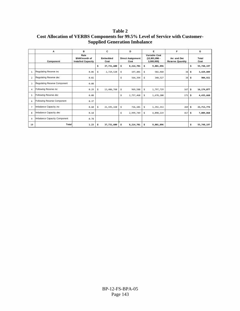
Table 2 Cost Allocation of VERBS Components for 99.5% Level of Service with Customer-

Supplied Generation Imbalance

A B C D E F

Component

Rate $/kW/month of

Installed CapacityEmbedded

CostDirect Assignment

Cost

Variable Cost(12,801,896 - 3,000,000)

Inc and Dec Reserve Quantity

Total Cost

37,731,600$ 8,214,701$ 9,801,896$ 55,748,197$

1 Regulating Reserve inc 0.06 2,729,520$ 197,401$ 502,968$ 34 3,429,889$

2 Regulating Reserve dec 0.02 564,394$ 340,527$ 34 904,921$

3 Regulating Reserve Component 0.08

4 Following Reserve inc 0.29 13,406,760$ 969,588$ 1,797,729$ 167 16,174,077$

5 Following Reserve dec 0.08 2,757,468$ 1,678,200$ 171 4,435,668$

6 Following Reserve Component 0.37

7 Imbalance Capacity inc 0.60 21,595,320$ 726,101$ 1,392,353$ 269 23,713,774$

8 Imbalance Capacity dec 0.18 2,999,749$ 4,090,119$ 417 7,089,868$

9 Imbalance Capacity Component 0.78

10 Total 1.23 37,731,600$ 8,214,701$ 9,801,896$ 55,748,197$

G


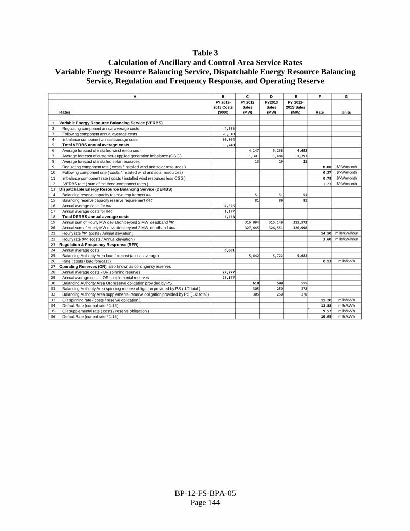
Table 3 Calculation of Ancillary and Control Area Service Rates

Variable Energy Resource Balancing Service, Dispatchable Energy Resource Balancing Service, Regulation and Frequency Response, and Operating Reserve

A B C D E F G

Rates

FY 2012-2013 Costs

($000)

FY 2012 Sales(MW)

FY2013 Sales(MW)

FY 2012-2013 Sales

(MW) Rate Units

1 Variable Energy Resource Balancing Service (VERBS)2 Regulating component annual average costs 4,335

3 Following component annual average costs 20,610

4 Imbalance component annual average costs 30,804

5 Total VERBS annual average costs 55,748

6 Average forecast of installed wind resources 4,147 5,238 4,693

7 Average forecast of customer-supplied generation imbalance (CSGI) 1,301 1,484 1,393

8 Average forecast of installed solar resources 13 29 21

9 Regulating component rate ( costs / installed wind and solar resources ) 0.08 $/kW/month

10 Following component rate ( costs / installed wind and solar resources) 0.37 $/kW/month

11 Imbalance component rate ( costs / installed wind resources less CSGI) 0.78 $/kW/month

12 VERBS rate ( sum of the three component rates ) 1.23 $/kW/month

13 Dispatchable Energy Resource Balancing Service (DERBS)14 Balancing reserve capacity reserve requirement inc 51 51 51

15 Balancing reserve capacity reserve requirement dec 81 80 81

16 Annual average costs for inc 4,576

17 Annual average costs for dec 1,177

18 Total DERBS annual average costs 5,753

19 Annual sum of Hourly MW deviation beyond 2 MW deadband inc 316,004 315,140 315,572

20 Annual sum of Hourly MW deviation beyond 2 MW deadband dec 327,445 326,551 326,998

21 Hourly rate inc (costs / Annual deviation ) 14.50 mills/kW/hour

22 Hourly rate dec (costs / Annual deviation ) 3.60 mills/kW/hour

23 Regulation & Frequency Response (RFR)24 Annual average costs 6,601

25 Balancing Authority Area load forecast (annual average) 5,642 5,722 5,682

26 Rate ( costs / load forecast ) 0.13 mills/kWh

27 Operating Reserves (OR) also known as contingency reserves

28 Annual average costs - OR spinning reserves 27,277

29 Annual average costs - OR supplemental reserves 23,177

30 Balancing Authority Area OR reserve obligation provided by PS 610 500 555

31 Balancing Authority Area spinning reserve obligation provided by PS ( 1/2 total ) 305 250 278

32 Balancing Authority Area supplemental reserve obligation provided by PS ( 1/2 total ) 305 250 278

33 OR spinning rate ( costs / reserve obligation ) 11.20 mills/kWh

34 Default Rate (normal rate * 1.15) 12.88 mills/kWh

35 OR supplemental rate ( costs / reserve obligation ) 9.52 mills/kWh

36 Default Rate (normal rate * 1.15) 10.95 mills/kWh


BONNEVILLE POW ER ADMINISTRATION DOE/BP-4340 • July 2011

GENERATION INPUTS STUDY - BPA.gov - Bonneville ... Determining the Amount of Capacity Provided by...

Documents

Transcript of GENERATION INPUTS STUDY - BPA.gov - Bonneville ... Determining the Amount of Capacity Provided by...