ARTICLE IN PRESS

0098-3004/$ - se

doi:10.1016/j.ca

�Tel.: +1 94

E-mail addr

Computers & Geosciences 34 (2008) 411–421

www.elsevier.com/locate/cageo

Generating and updating multiplicatively weighted Voronoidiagrams for point, line and polygon features in GIS

Pinliang Dong�

Department of Geography, University of North Texas, PO Box 305279, Denton, TX 76203, USA

Received 24 January 2007; received in revised form 23 March 2007; accepted 4 April 2007

Abstract

A Voronoi diagram is an interdisciplinary concept that has been applied to many fields. In geographic information

systems (GIS), existing capabilities for generating Voronoi diagrams normally focus on ordinary (not weighted) point (not

linear or area) features. For better integration of Voronoi diagram models and GIS, a raster-based approach is developed,

and implemented seamlessly as an ArcGIS extension using ArcObjects. In this paper, the methodology and

implementation of the extension are described, and examples are provided for ordinary or weighted point, line, and

polygon features. Advantages and limitations of the extensions are also discussed. The extension has the following

features: (1) it works for point, line, and polygon vector features; (2) it can generate both ordinary and multiplicatively

weighted Voronoi diagrams in vector format; (3) it can assign non-spatial attributes of input features to Voronoi cells

through spatial joining; and (4) it can produce an ordinary or a weighted Euclidean distance raster dataset for spatial

modeling applications. The results can be conveniently combined with other GIS datasets to support both vector-based

spatial analysis and raster-based spatial modeling.

r 2007 Elsevier Ltd. All rights reserved.

Keywords: Spatial analysis; Spatial modeling; Spatial joining; Thiessen polygon; Weighted Euclidean distance

1. Introduction

Given a set of a finite number of distinct points inthe 2-D Euclidean space, a Voronoi diagram of thepoint set is a collection of regions that divideup the plane, and all locations in one region (excepton the region boundary) are closer to the corre-sponding point than to any other point (Fig. 1).Voronoi diagrams are named after the Russianmathematician Georgy Fedoseevich Voronoi whodefined and studied the general n-dimensional case

e front matter r 2007 Elsevier Ltd. All rights reserved

geo.2007.04.005

0 565 2377; fax: +1 940 369 7550.

ess: pdong@unt.edu

in 1908. Discussions on the concept of Voronoidiagram from both historical and geometric view-points can be found in Okabe et al. (1992, 2000).

Voronoi diagrams have been widely appliedto space partition problems in various disciplines,from astronomy to geography to zoology. Okabeet al. (2000) listed 22 fields in which applicationsof Voronoi diagrams can be found, and it isbelieved that the application fields are not limitedto the list. Recent application examples of Voronoidiagrams include Voronoi-based cellular automata(Shi and Pang, 2000), 3-D adaptive tomography ingeophysical prospecting (Bohm et al., 2000), earth-quake distribution analysis and early warning

.

ARTICLE IN PRESS

Fig. 1. A Voronoi diagram of points.

1Takashi Ohyama’s webpage: http://www.nirarebakun.com/

voro/emwvoro.html.2Lomas, T., Create Thiessen Polygons 3.0: http://arcscript.

esri.com.3Tiefelsdorf, M., Boots, B., 1997. GAMBINI Multiplicatively

Weighted Voronoi Diagram. http://info.wlu.ca/%7Ewwwgeog/

facstaff/boots.htm.

P. Dong / Computers & Geosciences 34 (2008) 411–421412

(Nicholson et al., 2000; Cua, 2004; Satriano et al.,2006), exposure analysis of wireless sensor network(Meguerdichian et al., 2001), reservoir modeling inpetroleum exploitation (Subbeya et al., 2004),environmental risk assessment (Greco et al., 2005),remote sensing mapping accuracy assessment(Nelson et al., 2005), biological structure character-ization (Costa et al., 2006), and domain boundaryreconstruction for point datasets (Kolingerovaand Zalik, 2006). In geophysics, Iervolino et al.(2006) discussed real-time risk analysis for earth-quake early warning where magnitude estimationis performed via the Bayesian approach, andthe earthquake localization is based on theVoronoi cells. In geography, some of the earlyapplications of Voronoi diagrams in market areaanalysis can be dated back to 1841 (Shieh, 1985;Okabe et al., 2000). Later examples includeBoots (1980, 1986) and Boots and Getis (1988),among many others. Economic geography andurban geography problems are major applicationareas of Voronoi diagrams in geography, forexample, modeling retail trade areas (Boots andSouth, 1997) and solving locational optimizationproblems (Okabe et al., 1992, 2000; Okabeand Suzuki, 1997). Since the 1990s, Voronoidiagram has received increased attention as aspatial data model in GIS (Gold, 1991, 1994,2004; Okabe et al., 1994; Gold and Condal, 1995;Anton et al., 1998; Li et al., 1999; Chakroun et al.,2000; Chen et al., 2001; Boots et al., 2003; Gold andAngel, 2006; Ledoux and Gold, 2006; Masuyama,2006).

Although theoretical and computational aspectsof Voronoi diagrams have been extensively docu-mented, limited efforts have been made to bringVoronoi diagrams into GIS for practical use. Thereare 2 major issues concerning the integration ofVoronoi diagrams and GIS: (1) many approaches to

generating Voronoi diagrams have worked withpoint data outside GIS, and it is not straightforwardto bring the results into GIS (for example, Reitsmaet al., 2004; Ohyama1); (2) in many applications,the location of a feature alone is not enough, andthe importance (or weight) of the feature shouldbe taken into account. Many existing methods inGIS have focused on ordinary point features, butnot weighted features including points, line seg-ments, and polygons. Examples of these issuescan be found in literature and from GIS softwareproducts. Lomas2 created a Thiessen PolygonDynamic Link Library (DLL) for the ArcGISsoftware developed by the Environmental SystemsResearch Institute (ESRI), to generate Voronoipolygons. But the DLL only works for point data,and weights are not taken into account. In ArcGIS9.1 released by ESRI in 2005, ordinary Voronoidiagrams (OVDs) can be generated in rasterformat using the Euclidean Allocation tool in theSpatial Analyst extension, or displayed in vectorformat using the Geostatistical Analyst extension,or created from a ‘‘store layer’’ (point dataset) in theBusiness Analyst extension. However, none of theextensions can create weighted Voronoi diagrams.Several references are noteworthy in bringingweighted Voronoi diagrams into GIS. Tiefelsdorfand Boots3 developed a program GAMBINI whichcalculates, draws and exports multiplicativelyweighted Voronoi diagrams on Windows 3.1 andWindows 95/NT. GAMBINI is loosely linked toGIS via input and output files, and Voronoipolygons need to be manually created from theimported arcs, which can be a time-consumingprocess. Using vector data structure and algorithms,Gahegan and Lee (2000) studied 6 specific Voronoidiagram variants, including multiplicativelyweighted Vironoi diagrams, to support interactivespatial analysis. They concluded that, comparedwith OVDs, the weighting of generator pointsallows for modeling a wide range of situations,but the reconstruction algorithm is more complex.Mu (2004) demonstrated the composition anddecomposition of multiplicatively weighted Voronoipolygons, and proposed using decomposition to

ARTICLE IN PRESS

Fig. 2. Distance surfaces for (A) wa ¼ wb; (B) wa4wb; and

(C) waowb.

P. Dong / Computers & Geosciences 34 (2008) 411–421 413

understand landscape processes. It seems that allthese references on weighted Voronoi diagrams inGIS are for point generators, and the methods forgenerating Voronoi diagrams are all vector-based.In fact, as reviewed by Li et al. (1999), vector-basedmethods for generating Voronoi diagrams workwell for point datasets, but are not efficient for linesegments and area features. In addition to pointfeatures, it is desirable to generate Voronoi dia-grams for line segments and area features to supportcertain applications. Okabe and Suzuki (1997)noticed that the locational optimization problemsof line-like and area-like facilities are less developedand worth challenging. In geosciences, weightedVoronoi diagrams for line segments and areafeatures can be very useful in some applications.For example, the zone of influence for active faultsmay be assessed based on the length of the faultsegments, and target areas in mineral explorationcan be delineated depending on the size of alterationzones.

For better integration of Voronoi diagrams andGIS to support various applications, it is importantto bridge the gap between the above-mentionedissues. The objective of this research is to develop araster-based approach to generating and updatingboth ordinary and multiplicatively weightedVoronoi diagrams for point, line, and polygonfeatures in a GIS environment. Implementedas an ArcGIS extension, the approach acceptspoint, line, and polygon features in shapefilevector format, calculates ordinary or weightedEuclidean distances in a raster environment, andfinally creates an output Voronoi diagram as apolygon shapefile and an ordinary or weighteddistance raster. Optionally, non-spatial attributesof input features can be assigned to outputVoronoi diagrams through spatial joining. There-fore, the output from the extension can be usedfor both vector-based spatial analysis and raster-based spatial modeling. The major reason foremploying the raster-based approach is that point,line, and polygon features can be treated in the samemanner when calculating distance rasters usingArcObjects, which greatly simplifies the processfor generating Voronoi diagrams. Following thisintroduction, Section 2 describes the methodologyand implementation of the extension, Section 3provides examples for generating and updatingordinary and weighted Voronoi diagrams, followedby discussions in Section 4, and conclusion inSection 5.

2. Methodology and implementation

2.1. Generating multiplicatively weighted Voronoi

diagrams

In Fig. 1, it is assumed that each generator pointhas the same weight. In many spatial analysis andmodeling problems, generators have differentweights due to the differences in their properties.For example, earthquakes have different magni-tudes, and cities have different population sizes.Okabe et al. (2000) discussed 4 types of weightedVoronoi diagrams: multiplicatively weighted, addi-tively weighted, compoundly weighted, and powerdiagram. This study focuses on multiplicativelyweighted Voronoi diagrams.

Given 2 generators A and B with weights wa andwb (wa40, wb40), respectively, we can describe theEuclidean distances to A and B using 2 upside-downright circular cones (Fig. 2), as if 2 trees A and B arecompeting with each other for canopy space. Inorder to show the Euclidean distance from everypoint location to a generator, we use a raster datamodel to represent distance values. Therefore,each cone represents the distance raster surface forthe generator. The 2 cones touch each other at Q.

ARTICLE IN PRESS

Fig. 3. Relationship between ordinary Euclidean distance (OED)

and weighted Euclidean distance (WED).

Fig. 4. Weighted Euclidean distance (WED) raster surfaces for 3

generators.

P. Dong / Computers & Geosciences 34 (2008) 411–421414

For simplicity, let the raster cell value at point Q beequal to unit length 1 (PQ ¼ 1). If wa ¼ wb, the 2rasters represent ‘‘ordinary Euclidean distance(OED)’’ (Fig. 2A). Otherwise, they represent‘‘weighted Euclidean distance (WED)’’ (Fig. 2B, C).

What is the relationship between OED and WEDfor the generator point A? This can be answered byanalyzing Fig. 3, a composite of the triangle ABQ inFig. 2A and the triangle ABQ in Fig. 2B. For arandom point F between A and B (Fig. 3), FH isOED, FG is WED, and FH ¼ AF . Since A and Bare multiplicatively weighted generators, AP shouldbe proportionally related to wa, that is, AP ¼ cwa

(c40). Obviously, we have

tan a ¼PQ

AP¼

FG

AF. (1)

From (1) we have:

FG ¼PQ � AF

AP¼

FH

cwa

. (2)

Because c is a constant, Eq. (2) can be simplifiedto

FG ¼FH

wa

. (3)

Eq. (3) shows that WED for generator A can becalculated using OED divided by the weight wa.Denote g(x, y) as the WED raster, and f(x, y) as theOED raster, Eq. (3) can be expressed as

gðx; yÞ ¼f ðx; yÞ

wa

ðwa40Þ. (4)

Similar expressions can be obtained for generatorB. Fig. 4 illustrates a WED raster surface profile for3 generators A, B, and C with weights wa, wb, andwc, respectively, and wb4wa4wc. The shadedportions in Fig. 4 represent the final WED rastersurface profile after all generators are taken intoaccount. From Fig. 4 it can be seen that the finalWED raster, R(x, y), can be obtained by calculating

cell-by-cell minimum of the WED rasters obtainedfrom all generators:

Rðx; yÞ ¼ min½giðx; yÞ� ði ¼ 0; 1; 2; . . . ; k � 1Þ, (5)

where x and y are individual cell locations, and k isthe total number of generators. It should be notedthat the min function in Eq. (5) works on the cell-by-cell basis where x ¼ 0, 1, 2,y,m�1 and y ¼ 0,1, 2,y n�1 (m is the number of columns and n isthe number of rows in a raster). In actualimplementation, it may not be feasible to store k

rasters in memory in order to calculate R(x, y),especially if a large number of features are involvedfor generating Voronoi diagrams. This problem canbe solved by comparing the distance rasters in aloop structure throughout all features (generators),as described in the following pseudo-code:

k – The number of features.i – Feature index.r0(x, y) – The 1st raster for ordinary Euclideandistance.s0(x, y) – The 1st raster for weighted Euclideandistance.r1(x, y) – The subsequent rasters for ordinaryEuclidean distance.s1(x, y) – The subsequent rasters for weightedEuclidean distance.t(x, y) – The temporary raster for cell-by-cellminimum of two distance rasters.v(x, y) – The final raster for cell-by-cell minimum ofall distance rasters.wi – The constant raster representing the weightvalue for feature i.

For i ¼ 0 to k�1If i ¼ 0 Then

Calculate r0(x, y)s0(x, y) ¼ r0(x, y)/wi

v(x, y) ¼ s0(x, y)Else

Calculate r1(x, y)

ARTICLE IN PRESSP. Dong / Computers & Geosciences 34 (2008) 411–421 415

s1(x, y) ¼ r1(x, y)/wi

t(x, y) ¼Minimum[v(x, y), s1(x, y)]v(x, y) ¼ t(x, y)

EndIfNext i

It can be seen from the pseudo-code that only 7rasters are required at any time, no matter howmany features are involved in generating theweighted Voronoi diagram. The raster objects canbe set to ‘‘Nothing’’ at the end of the process to freememory.

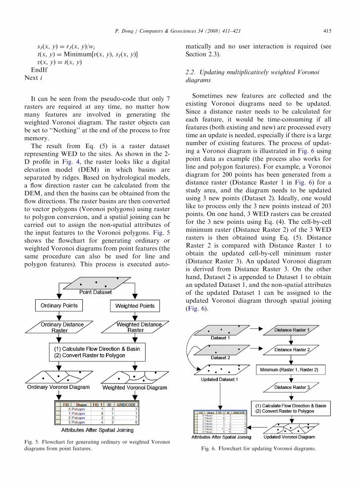
The result from Eq. (5) is a raster datasetrepresenting WED to the sites. As shown in the 2-D profile in Fig. 4, the raster looks like a digitalelevation model (DEM) in which basins areseparated by ridges. Based on hydrological models,a flow direction raster can be calculated from theDEM, and then the basins can be obtained from theflow directions. The raster basins are then convertedto vector polygons (Voronoi polygons) using rasterto polygon conversion, and a spatial joining can becarried out to assign the non-spatial attributes ofthe input features to the Voronoi polygons. Fig. 5shows the flowchart for generating ordinary orweighted Voronoi diagrams from point features (thesame procedure can also be used for line andpolygon features). This process is executed auto-

Fig. 5. Flowchart for generating ordinary or weighted Voronoi

diagrams from point features.

matically and no user interaction is required (seeSection 2.3).

2.2. Updating multiplicatively weighted Voronoi

diagrams

Sometimes new features are collected and theexisting Voronoi diagrams need to be updated.Since a distance raster needs to be calculated foreach feature, it would be time-consuming if allfeatures (both existing and new) are processed everytime an update is needed, especially if there is a largenumber of existing features. The process of updat-ing a Voronoi diagram is illustrated in Fig. 6 usingpoint data as example (the process also works forline and polygon features). For example, a Voronoidiagram for 200 points has been generated from adistance raster (Distance Raster 1 in Fig. 6) for astudy area, and the diagram needs to be updatedusing 3 new points (Dataset 2). Ideally, one wouldlike to process only the 3 new points instead of 203points. On one hand, 3 WED rasters can be createdfor the 3 new points using Eq. (4). The cell-by-cellminimum raster (Distance Raster 2) of the 3 WEDrasters is then obtained using Eq. (5). DistanceRaster 2 is compared with Distance Raster 1 toobtain the updated cell-by-cell minimum raster(Distance Raster 3). An updated Voronoi diagramis derived from Distance Raster 3. On the otherhand, Dataset 2 is appended to Dataset 1 to obtainan updated Dataset 1, and the non-spatial attributesof the updated Dataset 1 can be assigned to theupdated Voronoi diagram through spatial joining(Fig. 6).

Fig. 6. Flowchart for updating Voronoi diagrams.

ARTICLE IN PRESSP. Dong / Computers & Geosciences 34 (2008) 411–421416

It should be noted that the above updatingprocess can only update features within the extent(bounding-box or envelope) of existing features.Any new feature that is outside the existing extentwill be ignored. If the extent of the new features isnot completely contained by the existing extent, theprogram will generate a warning message. In thatcase, it is recommended to append the new featuresto existing features, and then generate new Voronoidiagrams as described in Section 2.1.

2.3. Implementation with ArcObjects

Written in C++, ESRI’s ArcObjects are plat-form-independent software components for GISapplication development. Several choices of custo-mization are available for developers and users toadd new GIS functionality to ArcGIS. Among thechoices, extensions provide the developer with a

Table 1

Components of visual basic ActiveX DLL project for weighted

Voronoi diagram extension

Forms frmVoronoi.frm

Modules FunctionModules.bas

Class modules Extension.cls (Implements: IExtension,

IExtensionConfig)

Help.cls (Implements: ICommand)

StartVoronoi.cls (Implements: ICommand)

Toolbar.cls (Implements: IToolbarDef)

Related

documents

Voronoi.res (resource file)

Fig. 7. Graphical user interface. (A)

powerful mechanism for extending the core func-tionality of ArcGIS applications. An extension canprovide new tools on a toolbar, listen for andrespond to events, and perform many other GIStasks. The weighted Voronoi diagram extension wasdeveloped using Microsoft Visual Basic 6.0 andESRI’s ArcObjects 9.1. From a Visual BasicActiveX Dynamic Link Library (DLL) project, aDLL file was compiled. The DLL file can bedeployed to a user’s computer with other relevantfiles. Table 1 lists the components of the DLLproject and major interfaces. The IExtension inter-face defines the name of the extension and specifieswhat action takes place when the extension isstarted or shut down. The IExtensionConfig inter-face specifies the state of the extension, and providesthe name and description of the extension in theExtension dialog box.

The graphical user interface has 2 tabs: Generate(Fig. 7A) and Update (Fig. 7B). Using the Generatetab, the user can generate ordinary or weightedVoronoi diagrams from point, line, or polygonfeatures. A raster showing OED or WED (if weightsare used) is generated, as well as a Voronoi polygonshapefile. Non-spatial attributes from input featurescan be transferred to Voronoi polygons automati-cally through spatial joining. Once a distance rasteris generated, the user can use new features to updatethe distance raster and create updated Voronoipolygons (Fig. 7B). The output Voronoi diagrams(shapefiles) and distance raster datasets can be usedin spatial analysis and modeling for various

Generate tab; (B) Update tab.

ARTICLE IN PRESSP. Dong / Computers & Geosciences 34 (2008) 411–421 417

applications. Examples of generating and updatingordinary and weighted Voronoi diagrams areprovided in the next section. More examples andinformation on the functionality can be found inthe user’s guide. The free extension and relevantdocuments are available from the author.

3. Examples

3.1. Generating weighted Voronoi diagrams

In Fig. 8, the left side (Fig. 8A, C, E) shows theoriginal data points and generated Voronoi dia-grams. The numbers show the weight of thepoints. The right side of Fig. 8 shows WED rasters(Fig. 8B, D, F). In Fig. 8A, all the points have aweight 1, and the resulting Voronoi diagram isan OVD in which polygon sides are straight linesegments. In fact, from Eq. (4) it is not difficult toprove that an OVD can be generated using aconstant weight (not necessarily 1) for all features.

Fig. 8. Examples of weighted Voronoi diagram

Fig. 8C and E show that weighted Voronoidiagrams will be created if the weights are different.Since these are multiplicatively weighted Voronoidiagrams, the weight ratio for 2 adjacent points isequal to the ratio of the distances from the points tothe Voronoi boundary between them. For example,if we draw a line connecting the point with weight0.8 with the point with weight 1.6 in Fig. 8E, we cansee that the line is divided by the polygon boundarywith a 1/2 ratio.

Fig. 9 shows a composite display of 10 linesegments, their Voronoi diagrams, and the distancerasters. Fig. 9A is an OVD. In Fig. 9B, the lengthfield of the line attribute table was used as weightfield to create a weighted Voronoi diagram.Compared with Fig. 8A, it can be seen that shorterline segments in Fig. 9B have smaller Voronoipolygons.

Similar to Fig. 9, Fig. 10 shows a compositedisplay of 10 polygons, their Voronoi diagrams, andthe distance rasters. Fig. 10A is an OVD, and

s and distance rasters for point features.

ARTICLE IN PRESS

Fig. 9. Voronoi diagrams for lines. (A) Ordinary Voronoi diagram; (B) weighted Voronoi diagram using line length as weight.

Fig. 10. Voronoi diagrams for polygons. (A) Ordinary Voronoi diagram; (B) weighted Voronoi diagram using polygon area as weight.

Fig. 11. Updating Voronoi diagrams. (A) and (C) show original points (dot symbols), new points (cross symbols), and updated Voronoi

diagrams; (B) and (D) are weighted distance rasters.

P. Dong / Computers & Geosciences 34 (2008) 411–421418

Fig. 9B is a weighted Voronoi diagram using featurearea as weight. Compared with Fig. 9A, it can beseen that smaller polygons in Fig. 9B have smallerVoronoi polygons.

3.2. Updating weighted Voronoi diagrams

The following examples show how the weightedVoronoi diagram in Fig. 8E can be updated by 3

ARTICLE IN PRESSP. Dong / Computers & Geosciences 34 (2008) 411–421 419

additional points. This process requires the originalpoints (dots in Fig. 8E) and the original weighteddistance raster (Fig. 8F). Three new pointswith weights 0.9, 1.4, and 1.5 (x symbols inFig. 11A) are appended to the original pointsto create a new Voronoi diagram (polygons inFig. 11A). The updated weighted distance rasteris shown in Fig. 11B. Fig. 11C and D show theupdated weighted Voronoi diagram and weighteddistance raster when the 3 new points (x symbols inFig. 11C) are added to 3 different locations.

4. Discussions

Some advantages and limitations of the extensionshould be discussed. The advantages are as follows:

(1)

Fig.

nega

it works seamlessly with ArcGIS, and it canhandle point, line, and polygon features;

(2)

it can generate both ordinary and multiplica-tively weighted Voronoi diagrams. The weightsfor multiplicatively weighted Voronoi diagramscan be from an existing numeric field in theattribute table, or from a new numeric field withuser-specified values;

(3)

the input non-spatial attributes can be auto-matically assigned to output Voronoi polygonsthrough spatial joining;

(4)

Voronoi diagrams generated by this extensioncan be conveniently updated by inserting addi-tional generators (points, lines, or polygons);and

(5)

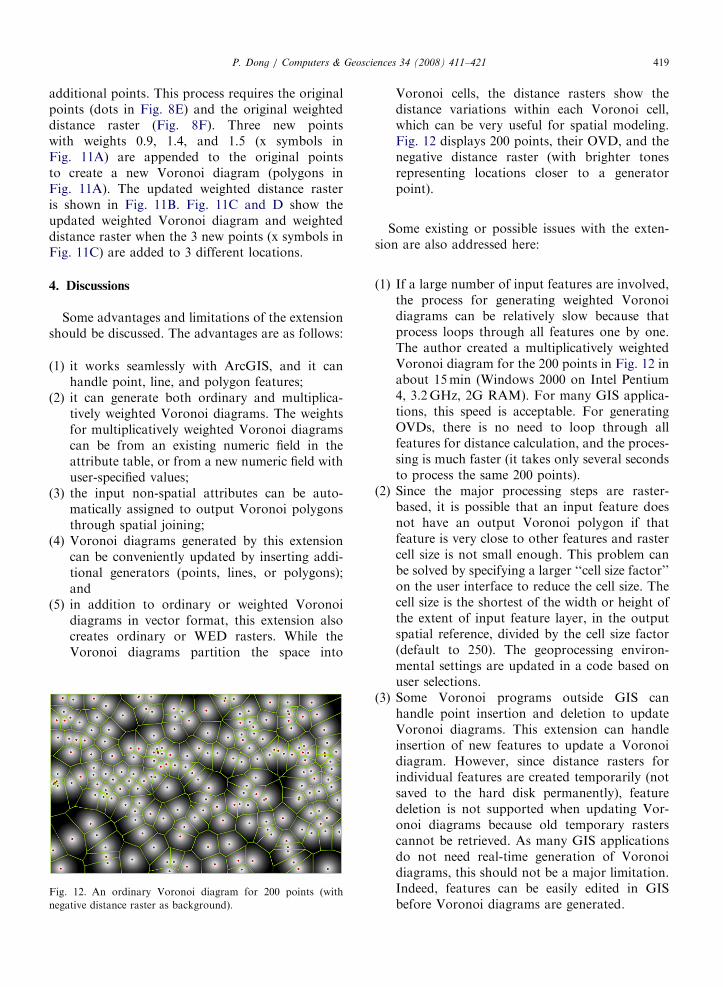
in addition to ordinary or weighted Voronoidiagrams in vector format, this extension alsocreates ordinary or WED rasters. While theVoronoi diagrams partition the space into

12. An ordinary Voronoi diagram for 200 points (with

tive distance raster as background).

Voronoi cells, the distance rasters show thedistance variations within each Voronoi cell,which can be very useful for spatial modeling.Fig. 12 displays 200 points, their OVD, and thenegative distance raster (with brighter tonesrepresenting locations closer to a generatorpoint).

Some existing or possible issues with the exten-sion are also addressed here:

(1)

If a large number of input features are involved,the process for generating weighted Voronoidiagrams can be relatively slow because thatprocess loops through all features one by one.The author created a multiplicatively weightedVoronoi diagram for the 200 points in Fig. 12 inabout 15min (Windows 2000 on Intel Pentium4, 3.2GHz, 2G RAM). For many GIS applica-tions, this speed is acceptable. For generatingOVDs, there is no need to loop through allfeatures for distance calculation, and the proces-sing is much faster (it takes only several secondsto process the same 200 points).

(2)

Since the major processing steps are raster-based, it is possible that an input feature doesnot have an output Voronoi polygon if thatfeature is very close to other features and rastercell size is not small enough. This problem canbe solved by specifying a larger ‘‘cell size factor’’on the user interface to reduce the cell size. Thecell size is the shortest of the width or height ofthe extent of input feature layer, in the outputspatial reference, divided by the cell size factor(default to 250). The geoprocessing environ-mental settings are updated in a code based onuser selections.

(3)

Some Voronoi programs outside GIS canhandle point insertion and deletion to updateVoronoi diagrams. This extension can handleinsertion of new features to update a Voronoidiagram. However, since distance rasters forindividual features are created temporarily (notsaved to the hard disk permanently), featuredeletion is not supported when updating Vor-onoi diagrams because old temporary rasterscannot be retrieved. As many GIS applicationsdo not need real-time generation of Voronoidiagrams, this should not be a major limitation.Indeed, features can be easily edited in GISbefore Voronoi diagrams are generated.

ARTICLE IN PRESSP. Dong / Computers & Geosciences 34 (2008) 411–421420

It should be noted that the references in thispaper and the topic of this paper are all on planarVoronoi diagrams generated from Euclidean dis-tance. As a side note, it is fascinating to see thatOVDs have been generated for networks using theshortest-path distance, as demonstrated in thesoftware SANET developed by Okabe et al.4 Futureversions of SANET will be able to create weightedVoronoi diagrams for networks (Okabe, 2007,personal communication).

5. Conclusion

A raster-based approach to generating andupdating ordinary and multiplicatively weightedVoronoi diagrams is developed and implemented asan extension in ArcGIS. It works seamlessly withArcGIS, and can handle point, line, and polygonfeatures. It can perform spatial joining to link inputfeatures and output Voronoi polygons. In additionto Voronoi diagrams in vector format, the extensionalso creates ordinary or WED rasters. The Voronoidiagrams and distance rasters can be convenientlycombined with other GIS datasets to support bothvector-based spatial analysis and raster-based spa-tial modeling. The analyses of the advantages andlimitations of the extension suggest that it can meetthe requirements of many GIS applications, andthat it can significantly improve the integration ofVoronoi diagram models and GIS applications.

Acknowledgments

The author would like to thank two anonymousreviewers who provided valuable comments thatimproved this paper.

References

Anton, F., Mioc, D., Gold, C.M., 1998. Dynamic additively

weighted Voronoi diagrams made easy. In: Proceedings of the

Tenth Canadian Conference on Computational Geometry

(CCCG’98), Montreal, Canada, p. 2.

Bohm, G., Galuppo, P., Vesnaver, A., 2000. 3D adaptive

tomography using Delaunay triangles and Voronoi polygons.

Geophysical Prospecting 48, 723–744.

Boots, B.N., 1980. Weighting Thiessen polygons. Economic

Geography 56, 248–259.

Boots, B.N., 1986. Voronoi (Thiessen) Polygons. Geo Books,

Norwich, UK, 51pp.

4Okabe’s web page: http://ua.t.u-tokyo.ac.jp/okabelab/atsu.

Boots, B.N., Getis, A., 1988. Point Pattern Analysis. Sage

Publications, Newbury Park, CA, 93pp.

Boots, B., South, R., 1997. Modeling retail trade areas using

higher-order, multiplicatively weighted Voronoi diagrams.

Journal of Retailing 73, 519–536.

Boots, B., Okabe, A., Thomas, R. (Eds.), 2003. Modelling

Geographical Systems: Statistical and Computational

Applications. Kluwer Academic Publishers, Dordrecht, The

Netherlands, 356pp.

Chakroun, H., Benie, G., O’Neill, N.T., Desilets, J., 2000. Spatial

analysis weighting algorithm using Voronoi diagrams. Inter-

national Journal of Geographical Information Science 14,

319–336.

Chen, J., Li, C., Li, Z., Gold, C., 2001. A Voronoi-based

9-intersection model for spatial relations. Interna-

tional Journal of Geographical Information Science 15,

201–220.

Costa, L., Rocha, F., Lima, S., 2006. Characterizing polygonality

in biological structures. Physical Review E 73, 1–8.

Cua, G.B., 2004. Creating the virtual seismologist: developments

in ground motion characterization and seismic early warning.

Unpublished Ph.D. Dissertation, California Institute of

Technology, Pasadena, California, 408pp.

Gahegan, M., Lee, I., 2000. Data structures and algorithms to

support interactive spatial analysis using dynamic Voronoi

diagrams. Computers, Environment and Urban Systems 24,

509–537.

Gold, C.M., 1991. Problems with handling spatial data—the

Voronoi approach. CISM (Canadian Institute of Surveying

and Mapping) Journal 45, 65–80.

Gold, C.M., 1994. A review of potential applications of Voronoi

methods in geomatics. In: Proceedings of the Canadian

Conference on GIS, Ottawa, Canada, pp. 1647–1656.

Gold, C.M., 2004. Applications of kinetic Voronoi diagrams.

In: Proceedings of the Third Voronoi Conference on

Analytic Number Theory and Space Tilings, Kiev, Ukraine,

pp. 169–178.

Gold, C.M., Angel, P., 2006. Voronoi hierarchies. In: Proceed-

ings of GIScience, Munster, Germany, pp. 99–111.

Gold, C.M., Condal, A.R., 1995. A spatial data structure

integrating GIS and simulation in a marine environment.

Marine Geodesy 18, 213–228.

Greco, F., Lawson, A.B., Cocchi, D., Temples, T., 2005. Some

interpolation estimators in environmental risk assessment for

spatially misaligned health data. Environmental and Ecolo-

gical Statistics 12, 379–395.

Iervolino, I., Convertito, V., Giorgio, M., Manfred, G., Zollo, A.,

2006. Real-time hazard analysis for earthquake early warning.

In: Proceedings of the First European Conference on Earth-

quake Engineering and Seismology, Geneva, Switzerland,

Paper no. 850.

Kolingerova, I., Zalik, B., 2006. Reconstructing domain bound-

aries within a given set of points, using Delaunay triangula-

tion. Computers & Geosciences 32, 1310–1319.

Ledoux, H., Gold, C.M., 2006. A Voronoi-based map algebra.

In: Reidl, A., Kainz, W., Elmes, G. (Eds.), Progress in Spatial

Data Handling—12th International Symposium on Spatial

Data Handling. Springer, New York, pp. 117–131.

Li, C., Chen, J., Li., Z., 1999. A raster-based method for

computing Voronoi diagrams of spatial objects using dynamic

distance transformation. International Journal of Geographi-

cal Information Science 13, 209–225.

ARTICLE IN PRESSP. Dong / Computers & Geosciences 34 (2008) 411–421 421

Masuyama, A., 2006. Methods for detecting apparent differences

between spatial tessellations at different time points. Interna-

tional Journal of Geographical Information Science 20,

633–648.

Meguerdichian, S., Koushanfar, F., Qu, G., Potkonjak, M., 2001.

Exposure in wireless Ad-Hoc sensor networks. In: Proceedings

of the Seventh Annual International Conference on Mobile

Computing and Networking, Rome, Italy, pp. 139–150.

Mu, L., 2004. Polygon characterization with the multiplicatively

weighted Voronoi diagram. The Professional Geographer 56,

223–239.

Nelson, T., Boots, B., Wulder, M.A., 2005. Techniques for

accuracy assessment of tree locations extracted from remotely

sensed imagery. Journal of Environmental Management 74,

265–271.

Nicholson, T., Sambridge, M., Gudmundsson, O., 2000. On

entropy and clustering in earthquake hypocenter distribu-

tions. Geophysical Journal International 142, 37–51.

Okabe, A., Suzuki, A., 1997. Locational optimization problems

solved through Voronoi diagrams. European Journal of

Operational Research 98, 445–456.

Okabe, A., Boots, B., Sugihara, K., 1992. Spatial Tessellations—

Concepts and Applications of Voronoi Diagrams. Wiley,

Chichester, UK, 532pp.

Okabe, A., Boots, B., Sugihara, K., 1994. Nearest neighbourhood

operations with generalized Voronoi diagrams: a review.

International Journal of Geographical Information Systems

8, 43–71, 403.

Okabe, A., Boots, B., Sugihara, K., Chiu, S.N., 2000. Spatial

Tessellations: Concepts and Applications of Voronoi Diagrams,

second ed. Wiley, Chichester, UK, 671pp.

Reitsma, R., Trubin, S., Sethia, S., 2004. Information space

regionalization using adaptive multiplicatively weighted

Voronoi diagrams. In: Proceedings of the Eighth Interna-

tional Conference on Information Visualisation, London,

UK, pp. 290–294.

Satriano, C., Lomax, A., Zollo, A., 2006. Optimal, real-time

earthquake location for early warning. Geophysical Research

Abstracts 8, 08883.

Shi, W., Pang, M.Y.C., 2000. Development of Voronoi-based

cellular automata—an integrated dynamic model for geo-

graphic information systems. International Journal of

Geographical Information Science 14, 455–474.

Shieh, Y.-N., 1985. K.H. Rau and the economic law of market

areas. Journal of Regional Science 25, 191–199.

Subbeya, S., Christiea, M., Sambridge, M., 2004. Prediction

under uncertainty in reservoir modeling. Journal of Petroleum

Science and Engineering 44, 143–153.