Generating an aerodynamic model for projectile flight...
24
Generating an aerodynamic model for projectile flight simulation using unsteady time accurate computational fluid dynamic results J. Kokes 1 , M. Costello 2 & J. Sahu 3 1 Orbital Sciences Corporation, USA 2 Georgia Institute of Technology, USA 3 U.S. Army Research Laboratory, USA Abstract A method to efficiently generate a complete aerodynamic description for projectile flight dynamic modeling is described. At the core of the method is an unsteady, time accurate computational fluid dynamics simulation that is tightly coupled to a rigid body dynamics simulation. A set of n short time snippets of simulated projectile motion at m different Mach numbers is computed and employed as baseline data. For each time snippet, aerodynamic forces and moments and the full rigid body state vector of the projectile are known. With time synchronized air loads and state vector information, aerodynamic coefficients can be estimated with a simple fitting procedure. By inspecting the condition number of the fitting matrix, it is straight forward to assess the suitability of the time history data to predict a selected set of aerodynamic coefficients. To highlight the merits of this technique it is exercised on example data for a fin stabilized projectile. The technique is further exercised for a fin and spin stabilized projectile using simulated data from a standard trajectory code. Keywords: projectile, flight dynamics, aerodynamic coefficients, CFD. 1 Introduction There are roughly four classes of techniques to predict aerodynamic forces and moments on a projectile in atmospheric flight: empirical methods, wind tunnel testing, computational fluid dynamics simulation, and spark range testing. Empirical techniques aerodynamically describe the projectile with a set of © 2007 WIT Press WIT Transactions on Modelling and Simulation, Vol 45, www.witpress.com, ISSN 1743-355X (on-line) Computational Ballistics III 31 doi:10.2495/CBAL070041
Transcript of Generating an aerodynamic model for projectile flight...
Generating an aerodynamic model for projectile flight simulation using unsteady time accurate computational fluid dynamic results
J. Kokes1, M. Costello2 & J. Sahu3 1Orbital Sciences Corporation, USA 2Georgia Institute of Technology, USA 3U.S. Army Research Laboratory, USA
Abstract
A method to efficiently generate a complete aerodynamic description for projectile flight dynamic modeling is described. At the core of the method is an unsteady, time accurate computational fluid dynamics simulation that is tightly coupled to a rigid body dynamics simulation. A set of n short time snippets of simulated projectile motion at m different Mach numbers is computed and employed as baseline data. For each time snippet, aerodynamic forces and moments and the full rigid body state vector of the projectile are known. With time synchronized air loads and state vector information, aerodynamic coefficients can be estimated with a simple fitting procedure. By inspecting the condition number of the fitting matrix, it is straight forward to assess the suitability of the time history data to predict a selected set of aerodynamic coefficients. To highlight the merits of this technique it is exercised on example data for a fin stabilized projectile. The technique is further exercised for a fin and spin stabilized projectile using simulated data from a standard trajectory code. Keywords: projectile, flight dynamics, aerodynamic coefficients, CFD.
1 Introduction
There are roughly four classes of techniques to predict aerodynamic forces and moments on a projectile in atmospheric flight: empirical methods, wind tunnel testing, computational fluid dynamics simulation, and spark range testing. Empirical techniques aerodynamically describe the projectile with a set of
© 2007 WIT PressWIT Transactions on Modelling and Simulation, Vol 45, www.witpress.com, ISSN 1743-355X (on-line)
Computational Ballistics III 31
doi:10.2495/CBAL070041
geometric properties (diameter, number of fins, nose type, nose radius, etc) and catalog aerodynamic coefficients of many different projectiles as a function of these features. The database of aerodynamic coefficients as a function of projectile features is typically obtained from wind tunnel or spark range tests. This data is fit to multivariable equations to create generic models for aerodynamic coefficients as a function of these basic projectile geometric properties. Examples of this approach to projectile aerodynamic coefficient estimation include Missile DATCOM, PRODAS, and AP98 [1–6]. The advantage of this technique is that it is a general method applicable to any projectile. However, it is the least accurate method of the four methods mentioned above, particularly for new configurations that fall outside the realm of projectiles used to form the basic aerodynamic database. The empirical method has been found very useful in conceptual design of projectiles where rapid and inexpensive estimates of aerodynamic coefficients are needed. In wind tunnel testing, a specific projectile is mounted in a wind tunnel at various angles of attack with aerodynamic forces and moments measured at various Mach numbers using a sting balance. Wind tunnel testing has the obvious advantage of being based on direct measurement of aerodynamic forces and moments on the projectile. It is also relatively easy to change the wind tunnel model to allow detailed parametric effects to be investigated. The main disadvantage to wind tunnel testing is that it requires a wind tunnel and as such is modestly expensive. Furthermore, dynamic derivatives such as pitch and roll damping as well as Magnus force and moment coefficients are difficult to obtain in a wind tunnel and require a complex physical wind tunnel model. Wind tunnel testing is often used during projectile development programs to converge on fine details of the aerodynamic design of the shell [7,8]. In computational fluid dynamics (CFD) simulation, the fundamental fluid dynamic equations are numerically solved for a specific configuration. The most sophisticated computer codes are capable of unsteady time accurate computations using the Navier–Stokes equations. Examples of these tools include, for example, CFD++, Fluent, and Overflow-D. Over the past couple of decades, tremendous strides have been made in the application of CFD to prediction of aerodynamic loads on air vehicles, including projectiles. CFD is based on first principles and does not involve physical testing. It is a general method that is valid for any projectile configuration. However, CFD is computationally expensive and requires powerful computers to obtain results in a reasonably timely manner [9–22]. In spark range aerodynamic testing, a projectile is fired through an enclosed building. At a discrete number of points during the flight of the projectile (< 30) the state of the projectile is measured using spark shadowgraphs [23–27]. The projectile state data is subsequently fit to a rigid 6 degree-of-freedom projectile model using the aerodynamic coefficients as the fitting parameters [28–30]. Spark range aerodynamic testing is considered the gold standard for projectile aerodynamic coefficient estimation. It is the most accurate method for obtaining aerodynamic data on a specific projectile configuration. It usually the most expensive alternative, requires a spark range facility, and strictly speaking is only valid for the specific projectile configuration tested.
© 2007 WIT PressWIT Transactions on Modelling and Simulation, Vol 45, www.witpress.com, ISSN 1743-355X (on-line)
32 Computational Ballistics III
Various researchers have used CFD to estimate aerodynamic coefficient estimation of projectiles. Early work focused on Euler solvers applied to steady flow problems while more recent work has solved the Reynolds averaged Navier–Stokes equations and Large Eddy Simulation Navier Stokes equations for both steady and unsteady conditions [9–22]. For example, to predict pitch damping Weinacht prescribed projectile motion to mimic a typical pitch damping wind tunnel test in a CFD simulation to estimate the different components of the pitch damping coefficient of a fin stabilized projectile [31]. Excellent agreement between computed and measured pitch damping was attained. Algorithm and computing advances have also led to coupling of CFD codes to projectile rigid body dynamics codes for simulation of free flight motion of a projectile in a time accurate manner. Aerodynamic forces and moments are computed with the computational fluid dynamics solver while the free flight motion of the projectile is computed by integrating the rigid body dynamic (RBD) equations of motion. The ability to simulate the flight of a projectile using first principles has led to the notion of “virtual fly outs” where the simulation tools above are used to replicate a spark range test. Along these lines, Sahu achieved excellent agreement between spark range measurements and a coupled CFD/RBD approach for a finned stabilized projectile [32]. Projectile position and orientation at down range locations consistent with a spark range test were extracted from the output of the CFD/RBD software to compute aerodynamic coefficients. Standard range reduction software was utilized for this purpose with good agreement obtained when contrasted against example spark range results. While coupled CFD/RBD simulation is now capable of replicating time accurate projectile motion, computing time for this type of analysis is exceedingly high and does not currently represent a practical method for typical flight dynamic analysis such as impact point statistics (CEP) computation where thousands of fly outs are required. Furthermore, this type of analysis does not allow the same level of understanding of the inherent underlying dynamics of the system that rigid body dynamic analysis using aerodynamic coefficients yields. However, the coupled CFD/RBD approach does offer an ideal way to rapidly compute the aerodynamic coefficients needed for rigid 6 degree-of-freedom simulation. During a time accurate CFD/RBD simulation, aerodynamic forces and moments and the full rigid body state vector of the projectile are generated at each time step in the simulation. This means that aerodynamic forces, aerodynamic moments, position of the mass center, body orientation, translational velocity, and angular velocity of the projectile are all known at the same time instant. With time synchronized air load and state vector information, the aerodynamic coefficients can be estimated with a simple fitting procedure. This paper creates a method to efficiently generate a complete aerodynamic model for a projectile in atmospheric flight using n short time histories at m different Mach numbers with an industry standard time accurate CFD/RBD simulation. The technique is exercised on example CFD/RBD data for a small fin stabilized projectile. The technique is further exercised for a fin and spin stabilized projectile using simulated data from a standard trajectory code.
© 2007 WIT PressWIT Transactions on Modelling and Simulation, Vol 45, www.witpress.com, ISSN 1743-355X (on-line)
Computational Ballistics III 33
Parametric trade studies investigating the number of time snippets and the length of each time snippet to obtain accurate aerodynamic coefficients are reported.
2 Projectile CFD/RBD simulation
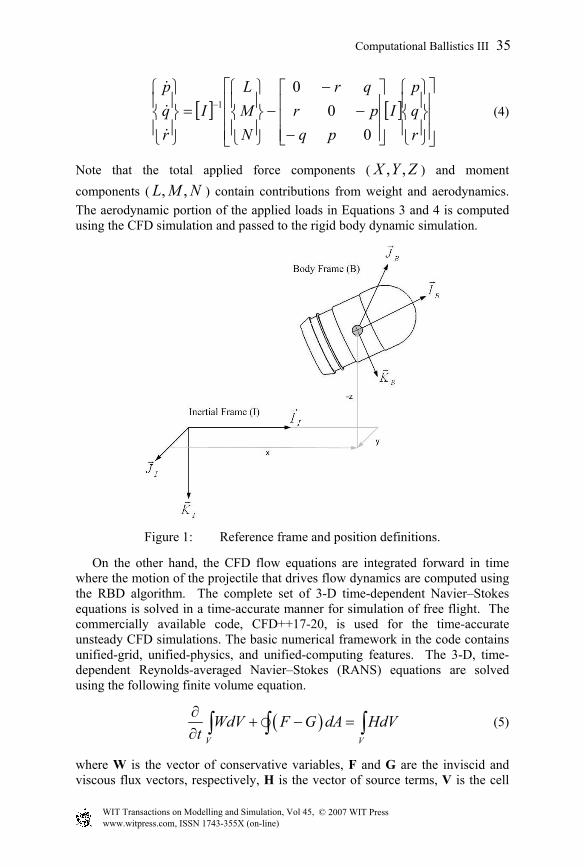
The projectile CFD/RBD algorithm employed here combines a rigid six degree of freedom projectile flight dynamic model with a three dimensional, time accurate CFD simulation. The RBD dynamic equations are integrated forward in time where aerodynamic forces and moments that drive motion of the projectile are computed using the CFD algorithm. The RBD projectile model allows for 3 translation degrees of freedom and 3 rotation degrees of freedom. As shown in Figure 1, the I frame is attached to the ground while the B frame is fixed to the projectile with the BI axis
pointing out the nose of the projectile and the BJ and BK unit vectors forming a right handed triad. The projectile state vector is comprised of the inertial position components of the projectile mass center ( , ,x y z ), the standard aerospace sequence Euler angles ( , ,φ θ ψ ), the body frame components of the projectile mass center velocity ( , ,u v w ), and the body frame components of the projectile angular velocity vector ( , ,p q r ). Both the translational and rotational dynamic equations are expressed in the projectile body reference frame. The standard rigid projectile, body frame equations of motion are given by Equations 1 through 4.
−−++−
=
wvu
cccsscssscccsssscsscscsccsscc
zyx
θφθφθ
ψφψθφψφψθφψθ
ψφψθφψφψθφψθ
(1)
−=
rqp
cccssctcts
θφθφ
φφ
θφθφ
ψθφ
//001
(2)
−−
−−
=
wvu
pqpr
qr
mZmYmX
wvu
00
0
///
(3)
© 2007 WIT PressWIT Transactions on Modelling and Simulation, Vol 45, www.witpress.com, ISSN 1743-355X (on-line)
34 Computational Ballistics III
[ ] [ ]
−−
−−
=
−
rqp
Ipq
prqr
NML
Irqp
00
01 (4)
Note that the total applied force components ( , ,X Y Z ) and moment components ( , ,L M N ) contain contributions from weight and aerodynamics. The aerodynamic portion of the applied loads in Equations 3 and 4 is computed using the CFD simulation and passed to the rigid body dynamic simulation.
Figure 1: Reference frame and position definitions.
On the other hand, the CFD flow equations are integrated forward in time where the motion of the projectile that drives flow dynamics are computed using the RBD algorithm. The complete set of 3-D time-dependent Navier–Stokes equations is solved in a time-accurate manner for simulation of free flight. The commercially available code, CFD++17-20, is used for the time-accurate unsteady CFD simulations. The basic numerical framework in the code contains unified-grid, unified-physics, and unified-computing features. The 3-D, time-dependent Reynolds-averaged Navier–Stokes (RANS) equations are solved using the following finite volume equation.
( )V V
WdV F G dA HdVt∂
+ − =∂ ∫ ∫ ∫ (5)
where W is the vector of conservative variables, F and G are the inviscid and viscous flux vectors, respectively, H is the vector of source terms, V is the cell
© 2007 WIT PressWIT Transactions on Modelling and Simulation, Vol 45, www.witpress.com, ISSN 1743-355X (on-line)
Computational Ballistics III 35
volume, and A is the surface area of the cell face. A second-order discretization is used for the flow variables and the turbulent viscosity equation. The turbulence closure is based on topology-parameter-free formulations. Two-equation higher order RANS turbulence models are used for the computation of turbulent flows. These models are ideally suited to unstructured book-keeping and massively parallel processing due to their independence from constraints related to the placement of boundaries and/or zonal interfaces. A dual time-stepping approach is used to integrate the flow equations to achieve the desired time-accuracy. The first is an “outer” or global (and physical) time step that corresponds to the time discretization of the physical time variation term. This time step can be chosen directly by the user and is typically set to a value to represent 1/100 of the period of oscillation expected or forced in the transient flow. It is also applied to every cell and is not spatially varying. An artificial or “inner” or “local” time variation term is added to the basic physical equations. This time step and corresponding “inner-iteration” strategy is chosen to help satisfy the physical transient equations to the desired degree. For the inner iterations, the time step is allowed to vary spatially. Also, relaxation with multigrid (algebraic) acceleration is employed to reduce the residues of the physical transient equations. It is found that an order of magnitude reduction in the residues is usually sufficient to produce a good transient iteration. The projectile in the coupled CFD/RBD simulation along with its grid moves and rotates as the projectile flies downrange. Grid velocity is assigned to each mesh point. For a spinning and yawing projectile, the grid speeds are assigned as if the grid is attached to the projectile and spinning and yawing with it. In order to properly initialize the CFD simulation, two modes of operation for the CFD code are utilized, namely, an uncoupled and a coupled mode. The uncoupled mode is used to initialize the CFD flow solution while the coupled mode represents the time accurate coupled CFD/RBD solution. In the uncoupled mode, the rigid body dynamics are specified. The uncoupled mode begins with a computation performed in “steady state mode” with the grid velocities prescribed to account for the proper initial position ( 0 0 0, ,x y z ), orientation ( 0 0 0, ,φ θ ψ ),
and translational velocity ( 0 0 0, ,u v w ) components of the complete set of initial conditions to be prescribed. After the quasi-steady state solution is converged, the initial spin rate ( 0p ) is included and a new quasi-steady state solution is obtained. A sufficient number of time steps are performed so that the angular orientation for the spin axis corresponds to the prescribed initial conditions. This steady state flow solution is the starting point for the coupled solution. For the coupled solution, the mesh is translated back to the desired initial position ( 0 0 0, ,x y z ) and the remaining angular velocity initial conditions ( 0 0,q r ) are then added. In the coupled mode, the aerodynamic forces and moments are passed to the RBD simulation which propagates the rigid state of the projectile forward in time.
© 2007 WIT PressWIT Transactions on Modelling and Simulation, Vol 45, www.witpress.com, ISSN 1743-355X (on-line)
36 Computational Ballistics III
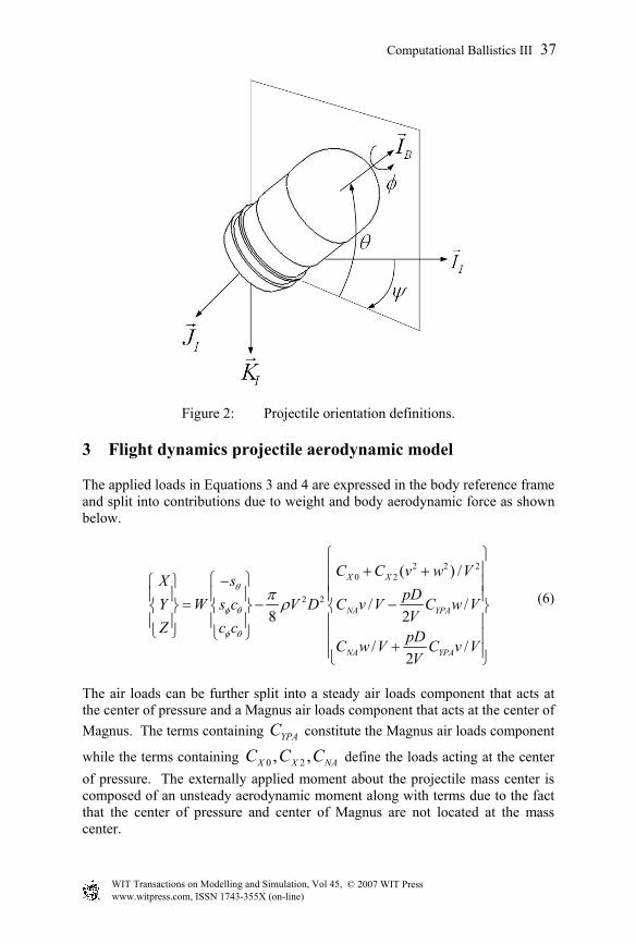
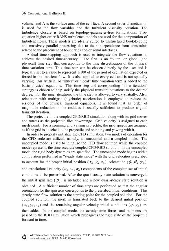
Figure 2: Projectile orientation definitions.
3 Flight dynamics projectile aerodynamic model
The applied loads in Equations 3 and 4 are expressed in the body reference frame and split into contributions due to weight and body aerodynamic force as shown below.
2 2 20 2
2 2
( ) /
/ /8 2
/ /2
X X
NA YPA
NA YPA
C C v w VX spDY W s c V D C v V C w VV
Z c c pDC w V C v VV
θ
φ θ
φ θ
π ρ
+ + −
= − − +
(6)
The air loads can be further split into a steady air loads component that acts at the center of pressure and a Magnus air loads component that acts at the center of Magnus. The terms containing YPAC constitute the Magnus air loads component
while the terms containing 0 2, ,X X NAC C C define the loads acting at the center of pressure. The externally applied moment about the projectile mass center is composed of an unsteady aerodynamic moment along with terms due to the fact that the center of pressure and center of Magnus are not located at the mass center.
© 2007 WIT PressWIT Transactions on Modelling and Simulation, Vol 45, www.witpress.com, ISSN 1743-355X (on-line)
Computational Ballistics III 37
2 3
2
8 2 2
2 2
LDD LP
MA MQ NPA
MA MQ NPA
pDC CVL
w qD pD vM V D C C CV V V V
N v rD pD wC C CV V V V
π ρ
+ = + + − + +
(7)
The terms involving MAC accounts for the center of pressure being located off
the mass center while the terms involving NPAC accounts for the center of Magnus being located off the mass center. In Equations 1 and 2, the aerodynamic coefficients and the distances from the aerodynamic force components to the projectile mass center are all a function of local Mach number. Typically in flight dynamic trajectory computer codes, this dependence on Mach number is handled through a table look-up scheme.
4 Aerodynamic coefficient estimation
The time accurate coupled CFD/RBD simulation provides a full flow solution including the aerodynamic portion of the total applied force and moment ( , , , , ,X Y Z L M N ) along with the full state of the rigid projectile ( , , , , , , , , , , ,x y z u v w p q rφ θ ψ ) at each time step in the solution. The rigid state of the projectile is used to obtain the weight portion of the applied force so that the aerodynamic force can be isolated. Using the information provided by the coupled CFD/RBD simulation, it is desired to compute all aerodynamic coefficients: 0 2, , ,X X NA YPAC C C C , , , , ,LDD LP MA MQ NPAC C C C C . For a fin-stabilized projectile, the Magnus force and moment are usually sufficiently small so that YPAC and NPAC are set to zero and removed from the fitting procedure to be described below. To estimate the aerodynamic coefficients near a particular Mach number, a set of n time accurate coupled CFD/RBD simulations are created over a relatively short time period. The initial conditions for the set of n time histories are generated to produce a rich database of aerodynamic loads and projectile states so that a unique solution can be obtained for the aerodynamic coefficients. The initial conditions for the rigid projectile states are Gaussian random numbers with a mean and standard deviation selected to cover normal operating conditions for the projectile. Since the aerodynamic coefficients to be estimated depend on local Mach number, the set of n time histories is repeated at m different Mach numbers of interest. Thus a total of *n m short time accurate coupled CFD/RBD trajectories are generated to support computation of a complete set of aerodynamic coefficients for flight dynamic simulation.
© 2007 WIT PressWIT Transactions on Modelling and Simulation, Vol 45, www.witpress.com, ISSN 1743-355X (on-line)
38 Computational Ballistics III
Since initial conditions for a given set of n time histories are randomly generated and because Mach number changes during a simulation, Mach number varies slightly even for a set of time histories intended to be generated at a particular Mach number. Hence, at a particular Mach number, all aerodynamic coefficients are assumed to vary linearly with Mach number. Parameters at intermediate values of Mach number were linearly interpolated as shown,
( )( ) M MC M C C CM M
−− + −
+ −
−= + −
− (8)
where C− and C+ are the aerodynamic coefficient values at Mach numbers
slightly less than ( M − ) and slightly greatly than ( M + ) the target Mach number. This general form for the aerodynamic coefficients is then substituted into the aerodynamic force and moment equations. Note that all aerodynamic coefficients that are to be estimated appear in the force and moment equations in a linear fashion suggesting a linear least squares approach to estimate the aerodynamic coefficients at each Mach number. Define the vectors XP , YZP , LP , and MNP as vectors containing all the unknown aerodynamic coefficients that are to be estimated at a given target Mach number. 0 0 2 2X X X X XP C C C C− + − + = (9)
YZ NA NA YPA YPAP C C C C− + − + = (10)
L LP LP LDD LDDP C C C C− + − + = (11)
MN MA MA MQ MQ NPA NPAP C C C C C C− + − + − + = (12)
Denote the total number of unknowns as j . For a fin stabilized projectile,
14j = while for a spin stabilized projectile 18j = . Assuming each time history contains k time simulation output points, then *k n linear equations in j unknowns are generated at each target Mach number.
X X XA P B= (13) YZ YZ YZA P B= (14)
© 2007 WIT PressWIT Transactions on Modelling and Simulation, Vol 45, www.witpress.com, ISSN 1743-355X (on-line)
Computational Ballistics III 39
L L LA P B= (15)
MN MN MNA P B= (16) Provided the matrices XA , YZA , LA , and MNA are maximal rank, a unique
solution for XP , YZP , LP , and MNP exists. Thus, properties of the matrices above, such as the rank or singular values, can be used as an indicator of the suitability of the CFD/RBD simulation data in estimating the aerodynamic coefficients at the target Mach number.
5 Results
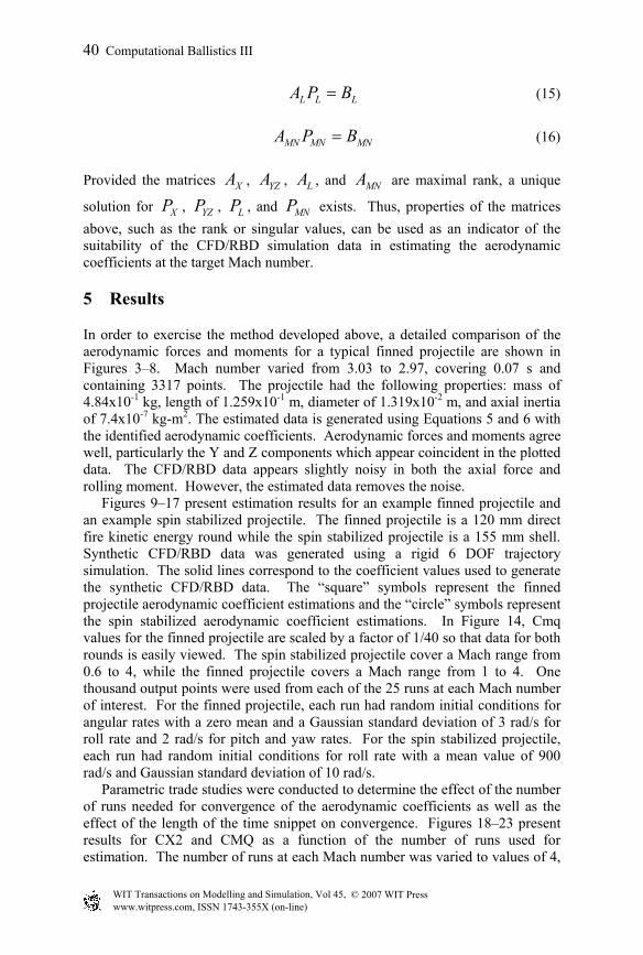
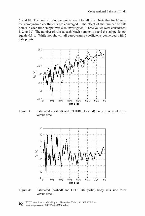
In order to exercise the method developed above, a detailed comparison of the aerodynamic forces and moments for a typical finned projectile are shown in Figures 3–8. Mach number varied from 3.03 to 2.97, covering 0.07 s and containing 3317 points. The projectile had the following properties: mass of 4.84x10⁻¹ kg, length of 1.259x10⁻¹ m, diameter of 1.319x10⁻² m, and axial inertia of 7.4x10⁻⁷ kg-m2. The estimated data is generated using Equations 5 and 6 with the identified aerodynamic coefficients. Aerodynamic forces and moments agree well, particularly the Y and Z components which appear coincident in the plotted data. The CFD/RBD data appears slightly noisy in both the axial force and rolling moment. However, the estimated data removes the noise. Figures 9–17 present estimation results for an example finned projectile and an example spin stabilized projectile. The finned projectile is a 120 mm direct fire kinetic energy round while the spin stabilized projectile is a 155 mm shell. Synthetic CFD/RBD data was generated using a rigid 6 DOF trajectory simulation. The solid lines correspond to the coefficient values used to generate the synthetic CFD/RBD data. The “square” symbols represent the finned projectile aerodynamic coefficient estimations and the “circle” symbols represent the spin stabilized aerodynamic coefficient estimations. In Figure 14, Cmq values for the finned projectile are scaled by a factor of 1/40 so that data for both rounds is easily viewed. The spin stabilized projectile cover a Mach range from 0.6 to 4, while the finned projectile covers a Mach range from 1 to 4. One thousand output points were used from each of the 25 runs at each Mach number of interest. For the finned projectile, each run had random initial conditions for angular rates with a zero mean and a Gaussian standard deviation of 3 rad/s for roll rate and 2 rad/s for pitch and yaw rates. For the spin stabilized projectile, each run had random initial conditions for roll rate with a mean value of 900 rad/s and Gaussian standard deviation of 10 rad/s. Parametric trade studies were conducted to determine the effect of the number of runs needed for convergence of the aerodynamic coefficients as well as the effect of the length of the time snippet on convergence. Figures 18–23 present results for CX2 and CMQ as a function of the number of runs used for estimation. The number of runs at each Mach number was varied to values of 4,
© 2007 WIT PressWIT Transactions on Modelling and Simulation, Vol 45, www.witpress.com, ISSN 1743-355X (on-line)
40 Computational Ballistics III
6, and 10. The number of output points was 1 for all runs. Note that for 10 runs, the aerodynamic coefficients are converged. The effect of the number of data points in each time snippet was also investigated. Three values were considered: 1, 2, and 5. The number of runs at each Mach number is 6 and the snippet length equals 0.1 s. While not shown, all aerodynamic coefficients converged with 5 data points.
Figure 3: Estimated (dashed) and CFD/RBD (solid) body axis axial force versus time.
Figure 4: Estimated (dashed) and CFD/RBD (solid) body axis side force versus time.
© 2007 WIT PressWIT Transactions on Modelling and Simulation, Vol 45, www.witpress.com, ISSN 1743-355X (on-line)
Computational Ballistics III 41
Figure 5: Estimated (dashed) and CFD/RBD (solid) body axis vertical force versus time.
Figure 6: Estimated (dashed) and CFD/RBD (solid) body axis rolling moment versus time.
© 2007 WIT PressWIT Transactions on Modelling and Simulation, Vol 45, www.witpress.com, ISSN 1743-355X (on-line)
42 Computational Ballistics III
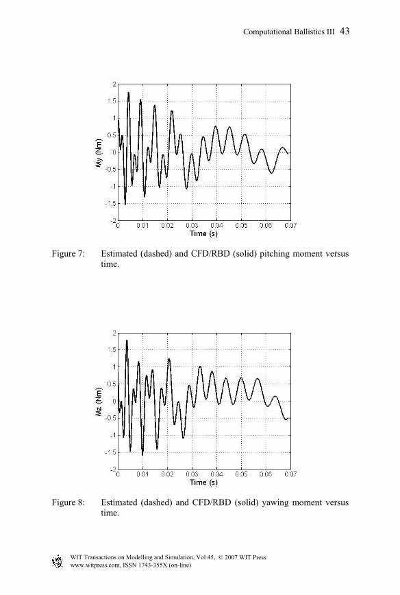
Figure 7: Estimated (dashed) and CFD/RBD (solid) pitching moment versus time.
Figure 8: Estimated (dashed) and CFD/RBD (solid) yawing moment versus time.
© 2007 WIT PressWIT Transactions on Modelling and Simulation, Vol 45, www.witpress.com, ISSN 1743-355X (on-line)
Computational Ballistics III 43
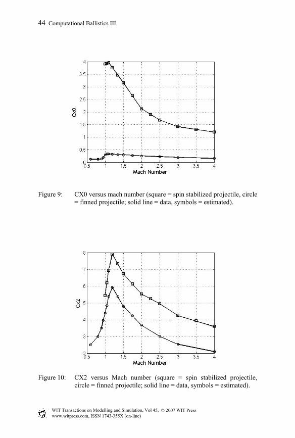
Figure 9: CX0 versus mach number (square = spin stabilized projectile, circle = finned projectile; solid line = data, symbols = estimated).
Figure 10: CX2 versus Mach number (square = spin stabilized projectile, circle = finned projectile; solid line = data, symbols = estimated).
© 2007 WIT PressWIT Transactions on Modelling and Simulation, Vol 45, www.witpress.com, ISSN 1743-355X (on-line)
44 Computational Ballistics III
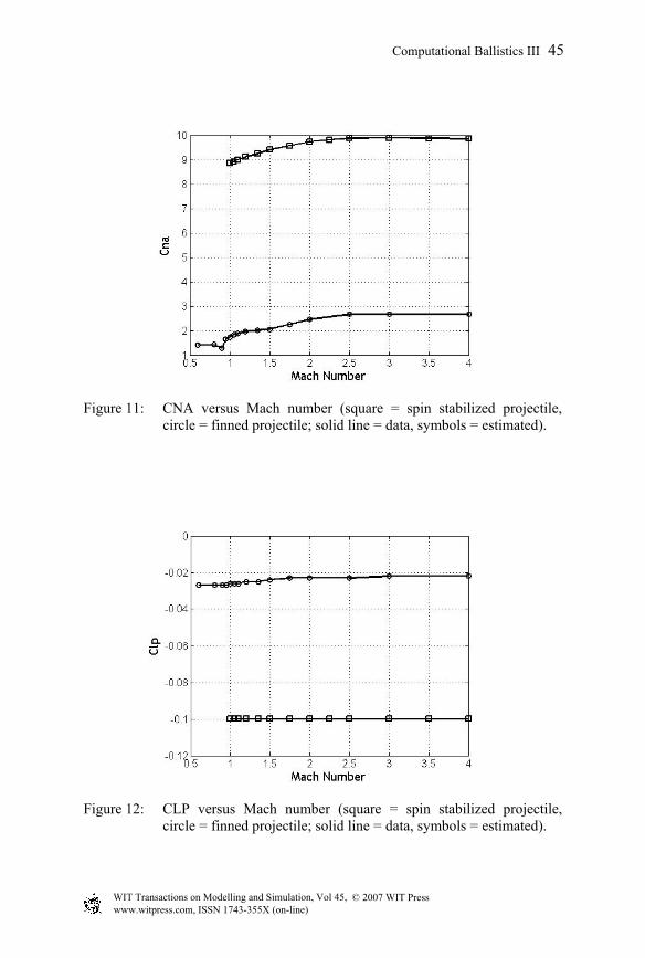
Figure 11: CNA versus Mach number (square = spin stabilized projectile, circle = finned projectile; solid line = data, symbols = estimated).
Figure 12: CLP versus Mach number (square = spin stabilized projectile, circle = finned projectile; solid line = data, symbols = estimated).
© 2007 WIT PressWIT Transactions on Modelling and Simulation, Vol 45, www.witpress.com, ISSN 1743-355X (on-line)
Computational Ballistics III 45
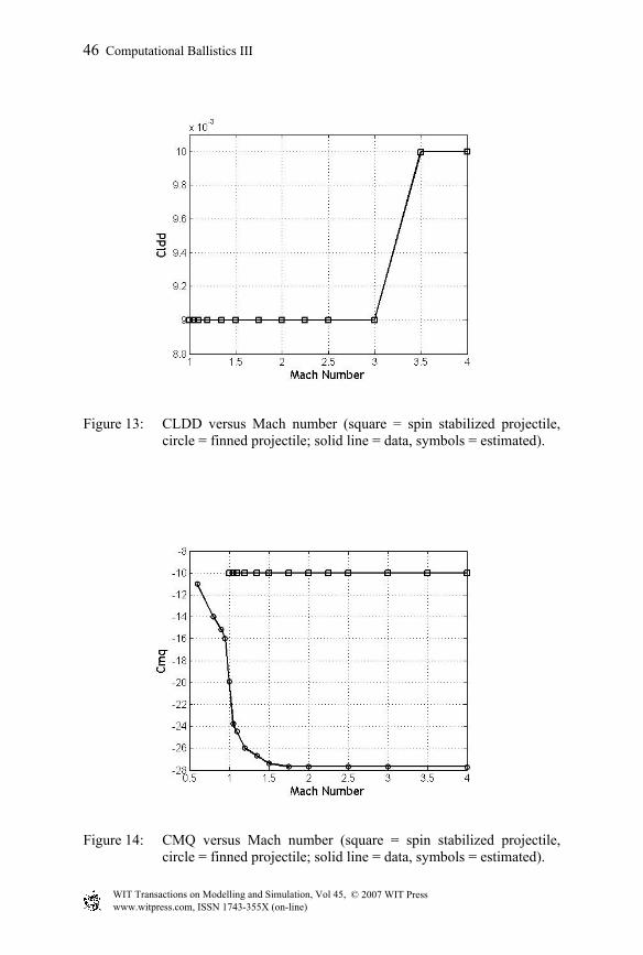
Figure 13: CLDD versus Mach number (square = spin stabilized projectile, circle = finned projectile; solid line = data, symbols = estimated).
Figure 14: CMQ versus Mach number (square = spin stabilized projectile, circle = finned projectile; solid line = data, symbols = estimated).
© 2007 WIT PressWIT Transactions on Modelling and Simulation, Vol 45, www.witpress.com, ISSN 1743-355X (on-line)
46 Computational Ballistics III
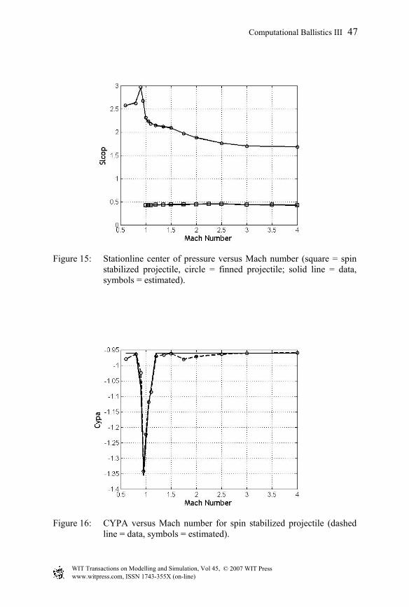
Figure 15: Stationline center of pressure versus Mach number (square = spin stabilized projectile, circle = finned projectile; solid line = data, symbols = estimated).
Figure 16: CYPA versus Mach number for spin stabilized projectile (dashed line = data, symbols = estimated).
© 2007 WIT PressWIT Transactions on Modelling and Simulation, Vol 45, www.witpress.com, ISSN 1743-355X (on-line)
Computational Ballistics III 47
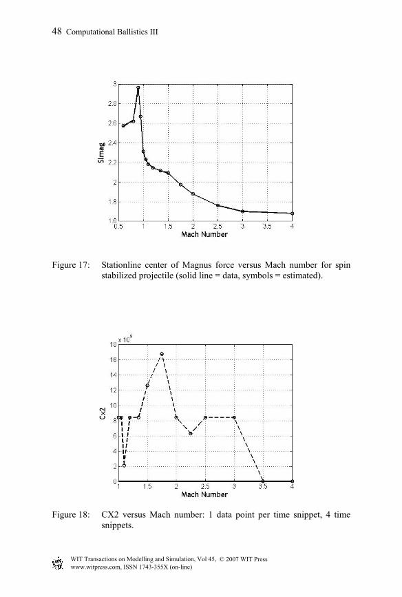
Figure 17: Stationline center of Magnus force versus Mach number for spin stabilized projectile (solid line = data, symbols = estimated).
Figure 18: CX2 versus Mach number: 1 data point per time snippet, 4 time snippets.
© 2007 WIT PressWIT Transactions on Modelling and Simulation, Vol 45, www.witpress.com, ISSN 1743-355X (on-line)
48 Computational Ballistics III
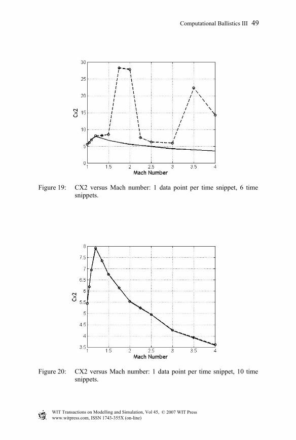
Figure 19: CX2 versus Mach number: 1 data point per time snippet, 6 time snippets.
Figure 20: CX2 versus Mach number: 1 data point per time snippet, 10 time snippets.
© 2007 WIT PressWIT Transactions on Modelling and Simulation, Vol 45, www.witpress.com, ISSN 1743-355X (on-line)
Computational Ballistics III 49
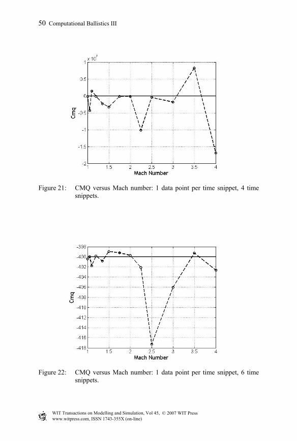
Figure 21: CMQ versus Mach number: 1 data point per time snippet, 4 time snippets.
Figure 22: CMQ versus Mach number: 1 data point per time snippet, 6 time snippets.
© 2007 WIT PressWIT Transactions on Modelling and Simulation, Vol 45, www.witpress.com, ISSN 1743-355X (on-line)
50 Computational Ballistics III
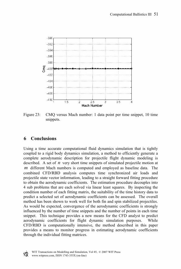
Figure 23: CMQ versus Mach number: 1 data point per time snippet, 10 time snippets.
Using a time accurate computational fluid dynamics simulation that is tightly coupled to a rigid body dynamics simulation, a method to efficiently generate a complete aerodynamic description for projectile flight dynamic modeling is described. A set of n very short time snippets of simulated projectile motion at m different Mach numbers is computed and employed as baseline data. The combined CFD/RBD analysis computes time synchronized air loads and projectile state vector information, leading to a straight forward fitting procedure to obtain the aerodynamic coefficients. The estimation procedure decouples into 4 sub problems that are each solved via linear least squares. By inspecting the condition number of each fitting matrix, the suitability of the time history data to predict a selected set of aerodynamic coefficients can be assessed. The overall method has been shown to work well for both fin and spin stabilized projectiles. As would be expected, convergence of the aerodynamic coefficients is strongly influenced by the number of time snippets and the number of points in each time snippet. This technique provides a new means for the CFD analyst to predict aerodynamic coefficients for flight dynamic simulation purposes. While CFD/RBD is computationally intensive, the method described in this paper provides a means to monitor progress in estimating aerodynamic coefficients through the individual fitting matrices.
6 Conclusions
© 2007 WIT PressWIT Transactions on Modelling and Simulation, Vol 45, www.witpress.com, ISSN 1743-355X (on-line)
Computational Ballistics III 51
Nomenclature
zyx ,, : Components of position vector of mass center in an inertial reference frame.
ψθφ ,, : Euler roll, pitch, and yaw angles of box. wvu ,, : Components of velocity vector of mass center in body reference frame. rqp ,, : Components of angular velocity vector in body reference frame.
zyx FFF ,, : Total applied force components in body reference frame.
zyx MMM ,, : Total applied moment components about mass center in body reference frame. V : Magnitude of relative aerodynamic velocity vector of mass center. ρ : Air density. D : Projectile diameter. α : Aerodynamic angle of attack. Cx0: Zero yaw drag aerodynamic coefficient. Cx2: Yaw drag aerodynamic coefficient. Cna: Normal force due to angle of attack aerodynamic coefficient. Cypa: Magnus force aerodynamic coefficient. Clp: Roll damping aerodynamic coefficient. Cldd: Fin cant aerodynamic coefficient. Cmq: Pitch damping moment aerodynamic coefficient. Dcop: Distance from the mass center to the center of pressure. Dmag: Distance from the mass center to the center of Magnus. CFD: Computational Fluid Dynamics.
References
[1] J. Sun, R. Cummings, “Evaluation of Missile Aerodynamic Characteristics Using Rapid Prediction Techniques,” Journal of Spacecraft and Rockets, Vol 21, No 6, pp 513-520, 1984.
[2] F. Moore, “The 2005 Version of the Aeroprediction Code (AP05),” AIAA 2004-4715, AIAA Atmospheric Flight Mechanics Conference, Providence, Rhode Island, 2004.
[3] T. Sooy, R. Schmidt, “Aerodynamic Predictions, Comparisons, and Validations Using Missile DATCOM and Aeroprediction 98,” AIAA-2004-1246, AIAA Aerospace Sciences Meeting and Exhibit, Reno, Nevada, 2004.
[4] J. Simon, W. Blake, “Missile DATCOM – High Angle of Attack Capabilities,” AIAA-1999-4258, AIAA Atmospheric Flight Mechanics Conference, Portland, Oregon, 1999.
[5] A. Neely, I. Auman, “Missile DATCOM Transonic Drag Improvements for Hemispherical Nose Shapes,” AIAA-2003-3668, AIAA Applied Aerodynamics Conference, 2003.
© 2007 WIT PressWIT Transactions on Modelling and Simulation, Vol 45, www.witpress.com, ISSN 1743-355X (on-line)
52 Computational Ballistics III
[6] W. Blake, “Missile DATCOM – 1997 Status and Future Plans,” AIAA-1997-2280,” AIAA Applied Aerodynamics Conference, Atlanta, Georgia, 1997.
[7] A. Dupuis, C. Berner, “Wind Tunnel Tests of a Long Range Artillery Shell Concept,” AIAA-2002-4416, AIAA Atmospheric Flight Mechanics Conference, Monterey, California, 2002.
[8] C. Berner, A Dupuis, “Wind Tunnel Tests of a Grid Fin Projectile Configuration,” AIAA-2001-0105, AIAA Aerospace Sciences Meeting, Reno, Nevada, 2001.
[9] J. Evans, “Prediction of Tubular Projectile Aerodynamics Using the ZUES Euler Code,” Journal of Spacecraft and Rockets, Vol 26, No 5, pp 314-321, 1989,
[10] W. Sturek, C. Nietubicz, J. Sahu, P. Weinacht, “Applications of Computational Fluid Dynamics to the Aerodynamics of Army Projectiles, Journal of Spacecraft and Rockets, Vol 31, No 2, pp 186-199, 1994.
[11] M. Nusca, S. Chakravarthy, U. Goldberg, “Computational Fluid Dynamics Capability for the Solid-Fuel Ramjet Projectile,” Journal of Propulsion and Power, Vol 6, No 3, 1990.
[12] S. Silton, “Navier-Stokes Computations for a Spinning Projectile from Subsonic to Supersonic Speeds,” Journal of Spacecraft and Rockets, Vol 42, No 2, pp 223-231, 2005.
[13] J. DeSpirito, M. Vaughn, D. Washington, “Numerical Investigation of Canard-Controlled Missile with Planar Grid Fins,” Journal of Spacecraft and Rockets, Vol 40, No 3, pp 363-370, 2003.
[14] M. Graham, P. Weinacht, J. Bennett, “Numerical Investigation of Supersonic Jet Interaction for Finned Bodies, Journal of Spacecraft and Rockets, Vol 37, No 5, pp 675-683, 2000.
[15] P. Weinacht, “Navier-Stokes Prediction of the Individual Components of the Pitch Damping Sum,” Journal of Spacecraft and Rockets, Vol 35, No 5, pp 598-605, 1998.
[16] B. Guidos, P. Weinacht, D. Dolling, “Navier-Stokes Computations for Pointed, Spherical, and Flat Tipped Shells at Mach 3,“ Journal of Spacecraft and Rockets, Vol 29, No 3, pp 305-311, 1992.
[17] P. Weinacht, W. Sturek, “Computation of the Roll Characteristics of a Finned Projectile,” Journal of Spacecraft and Rockets, Vol 33, No 6, pp 769-775, 1996.
[18] S. Park, J. Kwon, “Navier-Stokes Computations of Stability Derivatives for symmetric Projectiles, AIAA-2004-0014, AIAA Aerospace Sciences Meeting, Reno, Nevada, 2004.
[19] N. Qin, K. Ludlow, S. Shaw, J. Edwards, A. Dupuis, “Calculation of Pitch Damping for a Flared Projectile,” Journal of Spacecraft and Rockets, Vol 34, No 4, pp 566-568, 1997.
[20] P. Weinacht, “Coupled CFD/GN&C Modeling for a Smart Material Canard Actuator,” AIAA-2004-4712, AIAA Atmospheric Flight Mechanics Conference, Providence, Rhode Island, 2004.
© 2007 WIT PressWIT Transactions on Modelling and Simulation, Vol 45, www.witpress.com, ISSN 1743-355X (on-line)
Computational Ballistics III 53
[21] S. Park, Y. Kim, J. Kwon, “Prediction of Dynamic Damping Coefficients Using Unsteady Dual Time Stepping Method,“ AIAA-2002-0715, AIAA Aerospace Sciences Meeting, Reno, Nevada, 2002.
[22] J. DeSpirito, K. Heavey, ”CFD Computation of Magnus Moment and Roll-Damping Moment of a Spinning Projectile,” AIAA-2004-4713, AIAA Atmospheric Flight Mechanics Conference, Providence, Rhode Island, 2004.
[23] K. Garon, G. Abate, W. Hathaway, “Free-Flight Testing of a Generic Missile with MEMs Protuberances,” AIAA -2003-1242, AIAA Aerospace Sciences Meeting, Reno, Nevada, 2003.
[24] B. Kruggel, “High Angle of Attack Free Flight Missile Testing,” AIAA-1999-0435, AIAA Aerospace Sciences Meeting, Reno, Nevada, 1999.
[25] J. Danberg, A. Sigal, I. Clemins, “Aerodynamic Characteristics of a Family of Cone-Cylinder-Flare Projectiles, Journal of Spacecraft and Rockets, Vol 27, No 4, 1990.
[26] A. Dupuis, “Free-Flight Aerodynamic Characteristics of a Practice Bomb at Subsonic and Transonic Velocities,” AIAA-2002-4414, AIAA Atmospheric Flight Mechanics Conference, Monterey, California, 2002.
[27] G. Abate, R. Duckerschein, W. Hathaway, “Subsonic/transonic Free-Flight Tests of a Generic Missile with Grid Fins, AIAA-2000-0937, AIAA Aerospace Sciences Meeting, Reno, Nevada, 2000.
[28] G. Chapman, D. Kirk, “A Method for Extracting Aerodynamic Coefficients from Free-Flight Data,” AIAA Journal, Vol 8, No 4, pp 753-758, 1970.
[29] G. Abate, A. Klomfass, “Affect upon Aeroballistic Parameter Identification from Flight Data Errors,” AIAA Aerospace Sciences Meeting, Reno, Nevada, 2005.
[30] G. Abate, A. Klomfass, “A New Method for Obtaining Aeroballistic Parameters from Flight Data,” Aeroballistic Range Association Meeting, Freiburg, Germany, 2004.
[31] P. Weinacht, W. Sturek, L. Schiff, “Projectile Performance, Stability, and Free-Flight Motion Prediction Using Computational Fluid Dynamics,“ Journal of Spacecraft and Rockets, Vol 41, No 2, pp 257-263, 2004.
[32] J. Sahu, “Time-Accurate Numerical Prediction of Free-Flight Aerodynamics of a Finned Projectile,” AIAA-2005-5817, AIAA Atmospheric Flight Mechanics Conference, San Francisco, California, 2005.
[33] G. Abate, A. Klomfass, “Affect upon Aeroballistic Parameter Identification from Flight Data Errors,” AIAA-2005-0439, AIAA Aerospace Sciences Meeting, Reno, Nevada, 2005.
© 2007 WIT PressWIT Transactions on Modelling and Simulation, Vol 45, www.witpress.com, ISSN 1743-355X (on-line)
54 Computational Ballistics III