Generalized smoothing splines and the optimal ...big · Generalized smoothing splines and the...
31
To appear in IEEE TRANSACTIONS ON SIGNAL PROCESSING 1 Generalized smoothing splines and the optimal discretization of the Wiener filter Michael Unser and Thierry Blu The authors are with the Biomedical Imaging Group, STI-IOA, Swiss Federal Institute of Technology, Lausanne (EPFL), CH-1015 Lausanne, Switzerland (e-mail: [email protected], phone: +41 21 693 51 43, fax: +41 21 693 37 01) July 1, 2004 DRAFT
Transcript of Generalized smoothing splines and the optimal ...big · Generalized smoothing splines and the...

To appear inIEEE TRANSACTIONS ON SIGNAL PROCESSING 1
Generalized smoothing splines and the optimal
discretization of the Wiener filter
Michael Unser and Thierry Blu
The authors are with the Biomedical Imaging Group, STI-IOA, Swiss Federal Institute of Technology, Lausanne (EPFL),
CH-1015 Lausanne, Switzerland (e-mail: [email protected], phone: +41 21 693 51 43, fax: +41 21 693 37 01)
July 1, 2004 DRAFT
To appear inIEEE TRANSACTIONS ON SIGNAL PROCESSING 2
Abstract
We introduce an extended class of cardinalL∗L-splines whereL is a pseudo-differential operator satisfying some
admissibility conditions. We show that theL∗L-spline signal interpolation problem is well posed and that its solution
is the unique minimizer of the spline energy functional,‖Ls‖2L2 , subject to the interpolation constraint. Next, we
consider the corresponding regularized least squares estimation problem, which is more appropriate for dealing with
noisy data. The criterion to be minimized is the sum of a quadratic data term, which forces the solution to be close
to the input samples, and a “smoothness” term that privileges solutions with small spline energies. Here too, we
find that the optimal solution, among all possible functions, is a cardinalL∗L-spline. We show that this smoothing
spline estimator has a stable representation in a B-spline-like basis and that its coefficients can be computed by
digital filtering of the input signal. We describe an efficient recursive filtering algorithm that is applicable whenever
the transfer function ofL is rational (which corresponds to the case of exponential splines).
We justify these algorithms statistically by establishing an equivalence betweenL∗L smoothing splines and
the MMSE (minimum mean square error) estimation of a stationary signal corrupted by white Gaussian noise. In
this model-based formulation, the optimum operatorL is the whitening filter of the process, and the regularization
parameter is proportional to the noise variance. Thus, the proposed formalism yields the optimal discretization of the
classical Wiener filter, together with a fast recursive algorithm. It extends the standard Wiener solution by providing
the optimal interpolation space. We also present a Bayesian interpretation of the algorithm.
Index Terms
Smoothing splines, splines (polynomial and exponential), Wiener filter, Variational principle, non-
parametric estimation, recursive filtering, stationary processes
I. I NTRODUCTION
In a series of companion papers, we have introduced a general continuous/discrete approach to signal
processing that uses an exponential B-spline representation of signals [1], [2]. A key feature of this
framework is that it allows one to implement continuous-time signal processing operations exactly, and
quite efficiently, by simple discrete processing of the B-spline coefficients of the signal. Its main advantage
over the traditional bandlimited approach is that the underlying basis functions are compactly supported.
The E-spline framework offers the choice of a large variety of basis functions, which are specified in
terms of their poles and zeros, and which constitute a considerable extension of the standard, piecewise
polynomial ones. While the availability of such a rich collection of signal models provides many new
design opportunities, it also raises the issue of the selection of the most appropriate one for a given
application. One possible criterion is to favor simplicity and to choose the input signal representation
(e.g. piecewise constant or linear) that minimizes algorithmic complexity. Another option, which is the
one developed in this paper, is to optimize the choice of the signal space based on the characteristics
July 1, 2004 DRAFT

To appear inIEEE TRANSACTIONS ON SIGNAL PROCESSING 3
(e.g., general smoothness properties or prior statistical distribution) of the class of continuous-time signals
from which the measurements (discrete samples) are derived. This can be accomplished in essentially
two ways: (a) within a deterministic framework by searching for a solution that minimizes some suitable
smoothness energy functional, and (b) within a stochastic framework by deriving a Bayesian or a minimum
mean square error (MMSE) estimator of the signal. Similar to what has been noted in the related area
of image restoration [3]–[5], we will see that these various points of views (which may be referred to as
Lagrange/Tikhonov, Bayesian and Wiener) are mathematically equivalent, and that they lead to generalized
spline solutions that can be determined by digital filtering techniques. We will also take advantage of
the proposed formalism to specify a rather general class of spline estimators that can handle noisy input
data, similar to the classical smoothing splines proposed by Schoenberg and Reinsh [6], [7].
The model-based approach to splines that we are suggesting has its roots in approximation theory:
There is an extensive literature that deals with the variational aspects of splines and even a whole sub-
branch of spline theory that uses the energy minimization property as starting point for the definition
of a generalized notion of spline [8]–[10]. This kind of formulation is also the one that carries over
best to multiple dimensions; for instance, it has led to the methods of thin-plate splines and radial basis
functions [11]–[13], which have become quite popular for the interpolation of scattered data in multiple
dimensions.
The equivalence between variational splines and statistical estimation techniques—in particular, Bayesian
ones—has been recognized early on [14], [15]. Smoothing splines and their multidimensional extensions
have been studied in depth by Wahba who used a powerful Reproducing-Kernel-Hilbert-Space formulation
[16]; these efforts led to a variety of non-parametric linear estimation techniques which are now widely
used in statistics [17]–[19]. Somewhat lesser known is the work of Weinert who uncovered the connection
between spline interpolation and MMSE estimation and who used this formal link to derive Kalman-type
recursive smoothing algorithms [20], [21]. Also relevant to the issue is the theoretical connection that
exists between spline estimation techniques and the kriging methods that were developed in geostatistics
for the interpolation of scattered data [22]–[24].
Unfortunately, the adaptation of these mathematical results to the cardinal framework is not straight-
forward. The major difficulty is that the above mentioned formulations all consider a finite number
of samples—these cannot be simply transposed to infinite dimensions without resolving some delicate
convergence and stability issues. In addition, the generality of some of the methods (they consider non-
uniform samples as well as space-varying differential models) is such that it does not facilitate the
identification of fast computational schemes. This is a typical situation where it is more efficient to
July 1, 2004 DRAFT

To appear inIEEE TRANSACTIONS ON SIGNAL PROCESSING 4
formulate the constrained version of the problem and to derive the solution we are seeking. This justifies
our present effort which is to revisit the variational aspects of splines within the cardinal framework. As
in our previous work, we apply a signal processing formulation and take advantage of the shift-invariant
structure of the problem, with the following benefits:
• Simplification of the theory: even though there are a few technicalities associated with the infinite
dimensionality of the data sequences, we can simplify the mathematics by applying Fourier tech-
niques. In particular, there is no more need for a special treatment of the homogeneous component
of the solution (in our view, the most delicate aspect of the classical formulation) because there are
no boundary conditions.
• Generality: The Fourier domain formulation allows us to consider a larger class of spline-defining
(pseudo-differential) operators than what is done usually—with the restriction that they need to be
shift-invariant.
• Self-contained formulation: The present derivations and algorithms can all be explained in standard
signal processing terms, making them accessible and more appealing to this community.
• New computational solutions and link with standard signal processing methods: as in our previous
work, we can solve the spline fitting problems using digital filters. The formulation also yields an
optimal discretization of the classical Wiener filter.
The paper is organized as follows. In Section II, we start with a brief exposition of the key mathematical
notions that are required for this paper. In Section III, we enlarge our previous family of cardinal E-
splines by introducing the notion ofspline-admissibleconvolution operator. We then consider the class
of positive-definite operatorsL∗L that yield generalized cardinal splines with interesting mathematical
properties. In Section IV, we show that theseL∗L-splines can also be specified via the minimization of a
pseudo-differential energy functional. We use this functional to define a smoothing spline estimator for
noisy signals. Taking advantage of the existence of a B-spline-like representation of these splines, we
derive efficient smoothing spline algorithms, extending our earlier results for polynomial splines [25]. In
Section V, we propose a statistical interpretation of the proposed spline fitting techniques. In particular,
we show that the smoothing spline algorithm solves the problem of the MMSE estimation of a stationary
signal corrupted by additive white noise. This result is important because it allows us to optimally tune
the parameters of the spline algorithm based on some a priori knowledge of second order statistics of the
signal and noise. It also yields a fast recursive implementation of the classical Wiener filter (cf. Eq. (18)
and Appendix II), as an interesting by-product. Finally, we also show how to recast the spline estimation
July 1, 2004 DRAFT
To appear inIEEE TRANSACTIONS ON SIGNAL PROCESSING 5
problem into a Bayesian framework, which is more in line with the interpretation of Kimeldorf and
Wahba [14].
II. PRELIMINARIES
We start with a presentation of the notations and mathematical tools that are used throughout the paper.
A. Continuous-time operators and function spaces
In our formulation, we consider an extended family of linear shift-invariant operatorsL which are
characterized by a convolution kernelL(t); i.e., Lf = L(t) ∗ f(t) where the argumentf = f(t) is a
continuous-time function witht ∈ R . We assume thatL(t) is a tempered distribution (i.e.,L ∈ S′) and
that its Fourier transform,F{L}(ω) = L(ω), is a true functionof ω. The adjoint operator is denoted by
L∗ and its impulse response isLT (t) := L(−t).
We classify the operatorsL according to an equivalent differentiation orderr.
Definition 1: The convolution operatorL is of orderr if and only if, for all positive realρ < r− 1/2,
we have that ∑n∈Z
|ω + 2nπ|2ρ
1 + |L(ω + 2nπ)|2≤ Cρ < ∞. (1)
A prototypical example of anrth order operator is therth fractional derivativeDr, whose frequency
response is(jω)r. An alternative notation isDrf = f (r).
To each operatorL, we associate a corresponding generalized Sobolev space
WL2 =
{f(t), t ∈ R :
∫ +∞
−∞|f(ω)|2
(1 + |L(ω)|2
)dω < +∞
}.
where f(ω) = F{f} =∫ +∞−∞ f(t)e−jωtdt is the Fourier transform off(t). For the particular choice
L = Dr, we recover the usual Sobolev spaces of orderr; i.e., WDr
2 = W r2 .
Our first result clarifies the link between the order of the operatorL and the classical notion of Sobolev
smoothness (for a proof, see Appendix I).
Theorem 1:Let L be a linear shift-invariant operator of orderr > 1/2 then, for all0 ≤ ρ < r − 1/2,
we have the properties:
i. WL2 ⊂ W ρ
2 ;
ii. if f ∈ WL2 , then the Poisson summation formula holds∑
n∈ZF{f (ρ)}(ω + 2nπ) =
∑n∈Z
f (ρ)(n)e−jnω almost everywhere;
iii. if f ∈ WL2 , then the integer samplesf (ρ)(n) are square summable:{f (ρ)(n)}n∈Z ∈ `2.
July 1, 2004 DRAFT

To appear inIEEE TRANSACTIONS ON SIGNAL PROCESSING 6
In particular, whenL is of smoothness orderr > 1/2, then the samplesf(n) of f ∈ WL2 are in `2.
B. Digital filters and sequence spaces
Discrete signals are indexed by the discrete variablek ∈ Z using square brackets to distinguish them
from their continuous-time counterparts. Such signals will be distinguished based on their appartenance
to the classical sequence spaces:`p ={a[k] : ‖a‖`p
< +∞}
with ‖a‖`p:=(∑
k∈Z |a[k]|p)1/p
for 1 ≤
p < ∞, and‖a‖`∞ := supk∈Z |a[k]|.
The digital filtering of a sequencea[k] yields the signal(h ∗ a)[k] =∑
l∈Z a[l]h[k − l] whereh is
the impulse response response of the filter; when the discrete context is obvious, we will sometimes
drop the time indices and simply writeh ∗ a. The digital filter can also be represented by its equivalent
continuous-time impulse responseh(t) =∑
k∈Z h[k]δ(t− k).
Here, we will only consider “stable” filters whose impulse responses are in`1. The frequency response
of such a filter, which is obtained by evaluating thez-transform ofh, H(z) =∑
k∈Z h[k]z−k, for z = ejω,
is guaranteed to be bounded and continuous [26].
An important related mathematical result is Young’s inequality,
‖h ∗ a‖`p≤ ‖h‖`1 · ‖a‖`p
, for 1 ≤ p ≤ +∞, (2)
which implies that the application of such a filter to an`p-sequence produces an output signal that is in
`p as well. For instance, by takingp = ∞, we can deduce that the digital filtering of a bounded input
(BI) signal produces a bounded output (BO) signal. In fact, there is a well known equivalence between
h ∈ `1 and BIBO-stability, where the latter property is crucial for signal processing applications [27],
[28]. Another direct consequence of Young’s inequality forp = 1 is that the cascade of two BIBO-stable
filters, h1 ∈ `1 andh2 ∈ `1, yields a filterh1 ∗h2 ∈ `1 that is BIBO-stable as well. Also note thath ∈ `1
implies thath has finite energy (i.e.,h ∈ `2), because of the inclusion property of the discrete`p spaces:
`p ⊂ `p′ , for 1 ≤ p ≤ p′ ≤ +∞.
The convolution inverse ofh will be denoted by(h)−1. A sufficient condition for the existence of this
inverse is provided by Wiener’s Lemma [29], which states that(h)−1 ∈ `1 if h ∈ `1 andH(ejω) 6= 0 for
∀ω ∈ [0, 2π]. Hence, the inverse filter is stable provided that the frequency response ofh is non-vanishing.
The adjoint operator ofh (real-valued) is the time-reversed filter whose impulse response is :hT [k] =
h[−k]. Indeed, we have the2-inner product relation
∀a, c ∈ `2, 〈a, h ∗ c〉`2 = 〈hT ∗ a, c〉`2 ,
July 1, 2004 DRAFT

To appear inIEEE TRANSACTIONS ON SIGNAL PROCESSING 7
which is established by simple change of summation variable.
C. Riesz bases
Cardinal splines provide a one-to-one mapping between discrete sequences and continuous-time func-
tions. A convenient mathematical way of describing this mapping is through the specification of a Riesz
basis for a given spline family. In the present context, the Riesz bases have a convenient integer-shift-
invariant structure:{ϕ(t − k)}k∈Z where the generatorϕ(t) is a generalized B-spline; typically, the
shortest possible (or most localized) spline within the given family. A standard result in sampling theory
is that the integer shifts of a functionϕ(t) ∈ L1 ∩ L2 form a Riesz basis1 if and only if there exist two
positive constantsAϕ andBϕ such that 0 < A2ϕ := infω∈[0,2π]
∑k∈Z |ϕ(ω + 2kπ)|2
B2ϕ := supω∈[0,2π]
∑k∈Z |ϕ(ω + 2kπ)|2 < +∞
(3)
whereϕ(ω) denotes the Fourier transform ofϕ(t). The corresponding function space, which is a subspace
of L2, is
V (ϕ) = {s(t) =∑k∈Z
c[k]ϕ(t− k) : c ∈ `2}. (4)
The Riesz basis conditions implies that we have an equivalence between theL2-norm of a signals(t) ∈
V (ϕ) and the`2-norm of its coefficientsc[k]:
Aϕ · ‖c‖`2 ≤
∥∥∥∥∥∑k∈Z
c[k]ϕ(t− k)
∥∥∥∥∥L2
≤ Bϕ · ‖c‖`2 ,
with equality if and only if the basis is orthonormal, that is, whenAϕ = Bϕ = 1.
In some instances—for example, when one is processing samples of a stationary process as in Section
V—one is interested in enlarging the space of admissible spliness(t) by allowing for B-spline coefficients
c[k] ∈ `∞. This is possible provided that the Riesz basis isLp-stable, that is, when there exist two positive
constants0 < Aϕ,p andBϕ,p < +∞ such that:
Aϕ,p · ‖c‖`p≤ ‖
∑k∈Z
c[k]ϕ(t− k)‖Lp≤ Bϕ,p · ‖c‖`p
,
for any 1 ≤ p ≤ ∞. It can be shown (cf. [30]) that a sufficient condition for an integer-shift-invariant
Riesz basis{ϕ(t− k)}k∈Z to beLp-stable (for all1 ≤ p ≤ +∞) is
Bϕ,p ≤ ‖ϕ‖L1,∞ := supt∈[0,1]
∑k∈Z
|ϕ(t + k)| < +∞, (5)
1The conditionϕ(t) ∈ L1 is not absolutely necessary, but it simplifies the formulation by ensuring that the sum in (3) is
continuous inω whenBϕ exists.
July 1, 2004 DRAFT

To appear inIEEE TRANSACTIONS ON SIGNAL PROCESSING 8
which adds a stronger constraint to (3). In particular, ourLp-stability condition,‖ϕ‖L1,∞ < +∞, implies
that ϕ(t) must be bounded and included inLp for all p ∈ [1,+∞]. Conversely, we note that (5) is
satisfied wheneverϕ(t) is bounded and decays faster thanO(1/|t|1+ε) with ε > 0. This is obviously the
case for the exponential B-splines described in [2], which are all compactly supported.
We now establish a Young-type convolution inequality for theLp-stability condition, which will be
required later on.
Proposition 1: Let ϕ1(t) andϕ2(t) be twoLp-stable functions. Then,
‖ϕ1 ∗ ϕ2‖L1,∞ ≤ ‖ϕ1‖L1,∞ · ‖ϕ2‖L1,∞ < +∞
Proof: We consider the following 1-periodic function int, which we bound from above:∑k∈Z
|(ϕ1 ∗ ϕ2)(t + k)| ≤∑k∈Z
∫ +∞
−∞|ϕ1(τ)| |ϕ2(t + k − τ)|dτ
=∑k∈Z
∑l∈Z
∫ 1
0|ϕ1(τ + l)| |ϕ2(t + k − τ − l)|dτ
=∫ 1
0
∑l∈Z
|ϕ1(τ + l)|∑k′∈Z
|ϕ2(t + k′ − τ)|dτ (Fubini′s Theorem)
≤ supτ∈[0,1]
∑l∈Z
|ϕ1(τ + l)| ·∫ 1
0
∑k′∈Z
|ϕ2(t + k′ − τ)|dτ
≤ supτ∈[0,1]
∑l∈Z
|ϕ1(τ + l)| · supt′∈[0,1]
∑k′∈Z
|ϕ2(t′ + k′)|,
where we have used the fact that the functions∑
l∈Z |ϕ1(τ +l)| and∑
k′∈Z |ϕ2(t+k′−τ)| are 1-periodic
in τ andt′ = t−τ , respectively, and where we have bounded them by their maximum within this period.
Since this inequality is true for allt, it also holds for the value oft at which the left hand side function
reaches its maximum, which yields the desired result.
III. L∗L-SPLINES AND CARDINAL INTERPOLATION
A. Spline-admissible operators
In our previous series of papers, we have investigated the cardinal exponential splines and have shown
how these can be specified via a differential operatorL whose transfer function can be expressed as a
polynomial in ω or, more generally, the ratio of two such polynomials. Here, we extend our class of
linear, shift-invariant operatorsL further to encompass an even wider family of splines. The operators that
we will be considering are referred to as “spline-admissible”; they must satisfy the following properties.
Definition 2: L is a spline-admissibleoperator of orderr if and only if
July 1, 2004 DRAFT
To appear inIEEE TRANSACTIONS ON SIGNAL PROCESSING 9
1) L is a linear shift-invariant operator of smoothness orderr > 1/2;
2) L has a well-defined inverseL−1 whose impulse responseρ(t) is a function of slow growth (i.e.,
ρ(t) ∈ S′). Thus,L admitsρ(t) as Green function:L{ρ} = δ(t).
3) There exists a corresponding spline-generating functionβ(t) = ∆L{ρ(t)} :=∑
k∈Z d[k]ρ(t − k)
(generalized B-spline) that satisfies the Riesz basis condition (3).
4) The localization operator∆L in 4) is a stable digital filter in the sense thatd ∈ `1.
5) The spline generatorβ(t) satisfies theLp-stability condition (5).
Properties 1) to 3) are quite explicit and easy to check. Properties 4) and 5) are less direct statements;
the most delicate issue is to establish that there is indeed a functionβ(t) in L2∩span{L−1{δ(t− k)}
}k∈Z
that satisfies the Riesz basis condition. This typically needs to be done on a case-by-case basis for a
given family of operators.
We will now elaborate some more on the crucial role played by the localization filter and justify the
use of this terminology. The Fourier transform ofβ(t) is given by
β(ω) =∆L(ejω)
L(ω)
so that a necessary requirement for it to be inL2 is that the localization filter∆L(ejω) =∑
k∈Z d[k]e−jωk
be such that is compensates for the potential singularities of the inverse filter1/L(ω). In particular, this
means that∆L(ejω) must locally have the same behavior asL(ω), especially around the frequencies where
L(ω) is vanishing. An important practical requirement is thatβ(ω) should have the largest possible degree
of continuity (ideally,β(ω) ∈ C∞) to guarantee thatβ(t) has very fast decay (ideally, compact support).
It also makes good sense to select a digital filter∆L(ejω) such thatβ(ω) is close to one over a reasonable
frequency range. This will have the following desirable effects:
1) it will ensure that the discrete operator∆L{·} is a good approximation of the continuous-time
operatorL{·}
2) it will yield an impulse-like spline generatorβ(t) that is well localized in time; this function can
be thought of as a regularized approximation ofδ(t) in the space generated by the Green function
of L, which is typically non-local.
Prominent examples of spline-admissible operators are thenth order derivatives,Dn = dn
dtn and, more
generally, the whole class of operators with rational transfer functions which generate the generalized
exponential splines [2]; the only constraint is that the degree of the numerator (N ) must be greater than
that of the denominator (M ) so that the orderr = M −N is positive. Also included are the generalized
splines considered in [31]. We should note, however, that the present class is considerably larger; for
July 1, 2004 DRAFT

To appear inIEEE TRANSACTIONS ON SIGNAL PROCESSING 10
instance, it includes fractional derivatives which admit B-spline like generators, albeit not compactly
supported when the order is non-integer [32]. It also contains some more exotic self-similar operators
that can be associated with refinable basis functions and wavelets [33].
This naturally leads to the following definition of a generalized cardinalL-spline.
Definition 3: The continuous-time functions(t) is a cardinalL-spline if and only if L{s(t)} =∑k∈Z a[k]δ(t− k) with a[k] ∈ `∞.
SinceL is a generalizedrth order differentiation operator, the intuitive meaning of this definition is that
s(t) is piecewise “smooth” withrth order discontinuities at the integers.
In general, whenL is spline-admissible, it is possible to represent such a spline in terms of its
generalized B-spline expansions(t) =∑
k∈Z c[k]β(t − k) with c[k] ∈ `∞. Note that thea[k]′s in
Definition 3 are related to thec[k]’s through the discrete convolution relationa[k] = (d ∗ c)[k] where
d ∈ `1 is the localization filter.
B. Positive definite operators and symmetric B-spline interpolation
One potential problem when considering generalL-splines is that the corresponding cardinal inter-
polation problem is not necessarily well-posed. In this section, we will show that this problem can be
avoided by considering the cardinal splines associated with the class of positive definite operatorsL∗L.
To this end, we will first specify anLp-stable Riesz basis for these splines. We will then show that the
corresponding interpolation problem is always well-defined and that it can be solved efficiently by digital
filtering.
Proposition 2: Let L be a spline-admissible operator of orderr with spline generatorβ(t) such that
L{β(t)} =∑
k∈Z d[k]δ(t−k). Then, the positive definite operatorL∗L is spline-admissible of order2r−
1/2 with symmetric spline generatorϕ(t) = β(t)∗β(−t) such thatL∗L{ϕ(t)} =∑
k∈Z(d∗dT )[k]δ(t−k).
Proof: We need to show that all conditions in Definition 2 are satisfied for the operatorL∗L. Using
the inequality (∑n∈Z
|ω + 2nπ|2ρ
1 + |L(ω)|2
)2
≥∑n∈Z
|ω + 2nπ|4ρ(1 + |L(ω)|2
)2 ≥ 12
∑n∈Z
|ω + 2nπ|4ρ
1 + |L(ω)|4
we see that if the lhs converges for anyρ < r− 1/2, then the rhs converges for anyρ′ = 2ρ < r′ − 1/2
wherer′ = 2r − 1/2; i.e., L∗L is of order2r − 1/2 if L is of orderr.
BecauseL(ω) is a true function and1/L(ω) is a tempered distribution, then1/|L(ω)|2 is tempered as
well. Its inverse Fourier transformρ2(t) thus satisfiesL∗L{ρ2(t)} = δ(t). Next, we evaluateL∗L{ϕ(t)} =
L{β(t)}∗L∗{β(−t)} =(∑
k∈Z d[k]δ(t− k))∗(∑
k′∈Z d[k′]δ(t + k′))
=∑
k∈Z(d∗dT )[k]δ(t−k), which
July 1, 2004 DRAFT
To appear inIEEE TRANSACTIONS ON SIGNAL PROCESSING 11
proves thatϕ(t) is a L∗L-spline. The corresponding localization operator(dT ∗ d) is symmetric and
guaranteed to be in1 as long asd ∈ `1.
The spline generatorϕ(t) is Lp-stable, as a direct consequence of Proposition 2.Lp-stability, in
particular, ensures that the upper Riesz bound in (3) is well-defined. The existence of the lower Riesz
for β(t) implies that∑
k∈Z |β(ω + 2kπ)|2 is non-vanishing for allω ∈ [0, 2π]. By writing this sum for
a givenω0 as∑
k∈Z |ak|2 > 0, we deduce that∑
k∈Z |ak|4 > 0 because there must always be at least
one ak that is non-zero. This implies that the lower Riesz bound forϕ(t) is strictly greater than zero,
which completes the proof.
Now that we have identified anLp stable B-spline-like basis for the cardinalL∗L-splines, we want to
use this representation to determine the spline functionsint(t) ∈ V (ϕ) that interpolates a given discrete
input signal{s[k]}k∈Z. It turns out that such a spline interpolant always exists and that its B-spline
coefficients can be computed by simple digital filtering of the input data.
Proposition 3: Let V (ϕ) = span{ϕ(t− k)}k∈Z be the cardinal spline space associated with the sym-
metric operatorL∗L whereL is spline-admissible as in Proposition 2. Then, the problem of interpolating
a bounded sequences[k] in V (ϕ) has a unique and well-defined solution. The interpolating spline is
given by
sint(t) =∑k∈Z
(hint ∗ s)[k] ϕ(t− k),
wherehint ∈ `1 is the impulse response of the digital filter whose transfer function is
Hint(z) =1∑
k∈Z ϕ(k)z−k.
Moreover we have the following equivalence
s[k] ∈ `2 ⇐⇒ sint ∈ WL2 . (6)
Proof: To establish this result it suffices to note that there is an exact correspondence between the
integer samples ofϕ(t) and the Gram sequence of the Riesz basis generated byβ(t):
b[k] = ϕ(k) = 〈β(t), β(t + k)〉L2 . (7)
This relation allows us to write the discrete-time Fourier transform ofb as follows,
BL(ejω) =∑k∈Z
b[k]e−jωk =∑k∈Z
|β(ω + 2kπ)|2, (8)
which is positive and greater than the lower Riesz boundAβ > 0. Sinceb ∈ `1 (as a consequence of
Lp-stability) andBL(ejω) is non-vanishing, we can apply Wiener’s Lemma to show that its convolution
July 1, 2004 DRAFT

To appear inIEEE TRANSACTIONS ON SIGNAL PROCESSING 12
inverse,hint, is in `1. Finally, we verify that the solution is interpolating by resamplingsint(t) at the
integers, which amounts to evaluating the discrete convolution relation:sint(k) = (hint ∗ s ∗ b)[k] = s[k]
(becausehint is the convolution inverse ofb).
To prove (6) we evaluate the quantity‖sint‖2WL
2:= ‖sint‖2
L2+ ‖Lsint‖2
L2:
‖sint‖2WL
2=
12π
∫|sint(ω)|2
(1 + |L(ω)|2
)dω
=12π
∫|S(ejω)|2
|BL(ejω)|2(|ϕ(ω)|2 + |∆L(ejω)|2ϕ(ω)
)dω
=12π
∫ 2π
0
|S(ejω)|2
|BL(ejω)|2(CL(ejω) + |∆L(ejω)|2BL(ejω)
)dω
whereS(ejω) =∑
k∈Z s[k]e−jωk and CL(ejω) =∑
k∈Z |ϕ(ω + 2kπ)|2. Becauseϕ and β satisfy the
Riesz basis condition and because|∆L(ejω)| is bounded (sinced ∈ `1), there exist two constants0 <
U ≤ V < ∞ such that
U12π
∫ 2π
0|S(ejω)|2dω ≤ ‖sint‖2
WL2≤ V
12π
∫ 2π
0|S(ejω)|2dω.
This means that‖sint‖WL2
is bounded from below and from above by Const× ‖s[k]‖`2 .
Proposition 3 implies that there is a one-to-one mapping between the spline interpolantsint(t) and the
discrete samples of the signals[k] = sint(k). This mapping is not restricted to2-sequences; it is also
valid whens[k] ∈ `∞, which is the most general setting for doing discrete signal processing. The spline
coefficientsc[k] are obtained by filtering the discrete input signalf [k] with the interpolation filterhint,
which is guaranteed to be BIBO-stable. The representation is reversible sincef [k] = (b ∗ c)[k] whereb
is the sampled version of the generalized B-spline.
Whenϕ(t) is compactly supported, the interpolation can be implemented quite efficiently by using the
recursive filtering procedure described in Appendix II; see also [34]. To take full advantage of this type
of algorithm, we need to have an explicit time-domain expression for the spline-generating functionϕ(t).
This is possible when the spline-defining operator has a rational transfer functionL~α(s) =QN
n=1(s−αn)QMm=1(s−γm)
with r = N−M ≥ 1. In this case,ϕ(t) is a rescaled and re-centered exponential B-spline with parameters
(~α : −~α∗) = (α1, . . . , αN , − α∗1, . . . ,−α∗N ; γ1, . . . , γM ,−γ∗1 , . . . ,−γ∗N ):
ϕ~α(t) = β~α(t) ∗ β∗~α(−t) (9)
= (−1)M
(N∏
n=1
eα∗n
)β(~α:−~α∗)(t + N), (10)
July 1, 2004 DRAFT
To appear inIEEE TRANSACTIONS ON SIGNAL PROCESSING 13
which can be determined explicitly using the generalized spline formulas given in [2]. This is a symmetric
function of classC2r−2 that is supported in[−N,N ]. The corresponding Fourier domain formula is
ϕ~α(ω) = |β~α(ω)|2 =N∏
n=1
|1− eαne−jω|2
|jω − αn|2M∏
m=1
|jω − γm|2 (11)
in which we can also identify the transfer function of the localization filter∆L(z)∆∗L(z−1) =
∏Nn=1(1−
eαnz−1)(1− eα∗nz).
When the underlyingL-spline basis{β(t−k)}k∈Z is orthonormal, the interpolation algorithm becomes
trivial since the filterhint reduces to the identity (because the evaluation of (7) yieldsb[k] = δk).
This happens, for example, whenβ(t) is a Haar function (B-spline of degree 0), or a Daubechies
scaling function of orderN [35]. The correspondingL∗L interpolators are the 2nd order piecewise
linear interpolator, and the2N th order Dubuc-Deslaurier interpolators whose basis functions are the
autocorrelation of a Daubechies scaling function [36].
IV. VARIATIONAL SPLINES AND ALGORITHMS
We have just seen that it is always possible to interpolate a data sequence with anL∗L-spline and
that this process establishes a one-to-one mapping between the discrete and continuous-time domain
representations of a signal. In this section, we show that this kind of interpolation can also be justified
theoretically based on an energy minimization principle (variational formulation). We also consider a
variation of the data fitting problem that relaxes the interpolation constraint, and is therefore better suited
for dealing with noisy signals. This is achieved by introducing a regularization constraint which leads to
a class of non-parametric estimation algorithms referred to as “smoothing splines”.
A. Energy minimization properties
Theorem 2:Let L be a spline-admissible operator of orderr > 12 . Then, we have the remarkable norm
identity
∀f ∈ WL2 , ‖Lf‖2
L2= ‖Lsint‖2
L2+ ‖L{f − sint}‖2
L2
wheresint(t) is the uniqueL∗L-spline that interpolatesf(t); i.e., f(k) = sint(k),∀k ∈ Z, as specified in
Proposition 3.
Proof: We will prove that: ifg ∈ WL2 such thatg(k) = 0 for k ∈ Z, then the inner product between
Lsint andLg vanishes. Note thatsint ∈ WL2 becausesint[k]—the sampled version off(t)—is in `2 (as a
July 1, 2004 DRAFT
To appear inIEEE TRANSACTIONS ON SIGNAL PROCESSING 14
consequence of (6) andiii . Theorem 1). Moreover, becauseg ∈ WL2 , ‖
∑n∈Z g(ω + 2nπ)‖L2([0,2π]) = 0
(seeii . Theorem 1). With the same notations as for the proof of Proposition 3, we have
〈Lsint,Lg〉 =12π
∫S(ejω)BL(ejω)
|L(ω)|2ϕ(ω)g(ω)dω
=12π
∫S(ejω)|∆L(ejω)|2
BL(ejω)g(ω)dω
= limN→∞
12π
∫ 2π
0
S(ejω)|∆L(ejω)|2
BL(ejω)
∑|n|≤N
g(ω + 2nπ)dω
≤ 12π
∥∥∥∥S(ejω)|∆L(ejω)|2
BL(ejω)
∥∥∥∥L2([0,2π])︸ ︷︷ ︸
bounded
limN→∞
∥∥∥ ∑|n|≤N
g(ω + 2nπ)∥∥∥
L2([0,2π])︸ ︷︷ ︸=0
where the first term on the rhs is bounded because:S(ejω) =∑
n∈Z f [k]e−jωk is in L2([0, 2π]); |∆L(ejω)|
is upper bounded (becaused ∈ `1); andBL(ejω) is lower bounded (Riesz basis condition).
Thus, we have‖Lg + Lsint‖2L2
= ‖Lsint‖2L2
+ 2〈Lsint,Lg〉 + ‖Lg‖2L2
= ‖Lsint‖2L2
+ ‖Lg‖2L2
, which
provides the result of the theorem when we makeg = f − sint.
Corollary 1: Let f [k] ∈ `2 be a discrete input signal andL be a spline-admissible operator of order
r > 12 . Among all possible interpolating functionsf(t) ∈ WL
2 , the optimal one that minimizes‖Lf‖L2
subject to the interpolation constraintf [k] = f(t) is the L∗L-spline interpolantsint(t) specified in
Proposition 3.
Indeed, for any interpolating functionf(t), the quadratic norm‖Lf‖2L2
can be written as the sum of two
positive terms where the first one is fixed and uniquely determined by the input samplesf [k]. Therefore,
the optimal solution among all possible interpolators isf(t) = sint(t), which makes the second term
vanish.
Corollary 1 expresses a well known property of splines that goes back to the pioneering work of
Schoenberg [37]. ForL = D2, the optimal interpolant is the cubic spline withL∗L = D4. SinceD2f
is a good approximation of the curvature off(t), the cubic spline interpolant is often said to have the
“minimum curvature” property; in fact, this is the argument2 that was used by Schoenberg for calling
these functions “splines”.
The energy minimization property of splines in Theorem 2 constitutes a variation on a well known
theme in spline theory [8]. It is a complementary result because the traditional formulation usually
considers a finite number of data points on a non-uniform grid. Since our formulation is restricted
to the cardinal framework, we are obviously giving up on some level of generality. However, there
2According to the American Heritage dictionary: a spline is a thin rod that was used for drawing smooth curves.
July 1, 2004 DRAFT

To appear inIEEE TRANSACTIONS ON SIGNAL PROCESSING 15
are some positive compensations: First, the result in Theorem 2 is also applicable to certain non-local
differential operators, such as those with rational transfer functions, which are not covered by the standard
theory. Second, the cardinal framework is ideally suited for signal processing because it allows for very
efficient digital-filter-based solutions that are not available otherwise. Last, but not least, the present
formulation leads to important theoretical simplifications because the derivation are entirely Fourier-
based; in particular, this dispenses us from having to worry about the technicalities associated with the
part of the solution that is in the null space of the operatorL∗L.
B. Smoothing splines
When the input data{f [k]}k∈Z is corrupted by noise, it can be counterproductive to determine its
exact spline fit. Instead, one would rather seek a solution that is close to the data but has some inherent
smoothness to counterbalance the effect of the noise. There are two possible ways to look at this problem
within our variational framework: The first is to say that we want an approximate fit where the magnitude
of the approximation error is fixed (i.e.,ξdata :=∑
k∈Z [f [k]− s(k)]2 = C1, where the constantC1 is
typically set to a fraction of the noise variance) and where all remaining degrees of freedom are taken
care of by searching for the continuous-time solutions(t) that minimizesξL := ‖Ls‖2L2
. Alternatively,
we may assume that we have some a priori knowledge on the solution which is given in the form of
an upper bound on the spline energy functional (i.e.,ξL ≤ C2 whereC2 needs to be smaller than the
energy of the spline interpolant), and search for the solution that minimizes the quadratic fitting error
ξdata, subject to this constraint. In general, when the data is noisy andL is of order r, any attempt
to decrease the fitting errorξdata will increase the spline energyξL, and vice versa. This means that
both formulations are qualitatively equivalent because they attempt to achieve the right balance between
having a solution that is close to the data (i.e.,ξdata small) and one that is smooth in the sense thatξL
is reasonably small. It turns out that the first problem is mathematically equivalent to the second one.
The solution can be determined by using the method of Lagrange multipliers; in both cases, this boils
down to the minimization of the functionalξdata +λξL whereλ is a free scalar parameter that is selected
such as to fulfill the constraint. A remarkable result is that the solution of this approximation problem,
among all possible continuous-time functionss(t), is a cardinalL∗L-spline and that it can be determined
by digital filtering.
Theorem 3:Let L be a spline-admissible operator of orderr > 12 with spline generatorβ(t) such
that L{β(t)} = ∆L{δ(t)} =∑
k∈Z d[k]δ(t − k). Then, the continuous-time solution of the variational
July 1, 2004 DRAFT
To appear inIEEE TRANSACTIONS ON SIGNAL PROCESSING 16
problem with discrete input dataf [k] ∈ `2 and regularization parameterλ ≥ 0,
mins(t)∈WL
2
∑k∈Z
(f [k]− s(k))2 + λ‖L{s(t)}‖2L2
, (12)
is a unique and well-defined cardinalL∗L-spline. It is given by
sλ(t) =∑k∈Z
(hλ ∗ f)[k]ϕ(t− k) (13)
whereϕ(t) = β(t) ∗ β(−t) and wherehλ ∈ `1 is the impulse response of the digital smoothing spline
filter whose transfer function is:
Hλ(z) =1∑
k∈Z ϕ(k)z−k + λ∆L(z)∆L(z−1)(14)
Proof: Since the cost function is quadratic ins, the problem is guaranteed to have a solution. Using
Theorem 2, we write the criterion to minimize as
ξ =∑k∈Z
[f [k]− s(k)]2 + λ‖L{sint(t)}‖2L2
+ λ‖L{s(t)− sint(t)}‖2L2
where sint(t) is the L∗L-spline interpolator of the sequences(k). The left most data term is entirely
specified by the integer sampless(k). If we assume that thes(k)’s are the samples of the optimal solution,
we can further minimize the regularization part of the criterion by selecting the solutions(t) = sint(t)
that sets the third positive term to zero. This proves the first part of the theorem; namely, that the optimal
solution is a cardinalL∗L-spline.
To determine this spline solution, we substitute its B-spline expansion (4) into the criterion. Using the
fact that‖L{s}‖2L2
= 〈L∗L{s}, s〉L2 together with the propertyL∗L{ϕ} =∑
k∈Z(dT ∗ d)[k] δ(t− k), we
manipulateξ to express its explicit dependency onc[k]
ξ = ‖f − b ∗ c‖`2 + λ‖L{s(t)}‖2L2
= 〈f − b ∗ c, f − b ∗ c〉`2 + λ〈dT ∗ d ∗ c, b ∗ c〉`2
= 〈f, f〉`2 − 2〈bT ∗ f, c〉`2 + 〈bT ∗ b ∗ c, c〉`2 + λ〈bT ∗ dT ∗ d ∗ c, c〉`2 ,
which now involves discrete convolution operators and`2-inner products only;b is the digital convolution
kernel defined by (7). The optimal solution is determined by setting the partial derivative ofξ with respect
to c[k] to zero, which yields
∂ξ
∂c[k]= (−2bT ∗ f + 2bT ∗ b ∗ c + 2λ bT ∗ dT ∗ d ∗ c)[k] = 0.
July 1, 2004 DRAFT
To appear inIEEE TRANSACTIONS ON SIGNAL PROCESSING 17
Using the fact that the symmetric convolution operatorbT = b is invertible, we get the discrete convolution
relation
f [k] = (b ∗ c)[k] + λ(dT ∗ d ∗ c)[k] =((b + λ dT ∗ d) ∗ c
)[k]
This equation can be solved by going into the discrete-time Fourier domain
F (ejω) =(BL(ejω) + λ|∆L(ejω)|2
)· C(ejω),
where BL(ejω) is given by (8) and is guaranteed to be strictly positive. Hence, the filterBL(ejω) +
λ|∆L(ejω)|2, which is made up of positive terms only, cannot vanish and can be safely inverted,
irrespective of the value ofλ ≥ 0, to yield the smoothing spline filter described by (14).
The optimal solution,sλ(t), in Theorem 3 is called a smoothing spline. By adjusting the regularization
parameterλ, we can control the amount of smoothing. Whenλ = 0, there is no smoothing at all and
the solution coincides with the spline interpolant specified in Proposition 3. For larger values ofλ, the
smoothing kicks in and tends to attenuate high frequency components because the localization filter has
qualitatively the samerth order behavior as the operator:∆L(ejω) ≈ ωr (cf. argument in [2]). In the
limit, when λ → +∞, the only signal components left are the ones in the null space of the operator
L; for instance, the best fitting polynomial of degreen when L = Dn (polynomial spline case). Note
that, whenL(ω) is rational, the smoothing spline filterhλ can be implemented quite efficiently using the
recursive algorithm that is given in Appendix II.
The key practical question is how to select the most suitable operatorL and the optimal value ofλ
for the problem at hand. While this can be done empirically along the lines of what has been exposed
at the beginning of this section, it can also be approached in a rigorous statistical way by introducing a
stochastic model for the signal. In Section V, we will establish a formal equivalence between the present
smoothing spline algorithm and MMSE-estimation for stationary processes which will allow us to select
these parameters in an optimal fashion.
To illustrate the smoothing spline concept, we now consider the case of the first order differential
operatorL = D − αI with α ∈ R. Its causal Green function isρα(t) = 1+(t) · eαt. We localize this
function by applying to it the digital filter∆α(z) = 1− eαz−1, which yields the first order exponential
B-spline: βα(t) = ρα(t) − eαρα(t − 1), as described in [1]. The generating function for the optimal
smoothing spline in Theorem 3 corresponds to the autocorrelation function ofβα(t), which is given by
ϕ(t) = βα(t) ∗ βα(−t) =
ϕ(0) · eα|t|−e2αe−α|t|
1−e2α for t ∈ [−1, 1] andα 6= 0
1− |t|, for t ∈ [−1, 1] andα = 0
0, for t /∈ [−1, 1]
(15)
July 1, 2004 DRAFT

To appear inIEEE TRANSACTIONS ON SIGNAL PROCESSING 18
with
ϕ(0) =
e2α−12α for α 6= 0
1 for α = 0(16)
These functions are continuous, symmetric and supported in[−1, 1]. The corresponding interpolation
kernels are obtained by dividing these B-splines byϕ(0). Some examples are shown in Fig. 1.
The B-spline coefficients of the smoothing spline are obtained by filtering the data with the digital
filter whose transfer function is
Hα,λ(z) =1
ϕ(0) + λ(1− eαz)(1− eαz−1)(17)
At the end of the process, the integer samples of the smoothing spline are recovered by convolving
the computed B-spline coefficients withb (the sampled B-spline kernel). In the first order case that has
just been considered, this amounts to a simple scalar multiplication byϕ(0). In practice, it makes good
sense to incorporate this rescaling into the smoothing spline filter, which is equivalent to considering an
expansion in terms of renormalized basis functions,ϕ(t)/ϕ(0), such as the ones displayed in Fig. 1.
This smoothing spline filter can be implemented quite efficiently from a cascade of first order causal
and anti-causal operators. It is a filter that is commonly-used for image processing and which goes under
the name of the Shen-Castan detector. As far as we know, this type of exponential filtering has not yet
been cataloged as a smoothing spline estimator, expect for the piecewise linear case (α = 0) which is
investigated in [25].
C. Splines under tension and generalizations
In some applications, it can be desirable to have more free parameters for the specification of the
regularization functional. For instance, one may consider a linear combination of energies associated
with derivatives of increasing order. It turns out that this type of problem can be solved in essentially
the same way as the previous one.
Corollary 2: Let Li, i = 1, . . . , n be a series of spline-admissible operators of orderri ≥ 1 with stable
spline generatorsβi(t) such thatLi{βi(t)} = ∆Li{δ(t)} =
∑k∈Z di[k]δ(t − k) with di ∈ `1. Then, the
continuous-time solution of the variational problem with discrete input dataf [k] ∈ `2 and regularization
parametersλi ≥ 0,
mins(t)∈∩n
i=1WLi2
∑k∈Z
(f [k]− s(k))2 +n∑
i=1
λi‖Li{s(t)}‖2L2
,
July 1, 2004 DRAFT
To appear inIEEE TRANSACTIONS ON SIGNAL PROCESSING 19
is a (∑
λiL∗i Li)-spline which is unique and well-defined. It is given by
s(t) =∑k∈Z
c[k]ϕ(t− k),
whereϕ(t) =∑n
i=1 λi (βi(t) ∗ βi(−t)); the B-spline coefficientsc[k] are determined by digitally filtering
the input dataf [k] with the filter h(λ1,...,λn), whose transfer function is:
H(λ1,...,λn)(z) =1∑
k∈Z ϕ(k)z−k +∑n
i=1 λi∆Li(z)∆Li
(z−1)
Proof: We bring this problem back to the previous one by using the linearity of theL2-inner product
and noticing thatn∑
i=1
λi‖Li{s}‖2L2
=n∑
i=1
λi〈L∗i Li{s}, s〉 = 〈n∑
i=1
λiL∗i Li{s}, s〉
Thus, we may consider an equivalent operatorL such thatL∗L =∑n
i=1 λiL∗i Li. The simplest way to
get such anL is by taking a square-root in the Fourier domain. When theLi(ω)’s are rational transfer
functions that satisfy the Paley-Wiener condition, we can apply a standard spectral factorization technique
to determine a solution that corresponds to a causal operator. The operatorL will be associated with
a spline-generating functionβ(t) whose Gram sequence is the inverse Fourier transform ofA(ejω) =∑n∈Z |β(ω + 2πn)|2 =
∑n∈Z
∑ni=1 λi|βi(ω + 2πn)|2. Because of the stability assumption on each
individual components, we have that0 < min{Ai} ≤ A(ejω) ≤∑n
i=1 Bi < +∞, whereAi and Bi
are the lower and upper Riesz bounds of the individual spline-generatorsβi(t). This guarantees that
L—irrespective of whether it is causal or not—is a spline-admissible operator; the result then follows
directly from the application of Theorem 3.
The well-known splines-under-tension, initially introduced by Schweikert, correspond to the choice
L1 = D and L2 = D2 [38]. The present formalism provides a most efficient way to implement this
smoothing method on a uniform grid.
V. A PPLICATION TO STOCHASTIC SIGNAL PROCESSING
In this section, we propose two equivalent stochastic interpretations of the deterministic spline fitting
methods that have been considered so far. The main difficulty here is that the integer samples of
a stationary processx(t) defined over the entire real line are not in`2, which has the unfortunate
consequence of making the variational quantities considered in Section IV ill-defined. First, we will
bypass this difficulty by concentrating on the task of determining the minimum mean square estimate
(MMSE) of the process at a given timet0. We will then propose an alternative Bayesian formulation
that is restricted to the periodic case where the various energy terms can be re-normalized. In either
July 1, 2004 DRAFT
To appear inIEEE TRANSACTIONS ON SIGNAL PROCESSING 20
case, we will see that the general spline fitting algorithms that have been presented so far are optimal
for the estimation of a wide family of stationary signals. The relevant class of stationary processes are
the regular ones (cf. [39]) whose whitening operator is spline-admissible. The advantage of the present
formulation is that it yields a proper discretization and a recursive implementation of the corresponding
Wiener filter for stationary signals corrupted by additive white noise.
A. Stationary processes: innovations and whitening filters
Here, we will consider the case of a continuous-time signalx(t) that is a realization of a wide sense
stationary process. The process is assumed to have zero mean,E{x(t)} = 0,∀t ∈ R, and is characterized
by its autocorrelation functioncxx(τ) = E{x(t)x(t + τ)} ∈ L2. Its spectral power density is given by
Cxx(ω) = F{cxx(τ)} =∫ +∞−∞ cxx(τ)e−jωτdτ [39]. Furthermore, we assume that the process isregular
in the sense that there exists a whitening filterL—which is generally not BIBO stable but whose impulse
response is a tempered distribution—that transformsx(t) into an innovations signali(t) = L{x(t)},
which is completely uncorrelated. The whitening filter is the inverse of the innovations filterH that
transformsw(t) back intox(t) = H{w(t)}.
The whitening property implies thatE{w(t)w(t + τ)} = L∗L{cxx(τ)} = σ20 · δ(τ). If, in addition, L
is spline-admissible, this is equivalent to saying thatcxx(τ) can be represented in terms of the B-spline
basis functions associated with the operatorL∗L. Thus, we can write that
cxx(τ) = σ20
∑k∈Z
p[k] ϕ(τ − k)
wherep is the discrete convolution inverse of the localization operatord ∗ dT .
B. MMSE estimation and spline interpolation
The next result provides a strong statistical justification for the use ofL∗L-spline interpolation.
Theorem 4:Let x(k) be the samples of a realization of a continuous-time stationary process whose
whitening filter L is spline-admissible. Then, the linear MMSE estimator ofx(t) at time t = t0, given
the samples{x(k)}k∈Z, is sint(t0), wheresint(t) is theL∗L-spline interpolator of{x[k]}k∈Z as specified
in Proposition 3.
Proof: The goal is to determine the linear estimatorx(t0) =∑
k∈Z at0 [k] x(k) such that the mean
square errorE{|x(t0)− x(t0)|2} is minimized. The estimator is specified by the bi-infinite sequence of
regression coefficientsat0 [k] which are collected in the vectora. By applying the orthogonality principle
July 1, 2004 DRAFT
To appear inIEEE TRANSACTIONS ON SIGNAL PROCESSING 21
E{x(l) (x(t0)− x(t0))} = 0,∀l ∈ Z, it is not difficult to show that the optimal regression coefficients
are the solution of the corresponding Yule-Walker equations:
R · a = r,
whereR is an infinite Toeplitz matrix whole entries are[R]k,l = E{x(k)x(l)} = cxx(k− l) and wherer
is the infinite correlation vector whoselth entry is[r]l = cxx(t0 − l). This system of equations can also
be written as a discrete convolution equation
(p ∗ b ∗ at0)[k] = p[k] ∗ ϕ(t0 − k)
By convolving this equation withd ∗ dT (the BIBO-stable convolution inverse ofp), we find that the
optimal coefficients are given by
at0 [k] = hint[k] ∗ ϕ(t0 − k),
wherehint[k] is the convolution inverse ofb[k]. Thus, the final form of the MMSE estimator is
x(t0) =∑k∈Z
c[k] ϕ(t0 − k),
where the B-spline coefficients are obtained asc[k] = (hint ∗ x)[k].
Thus, we have a simple, efficient spline interpolation algorithm that provides the linear MMSE estimator
of a stationary signal at non-integer locations. If, in addition, we assume that the process is Gaussian,
then the spline interpolation corresponds to the conditional mean which is the optimum solution among
all estimators (including the non-linear ones). Interestingly, we note that the result remains valid when
the autocorrelation functioncxx(τ) is a cardinalL∗L-spline, which is less restrictive than the requirement
that L is the whitening filter of the process.
C. MMSE estimation and smoothing splines
We consider a similar estimation task but in a noisy situation. The goal is now to estimate a realization
x(t) of the process given some noisy measurements,y[k] = x(k) + n[k], wheren[k] is some additive,
signal-independent white noise. Here too, there is a direct connection with our previous variational
formulation: the optimal solution is provided by the smoothing spline algorithm described in Section
IV.B.
Theorem 5:Let x(t) be a realization of a continuous-time wide sense stationary process whose au-
tocorrelation functioncxx(τ) = E{x(t)x(t + τ)} is such thatL∗L{cxx(τ)} = σ20 · δ(τ) where L is
spline-admissible. Then, the linear MMSE estimator ofx(t) at time t = t0, given the measurements
July 1, 2004 DRAFT
To appear inIEEE TRANSACTIONS ON SIGNAL PROCESSING 22
{y[k] = x(k)+n[k]}k∈Z wheren[k] is white noise with varianceσ2, is sλ(t0) with λ = σ2
σ20, wheresλ(t)
is theL∗L-smoothing spline fit of{y[k]}k∈Z as specified in the second part of Theorem 3.
Proof: The argument is essentially the same as before with the linear estimator now beingx(t0) =∑k∈Z at0 [k] y(k). The matrix entries for the corresponding Yule-Walker equations are[R]k,l = E{y[k]y[l]} =
cxx(k − l) + σ2δk−l, which now takes into account the effect of independent additive noise, and[r]l =
cyx(t0 − l) = cxx(t0 − l), which is unchanged. Here too, the system can be rewritten as a discrete
convolution equation
(σ20 · p ∗ b + σ2 · δ)[k] ∗ at0 [k] = σ2
0 · p[k] ∗ ϕ(t0 − k),
whereδ[k] = δk denotes the discrete Kronecker impulse. By convolving each side of this identity with
(d ∗ dT )—the convolution inverse ofp—and dividing byσ20, we get
(b +(
σ2
σ20
)d ∗ dT )[k] ∗ at0 [k] = ϕ(t0 − k).
Finally, we solve this equation by applying the convolution inverse of the filter on the left hand side,
which yields
at0 [k] = hλ[k] ∗ ϕ(t0 − k)
where the relevant inverse filter ishλ[k] as defined by (14) withλ = σ2
σ20.
This result is interesting in two respects. First, it provides us with the optimum regularization parameter
λ = σ2
σ20
for the smoothing spline algorithm, which is quite valuable. Second, it yields an estimation
algorithm that is an optimal discretization of the classical continuous-time Wiener filter. The discrete
version of the output signal is recovered by resampling the smoothing spline at the integers, which is
equivalent to a digital post-filtering with the sampled version of the basis function (B-spline). Both filters
can be combined to yield an equivalent discrete filter Wiener, whose frequency response is
HWiener(ejω) =BL(ejω)
BL(ejω) + λ|∆L(ejω)|2(18)
whereBL(ejω) is defined by (8).
While smoothing splines and conventional Wiener filtering should lead to similar results, the former
has a conceptual advantage over the latter because it provides a solution that is valid for anyt0 ∈ R, and
not just the integers. If we were designing a classical Wiener filter, we would have the choice between
two options: (i) restrict ourselves to the integer samples and use a purely discrete formulation, or (ii)
derive the continuous-time solution and discretize the corresponding filter assuming, as one usually does,
that the signal is bandlimited. With the present formulation, the answer that we get is more satisfying
July 1, 2004 DRAFT
To appear inIEEE TRANSACTIONS ON SIGNAL PROCESSING 23
because we are addressing both issues simultaneously: (a) the specification of the optimal signal space,
and (b) the search for the best solution within that space, which leads to a digital filtering solution. In
addition, when the spline generatorϕ(t) is compactly supported, the smoothing spline formulation yields
a recursive filtering algorithm (cf. Appendix II) that is typically faster than the traditional Wiener filter,
which is specified and implemented in the Fourier domain.
As an illustration, we consider the estimation of a first-order Markov signal corrupted by additive white
noise. This measurement model is characterized by two parameters: the normalized correlation coefficient
0 < ρ := E{x(t)x(t + 1)}/E{x2} < 1, and the quadratic signal-to-noise ratio: SNR= E{x2}/σ2. The
autocorrelation function of the normalized first order Markov process iscxx(τ) = ρ|τ | and its spectral
power density isCxx(ω) = −2 log ρω2+log2 ρ
[39]. We whiten the process by applying the filterLα(ω) = jω−α
with α = log ρ < 0, which corresponds to the first order differential operatorD − αI. The variance
of the normalized whitened signal is given byCxx(ω) · |Lα(ω)|2 = −2 log ρ > 0. Thus, the optimal
estimator is an exponential spline with parameter(α,−α) and the smoothing spline algorithm can be
implemented efficiently via the recursive filtering procedure described at the end of Section IV.B. The
optimal smoothing parameters isλ = −2 log ρSNR . It can also be checked that the smoothing spline filter
ϕ(0) · Hα,λ(ejω) defined by (16) and (17) is equivalent to the classical discrete-time Wiener filter that
can be specified for the corresponding discrete first order Markov model. The essential difference here
is that the smoothing spline fit also fills-in for the non-integer values of the signal.
Some concrete results of another similar signal estimation problem are shown in Fig. 2. The corre-
sponding spectral shaping filter is a 3rd order all-pole system with(α1 = −0.001, α2 = −1, α3 = −2).
The noise-free continuous-time processx(t) is represented by a dotted line. The noisy input samples
y[k] = x(k) + n[k] are displayed as circles. The correspondingL∗L-spline estimators were computed in
Matlab using the recursive filtering procedure described in Appendix II. The spline interpolantsint(t) =
s0(t), which fits the noisy input data exactly, is displayed using a thin continuous line, while the optimal
smoothing spline estimator withλ = σ2/σ20 = 0.09 is superimposed using a thicker line. Clearly,sλ(t)
is less oscillating thans0(t) and closer to the noise-free signal.
D. Bayesian formulation
Following the lead of Wahba and others, it is also tempting to interpret smoothing spline estimation
in Bayesian terms. The difficulty, whenx(t) is a realization of a stationary process, is that the cost
function in (12) is not defined because the input sequencey[k] = x(k) + n[k] is no longer in`2. We
can circumvent the problem by concentrating on the time intervalt ∈ [0, T ] and assuming that the
July 1, 2004 DRAFT

To appear inIEEE TRANSACTIONS ON SIGNAL PROCESSING 24
processx(t) is T -periodic with T integer. The corresponding normalized cost function with input data
Y = {y[k], k = 0, · · · , T − 1} is written as
ξ(X|Y ) =1
2σ2
T−1∑k=0
|y[k]− x(k)|2 +1
2σ20
∫ T
0|L{x(t)}|2dt, (19)
and its minimization yields the periodic MAP (maximum a posteriori) estimate of the signalX =
{x(t), t ∈ [0, T ]}. This is because the criterion corresponds to thea posteriorilog-likelihood function of a
Bayesian measurement model:Y |X = X+N , where the unknown noise (N ) and signal random variables
are Gaussian-distributed. In the Bayesian framework, the data term of the criterion is− log p(Y |X) =
− log p(N), which corresponds to the additive white Gaussian noise component, while the regularization
term is − log p(X), which is the log-likelihood prior derived from the signal model. In the present
case, the log-likelihood prior corresponds to a periodic stationary signal whose autocorrelation function
is theT -periodized version of the one considered in subsections V.A-C. This can be shown by applying
a standard argument from time-series analysis: First, we expand the periodic signalx(t) into a Fourier
series, noticing that the Fourier coefficientscn = 1T
∫ T0 x(t)e−j2πn/T dt are Gaussian distributed with
zero mean and varianceE{|cn|2} = σ20
|L(2πn/T )|2. Next, we use the property that the Fourier coefficients
of a stationnary signal are independent, and write the corresponding Gaussian log-likelihood function:
log p(X) = limN→∞∑N
n=−N |cn|2 |L(2πn/T )|22σ2
0+CN , whereCN is a signal-independent constant. Finally,
we map the result back into the time domain using Parseval’s formula, which yields the right hand side
integral in (19), up to a constant offset.
From a mathematical point of view, the minimization of the MAP criterion (19), subject to the
periodicity constraintx(t) = x(t + T ), is the periodized version of the smoothing spline problem in
Theorem 3. This means that the solution can be determined by applying the exact same algorithm (digital
filtering with hλ[k]) to an augmentedT -periodic input signal{y[k]}k∈Z. The solution is aT -periodic
cardinalL∗L-spline, which can be represented ass(t) =∑
k∈Z c[k]ϕ(t − k) with c[k] = c[k + T ], or
equivalently, ass(t) =∑T−1
k=0 c[k]ϕT (t− k) with ϕT (t) =∑
n∈Z ϕ(t + nT ).
VI. CONCLUSION
We have presented a series of mathematical arguments to justify the use of splines in signal processing
applications. They come into two flavors:
1) Deterministic results: TheL∗L-spline interpolator is the optimal solution among all possible inter-
polatorsf(t) of a discrete signal in the sense that it minimizes the energy functional‖Lf‖2L2
. This
is a result that holds for a relatively general class of generalized differential operatorsL, including
July 1, 2004 DRAFT

To appear inIEEE TRANSACTIONS ON SIGNAL PROCESSING 25
those with rational transfer functions. The same type of property also carries over to the regularized
version of the problem which involves a quadratic data term. The corresponding solution defines
the L∗L smoothing spline estimator which is better suited for fitting noisy signals.
2) Statistical results: Here, the premise is that we are observing the integer samples of a realization
of a continuous-time stationary processx(t) whose power spectrum isCxx(ω) = σ20/|L(ω)|2.
Then, theL∗L-spline interpolator (resp., smoothing spline estimator) evaluated att = t0 yields the
minimum mean square error (MMSE) estimator ofx(t0) when the measurements are noise-free
(resp., corrupted by additive white Gaussian noise). This is a strong result that implies that the
E-spline framework is optimal for the estimation of stationary signals whose power spectrum is
rational.
The solutions of these problems are defined in the continuous-time domain, and a key contribution of
this work has been to show how to compute them efficiently using digital filters. The smoothing spline
and interpolation algorithms that have been described yield the expansion coefficients of the continuous-
time solution in the corresponding B-spline basis; once these coefficients are known, the spline function
is entirely specified and can be easily evaluated at any locationt0 with an O(1) cost. When the transfer
function of the operatorL is rational, then the corresponding exponential B-spline is compactly supported,
and the whole process is implemented efficiently using recursive filtering techniques.
Thanks to the above mentioned MMSE property, our generalized smoothing spline algorithm, when
evaluated at the integers (cf. Eq. (18)), is in fact equivalent to a classical discrete Wiener filter. In this
respect, the present formulation brings in two advantages. First, it yields a direct characterization of
the restoration filter in thez-transform domain together with a fast recursive algorithm—this has to be
contrasted with the standard frequency-domain specification and implementation of the Wiener filter.
Second, the underlying spline also gives the optimal solution at non-integer locations, an aspect that is
not addressed in the traditional formulation. Thus, we may think of the smoothing spline as an optimum
discretization of the Wiener filter: In addition to yielding the optimally filtered sample values, it also
specifies the function space that allows us to map the solution back into the continuous-time domain. Note
that the optimum function space is generally not bandlimited which constitutes a conceptual departure
from the standard signal processing paradigm.
In this paper, we have limited ourselves to the class of variational problems that have explicit spline
solutions which can be computed using simple linear algorithms (i.e., digital filters). We believe that
the proposed spline framework can also be extended to yield some interesting non-linear algorithms for
continuous/discrete signal processing. For instance, we note that the variational argument that is used in
July 1, 2004 DRAFT

To appear inIEEE TRANSACTIONS ON SIGNAL PROCESSING 26
the beginning of the proof of Theorem 3 will also hold in the more general case where the data term is
an arbitrary non-linear function of the the signal sampless(k). This implies that there is a much more
general class of variational problems that admit a cardinalL∗L-spline solutions and which may require
the development of specific computational techniques. This may constitute an interesting direction for
future research.
ACKNOWLEDGMENTS
This work is funded in part by the grant 200020-101821 from the Swiss National Science Foundation.
The authors would like to thank Ildar Khalidov for implementing the recursive filtering algorithm
described in Appendix II, and for his help with the production of Fig. 2.
APPENDIX I
PROOF OFPROPOSITION1
1) Proof of Property i: BecauseL is of orderr, (1) implies that
|ω|2ρ
1 + |L(ω)|2≤ Cρ < ∞
for everyρ < r − 1/2. Moreover, iff belongs toWL2 , then∫
|ω|2ρ|f(ω)|2dω =∫
|ω|2ρ
1 + |L(ω)|2·(1 + |L(ω)|2
)|f(ω)|2dω
≤ Cρ
∫ (1 + |L(ω)|2
)|f(ω)|2dω < ∞
which proves thatf ∈ WL2 implies f ∈ W ρ
2 .
2) Proof of Property ii: Again, letf belong toWL2 andρ < r− 1/2. We build the functionuN (ω) =∑
|n|≤N
(j(ω + 2nπ)
)ρf(ω + 2nπ). Then, using Cauchy-Schwarz inequality,, we have
|uN (ω)|2 =
∣∣∣∣∣∣∑|n|≤N
(j(ω + 2nπ)
)ρ√1 + |L(ω + 2nπ)|2
·√
1 + |L(ω + 2nπ)|2 f(ω + 2nπ)
∣∣∣∣∣∣2
≤∑|n|≤N
|ω + 2nπ|2ρ
1 + |L(ω + 2nπ)|2·∑|n|≤N
(1 + |L(ω + 2nπ)|2
)|f(ω + 2nπ)|2
≤ Cρ
∑n∈Z
(1 + |L(ω + 2nπ)|2
)|f(ω + 2nπ)|2.
The left hand side is integrable in[0, 2π] sincef ∈ WL2 which implies thatuN (ω) is square integrable
over [0, 2π]. This also implies thatu = limN→∞ uN is square integrable as well, while the convergence
July 1, 2004 DRAFT
To appear inIEEE TRANSACTIONS ON SIGNAL PROCESSING 27
from uN to u is dominated by the above rhs. Thanks to Fourier’s theorem, we know that the2π-periodic
function u(ω) can be expressed as∑
n∈Z cne−jnω almost everywhere. The coefficientscn are given by
cn =12π
∫ 2π
0u(ω)ejnωdω =
12π
∫ 2π
0lim
N→∞uN (ω)ejnωdω
= limN→∞
12π
∫ 2π
0uN (ω)ejnωdω (Lebesgue’s dominated convergence Thm.)
=12π
∫ ∞
−∞(jω)ρf(ω)ejnωdω = f (ρ)(n),
which proves Poisson’s summation formula forf and all its derivatives up to orderr − 1/2.
3) Proof of Property iii: As a corollary ofii. , the coefficientscn are known to belong to2 because
u ∈ L2([0, 2π]).
APPENDIX II
RECURSIVE IMPLEMENTATION OF THE SMOOTHING SPLINE/WIENER FILTER
When the underlying B-spline and localization filter are compactly supported, which is necessarily the
case whenL(ω) is rational, the smoothing spline filterHλ(z) specified by (14) is an all-pole symmetrical
system. This implies that its roots (poles) come in reciprocal pairs{(zi, 1/zi)}(i=1,··· ,n) with |zi| < 1,
because the filter is stable (cf. Theorem 3). To obtain a stable recursive implementation, we need to
separate the filter into causal and anti-causal components.
A first solution is based on the product decomposition,
Hλ(z) =1
Pn(z)· 1Pn(z−1)
,
wherePn(z) is annth order polynomial inz−1 of the form
Pn(z) = z−npn
n∏i=1
(z − zi)
This suggests a cascade structure where the all-pole causal filter1/Pn(z) is implemented recursively from
left to right, and is followed by the anti-causal filter1/Pn(z−1), whose implementation is essentially the
same, except that the recursion is applied from right to left. The only delicate aspect is the handling of the
boundary conditions which should be chosen to be mirror symmetric to minimize artifacts. When all roots
are real, this can be done via the algorithm described in [34] which is based on a finer decomposition
into a cascade of first order systems, with an appropriate treatment of boundary conditions.
When some of the roots are complex, the decomposition into a cascade of first order systems is less
attractive computationally. The grouping into second order systems is not a good solution either because
July 1, 2004 DRAFT
To appear inIEEE TRANSACTIONS ON SIGNAL PROCESSING 28
of the complications introduced by the boundary conditions. We therefore propose an alternative approach
that is based on the sum decomposition:
Hλ(z) = Sλ(z) + Sλ(z−1), (20)
whereSλ(z) = Qn(z)/Pn(z) is a stable causal rational filter. The coefficients of the polynomialQn(z)
in the denominator ofSλ(z) are determined by solving a linear system of equation or by regrouping the
causal terms of a decomposition ofHλ(z) in simple partial fractions.
We now propose a simple practical solution for implementing this filter using a standard causal recursive
filtering module (e.g., a Matlab routine) while enforcing the constraint of mirror symmetric boundary
conditions. Let{x[k]}(k=0,··· ,N−1) denote our input signal of sizeN . This signal is extended to infinity,
at least conceptually, by imposing the mirror symmetric conditions x[k] = x[−k] ∀k ∈ Z
x[N − 1 + k] = x[N − 1− k] ∀k ∈ Z(21)
which produces an extended signal that has centers of symmetry at the boundaries (k = 0 andk = N−1)
and is (2N − 1)-periodic. The reason for using these particular boundary conditions is that they are
preserved at the output when the filter symmetric, which is precisely the case here. This ensures that the
spline model is consistent with the same boundary conditions onc[k]. For instance, in the case of an
exact fit (λ = 0), we recoverx[k] exactly by filtering the B-spline coefficients withb[k] = ϕ(k), which
is center-symmetric as well.
For a signal that satisfies boundary conditions (21), it is not difficult to show that
c[k] = (hλ ∗ x)[k] = y[k] + y[2N − 1− k]
with y[k] = (sλ ∗ x)[k], wheresλ is the causal filter in the sum decomposition (20). Thus, a quick and
simple way of implementing the smoothing spline filter is by constructing an augmented input vector
{x[k]}(k=−k0,··· ,2N−1), feeding it into a causal recursive filter to obtain the values{y[k]}(k=0,··· ,2N−1),
and finally computing{c[k]}(k=0,··· ,N−1) as indicated above. The integerk0 = log(ε)/ log(maxi |zi|) is
selected sufficiently large for the transient effect of the general purpose causal filtering routine to be
ε-negligible atk = 0.
REFERENCES
[1] M. Unser and T. Blu, “Cardinal exponential splines: Part I—Theory and filtering algorithms,”IEEE Trans. Signal
Processing, in press.
[2] M. Unser, “Cardinal exponential splines: Part II—Think analog, act digital,”IEEE Trans. Signal Processing, in press.
July 1, 2004 DRAFT

To appear inIEEE TRANSACTIONS ON SIGNAL PROCESSING 29
[3] G. Demoment, “Image reconstruction and restoration—Overview of common estimation structures and problems,”IEEE
Transactions on Acoustics Speech and Signal Processing, vol. 37, no. 12, pp. 2024–2036, 1989.
[4] N. B. Karayiannis and A. N. Venetsanopoulos, “Regularization theory in image restoration—The stabilizing functional
approach,”IEEE Transactions on Acoustics Speech and Signal Processing, vol. 38, no. 7, pp. 1155–1179, 1990.
[5] M. R. Banham and A. K. Katsaggelos, “Digital image restoration,”IEEE Signal Processing Magazine, vol. 14, no. 2, pp.
24–41, 1997.
[6] I.J. Schoenberg, “Spline functions and the problem of graduation,”Proc. Nat. Acad. Sci., vol. 52, pp. 947–950, 1964.
[7] C.H. Reinsh, “Smoothing by spline functions,”Numer. Math., vol. 10, pp. 177–183, 1967.
[8] C. De Boor and R. E. Lynch, “On splines and their minimum properties,”Journal of Mathematics and Mechanics, vol.
15, no. 6, pp. 953–969, 1966.
[9] J.H. Ahlberg, E.N. Nilson, and J.L. Walsh,The Theory of splines and their applications, Academic Press, New York,
1967.
[10] P. M. Prenter,Splines and variational methods, Wiley, New York, 1975.
[11] J. Duchon, “Splines minimizing rotation-invariant semi-norms in sobolev spaces,” inConstructive Theory of Functions of
Several Variables, W. Schempp and K. Zeller, Eds., pp. 85–100. Springer-Verlag, Berlin, 1977.
[12] J. Meinguet, “Multivariate interpolation at arbitrary points made simple,”Zeitschrift fur Angewandte Mathematik und
Physik, vol. 30, pp. 292–304, 1979.
[13] C. Micchelli, “Interpolation of scattered data: distance matrices and conditionally positive definite functions,”Constructive
Approximation, vol. 2, pp. 11–22, 1986.
[14] G. Kimeldorf and G. Wahba, “A correspondence between Bayesian estimation on stochastic processes and smoothing by
splines,” Annals of Mathematical Statistics, vol. 41, pp. 495–502, 1970.
[15] G. Kimeldorf and G. Wahba, “Spline functions and stochastic processes,”Sankhya Series A, vol. 32, pp. 173–180, 1970.
[16] G. Wahba,Spline models for observational data, Society for Industrial and Applied Mathematics, Philadelphia, 1990.
[17] D. D. Cox, “An analysis of bayesian-inference for nonparametric regression,”Annals of Statistics, vol. 21, no. 2, pp.
903–923, 1993.
[18] R. Eubank,Nonparametric regression and spline smoothing, Marcel Dekker, Inc., 1999.
[19] A. Van der Linde, “Smoothing errors,”Statistics, vol. 31, no. 2, pp. 91–114, 1998.
[20] H. L. Weinert and G. S. Sidhu, “Stochastic framework for recursive computation of spline functions: Part I, Interpolating
splines,” IEEE Transactions on Information Theory, vol. 24, no. 1, pp. 45–50, 1978.
[21] H. L. Weinert, R. H. Byrd, and G. S. Sidhu, “Stochastic framework for recursive computation of spline functions: Part II,
Smoothing splines,”Journal of Optimization Theory and Applications, vol. 30, no. 2, pp. 255–268, 1980.
[22] G. Matheron, “The intrinsic random functions and their applications,”Applied Probability, vol. 5, no. 12, pp. 439–468,
1973.
[23] D. E. Myers, “Kriging, cokriging, radial basis functions and the role of positive definiteness,”Computers and Mathematics
with Applications, vol. 24, no. 12, pp. 139–148, 1992.
[24] N. Cressie, “Geostatistics,”American Statistician, vol. 43, no. 4, pp. 197–202, 1989.
[25] M. Unser, A. Aldroubi, and M. Eden, “B-spline signal processing: Part II—Efficient design and applications,”IEEE Trans.
Signal Process., vol. 41, no. 2, pp. 834–848, February 1993.
[26] E. M. Stein and G. Weiss,Fourier Analysis on Euclidean Spaces, Princeton Univ. Press, Princeton, NJ, 1971.
[27] A.V. Oppenheim and A.S. Willsky,Signal and Systems, Prentice Hall, Upper Saddle River, NJ, 1996.
July 1, 2004 DRAFT
To appear inIEEE TRANSACTIONS ON SIGNAL PROCESSING 30
[28] B. P. Lathy, Signal processing and linear systems, Berkeley-Cambridge Press, Carmichael, CA, 1998.
[29] Y. Katznelson,An introduction to harmonic analysis, Dover Publications, New York, 1976.
[30] A. Aldroubi and K. Grochenig, “Nonuniform sampling and reconstruction in shift invariant spaces,”SIAM Review, vol.
43, pp. 585–620, 2001.
[31] R. Panda, G.S. Rath, and B.N. Chatterji, “Generalized B-spline signal processing,”Signal Processing, vol. 55, pp. 1–14,
1996.
[32] M. Unser and T. Blu, “Fractional splines and wavelets,”SIAM Review, vol. 42, no. 1, pp. 43–67, 2000.
[33] T. Blu and M. Unser, “Wavelets, fractals, and radial basis functions,”IEEE Transactions on Signal Processing, vol. 50,
no. 3, pp. 543–553, March 2002.
[34] P. Thevenaz, T. Blu, and M. Unser, “Image interpolation and resampling,” inHandbook of Medical Imaging, Processing
and Analysis, I.N. Bankman, Ed., chapter 25, pp. 393–420. Academic Press, San Diego CA, USA, 2000.
[35] I. Daubechies, “Orthogonal bases of compactly supported wavelets,”Comm. Pure Appl. Math., vol. 41, pp. 909–996,
1988.
[36] G. Deslauriers and S. Dubuc, “Symmetric iterative interpolation processes,”Constr. Approx., vol. 5, pp. 49–68, 1989.
[37] I.J. Schoenberg, “Contribution to the problem of approximation of equidistant data by analytic functions,”Quart. Appl.
Math., vol. 4, pp. 45–99, 112–141, 1946.
[38] G. Schweikert, “An interpolating curve using a spline in tension,”J. Math. Physics, vol. 45, pp. 312–317, 1966.
[39] A. Papoulis,Probability, Random Variables, and Stochastic Processes, McGraw-Hill, New York, 1991.
July 1, 2004 DRAFT
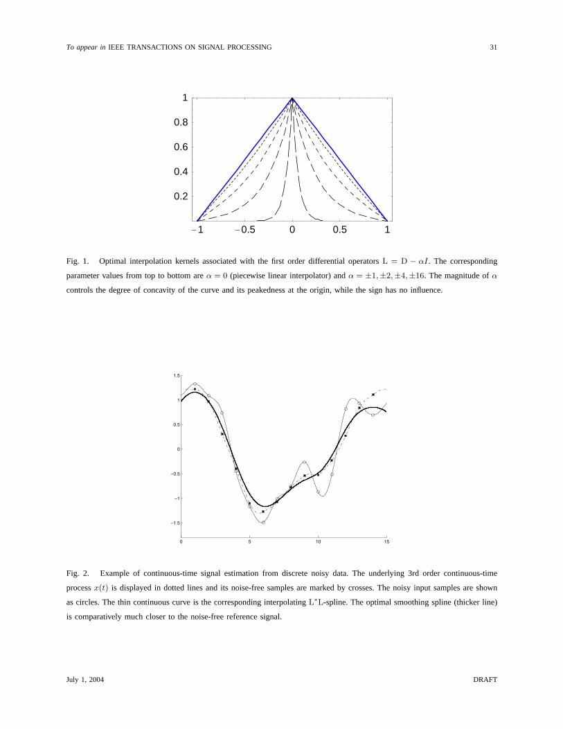
To appear inIEEE TRANSACTIONS ON SIGNAL PROCESSING 31
-1 -0.5 0 0.5 1
0.2
0.4
0.6
0.8
1
Fig. 1. Optimal interpolation kernels associated with the first order differential operatorsL = D − αI. The corresponding
parameter values from top to bottom areα = 0 (piecewise linear interpolator) andα = ±1,±2,±4,±16. The magnitude ofα
controls the degree of concavity of the curve and its peakedness at the origin, while the sign has no influence.
0 5 10 15
−1.5
−1
−0.5
0
0.5
1
1.5
Fig. 2. Example of continuous-time signal estimation from discrete noisy data. The underlying 3rd order continuous-time
processx(t) is displayed in dotted lines and its noise-free samples are marked by crosses. The noisy input samples are shown
as circles. The thin continuous curve is the corresponding interpolatingL∗L-spline. The optimal smoothing spline (thicker line)
is comparatively much closer to the noise-free reference signal.
July 1, 2004 DRAFT