•

•

o

•

GENERALIZED LINEAR MODELS IN BIOMEDICAL

STATISTICAL APPLICATIONS

byPranab Kumar Sen

Department of BiostatisticsUniversity of North Carolina

Institute of StatisticsMimeo Series No. 2152

December 1995

•

GENERALIZED LINEAR MODELS IN BIOMEDICAL STATISTICAL

APPLICATIONS+

PRANAB KUMAR SEN

University of North Carolina, Chapel Hill.

SUMMARY

In biological assays, clinical trials, life-testing problems, reliability and survival analysis, and a vari­ety of applied fields ranging from agrometry to biodivrersity to zodiacal sciences, generalized linearmodels covering usual linear, transformed linear, log-linear and nonlinear regression models, multi­nomial and logistic regression models, as well as some semiparametric ones, are potentially adoptablefor drawing statistical conclusions from acquired data sets. Yet there may be some hidden barriers,originating from experimental as well as observational schemes, that merit careful examination inapplications. Merits and demerits of generalized linear models in biomedical applications with dueemphasis on their validity and robustness properties are thoroughly discussed.

.. 1 INTRODUCTION

In a conventional experimental setup, the causal relationship of input and output variables isof prime interest, and such a picture is often smudged to a certain extent by chance fluctuationsor errors. To accomodate plausible chance variations around predictable or systematic levels, ina conventional linear model it is tacitly assumed that the output (or, dependent) variable, Y, isrelated to a set of explanatory (or, input) variables, x in a linear mode, subject to errors havingsome statistical (distributional) structures. For example, in a classical setup, it is assumed that

Y = f3'x+e, (1.1)

...

•

where f3 is an unknown vector of (regression) parameters, and the errors are generally assumedto have three basic properties: (i) normality (with zero mean and a finite variance (72), (ii) inde­pendence (for different observations) and (iii) homoscedasticity (at all levels of x). As a result,statistical analysis schemes pertaining to such linear models remain vulnerable to plausible depar­tures from linearity of the model as well as independence, homoscedasicity and normality of theerror components. The quest for studying robustness and validity of normal theory linear modelslaid down the foundation of more complex statistical models which may be used as alternative ones.Depending on a particular situation at hand, one or more of these basic regularity assumptions may

• AMS 1990 subject classifications: 62J12, 62N05, 62P99t Key words and phrases: Asymptotics; auxiliary variate; binning; bioassays: dilution, direct, indirect, parallel

line, qualitative, quantal, slope ratio; canonical link; censoring; clinical trials; competing risks; concomitant variate;conditional model; correlated binary responses; dosage; frailty models; GEE; hazard; isotonic regression; link function;logit; log-linear model; marginal analysis; measurement errors; misclassification; missing data; mixed GLM; multipleendpoints; NN-method; nonlinear model; nonparametrics; partial likelihood; Poisson regression; probit; PHM; quasi­likelihood; relative potency; response-metameter; risk; semi-parametrics; smoothing; step down procedure; time­dependent coefficients.

1

need special scrutiny, and that may dictate particular alternative models and appropriate statisticalanalysis procedures. Since in diverse fields of applications, the setups may vary considerably, it maybe more appropriate to consider some typical scenarios arising in some typical contexts, examine thedrawbacks of the classical linear model approach, and to introduce alternative models which mayhave greater appeal on the grounds of robustness and validity. Generalized linear models (GLM)are important members of this bigger class, and they are therefore to be examined with due care,relevance and importance.

Our perception ofGLM's is posed from a wider perspective than in NeIder and Wedderburn (1972)who showed how linearity in common statistical models could be exploited to extend classical lin­ear models to more gener;lJ ones and exact statistical inference tools can therefore be used. Fur­ther significant developments in this direction are reported in a unified manner in McCullagh andNeIder (1989). It follows from the current state of developments in this field that GLM's include,as special cases, linear regression and analysis of variance (ANOVA) models, log-linear models forcategorical data, product multinomial response models, logit and probit (or normit) models in quantalbio-assays, and some simple semi-parametric models arising in reliability and survival analysis. Inan exact treatise of the subject matter, GLM's pertain to a somewhat narrow class of statisticalproblems (where the relevance of the classical exponential family of densities can be justified). How­ever, with the widening impact of computers and large scale data analyses in every sphere of lifeand science, there is a genuine need to look into the prospects from a large sample perspective withdue emphasis on computational complexities as well as robustness properties. Our motivations inthe current study are primarily driven by such undercurrents.

In Section 2, we provide a brief outline of the basic GLM (exact) methodology which permits acomprehensive access to the large sample counterpart, which is reported in Section 3. GLM's role inanalysis of binary data with special emphasis on quantal bioassays is appraised in Section 4. Directdilution assays are introduced in Section 5, and the case of quantitative indirect assays is presentedin Section 6. The relevance of GLM's to nonlinear regression models is studied in Section 7 from alarge sample view point, while the case of nonparametric regression is considered in Section 8. Theconcluding section deals with a broad review of the scope and limitations of GLM's in applicationsin a wider perspective.

2 GLM: EXACT METHODOLOGY

The genesis of GLM lies in the exponential family of densities. Let Y1 , ... , Yn be independent(but not necessarily identically distributed) random variables, and assume that Yi has the densityfunction

..

j;(y;O;,</J) = c(y,O,</J)erp[{yO; -b(O;)}/a(</J)]' i= 1, ... ,n, (2.1)

where the 0; are the parameters of interest, </J(> 0) is a nuisance (scale) parameter, and a(·), b(·)and c(·) are functions of known forms. It is tacitly assumed that b(0) is twice (continuously) differ­entiable (with respect to 0 ), and we denote the first and second order derivatives by b' (.) and b" (.)respectively. Then, it is easy to check that

1-1; = EYi = 1-1;(0;) = b'(O;); VarYi = a(</J)b"(O;), i = 1, ... , n.

The last equation permits us to introduce the so called variance function v;{l-I; (O;)} by letting

{)v;{I-I;(O;)} = {)O/;(Od,

(2.2)

(2.3)

and it depends solely on 1-1; (Oi), for i = 1, ... , n. The 1-1; (Oi) play a basic role in the formulation ofGLM's. As we have assumed that the form of b(O;) is the same for all i, we have the form of 1-1;

2

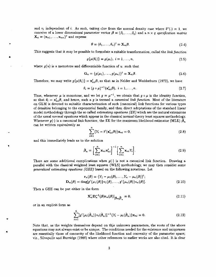
and Vi independent of i. As such, taking clue from the normal density case where b"(.) = 1, weconceive of a lower dimensional parameter vector {3 = ({31, ... , (3q) and a n x q specification matrixX n = (Xnl, ... ,xnnP and express

(2.4)

•This suggests that it may be possible to formulate a suitable transformation, called the link junction

(2.5)

where g(u) is a monotone and differentiable function of u. such that

(2.6)

Therefore, we may write g{J.I(Oi)} =x~i{3, so that as in NeIder and Wedderburn (1972), we have

(2.7)

Thus, whenever Jl is monotone, and we let 9 = Jl- 1, we obtain that 9 0 Jl is the identity function,so that Oi = x~i{3, and hence, such a 9 is termed a canonical link junction. Most of the literatureon GLM is devoted to suitable characterization of such (canonical) link functions for various typesof densities belonging to the exponential family, and then direct adoptations of the standard linearmodel methodology through the so called estimating equations (EE) which are the natural extensionsof the usual normal equations which appear in the classical normal theory least squares methodology.Whenever g(.) is a canonical link function, the EE for the maximum likelihood estimator (MLE) i3ncan be written equivalently as

•

n

L)Yi - b'(X~i{3)}Xni = 0,i=1

and this immediately leads us to the solution

i3n = [txniX~i]-1 [txniYi].1=1 1=1

(2.8)

(2.9)

There are some additional complications when g(.) is not a canonical link function. Drawing aparallel with the classical weighted least squares (WLS) methodology, we may then consider somegeneralized estimating equations (GEE) based on the following notations. Let

rn({3) = {Yl - Jll ({3) , ... ,Yn - Jln({3)}t;

Dn({3) = diag[g'{Jld{3)}vd{3), ... ,g'{Jln({3)}Vn({3)].

Then a GEE can be put either in the form

or in an explicit form as

n

L[g'{Jli(i3n)}Vi(i3n)]-I{Yi - Jli(i3n)}Xni = o.i=1

(2.10)

(2.11)

(2.12)

Note that, as the weights themselves depend on thje unknown parameters, the roots of the aboveequations may not always exist or be unique. The conditions needed for the existence and uniquenessare essentially those of concavity of the likelihood function and convexity of the parameter space;viz., Silvapulle and Burridge (1986) where other references to earlier works are also cited. It is clear

3

that in general we have implicit equations for the unknown {3, and in this way the analogy with theusual MLE may also be pointed out. We may note further that if the response is multivariate thenthere are additional complications in the formulation of link functions and variance-covariance func­tions. It may be difficult to find out canonical links (and even so, they may not be coordinatewisefunctions), and the variance-covariances may also be highly involved. For some important cases ofGLMs, we will discuss these aspects of the GLM briefly in later sections.

3 GLM ASYMPTOTICS

With respect to general asymptotics, the GLM may generally encounter more complications thanthe classical LSE or MLE. While the main complication arises due to the implicit nature of the GEE,it is further aggravated by the complexities of the link and variance functions. We follow the generalprescriptions in Sen and Singer (1993, sec. 7.4) in summarizing the general results depending on theunderlying structure in the form of the following three models.

(1) Model I. This relates to (2.1) when the basic random variables Yi are independent and nis large. A classical example is the Poisson regression model where the Yi are independent Poissonvariables with means Ai, and either the Ai or their logarithms are related linearly to a set of ex­planatory variables (vectors) Xi by means of a finite dimensional parameter vector {3j in this setupthe sample size n is assumed to be large. In terms of (3 the log-likelihood function for the model(2.1) is given by

n

In Ln({3) = ~)Yih(X~i{3) - b{h(x~i{3)}] + constant,i=l

where the constant term does not involve (3 and

h(·) = (g. J.t)-1 is /' and differentiable.

By some routine manipulations we derive the score statistic:

Un ({3) (8/8(3) In Ln ({3)n

= L {Yi - J.ti({3)} [9'{J.ti({3)}Vi({3)r 1Xni.i=l

Differentiating one more time with respect to {3 and taking expectation, we obtain

E{ - (82/8{38{3') In Ln ({3)}n

L {[g'{J.ti((3)}]-2[Vi({3)]-1 }XniX~i'i=l

If we let

W2i({3) = J.t;({3){g" {J.ti ({3)}[g'{J.ti ({3)}]-2

bill {h(X~i(3)[g' {J.ti({3)}]{Vi({3)} -3}, i = 1, ... , n,

4

(3.1)

(3.2)

(3.3)

(3.4)

(3.5)

(3.6)

f

then under two compactness conditions on the Wki{/3), k = 1,2; i = 1, ... , n, it follows from Theorem7.4.1 of Sen and Singer (1993) that for i3n' the MLE of {3 under this GLM, as n increases,

(3.7)

•Note that the observed second-deivative matrix of the log-likelihood function can be expressed asequal to In ({3) plus a remainder term Rn ({3) (matrix)[ see Sen and Singer (1993), p.307 ] whichhas a more complicated form than in the usual likelihood function case. This feature calls for theincorporation of suitable compactness conditions under which this remainder matrix can be handledadequately. For an alternative derivation of the asymptotic normality (and consistency) of MLE inGLS's, we may refer to Fahrmeir and Kaufmann (1985). Compared to the level of complexities intheir proof, the derivation in Sen and Singer (1993) based on the compactness conditions appears tobe simpler, and more akin to the classical MLE case. Moreover, such compactness conditions followfrom the natural continuity properties of the parametric functions in the exponential family, and arenot that difficult to verify in other specific cases not belonging to this family. Hence we advocatethe use of this compactness condition based approach.

(2) Model II. There are situations where the basic random variables Y; are themselves basedon suitable subsamples of sizes (say) ni (which may not be all equal). A handy example is theclassical logistic regression model where for each i(= 1, ... , k), for some fixed k(? 1), Y; relates tothe observed failure (or response) rates corresponding to a given combination of dose levels. Thus thenjY; are independent Bin(ni, 1l"i) variables where the 1l"i can be expressed in terms of a deterministicfunction of the dose levels. In logistic regression, we express

1l"j = {I + exp(-{3/Xi)} -1, for i = 1, ... , k,

so that for the logits we have

Bi =log{1l"i!(I-1l"i)} = {3/Xi, fori= I, ... ,k.

(3.8)

(3.9)

Usually in this setup, k is prefixed, while for each dose level, a number of subjects are administered,and guided by the convergence of the binomial law (appropriately normalized) to a normal law, itmay be assumed that there exist suitable normalizing factors, say, ani(Bd and bni(Bi )(> 0), suchthat for large values of ni,

{Y; - ani (Bi)} jbni(Bd -+D N(O, 1), 'v'i(= 1, ... , k). (3.10)

•

Thus whenever the GLM can be adopted for the Bi, using the conjugate transformation on the Y;and the aforesaid normality result standard large sample methodology can be incorporated to studythe asymptotic properties of the MLE of {3. We will discuss this in detail in a later section. Inpassing we may note that allowing k to be large in this setup does not create any additional compli­cations; rather it accelerates the rate of convergence to asymptotic normality and thereby facilitatesthe adoptation of the standard large sample methodology.

(3) Model III. This relates to the so called quasi-likelihood or quasi-score estimating equations,introduced by Wedderburn (1974). In this setup no specific assumptions are made concerning theform of the density in (2.1); it is assumed on the contrary that (i) the E(Y;) = Pi satisfy the GLMsetup, and (ii) Var(Y;) = (7"2V(Pi) where (7"2 is a possibly unknown positive scale function while theVi (.) are completely known variance functions. The related estimating equations may be posed as

• n

:L(8j8{3)p;{Vi(J.!i)}-1(y; - J.!i) = O.i=l

5

(3.11)

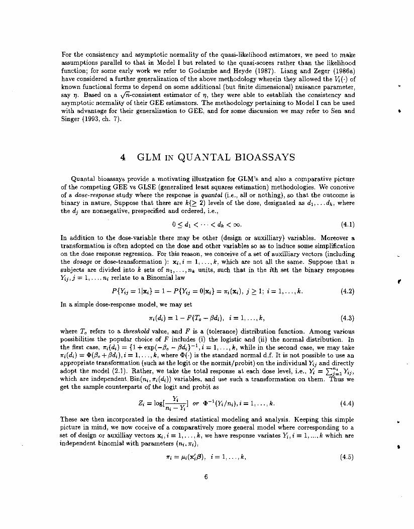
For the consistency and asymptotic normality of the quasi-likelihood estimators, we need to makeassumptions parallel to that in Model I but related to the quasi-scores rather than the likelihoodfunction; for some early work we refer to Godambe and Heyde (1987). Liang and Zeger (1986a)have considered a further generalization of the above methodology wherein they allowed the V; (.) ofknown functional forms to depend on some additional (but finite dimensional) nuisance parameter,say TJ. Based on a yin-consistent estimator of TJ, they were able to establish the consistency andasymptotic normality of their GEE estimators. The methodology pertaining to Model I can be usedwith advantage for their generalization to GEE, and for some discussion we may refer to Sen andSinger (1993, ch. 7).

4 GLM IN QUANTAL BIOASSAYS

Quantal bioassays provide a motivating illustration for GLM's and also a comparative pictureof the competing GEE vs GLSE (generalized least squares estimation) methodologies. We conceiveof a dose-response study where the response is quantal (i.e., all or nothing), so that the outcome isbinary in nature, Suppose that there are k(~ 2) levels of the dose, designated as d1 , ..• dk , wherethe dj are nonnegative, prespecified and ordered, i.e.,

In addition to the dose-variable there may be other (design or auxilliary) variables. Moreover atransformation is often adopted on the dose and other variables so as to induce some simplificationon the dose response regression. For this reason, we conceive of a set of auxilliary vectors (includingthe dosage or dose-transformation): Xi, i = 1, ... , k, which are not all the same. Suppose that nsubjects are divided into k sets of n1, ... ,nk units, such that in the ith set the binary responsesYij , j = 1, ... , ni rerlate to a Binomial law

P{Y'ij =1!Xi} =1- P{Y'ij =OIXi} =1I"i(Xi) , j 2: 1; i =1, ... , k.

In a simple dose-response model, we may set

1I"i(di ) = 1 - F(To - (3d;), i = 1, ... , k,

(4.1)

(4.2)

(4.3)

t

where To refers to a threshold value, and F is a (tolerance) distribution function. Among variouspossibilities the popular choice of F includes (i) the logistic and (ii) the normal distribution. Inthe first case, 1I"i (di ) = {1 + exp( - (3o - {3d;} -1, i = 1, ... , k, while in the second case, we may take1I"i(di ) = iP({3o + (3di ), i = 1, ... , k, where iP(.) is the standard normal d.f. It is not possible to use anappropriate transformation (such as the logit or the normit/probit) on the individual Yij and directlyadopt the model (2.1). Rather, we take the total response at each dose level, i.e., Yi = Lj~l Yij,which are independent Bin(ni,1I"i(di )) variables, and use such a transformation on them. Thus weget the sample counterparts of the logit and probit as

Zi =log[ni ~ Yi] or iP- 1(Yi/ni), i = 1, ... , k. (4.4)

These are then incorporated in the desired statistical modeling and analysis. Keeping this simplepicture in mind, we now coceive of a comparatively more general model where corresponding to aset of design or auxilliay vectors Xi, i =1, ... , k, we have response variates Yi, i = 1, ... , k which areindependent binomial with parameters (ni, 1I"i),

..

•1I"i=JLi(xi,8), i=1, ... ,k,

6

(4.5)

and the functional forms of the J.li(.) are assumed to be known. Finney (1978) contains an excellentaccount of statistical methodology of the probit model, while the logit model has been extensivelystudied in the literature, mostly in the context of log-linear models for categorical data; we mayrefer, for example, to Sen and Singer (1993, ch.6 -7), where other pertinent references are also cited.

•In this formulation we can directly link the methodology presented in Section 2 and carry out the

appropriate statistical analysis by reference to the GLM methodolgy described therein. The mainpoint of departure is, however, the basic fact that the Yi are not the elemetary variables but arecomposed from them for each bucket separately. This makes the variance V ar(Yi) dependent notonly on the known scale factor nil but also on the unknown {3 through the 1I";{1 - 11";} which areof more complex nature. This feature calls for appropriate asymptotic tools for providing suitableapproximations for the GEE and the derived MLE, and we will pay due attention to this development.

In view of the comment made above it seems that in this case we may not be able to make useof the estimating equation in (2.8), and we have to incorporate the GEE in (2.12) for obtaining theMLE /3 of (3. This calls for an iterative procedure in which we start with an initial (consistent)

estimator /3(0), estimate the variance function in (2.12), and using the scoring procedure outlined inSection 3, we can obtain the first-step estimator of {3 as well as the variance function. We can iteratethis procedure a number of times, and for a suitable choice of r (usually 2 or 3), we may use anr-step procedure to approximate the MLE adequately. It is clear that in this iteration scheme thereare certain elements of asymptotic theory which merit a careful study. First, if we use the logit,probit (or any other nonlinear transformation) on the Yi, the computation of the exact variance ofthe transformed variate may run into complexities. For this reason in the logistic regression modelwe start with an estimating equation:

k

Qn(l30,{3) = L:Pi(l- Pi)ni[Zi - 130 - {3'Xi]2,i=l

(4.6)

(4.7)where

PiZi = log[--], Pi = Yifni' for i = 1, ... , k.1- Pi

The basic difference between this estimating equation and the GEE in (2.12) (for a logit transforma­tion) is that here we use p;(1 - Pi) ni as an estimate of the reciprocal of the (asymptotic) variance ofZi, so that the weighted least squares estimation theory can directly be adopted for the estimation of130 and (3. On the other hand, the difference between the variance function in (2.12) and niPi(l- Pi)can be shown to be Op(n;1/2), so that this approximation does not entail any significant discripancywith the MLE derived from (2.12). In that sense, the GEE is a minor refinefent over the logisticregression approach when the individual sample sizes n1, ... ,nk are all large. If these sample sizesare not large, the expression for the variance functions in (2.12) may not retain their exactness, andhence the rationality of the GEE in (2.12) may not be that clear. The situation with the Probitanalysis is a bit more complex (see, for example, Finney 1978) where the estimating equations aremore complex and so are the corresponding variance functions. Nevertheless, the iterative procedurewith the GEE works out well for large sample sizes. The question remains open: How large shouldbe the sample sizes in order that the asymptotics in GEE are adequate? Second, from the asymp­totics point of view, we are basically in Model II of Section 3, where the emphasis on GEE entailsmuch less of the GLM than the appropriateness of the transformation and its asymptotic normalproperties. Thus, the primary force behind GLM is somewhat imperceptible in this asymptoticcase. Finally, the GLM may entail a comparatively severe nonrobustness feature than some otheralternative models. For example, suppose that the true tolerance distribution is F and we assumea logistic model. Then, if the XI are so chosen that the resullting 1I"i are not all clustered around0.5, the estimator of {3 based on this logit model may be highly nonrobust to plausible departure of

t

...

•

7

F from a logistic distribution, A similar feature is shared by the probit model. Another importantcase relates to a mixture model in quantal response where a GLM approach has been consideredby Cox (1992), and this also reveals the nonrobustness aspects of the conventional methodology. Inactual applications this robustness feature therefore merits due considerations.

5 GLM IN DIRECT DILUTION ASSAYS

In bioassay, typically, a new (test) and a standard preparation are compared by means of reactionsthat follow their applications to some some subjects, and the relative potency of the test preparationwith respect to the standard one is the focal point of the study. In a direct assay, the dose of a givenpreparation needed to produce a specified response is recorded, so that the dose is a nonnegativerandom variable (r.v.) while the response is certain. Consider a typical direct bioassay involvinga standard preparation (S) and a test preparation (T). Suppose that the standard preparationis administered to m subjects, and let Xl, ... , Xm be the respective doses to yield the desiredresponse. Thus we assume that the Xi are independent and identically distributed (i.i.d.) r.v.'swith a distribution function (d.f.) Fs defined on n+ = [0,00). Similarly, let Yl , ... , Yn be the dosesfor the n subjects on which the test preparation has been administered; these are assumed to bei.i.d.r.v. with a d.f. FT defined on n+. In many cases we may think that the test preparationbehaves, in a properly interpreted bioequivalence setup, as if it is a dilution (or concentration) of thestandard one. Under this hypothesis, we have

..

FT(X) =Fs(px), 'Vx E n+, where p > O. (5.1)

Then p is termed the relative potency of the test preparation with respect to the standard one, and(5.1) constitutes the fundamental assumption in a direct (-dilution) assay; we refer to Finney (1978)for an excellent coverage of this subject matter in a strict parametric setup where the F are mostlyassumed to be normal or log-normal d.f.'s. The very assumption that Fs is normal may run intoconceptual obstructions unless the mean of this d.£. is sufficiently large compared to its standarddeviation so that Fs(O) can be taken to be equal to O. Moreover, in actual practice, these tolerarancedistributions are usually highly positively skewed, and hence suitable transformations on the dose(called the dosage) are generally recommened to induce more symmetry of the d.f. of the trans­formed variable. Among these, two popular ones are the foolwing:

(i) log-dose transformation: X· =log X.(ii) Power transformation: X· = X>.., for some .A > O. Typically, .A is chosen to be

1/2 or 1/3 depending on the nature of the dose.

If we work with the model (5.1) we have a typical scale-model, so that standard MLE of p canbe obtained under normality assumptions; note in this respect that the variances of Fs and FTare not equal (unless p = 1), but their coefficients of variation are equal. In the case of log-dosetransformation, we have a standard two-sample model (with equal variances), so that GLM remainshighly pertrinent. In the case of power-dose, the choice of.A is crucial, and moreover the homogeneityof the variances of the dosages may not be taken for granted, unless p = 1. In this respect, thereappears to be some ambiguity in Finney (1978) and other text books on bioassays where often thewell known Fieller theorem (on the ratio of two means) has been adopted without proper safeguard.This technical difficulty does not arise in the case of log-dose transformation, but the resulting MLE(of p) becomes highly sensitive to the assumed normality. In a variety of situations the log-dosetransformation induces a greater amount of symmetry to the original the d.f., but still it may not befully symmetric, or even so, may differ from a normal d.f., often quite remarkably. Thus, in using the

8

•

..

•

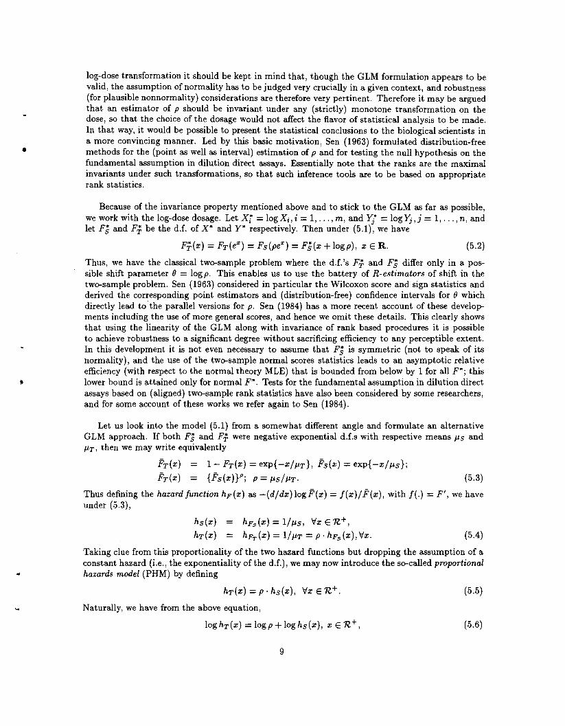
log-dose transformation it should be kept in mind that, though the GLM formulation appears to bevalid, the assumption of normality has to be judged very crucially in a given context, and robustness(for plausible nonnormality) considerations are therefore very pertinent. Therefore it may be arguedthat an estimator of p should be invariant under any (strictly) monotone transformation on thedose, so that the choice of the dosage would not affect the flavor of statistical analysis to be made.In that way, it would be possible to present the statistical conclusions to the biological scientists ina more convincing manner. Led by this basic motivation, Sen (1963) formulated distribution-freemethods for the (point as well as interval) estimation of p and for testing the null hypothesis on thefundamental assumption in dilution direct assays. Essentially note that the ranks are the maximalinvariants under such transformations, so that such inference tools are to be based on appropriaterank statistics.

Because of the invariance property mentioned above and to stick to the GLM as far as possible,we work with the log-dose dosage. Let Xi =log Xi, i =1, ... , m, and ~. =10gYj,j = 1, ... , n, andlet Fsand F;; be the dJ. of X* and Y* respectively. Then under (5.1), we have

(5.2)

"

Thus, we have the classical two-sample problem where the d.f. 's F;; and Fs differ only in a pos­sible shift parameter B = log p. This enables us to use the battery of R-estimators of shift in thetwo-sample problem. Sen (1963) considered in particular the Wilcoxon score and sign statistics andderived the corresponding point estimators and (distribution-free) confidence intervals for B whichdirectly lead to·the parallel versions for p. Sen (1984) has a more recent account of these develop­ments including the use of more general scores, and hence we omit these details. This clearly showsthat using the linearity of the GLM along with invariance of rank based procedures it is possibleto achieve robustness to a significant degree without sacrificing efficiency to any perceptible extent.In this development it is not even necessary to assume that Fs is symmetric (not to speak of itsnormality), and the use of the two-sample normal scores statistics leads to an asymptotic relativeefficiency (with respect to the normal theory MLE) that is bounded from below by 1 for all F*; thislower bound is attained only for normal F*. Tests for the fundamental assumption in dilution directassays based on (aligned) two-sample rank statistics have also been considered by some researchers,and for some account of these works we refer again to Sen (1984).

Let us look into the model (5.1) from a somewhat different angle and formulate an alternativeGLM approach. If both Fs and F;; were negative exponential d.f.s with respective means J.ts andJ.tT, then we may write equivalently

FT(X) = 1 - FT(X) =exp{-xlJ.tT}, Fs(x) =exp{-xlJ.ts};

FT(X) {Fs(x)}P; p = J.tSIJ.tT. (5.3)

Thus defining the hazard function hF(x) as -(dldx) logF(x) = f(x)IF(x), with f(.) =F' , we haveunder (5.3),

hs(x) =hT(X)

hFs(x) = 1/J.ts, 'ix E'R+,

hFT(X) = 1/J.tT = p. hFs(X), 'ix. (5.4)

Taking clue from this proportionality of the two hazard functions but dropping the assumption of aconstant hazard (i.e., the exponentiality of the d.f.), we may now introduce the so-called proportionalhazards model (PHM) by defining

hT(X) = p. hs(x), 'ix E 'R+.

Naturally, we have from the above equation,

loghT(x) = logp + loghs(x), x E 'R+,

9

(5.5)

(5.6)

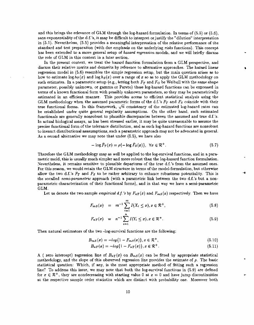
and this brings the relevance ofGLM through the log-hazard formulation. In terms of (5.5) or (5.6),sans exponentiality of the d.f. 's, it may be difficult to interpret or justify the" dilution" interpretationin (5.1). Nevertheless, (5.5) provides a meaningful interpretation of the relative performance of thestandard and test preparation (with due emphasis on the underlying risks functions). This concepthas been extended to a more general setup of hazard regression models, and we will briefly discussthe role of GLM in this context in a later section.

In the present context, we treat the hazard function formulation from a GLM perspective, anddiscuss their relative merits and demerits by reference to alternative approaches. The hazard linearregression model in (5.6) resembles the simple regression setup, but the main question arises as tohow to estimate log hT (x) and log hs (x) over a range of x so as to apply the GLM methodology onsuch estimates. In a parametric setup (e.g., letting both FT and FG be Weibull with the same shapeparameter, possibly unknown, or gamma or Pareto) these log-hazard functions can be expressed interms of a known functional form with possibly unknown parameters, so they may be parametricallyestimated in an efficient manner. This provides access to efficient statistical analysis using theGLM methodology when the assumed parametric forms of the d.f.'s FT and Fs coincide with theirtrue functional forms. In this framework, vn consistency of the estimated log-hazard rates canbe established under quite general regularity assumptions. On the other hand, such estimatedfunctionals are generally nonrobust to plausible discrepancies between the assumed and true d.f. 'soIn actual biological assays, as has been stressed earlier, it may be quite unreasonable to assume theprecise functional form of the tolerance distribution, and as such log-hazard functions are nonrobustto ineaxct distributional asasumptions, such a parametric approach may not be advocated in general.As a second alternative we may note that under (5.5), we have also

•

-logFT(x) = p{-logFs(x)}, "Ix E n+. (5.7)

Therefore the GLM methodology may as well be applied to the log-survival functions, and in a para­metric mold, this is usually much simpler and more robust than the log-hazard function formulation.Nevertheless, it remains sensitive to plausible departures of the true d.f. 's from the assumed ones.For this reason, we would retain the GLM structure in terms ofthe model-formulation, but otherwiseallow the two d.f. 's FT and Fs to be rather arbitrary to enhance robustness potentiality. This isthe socalled semi-parametric approach (with a parametric link between the two d.f.'s but a non­parametric characterization of their functional forms), and in that way we have a semi-parametricGLM.

Let us denote the two sample empirical d.j. 's by FnT(X) and Fms(x) respectively. Then we have

m

m- 1 L:I(X;:S x),x E n+,;=1n

n- 1 L:I(Yi:S x),x E n+.;=1

(5.8)

(5.9)

Then natural estimators of the two -log-survival functions are the following:

Bms(x) =-log{1- Fms(x)},x E n+,BnT(X) = -log{1 - FnT (x)} , x E n+.

(5.10)

(5.11)

A ( zero intercept) regression line of BnT(X) on Bms(x) can be fitted by appropriate statisticalmethodology, and the slope of this obsrerved regression line provides the estimate of p. The basicstatistical question: Which, if any, is the most appropriate method of fitting such a regressionline? To address this issue, we may note that both the log-survival functions in (5.9) are definedfor x E n+, they are nondecreasing with starting value 0 at x = 0 and have jump discontinuitiesat the respective sample order statistics which are distinct with probability one. Moreover both

10

..

....

are stochastic, so that we have a case where the dependent as well as the independent varriates(functions) are subject to errors. We introduce two empirical processes {wJ;) (x), x E n+} and{WA2 )(x), x E n+} as follows:

WJ.l) (x) =wJ2)(x)

[Bms (x) + logFs(x)], x E n+,[BnT(x) + logFT(x)], x E n+. (5.12)

f Borrowing the reverse martingale (process) characterization of the empirical d.f. (with respect tothe index m (or n) ) and noting that -log(1 - y) is a convex function of y E (0,1), we claim as inSen (1973) that both the empirical processes defined by (5.10) are reverse submartingale processes(with respect to the sample size sequences) and that they are independent. Although such charac­terizations enable us to propose some ad hoc estimators of p, they do not lend to any simple (andyet efficient) solution.

There appears to be a rather simple approach based on the conventional Q-Q plot. Note thatunder the proportional hazard assumption,

Keeping this identity in mind, we may introduce the sample functions

Zm,n(P) = log{FnT(F,;;1(p))}, p E (0,1).

(5.13)

(5.14)

At any specific value of p : 0 < p < 1, Zm,n(p)/{logp} is a consistent estimator of p. Thereforehomogeneity of such pointwise estimates (over a set of points inside (0,1)) conforms to the adequacyof the proportional hazard model, and then these may be pooled to obtain an efficient estimator ofp. In this context the choice of a set of gridpoints (for p ) or p in continuum in a compact subintervalof (0, 1) merits a careful study, and the related asymptotic theory is planned to be considered in asubsequent communication.

6 GLM IN INDIRECT QUANTITATIVE ASSAYS

In an indirect quantitative assay, doses at several levels are prescribed to several subjects, andtheir responses, quantitative in nature, are recorded. Therefore, for a spefified dose, say, d(> 0), thestochastic response, say, Yd follows a d.f., say, Fd(X), and an average (mean, median or someothermeasure of the central tendency) define a dose-response regression. Generally, this regression lineis nonlinear, and suitable transformations on the dose and/or response variates are made to reducethis sensibly to a linear form. Such transformations are termed the dosage ( or dose-metameter) andresponse-metameter. In a parametric ananysis, it is therefore assumed that the response-metameterhas a linear regression on the dosage with a distribution of the errors of a specified form (involvingsome unknown parameters). Standard parametric procedures are then usually employed to esti­mate the parameters appearing in the regression form as well as the nuisance parameters associatedwith the tolerance d.f. 'so Under the basic assumptions that the underlying d.f.'s are all (homoscedas­tic) normal laws, detailed statistical analysis schemes and their properties are given in Finney (1978).

Parametric models based on transformations on the dose/response variates and a spefified form ofthe tolerance distribution brings the direct relevance ofthe GLM, particularly, when this distributionbelongs to the exponential family for which the exact GLM methodology sketched in Section 2

11

remains adoptable. In that set up, we may therefore claim some optimality properties of suchGLM based solutions. Thus under the normality assumption, the normal theory model and analysisschemes considered in detail in Finney (1978) are very appropriate from statistical point of view. Inthe framework of earlier sections, we suppose that a standard and a test preparation are administeredto a set of subjects, and we conceive of linear dose-response regressions along with a specifiedfunctional form of the error d.f. which involves only a finite number of nuisance parameters. Thesetwo dose-response regression lines are denoted by

Ys =as + f3sx + es and YT =aT + f3Tx + eT· (6.1),

There are two popular models of indirect assays: (i) parallel line assays and (ii) slope ratio assays.The former arises commonly when a logarithmic transformation is used, while the other one is at­tuned to power-type transformations.

In a parallel line assay, the two regression lines are conceived to be parallel, so that we have thatboth es and eT have a common d.f., and moreover

135 = f3T = 13 (unknown); aT - as = 13 log p, (6.2)

where p(> 0) is the relative potency of the test preparation with respect to the standard one. (6.2) isreferred to as the fundamental assumption in this parallel line assay. Note that for the estimation ofthe common 13, we can adopt the standard linear model approach based on the classical least squaresestimators, and this is optimal when the error distributions are assumed to be normal. The situationwith p is somewhat different. Note that log p can be expressed as the ratio {aT - as} /13, so thatthe least squares estimators of these three parameters can be used to yield a point estimaor. Butwhen it comes to derive a suitable confidence interval for (log)p, we encounter the problem of havingan estimator of two statistics which are both linear (and normally distributed under normality ofthe errors). Asymptotically these two estimators are normal when properly standardized, so that asimilar problem arises in the estimation of the standard error of log p or in attaching a confidenceinterval for the parameter logp. In this context, the classical Fieller's theorem is generally adoptedin a parametric setup. This is clear from the above discussion that such estimation procedures aregenerally nonrobust to possible departures from the assumed normality of the errors. Moreover gen­erally the estimating equations are complex. However, allowing possible differences in the dose levelsfor the test and standard preparations and choosing a geometric progression for each, we obtain anequispaced desig npoints for the dosage, and in this sense, symmetric 2k-points designs are popularand convenient for such assays. Since the dosage levels span suitable ranges, the issue of robustnessmerits a careful examination. Robust and nonparametric methods are therefore appealing in thisrespect. Sen (1971) considered some simple robust estimation and testing procedures for such par­allelline assays, and these are further reviewed in Sen (1984).

The situation is somewhat different for the slope ratio assay. In such a case, referred to thelinearized dose-response regression mentioned before, we have

f

aT = as = 0: (unknown) and f3T = /'f3s, (6.3)

where>.. > O. Moreover, in this case, the two errors es and eT may not have the same distributioneven if they are normal. Thus, the homoscedasticity condition does not hold (unless p = 1). Notethat here the equality of the intercept parameters aT, 0:5 constitutes the fundamental assumption,and p = {f3T / f3s pi>' is nonlinear even if>" is specified. For this reason in attaching a confidence inter­val for the relative potency or even estimating the standard error of the estimated p, there may notbe an optimal procedure, even asymptotically. Fieller's theorem can be used with some advantage,but there is no guarantee that the roots are both real. In this setup because of the common interceptit is customary to have a (2k + I)-point design, and standard normal theory analysis schemes are

12

•

•

,

reported in detail in Finney (1978). Scope for vulnerability to non-normality and heteroscedasticityof the two error distributions is even more in slope ratio than in parallel line assays, and hence, anunconditional surrender to the standard GLM methodology is not advocated. Sen (1972a,b) containthe methodological development of suitable robust and nonparamteric inference procedures whichretain the basic GLM structure sans the normality or other specific forms of the error distributions;these were further unified in Sen (1984). We therefore skip these details.

In the preceding section, we have briefly outlined the PHM arising in direct dilution assays.Such PHM can also be imported for the indeirect assays discussed above. If we assume that boththe response distributions, (for the test and standard preparations) are absolutely continuous sothat their hazard functions hT(ylx) and hS(Ylx), corresponding to a dosage level x, are definedappropriately for dosage x belonging to a domain X, then treating the dosage levels as designvariates (i.e., nonstochastic), we may formulate a PHM as in Cox (1972). We consider an arbitrary(baseline) continuous, nongegative hazard function ho(y), y E Y and express

hs(Ylx) ho(y) . exp{as + f3sx},

hT(ylx) ho(y) . exp{aT + f3rx}, (6.4)

for x E X, y E y. Note that in (6.4) if we work with the log-hazard functions we end up witha parametric linear regression part and a nonparametric component i.e., log ho (y) which does notdepend on the concomitant variate(s). In this setup, it is also possible to introduce other designvariables as concomitant ones, so that x may as well be taken as a vector and the corresponding f3'sare to be taken' as vector too. This formulation allows us to treat the baseline hazard function asarbitrary while the effects of the design variates and the test vs. standard (i.e., treatment) variateare taken as covariates in a simple parametric structure. For example, in a parallel line assay wemay as before take the regression slopes to be equal and define the (log-)relative potency as theratio of the difference of the intercepts and the common slope. A similar formulation can be madefor the slope ratio assay. That way the relative potency can be defined and interpreted in terms ofthe hazard-regression parameters (on the the covariates), treating the base line hazard as a nuisanceparameter (functional). This formulation paves the way for semi-parametric approaches to statis­tical modeling and analysis of indirect quantitative bioassays, and in a more sophisticated mannerappropriate counting processes with stochastic intensity functions can be incorporated to impartrefined statistical tools. We may refer to the recent encyclopedic volume by Andersen et al. (1993)for an extensive treatment of this subject matter. The intricate relationship between the GLM andPHM (or semi-parametric) approaches becomes quite apparent if we probe into the coreespondingestimating equations which resemble the GEE in a visible manner. The basic difference here is thenuisance parameter (functional) ho(y), y E Y which calls for a partial likelihood approach, and thisleads to some loss of information resulting in some sacrifice of efficiency. On the other hand, thisapproach lends itself in a natural way to random censoring schemes which may arise in practice dueto withdrawal or dropout of the subjects due to causes other than the failure or the primary end­point of the investigation, though the loss of efficacy can be quite severe under heavy censoring. Ofcourse, in such censored models, almost all the procedures used in practice are subject to the samedrawback, and hence, such a critisims should not be labelled to the PHM alone. Nevertheless, wetake this opportunity to point out also the nonrobustness aspects of such refined statistical modelingand analysis schemes.

It follows from (6.4) that for parallel line assays, under the PHM, for every x EX, y E Y,

hT(y I x)jhs(y I x) = exp{f31ogp} = p~ (6.5)

which does not depend on the level y. On the other hand, by the fundamental assumption of parallelline assays, we have

hT(y I x) f(y - aT - f3x)j F(y - aT - f3x)

13

f(y - O:s - j3x - j3logp)jF(y - O:s - j3x - j3 log p)

hs(y-j3logplx)' yEY, xEX. (6.6)

Therefore from the last two equations we conclude that in order that a PHM is appropriate to theparallel line assay model, we need that

hT(y Ix)jhs(Y Ix) =pf3 = hs(y - j3logp Ix)jhs(Y Ix),

for every x EX, Y E y. This in turn implies that

hs(y - j3logp Ix) = pf3 . hs(y Ix), \:Ix EX, y E y.

Therefore, we need to have

hs(y -loge Ix) =e· hs(y I x), \:Ie> 0, y E Y, x E X.

(6.7)

(6.8)

(6.9)

,

In view of the fact that in a parallel line assay we have usually a log-dose and log-response trans­formation, the domain Y is the entire real line, so that the last equation does not hold for mostof the common tolerance distribution. A similar picture holds for the slope ratio assay. Therefore,in order that a PHM is deemed appropriate in an indirect quantitative bioassay, we may have toforego the usual fumdamental assumptions of parallel line or slope ratio assays. Although alternativemodeling may be possible, that would require a different interpretation of relative potency (in termsof relative risks), and such a definition may also entail a dependence of this risk ratio on the levelof dosage. In clinical trials where such PHM's are commonly adopted, a basic requirement is thatthe two hazard functions do not cross each other, so that one survival function lies under the otherfor all y, x. Again this basic condition may not be generally true; we may refer to Sen (1994b) forsome illustrative examples. If our basic goal is to investigate the relative risks of a standard anda test preparation over a domain of the dosage, then more general nonparametric modeling can beadopted to achieve this goal, although this may entail a very large sample size requirement. We willdiscuss this later. But, the sensitivity of the PHM in this context to model departures is quite clearfrom the above discussion. Even a small departure can alter the statistical picture and invalidatethe derived conclusions to a greater extent.

7 GLM IN NONLINEAR MODELS

In the context of bioassays, we have seen that dose- and response-metameters often reduce thedose-response regression to a sensibly linear form, so that standard least squares theory or GLMcan be adapted with some success. From robustness considerations, however, there may be somegenuine concern about the distributional assumptions to be made and impact of their departuresfrom the true (unknown) situation. This problem is much more complex in a general nonlinearmodel, even when the nature of the function is assumed to be of a given form (involving someunknown parameters or algebraic constants). In such a setup, we assume that the response variateY is related to a set of auxiliary variables, designed by a vector x belonging to a suitable space X,by means of a stochastic model

•

Y =g(x) +f, X E X, (7.1)

where the error component f has a given distribution F involving possibly some unknown parameterswhile the form of the regression function g(.) is assumed to be given, although it may also involvesome unknown parameters. In this formulation we have a predominant parametric flavor. A semi­parametric formulation can be conceived of by rendering either the form of 9 to be arbitrary but F

14

•

to be given, or 9 to be of a given form but F is allowed to be arbitrary. A complete nonparametricmodeling relates to the situation where both 9 and F are arbitrary. The nature of the postulated 9thus adds a second layer of nonrobustness prospects to GLM based parametrics.

To link such nonlinear models to the bioassay models treated in earlier sections we consider againthe parallel line assays in a more general mold of nonlinear dose-response regression. We stick tothe same notations as far as possible. Thus, we assume that at a given dosage level x, the d.f. ofYT and Ys, denoted by FT and Fs respectvely, are given by

FT(ylx) =F(y - mT(x)), Fs(y) =F(y - ms(x)), y E Y (7.2)

where F has a specified functional form ( for example, normal, logistic, Laplace etc), and the tworegression functions mT(x) and ms(x), x E X are of given (nonlinear) forms, such that

mT(x) - ms(x) = Q*, \:j x E X. (7.3)

This two-sample model can be regarded as a particular case of a more general model wherein wemay introduce some other design (or dummy) variables (vectors) Ci, i = 1, ... , n, and for the ithresponse ~, we frame the regression model:

where the errors fi are assumed to be i.i.d.r.v.'s with a d.f. It may not always be wise to imposethis i.i.d. structure on the errors. Even in the case of simple linear models, heterscedasticity of theerrors may have a profound effect on the optimality properties of common statistical inference toolsand this can be more significant for GLMs; we refer to Carroll and Ruppert (1988) for some usefuldiscussions on this nonrobustness properties F of given form, and the functional forms of g1 and g2are also assumed to be given, all involving some unknown parameters. It is also possible to combineg1 and g2 into a more complex function g(c, x). In this context we may note that under the i.i.d.structure of the fj, we may consider the total sum of squares due to error:• n

L {~ - g1(C;) - g2(Xj)} 2,i=1

(7.4)

(7.5)

which for given ~, Cj, Xi, i = 1, ... , n becomes a function of the unknown parameters associatedwith the functional forms of g1 and g2. Thus minimizing the above norm with respect to theseunknown parameters, we obtain a set of estimating equations which lead to their generalized leastsquares estimators. Such estimators are linear in the ~, but not generally in the Cj or Xi, and hencemay be quite cumbersome to solve algeabraically. The situation may become even more complexwhen we combine the two functions g1,g2 into a single g(c,x). Moreover depending on the natureof such g's, the resulting LSE may be (often highly) nonrobust. Such nonrobustness arises due topossible departures from these assumed functional forms, and also from possible departures fromthe distributional assumption on the errors. In the literature usually such error distributions aretaken to be normal; that leads to the homoscedasticity condition as a by-product, and hence in theabove equation the unweighted sum of squares is justifiable. On the other hand, sans this normalityof the errors, the homoscedasticity condition can not be taken for granted, and hence the sensitivityof these LSE to possible heteroscedastisity of the errors remains of serious concern.

From the above discussion it appears that there is a genuine need for appropriate GLM method­ology that can be adopted for nonlinear models. The principal difficulty stems from the fact that forgeneral nonlinear models, particularly involving vector-valued auxiliary variables, finding an appro­priate link function may be hard, and the soultion for a canonical link function may even be harder.This puts the general GLM methodology in a rather ackward situation, and on the top of that

15

generally these estimastes share nonrobustness properties to a greater extent than in the simplercases treated in earlier sections. Quasi-likelihood estimators discussed in Section 3 [see (3.11)] havea better appeal in this case, but again their estimating equations may be too complex. Robustnessconcerns remain pertinent in this setup too. Judged from all these aspect we may conclude thatwhenever we have confidence in an assumed functional forms of the 9r, r = 1,2, but we are notso confident about the particular distributional assumption made on the errors, a semi-parametricapproach may work out better for large sample sizes. Of course, if the sample size is large enough,one may even go for a complete nonparametric soultion which will have better robustness proper­ties. We will discuss this aspect of semi-parametrics and nonparametrics in the next section, andhence, we avoid the repetition. Nevertheless, we may comment that for all such estimators, exact orfinite-sample properties are generally hard to study, and hence the exact sample properties of theGLM methodology are not tracable in such an asymptotic setup. Of course, the GEE methodolgyis more appropriate here in an asymptotic setup.

8 GLM AND NONPARAMETRIC REGRESSION

The basic attraction of GLM's is the scope of their exact (statistical) treatment through thechoice of appropriate link functions or other transformations. On the other hand such a choice usu­ally demand some specific parametric structures, and hence, it may be desirable to check whetheror not such parametric models are appropriate in the given context. For example, referring back tothe bioassay problems, say in the quantal response case, we may use a logit or probit model underthe assumption that the tolerance distribution is logistic or normal with a linear regression on thedosage. Thus not only we make specific distributional assumptions, but also assume linearity ofregression. This may open up the avenues for lack of robustness on both of these counts. As such, itmay be desirable to relax such stringent parametric conditions by less restrictive ones. Two specifictypes of models evolve in this connection:

(1) Nonparametric regression models. No specific parametric structure is imposed on the toler­ance distribution or the dose-response regression function.

(2) Semi-parametric regression models. Here for a part of the model, some parametric structureis taken for granted while for the complementary part a nonparametric modeling is adopted. Forexample, in the quantal bioassay model, we may assume that the tolerance distribution is logisticor normal, but the dose-response regression is arbitrary (possibly monotone and smooth in a welldefined sense). Alternatively, we may also take the tolerance distributions to be arbitrary (continu­ous) but the dose response regression to be of a specified parametric form. The classical Cox (1972)PHM also belongs to such semi-parametric family of models.

The choice of a semi-parametric or nonparametric regression model is largely governed by theconfidence of the experimenter on plausible parametric structures underlying the experimental setup.From robustness considerations it may be preferable to choose a nonparametric model rather than asemi-parametric one. On the other hand, the very generality of a nonparametric approach may leadto a so-called large parameter space or a functional (i.e., infinite-dimensional). parameter space, andwith the increase in the dimension of such parameter spaces, the precision of statistical conclusionsattainable in a finite sample rapidly goes down. Thus, generally, a nonparametric approach mayrequire a larger sample size to match the precision level attainable by a semi-parametric model,whenever the latter one is the true model. On the other hand, if the chosen model is not the trueone, a semi-parametric model may result in significant bias and this may tilt the picture in an op­posite direction.

16

..

••

..

It is not uncommon to have a set of auxiliary variables for which some parametric models mayappear reasonable, while there may be others for which a nonparametric one would be more appro­priate. For example, we may refer to the regression model in (7.4). Since there the design variablesCj are nonstochastic, with suitable transformations, a linear form for the regression function 9dcdmay appear to workable in some situations. On the other hand, for the stochastic variates Xj, sucha parametric regression function may not be that reasonable, and hence, we may prefer a completenonparametric form for the regression function 92(X). In conventional experimental designs, it isnot uncommon to have some "fixed-effects" parameters and some other as "random-effects" ones.For example, in animal studies, if the blocks are formed by common mothers, the block effects aretreated as random while the treatment effects are treated as fixed one. This results in a so-calledmixed-effects models. In a traditional setup, the random effects are assumed to have (joint) nor­mality with specific covariance-structures, and this allows one to use conventional normal theoryinference tools for drawing statistical conclusions. But all these assumptions require careful scrutinybefore one adopts such classical models in practice. The discussion made above pertains to GLM aswell. In a GLM we may accept the GL part to a certain extent, and yet may not like to make specificdistributional assumptions, so as to make our conclusions more robust to plausible departures fromconventioal parametric models. To illustrate this point, we refer to the PHM treated in (5.4)-(5.6).We deal with this model in a more general manner by incorporating nonstochastic design variates Cjand stochastic concomitant variates Xj along with the primary response variate Yi, for i = 1, ... , n.Let f(ylc, x) be the conditional density of Y, given c, x, and the corresponding conditional hazardfunction be denoted by h(ylc, x), y E Y, c E 'R.P, x E nq , p, q ~ O. In a PHM we set

where ho(y) is the baseline hazard function and is treated in a nonparametric fashion as arbitrary,nonnegative and continuous function of y alone, and ,l3 and --yare unknown regression parameters(vectors). Thus the regression function is taken to be of a parametric form while ho (.) is nonpara­metric, so we have a semi-parametric model. From the above equation, we have

•

h(Ylc, x) = ho(y) .exp{,l3'c+--y'x}, y E Y, c E np , x E nq,

10gh(Ylc,x) = 10gho(Y) + ,l3'c +--y'x, y E Y, c E np, x E nq

,

(8.1)

(8.2)

•

so that we have a GLM, albeit in a semi-parametric form. The ingenuity of Cox (1972) lies in theinnovative incorporation of the partial likelihood principle which allows the baseline hazard to betreated as a nuisance paramter (functional). This results in a manageable statistical analysis withsome loss of efficiency due to the nonparametric flavor of ho. This certainly has been a breakthroughin statistics, and the past twenty years have witnessed phenomenal growth of statistical researchliterature on such semi-parametric models where GLM and survival analysis have found a meltingpot to blend harmoniously. The recent book by Andersen et al. (1993) is a classical treatise of thissubject matter in a much more general setup, and the findings are full of promise for diverse appli­cations in diverse fields. Nevertheless, the limitations of this approach in real applications shouldnot be overlooked. With our primary emphasis on applications, we will stress these points a bitmore elaborately as follows.

The very basic assumption of the proportionality of the hazards in (8.1) with adjustments forthe auxiliary and concomitant variates in a parametric form has been a source of serious concernin many studies. Sen (1994b) has discussed one of the problems arising in the context of possiblecongestion of fatty substance in the upper aorta resulting in reduced oxygen flow in the brain area.This problem is common in old age, and medication and surgery are two popular medical devices tocorrect the problem to the extent possible. However, the risk of surgery and its aftermath may setthe hazard function in a different form so that its proportionality with the hazard function in themedication protocol is generally not true. In general if the hazards are criss-crossing, the PHM maynot appear to be that appropriate, and statistical conclusions based on such a stringent assumption

17

may not be valid or efficient. In some other problems the covariates may be time-dependent, andthat may introduce additional complications. One possible way to handle such complications is toconsider suitable time-dependent coefficients models where the regression parameter "( is allowedto depend on time, so are the concomitant variates. With this generalization it appears that theassumption of PH becomes somewhat unnecessary [ see, for example, Murphy and Sen (1991)], sothe scope and validity of statistical analysis are enhanced. On the other hand, such analyses aregenerally more complex, and may also require comparatively larger sample size, a condition that maynot be met universally in practice. Rank analysis of covariance incorporating progessive censoringmay often provide an alternative solution where the emphasis on PHM or even the GLM componentmay not be that crucial. For some detail account of this methodology, we may refer to Sen (1979)or Sen (1981, ch.1l). In particular, if we use the so-called log-rank statistics then the end productis very much comparable to the PHM when the PH assumption holds.

The nonparametric regression approach has a natural appeal. It is quite intuitive to define for abivariate random vector (Y, X)', the regression of Y on X as

m(x) =E{YIX =x}, x E X. (8.3)

This definition extends naturally when X and/or Yare vector valued. For simplicity of presentation,we consider the case of real valued Y and possibly vector valued X. Let F(ylx) be the conditionaldJ. of Y, given X = x. Then m(x) is a functional of the conditional dJ. F(.lx). Thus wheneverthis conditional d.f. can be conveniently estimated by an empirical dJ., say, Fn ('Ix)' we may betempted in using the same functional for this empirical dJ. to estimate m(x). There are two basicproblems associated with this approach. First, unlike the case of real valued r.v.'s, there may notbe a natural estimator of F(.lx) having some optimality properties. Second, the functional m(x)as defined above is not so robust against plausible departures from the model based assumptions.There are at least two well adopted methods to take care of the first problem, while considerationsof robustness and efficiency lead us to some other (possibly nonlinear) functionals which have somenice properties. We will discuss these further here.

For a set value X o of the auxiliary variate, and a chosen metric d : n q x n q -+ n+, consider theset of pseudovariables :

•Zi(Xo) =Zi =d(Xi, x o ), i =1, ... , n.

Let us denote the corresponding ordered observations by

Z~:l ~ ... ~ Z~:n'

(8.4)

(8.5)

and note that if the marginal d.f. of X is continuous, as we usually assume, then ties among theZ~:i can be neglected with probability one. Further we choose a sequence {kn } of positive intergerssuch that kn is nondecreasing in n, with

lim kn =00, but lim n- 1kn =O.n~oo n-+oo

(8.6)

The specific choice of kn depends (among other things) on the dimension (q) of the Xi. For q = 1,we take kn =0(n4 / 5 ). Moreover we introduce a set of indices S = (Sl," .Sn)' by letting

YS. =1] if Zn:i =Zj, for i,j =1, ... , n.

Then in a (KNN) k-nearest neighborhood method, we introduce the KNN-empirical d.f. as

k n

Fn,kn(y;Xo ) = k;;l LI(Ysj ~ y), y E y.j=l

18

(8.7)

(8.8)

•

•

(8.9)

Note that the Ys. are conditionally independent but not necessarily identically distributed, so thatthe above KNN-empirical d.f. is not in general an unbiased estimator of the underlying conditionald.f. F(.lxo). Moreover, the mean square error of this empirical dJ. is O(k;l) which is slower thanO(n- 1 ). Thus, the built-in bias and reduced rate of convergence are both to be taken into accountin studying the properties of any estimator based on such an empirical d.f. A vast research literaturerelates to the specific estimator (empirical KNN-conditional mean):

mn,k" (xo)= f~oo ydFn,k,.(Y' xo), X o EX.

This methodology extends directly to the GLM context where instead of the Yi we work withsuitable link functions for them. But the main critisism as may be labelled against this estimatoris its lack of robustness; it is very sensitive to outliers or error contaminations and also demandsappropriate moment conditions on the underlying distribution which may not be easily verifiablein practice. Motivated by this deficiency perspective, more robust estimators have been consideredin the literature. A simple formulation is the following. Let m(xo ) be defined as the meadin ora specific quantile of the conditional dJ. F(.lxo). This is termed a quantile (median) regressionor conditional quantile function. Thus one may consider the natural estimator, the correspondingmeasure of the KNN-emprical d.f. Fn,k". More generally one may consider a class of measures

(8.10)

where B is a suitable (smooth) functional of the conditional d.f. and a function of the argument x o .

We can define these as extended statistical functionals. With these notations we can consider anestimator based on the KNN-empirical dJ. as

(8.11)

We refer to Gangopadhyay and Sen (1993) and Sen (1994c) where the related literature has beenadequately surveyed and suitable references are cited too. The asymptotic flavor of this methodologyis quite evident from the above discussion, and resampling plans are often adopted to draw statisticalconclusions in a specific context. An alternative to this KNN-methodology is the so-called kernelmethod which rests on an incorporation of a chosen (sufficiently smooth) kernel density to estimatethe conditional density of Y, given x o . In order to control bias and balance the mean squared errorof derived estimators, here also one needs to choose the band-width for the kernel density small,typically converging to 0 at some power rate n-A which parallels n-1kn . These two methodolo­gies share common objectives and yield very much comparable results (with some trade-off betweenbias and variance functions), and hence, we would not go into further discussion of this alternativemethodology.

The above discussion pertains to a simple multivariate model where there are no design (non­stochastic) variates. In the context of GLM such design variates are commonly encountered, andin addition we may have sochastic regressors which may qualify as concomitant or covariates (inthe sense that their distribution remains unaffected by the variation of the design variates). ThusMANOCOVA (multivariate analysis of covariance) models are also relevant to GLM whenever theprimary response variate(s) are amenable to appropriate link functions. However, in this con­text, specific distributional assumption on such conditional laws of the primary variates, given theconcomitant variates, may not be that reasonable, and hence, from robustness considerations, asemi-parametric or nonparametric formulation merits serious considerations. For a complete non­parametric formulation involving conditional quantile functions and statistical functionals we mayrefer to Sen (1993) where other pertinent references are also cited. The more interesting point isthat often we have a (generalized) linear structure bestowed by the design variates while a nonpara­metric component due to the concomitant variates. This leads us to the so-called mixed generalized

19

linear models(MGLM) , which are largely semi-parametric in flavor. If we ignore the concomitantvariate(s), we would have a classical GLM, so that the usual GEE based methodology can be usedto draw statistical conclusions on the set of parameters in this GLM part. However, we need to keepin mind the following two drawbacks of this marginal GLM approach:

(i) This does not take into account the information contained in the covariates, and hence, thederived statistical conclusions may not be fully efficient.

(ii) This approach does not provide any information on the interrelationship of the primary andconcomitant variates, and hence, the derived conclusions may not have the full scope.

One intuitive way of eliminating these drawbacks is to consider an iterative procedure which wemay present as follows:

Step 1. Ignoring the concomitant variates consider a GLM and obtain the usual estimators ofthe fixed-effects parameters. Usually such estimators are vn-consistent, although they may not befully efficient.

Step 2. Use the Step 1 estimators to align the primary variate observations. Such residualsare denoted by Yi, i = 1, ... , n. Use these residuals in a nonparametric fashion to quantify theregression on the concomitant variates.

Step 3. Incorporate the Step 1 and 2 estimators to formulate an iterative algorithm which resultsin a more efficient procedure.

The validity and rationality of standard statistical analysis tools may be at stake due to compli­cations arising in this scheme, and hence, we have several points to ponder:

(a) With respect to Step 1, we need to put due emphasis on the distributional robustness aspectsprimarily because of the nonparametric component of this MGLM.

(b) The residuals or aligned observations in Step 2 are neither identically distributed nor inde­pendent in a strict sense. Thus the conventional i.i.d. assumption in a parametric or nonparametricmodel is not tenable here. Allowing such perturbnations, a more refined and often nonstandardstatistical analysis is needed in this context.

(c) The nonparametric component in the MGLM indroduces an infinite dimension parameterspace, so that optimal parametric procedures may no longer be desirable or efficient in the currentcontext. In view of this in Step 3, a different iterative procedure may be advocated in order toenhance the precision of the fixed-parameter effects estimates retaining their vn-consistency, whileattaining a slower rate of convergence for the nonparmetric parameter (functional). The situation isquite comparable to a (factorial) experimental design where under (partial) confounding, a possiblydifferent rate of convergence is achieved for the estimates of the parameters of primary interest andfor others of secondary importance.

In the specific case of ANOCOVA mixed-model, dealing with M-, R- and regression rank scoresestimators, such nonstandard analyses were prescribed by Sen (1995a ,1996). As long as a MGLMcan be reduced to a mixed-effects MANOCOVA by the choice of suitable link functions, such tech­niques can be directly adopted in that context too. As such, we briefly summarize the findingsas follows. In Step 1, we follow standard nonparametric or robust procedures for linear models(ignoring covariates); we may refer to Jureckova and Sen (1995, chs. 3-7) for detailed accounts ofsuch procedures. Note that these estimators are robust, vn-consistent and efficient (at least asymp­totically) with respect to the marginal model. In Step 2, using the residuals from Step 1 (whichare subject to perturbations of the order O(n- 1/ 2 )), the KNN- (or kernel-)method is incorporatedto estimate the regression functional on the concomitant variates in a nonparametric fashion. Thisfollows along the lines described earlier this section. The trick is to verify that O(n- 1/ 2) pertur­bations in the residuals have no (asymptotic) effects on the properties of such nonparametric orrobust functional estimators (which have a slower rate of convergence). In Step 3, the idea is tochoose a compact set C for the variation of X o (as can be done from extraneous and experimentalconsiderations), to divide the set C into a number (say, r n ) of subsets, and to choose rn =o(njkn ).

Then for each subset, we will have a (random) number of observations, on which a Step 1 procedure

20

la'

can be incorporated to have estimators of the finite-dimensional fixed-effects parameters. Note thatAnscombe-type uniform consistency in probability results are generally needed to approximate therandom sample size situation by suitable nonrandom sample size situations, and weak convergenceresults playa basic role in this context. The classical weighted least squares methodology is thenused to yield a pooled estimator which will be (asymptotically) at least as efficient as the originalStep 1 estimator (if no such partitioning were made). Finally, for each of these compact subsets,we may use the KNN- or kernel-method in estimating the nonparametric regression functional, andthese estimators can then be smoothed out if necessary by usual local smoothing techniques. Werefer to Sen (1995a, 1996) for details.

There are some other smoothing techniques, such as the splines or weavelets, which are poten­tially applicable in the above context too. However, typically such a procedure is based on relativelymore flexible model assumptions, and thereby encounter an even slower rate of convergence. Thisdrawback generally renders them as primarily descriptive devices, and valid statistical conclusionsbased on such tools may therefore require an enormously large sample size, often beyond the scopeof usual biomedical studies.

9 GLM: PERSPECTIVES AND CONTROVERSIES

Biomedical applications are generally characterized by some additional complications due to var­ious plausible departures from the ideal experimental conditions. For example, in animal studies,the assumption of independence of the observable random elements may not be strictly true due topossible "litter" (or genetic) effects; in clinical trials or medical investigations, subjects may dropout (withdraw) from the study either due to migration or failure due to causes other than the pri­mary one under study. This may lead to censoring and/or a competing risk model. Missing datamay also crop up due a variety of other causes. Misclassification of states is another possibility insuch studies. Multiple endpoints or multivariate responses are quite common in biomedical investi­gations. The primary as well as auxiliary or concomitant variates may be subject to measurementerrors, and this may vitiate the usual (simple) statistical models and call for more complex anal­ysis schemes. Finally, there are often some natural restraints on the parameter space, so that theGLM methodology should address to them in a very congenial manner. Exact treatment for suchextended GLM analysis tools may become harder, and even the related asymptotics may becomemore complex. Motivated by these possibilities, we examine here the GLM adoptibility picture ina broader perspective, and discuss the usual controversies surrounding such applications of GLMprocedures.

Competing risks models pose some interesting problems of identifiability even in most simpleparametric setups, and the situation may become much more complex for GLMs in this setup.Apart from this basic issue, GLM based methodology in competing risks models may be generallyhighly nonrobust to possible departures from model assumptions. In biomedical applications, aswe have stressed in earlier sections, such stringent parametric models may not be very appropriate,and hence, GLMs may not be that appealing in such applications too. With this remark, let usstart with the most common problem caused by some type of censoring. Among these types, themost commonly ones encountered in statistical practice are the truncation (type I censoring), typeII censoring, progessively censoring, random censoring and interval censoring schemes. Statisticalperspectives and cotroversies in diverse censoring schemes with due emphasis on biomedical and re­liability studies have been discussed in detail by Sen (1995b). In censoring schemes, particularly, inthe context of random censoring, the Cox (1972) PHM has been extensively used with justifications

21

from a GLM methodology. However, there is a crucial need to examine the situation more criticallywith reference to the adoptibility of the GLM methodolgy when some ofthe basic model-assumptionsare not strictly tenable. Apart from the basic proportionality of the (conditional) hazard functions,(given the concomitant variates)' the other fundamental assumption in this context is the following:

The censoring variable and the primary endpoint are stochastically independent, andfurther the distribution of the censoring variable is the same across the experimentalsetup, so the treratment vs. censoring interaction can be neglected.In practice, the abovemade independence assumption may not be very realistic, while the partial

likelihood approach may not work out when this independence condition is not true. We have alreadydiscussed in an earlier section that when the PHM may not be that reasonable, one may considera time-dependent coefficient model, and that may at least theoretically work out better. Techni­cally, such a time-dependent coefficient model [see for example, Murphy and Sen (1991)] involvesfunctional regression parameters, so the parameter space becomes infinite dimensional. Therefore adiscretized parameter space is created by suitable binning of the time-interval in such a way that thedimension of the discrete parameter space is large but not so much compared to the total number ofobservations. This renders the estimability of the discretized parameters which in turn provide (viasuitable smoothing device) estimates of the parameter functionals. This process may not only havecomparable larger variability of the estimators but also nonnegligible bias due to discretization andsmoothing. Often, integral transformations on the parameters provide suitable characterizationsand lead to better convergence rates for the estimators. However, the sample size requirement maybecome too stringent in a practical context. Even with such an extended model, in the treatmentof censoring the independence assumption remains crucial. The terminology informative censoringhas been introduced in the statistical literature to incorporate possible statistical information in thecensoring variables through suitable modifications of the usual independence assumption. We referto Wu and Carroll (1988) and Wu and Bailey (1989) for some useful contributions in this area. Nev­ertheless, it may be pointed out that such alternative procedures takes away the GLM formulationto a greater extent, and hence in the current context, we would not go into their details.

An intermediate situation may arise when the regression coefficients may not be time-dependentbut the concomitant variates are time-dependent to a sensible extent. Recall that in order to qualifyfor covariates, such concomitant variates should not have distributions dependent on the relateddesign variates. Thus, while we relax the homogeneity of the covariates over time, we still needtheir homogeneity across treatment groups. Such a condition may not always hold in practice. Asis usually the case, whenever we have stochastic covariates, they may be subject to observationalor measurement errors. Moreover they may not be all continuous variables, and even so they maybe subject to interval censoring. In the discrete case, such measurement errors may also lead tomisclassification of states. A similar problem may crop up with the primary variate. For most ofthe simple GLMs, such measurement errors and misclassifications can disrupt the scope of exactstatistical analyses, and even in the asymptotic case there may be certain complications requiringnonstandard avenues for valid statistical analyses. We illustrate this problem through the conven­tional Poisson and Logistic regression models.

Suppose that there are observable random vectors (Xi, Yi), i = 1, , n, where conditional onXi = X, Yi has the Poisson distribution with parameter A(X), for i =1, , n. Assume further thatthe observed Xi are subject to measurement errors Wi, which do not depend on the Yi, so that wewrite

Xi =Xi + Wi, i =1, ... , n, (9.1)

where the Wi are independent error components while the true Xi are not observable. As in Section2, we may consider here a link function for which we have a GLM. But the regression function forthe (canonical) link function on the covariate X actually relates to the unobservable x, so that weencounter a regression model where both the idependent and dependent variables are subject to

22

error. For this classical regression problem, even in the conventional linear model, the classical LSEare typically biased, and they may even be inconsistent whenever the measurement errors are nottoo small relative to the variability of X. In the most simple case, suppose that the Xi are i.i.d.r.v.'swith P{x =o} =1- P{x =I} = 'Tr and that the Wi have the following probability structure:

P{Wi = OIXi = O}P{w; =Olx; = I}

1- P{w; =11xi =O} ='TrOO;

1 - P{Wi = -llxi = I} = 'TrIO, (9.2)

where 'TrOO and 'TrIO are unknown and they may not be equal. Suppose further that

P{xi=O}=l-P{xi=l}='Tro, i=l, ... ,n.

Then from the last two equations we have

(9.3)

Similarly,

P{Xi = O} P{Xi =O}P{Wi = 0IXi = O} + P{Xi = l}P{wi = -llxi = I}'Tro'TrOO + (1 - 'Tro)(l - 'TrIO).

P{Xi =I} =1- 'Tro'TrOO - (l-'Tro)(l- 'TrIO).

(9.4)

(9.5)

,I

j

Note that the conditional distribution ofYi, given Xi =k, is Poisson with the parameter Ak' k =0,1,and this provides the access to the exact GLM methodology discussed in Section 2. However, fromthe preceding equations it follows that the conditional distribution of Yi, given Xi = k (k = 0,1),is a mixture of Poisson distributions with parameters AO' Al and the probabilities 'Tro, 'TrOO and 'TrIO·

This disrupts the usual exponential density structure and introduces more parameters in the model,often raising questions of identifiability of the model parameters for drawing statistical conclusions.The situation becomes more coomplex when the Xi are not binary. Likewise, if the Yi are subject tomeasurement (recording) errors, their (conditional) distribution, given Xi, may no longer be Poisson,and hence, even if the covariates are not subject to measurement errors, the exact GLM structuremay not hold. Clearly, when both X and Yare subject to measurement errors, we have a much morecomplex situation, and the GLM based methodology may not be that appealing any more. A verysimilar situation arises for the logistic regression model where Y is binary while X is quantitative,possibly continuous. As is the case in bioassays, the exact dose (x) prescribed to a set of subjectsmay not tally with the amount actually consumed; in such a case, often, the actual consumptionis less than the prescribed amount, so that the Wi are negative random variables. Moreover, theresponse may not be spontaneous, and hence, possible latent effects may introduce measurementerrors and distort the logistic model to a certain extent. We refer to Copas (1988) and Carroll andPederson (1993) for some useful studies in this important area of applied research. In biomedicalapplications mixture models crop up due possible subgroups ofthe experimental units (e.g., male andfemale subjects receiving a drug for the treatment of a common discease). Even if the componentshave distributions amenable to the GLM methodology, their mixture may not be so. Hence, it maybe more appropriate to make use of suitable stratified approaches which permit such variations to beadjusted in a suitable manner. Heteroscedastic models are also commonly encountered in biomedicalstudies when the conditional distributions are not closely normal.The recent monograph of Carroll,Ruppert and Stefanski (1995) is an important addition to the current statistical lierature. Thelimitations of the classical GLM and the need for robust nonlinear methodolgy are quite apparentfrom the nature of the current developments in biomedical applications.

Problems related to one-sided hypothesis testing and estimation under suitable parametric re­straints arise in practice in various moldes. In biomedical applications, because of various uncontro­lable extraneous factors and administrative requirements, such restraints may not be very simplerin structure. For example, a new drug is likely to receive adequate attention only if it performs at

23

least as well as an existing one, if any, designed for the same treatment, and in addition, it does nothave any serious side effect. It may be questionable to use standard linear models in such situations,and even if GLM are used, parametric restraints to be considered along with are generally nonlinear,often defined by inequality constraints. The usual MLE may not retain optimality properties (evenasymptotically) in such a model, and hence, restricted (R-)MLEs are advocated which have gener­ally better performance characteristics, at least over the domain of the parameter space where suchrestraints hold. Nevertheless, computationally such RMLE may be quite cumbersome, and theirdistribution theory may also be quite complex, even asymptotically. Isotonic regression models havebeen introduced to extend conventional linear models to cope with some order restrictions. Likewise,isotonic generalized regression models are being used to facilitate the use of GLM under similar re­straints on the parameters. While this is certainly welcome in the GLM and quasi-likelihood basedstatistical inference arena, there are some distinct undercurrents which merit a careful scrutiny inany practical application. First and foremost, in almost all such cases, the exact GLM flavor ismissing, and at best, some quasi-likelihood approaches hinging primarily on the asymptotics canbe prescribed. From robustness perspectives, it may be desirable to examine the underlying modelstructure and adopt the ones for which the associated quasi-likelihoods are likely to be less sensitiveto small or moderate deviations from such assumed models. Second, the GEEs for such restrictedGLM/quasi-likelihood models may generally be highly nonlinear and may need more complex iter­ative solutions. Standard EM or other algorithms may not automatically work out in such a case,and there is a need to develop other more efficient algorithms. Third, in a linear model setup withorder restraints on the parameters, under the normal theory model, only in some simple cases, theexact distribution theory of related test statistics can be obtained, and that too under appropriatenull hypotheses only. The nonnull distribution theory is still much less adequately studied than theirnull hypothesis counterparts (even asymptotically). We may refer to Paula and Sen (1995) wheresome of these problems have been discussed in detail. Finally, there is still room for further researchwork on optimality properties of RMLE or tests based on such RMLEs in the context of such GLMsunder nonlinear parametric restraints.

Our discussion would remain somewhat incomplete without touching the role of GLMs in theimportant case of multivariate responses. In biomedical applications though one may have a primaryendpoint, typically other variables enter into the picture either as auxiliary or concomitant variates.In the case of concomitant variates, one generally considers a conditional model where the GLMmethodology can be adopted in a suitable manner. In the other case, the basic homogeneity propertyneeded in the analysis of covariance approach may not be satisfied, and hence the conventional GLMmethodology may not be totally applicable. There are also situations where the primary endpointmay itself be associated with multiple characteristics, resulting in the so called multiple endpointsituation. In some cases, there may be a hierarchy of these response variates, and this may be advan­tageously taken into account in formulating a step down procedure wherein in each step, conditionalon the preceding ones, we have a conditional univariate model where an appropriate GLM can beadopted. We may term such models as quasi-multivariate GLMs. The only modification neededin this context is to have an increasing number of concomitant variates at the successive steps andto check that the conditional variances or scale factors satisfy the basic requirement of the exactGLM methodology. An illustrative example is the multivariate normal case where such conditionaldistributions are all normal with linear regressions satisfying the homoscedasticity condition. How­ever, it may be noted that in biomedical applications the multinormality assumption may rarelybe appropriate. In the univariate case, we have discussed some appropriate transformations whichmay render the normality of the transformed variate to be more tenable. In the multiresponse case,departures from normality may not only come from the marginal distributions but also from theassociation or dependence pattern of these responses. Therefore, a multinormality inducing trans­formation may depend simultaneously on all the coordinate elements and may be highly nonlinearin nature. To illustrate this point, we consider the simple case of binomial to multinomial distri-

24

..

butions which belong to the exponential family for which GLMs are sought to be appropriate. LetX = (Xl, ... , X k )' be a k(2: 2)-vector having a probability law on the k-dimensional simplex. Thus,we may write

P{X =x} =exp{ 1I"'X }, (9.6)

,where x can have only k possible outcomes (Oil,"" Oik)', i = 1, ... , k, with the Kronecker deltaOij defined as 1 or °according as i = j or not, and 11" = (11"1"'" 1I"k)' is a vector of nonnegativeprobabilities adding upto 1. Suppose now that we have n i.i.d.r.v.'s following the above probabilitylaw, and we denote by n = (n1' ... , nk)' where nj is the number of subjects whose jth coordinate isequal to 1 (and others 0), for j =1, ... , k. Then n =n1 + ... + nk, and the associated probabilitylaw is the classical multinomial:

k

P{n =r} = exp{1I"'r + cn(r)}, Tj 2: 0, j = 1, ... , k; L Tj =n,j=l

(9.7)

and the component cn(r) does not depend on the unknown parameter 11". We may also relax the i.d.­condition on the Xi and conceive of some concomitant/design variates Zi, so that the corresponding1I"i are made to depend on the Zi in a semi-parametric manner. Even in the most simple case ofno covariates, the GEE corresponding to the multnomiallaw depends on the unknown parametersappearing in the covariance matrix as well, so that the exact GLM methodology does not work out ingeneral. The quasi-likelihood approach is more adoptable in practice. In the particular case of k =2,the usual arc-sine transformation not only stabilizes the (asymptotic) variance but also acceleratesthe rate of convergence to (asymptotic) normality. Unfortunately, for k 2: 3, even if this variancestalilizing transformation is used coordinatewise, their covariance terms depend on the unknownparameters in an involved manner, and hence the usual simplicity (or parametric orthogonality) ofthe GEE may not be tenable any more. Allowing concomitant variates along with the primary ones,for related GLMs, the GEE are generally quite complex, and its particular exact analysis appeal islargely gone.

In biomedical applications relating to multiple endpoints, correlated binary responses crop up inmany situation. If there are p(2: 2) (binary) characteristics, we have a set of 2P possible outcomes,so that there are 2P - 1 linrearly independent (probability) parameters associated with such amultinomial law. Such parameters can be reorganized to formulate p marginal (main) effects, (~)

first-order interactions, and so on. A complete formulation of the likelihood function, though basedon an exponential model, may turn out to be quite involved, particularly when p is not so small.Moreover with the totality of such 2P - 1 parameters, an exact treatment for related GEEs becomesprohibitively laborious, if not impracticable. Also, the related asymptotics demand a much largersample size than in the single endpoint case. For this reason, often a representation involving alesser number of parameters is advocated. Among such possibilities, special mention may be madeof the Bahadur (1961) representation and the log-linear model approaches. Let i = (i1,"" ip)' withij =0, 1; j = 1, ... , p, and let let I be the set of all possible (2P ) realizations of the i. Define then

For the marginal laws, we set

P{X=i}=1I"(i), iEI.

11"~~) =P{Xj = i}, i =0, 1; j = 1, ... ,p.

(9.8)

(9.9)

1I"(i)

Then, for every 1 : 2 :::; 1 :::; p, there are ()) association parameters, Os, defined in terms of the 1r(i),

such that we may equivalently write

p. .. 2 1rUr ) P

II 1r(~) + "'(-1)lh+1j2 0· . II~ II 1r(~)*Ij L...J 3132 (3r) *1,

j=l 2 r=l 1I"*ijr .=1

25

· .. 3 1rUr ) P .+ "'(-1)'), +'h+'hB· .. II~ II 1r(Js) + ... +~ J1J2J3 (jr) *'.

3 r=1 1r*ijr 3=1

P+(_1)i 1 +... +i p B II 1r(r)

12 ...p *0 ,

r=1

(9.10)

where the summation I:r extends over all possible 1 ~ i1 ~ ... ~ ir ~ p, for r = 2, ... , p. Werefer to Sen (1995 ) for some detailed discussion of this model in the context of multivariate pairedcomparison models. In many cases, if p is greater than 3, one may ignore the higher-order asso­ciation parameters in the above representation and express the probabilities 1r(i) in terms of onlythe marginal probabilities and lower-order association parameters. For such reduced models, theGEE methodology can be adopted with greater success. In the same vein [viz., Liang, Zeger andQaqish (1992)], often a log-linear model is adopted wherein attention is focused on a subset of inter­pretable parameters (say, the main effects and first-order interactions only) which can be dealt withhigher precision than in the case of the entire set of parameters. Although there is some relevanceof GLM in this context, the flavor is largely of quasi-likelihood and GEE, and therefore, asymptoticconsiderations are very important in such adoptations.

In the recent literature, particularly in the context of survival analysis, GEEs relating to multi­variate distributions have received due attention. Liang and Zeger (1986 a,b) considered longitudinaldata analysis, for discrete and continuous outcomes, using GLMs and discussed possible ways to han­dle the complex covariance structure appearing in the related GEEs. Lin and Wei (1992) formulatedsome linear regression analysis procedures for multivariate failure time observations, while earlier,Wei, Lin and Weissfeld (1989) attacked the problem by modeling marginal distributions. We mayalso refer to Liang et al. (1992,1993) for some futher multivariate analysis of GLMs. Prentice andCai (1992) considered the covariance and survival function estimation using censored multivariatefailure time data. The frailty models (see for example, Clayton, 1978) have also gained popularity,and recently Murphy (1995) has studied the related asymptotic theory in a unified manner. Althoughmost of these works related to certain applications, there remains ample room for further method­ological developments which would match the applications to a greater extent. In this context, theemphasis on GLM methodology has been shifted to some alternative approaches (see for example,Sen 1994b), and hence, a blending of these diverse techniques may serve the purpose better. Thereare certain hidden issues involved in multivariate GLMs when a marginal approach is used, and morework is indeed needed to place the general methodology at a comparable level of generality with theunivariate GLMs. The glaring limitations of the conventional GLMs in multivariate models neednot be overemphasized; rather, these are to be regarded as the basic influencing factors underlyingthe much anticipated developments of novel methodology and tools which would serve the purposemore effectively in this active area of interdisciplinary reserch.

REFERENCES

ANDERSEN, P. K., BORGAN, 0., GILL, R. D., AND KEIDING, N. (1993). Statistical Models Basedon Counting Processes, Springer-Verlag, New York.

BAHADUR, R. R. (1961). A representation of the joint distribution of responses to n dichotomousitems. Studies in Item Analysis and Prediction (ed. H. Solomon), Stanford Univ. Press, Calif.

CAl, J. AND PRENTICE, R. L. (1995). Estimating equations for hazard ratio parameters based oncorrelated failure time data. Biometrika 82, 151-164.

CARROLL, R. J. AND PEDERSON, S. (1993). On robustness in the logistic regression model.l. Roy.Statist. Soc. Ser.B 55, 693-706.

CARROLL, R. J. AND RUPPERT, D. (1988). Transformation and Weighting in Regression. Chap-

26

t

(

•

•

man and Hall, London.CARROLL, R. J., RUPPERT, D. AND STEFANSKI, L. A. (1995). Nonlinear Measurement Error

Models. Chapman and Hall, New York.CLAYTON, D. (1978). A model association in bivariate life tables and its application in epidemio­

logical studies of familial tendency in chronic disease incidence. Biometrika 65, 141-15l.CLAYTON, D. AND CUZICK, J. (1985). Multivariate generalizations of the proportional hazards

model J. Roy. Statist. Soc., Ser.A 148, 82-117.CONNOLLY, M. A. AND LIANG, K.-Y. (1988) Conditional logistic regression models for correlated

binary data. Biometrika 75, 501-506.COPAS, J. B. (1988). Binary regression models for contaminated data (with discussion)

1. Roy. Statist. Soc. Ser.B 80, 225-265.Cox, C. (1992). A GLM approach to quantal response models for mixtures. Biometrics 48,911-928.Cox, D. R. (1972). Regression models and life-tables (with discussion). J. Roy. Statist. Soc. Ser.B

34, 187-220.CROWDER, M. J. (1985). Gaussian estimation for correlated binomial data. J. Roy. Statist. Soc.

Ser.B 47, 229-237.FAHRMEIR, L. AND KAUFMANN, H. (1985). Consistency and asymptotic normality of the maximum

likelihood estimator in generalized linear models. Ann. Statist. 13, 342-368.FINNEY, D. J. (1978) Statistical Methods in Biological Assay, 3rd ed., Griffin, London.GANGOPADHYAY, A. K. AND SEN, P. K. (1993). Contiguity in Bahadur-type representation of a

conditional quantile and application in conditional quantile processes. Statistics and Probability: A Raghu Raj Bahadur Festschrift (eds. J. K. Ghosh et al.), Wiley Eastern, New Delhi, pp.219-23l.

GODAMBE, V. P. AND HEYDE, C. C. (1987). Quasi-likelihood and optimal estimation. Internat.Statist. Rev. 55, 231-244.

JURECKOVA, J. AND SEN, P. K. (1995). Robust Statistical Procedures: Asymptotics and Interrela­tions. J. Wiley, New York.

LIANG K.-Y., SELF, S. G. AND CHANG, Y. (1993). Modeling marginal hazards in multivariatefailure time data. J. Roy. Statist. Soc. Ser.B 55, 441-453.

LIANG, K.-Y. AND ZEGER, S. L. (1986a). Longitudinal data analysis using generalized linearmodels. Biometrika 73, 13-22.

LIANG, K.-Y. AND ZEGER S. L. (1986b). Longitudinal data analysis for discrete and continuousoutcomes. Biometrics 42, 121-130.

LIANG, K.-Y., ZEGER, S. L. AND QAQISH, B. (1992). Multivariate regression analysis for categor­ical data. J. Roy. Statist. Soc. Ser.B 54, 3-40.

LIN, J. S. AND WEI, L. J. (1992). Linear regression analysis for multivariate failure time obser­vations. J. Amer. Statist. Assoc. 87, 1071-1097

MCCULLAGH, P. AND NELDER, J. A. (1989). Generalized Linear Models, 2nd ed., Chapman andHall, London.

MURPHY, S. A. (1995). Asymptotic theory for the frailty model. Ann. Statist. 23, 182-198.MURPHY, S. A. AND SEN, P. K. (1981). Time-dependent coefficients in a Cox-type regression

model. Stochas. Proc. Appl. 39, 153-180.NELDER, J. A. AND WEDDERBURN, R. W. M. (1972). Generalized linear models. J. Roy. Statist.

Soc. Ser.A 135, 370-384.PAULA, G. A. AND SEN, P. K. (1995). One-sided tests in generalized linear models with parallel

regression lines. Biometrics 51, in press.PRENTICE, R. L. AND CAl, J. (1992). Covariance and survivor function estimation using censo­

red multivariate failure time data. Biometrika 79, 495-512.PRENTICE, R. L. AND ZHAO, L. P. (1991). Estimating equations for parameters in means and

covariances of multivariate discrete and continuous responses. Biometrics 47,QAQISH, B. (1990). Multivariate regression models using generalized estimating equations. Unpub-

27

lished Ph. D. Dissertation, Johns Hopkins Univ. MD.SEN, P. K. (1963). On the estimation of relative potency in dilution (-direct) assays by distribu­

tion-free methods. Biometrics 19, 532-552.SEN, P. K. (1964). Tests for the validity offundamental assumption in dilution (-direct) assays.

Biometrics 20, 770-784.SEN, P. K. (1969). On a class of rank order tests for the parallelism of several regression lines.

Ann. Math. Statist. 40, 1668-1683.SEN, P. K. (1971). Robust statistical procedures in problems of linear regression with special

reference to quantitative bioassays,I. Intemat. Statist. Rev. 39, 21-38.SEN, P. K. (1972a). Robust statistical procedures in problems of linear regression with special

reference to quantitative bioassays, II. Intemat. Statist. Rev. 40, 161-172.SEN, P. K. (1972b). On a class of aligned rank order tests for the identity of the intercepts of

several regression lines. Ann. Math. Statist. 43, 2004-2012.SEN, P. K. (1973). On weak convergence of empirical processes for random number of indepen­

dent stochastic vectors. Proc. Cambridge Phil. Soc. 73, 135-140.SEN, P. K. (1979). Rank analysis of covariance under progressive censoring. Sankhyii, Ser.A 41,

147-169.SEN, P. K. (1981). Sequential Nonparametrics: Invariance Principles and Statistical Inference.

J. Wiley, New York.SEN, P. K. (1984). Nonparametric procedures for some miscellaneous problems. In Handbook of

Statistics, vo1.4: Nonparametric Methods (eds. P. R. Krishnaiah and P. K. Sen), North Hol­land, Amsterdam, pp. 699-739.

SEN, P. K. (1993). Perspectives in multivariate nonparametrics: Conditional functionals andANOCOVA models. Sankhyii, Ser.A 55, 516-532.

SEN, P. K. (1994a). Incomplete multiresponse designs and surrogate endpoints in clinical trials.J. Statist. Plan. Infer. 42, 161-186.

SEN, P. K. (1994b). Some change-point problems in survival analysis: Relevance ofnonparametricsin applications. J. Appl. Statist. Sc. 1, 425-444.

SEN, P. K. (1994c). Regression quantiles in nonparametric regression. J. Nonparamet. Statist. 3,237-253.

SEN, P. K. (1995a). Robust and nonparametric methods in linear models with mixed effects. TetraMount. Math. J., in press.

SEN, P. K. (1995b). Censoring in theory and practice: Statistical perspectives and controversies.In Analysis of Censored Data (eds. H. L. Koul and J. V. Deshpande), IMS Lect. Notes andMono. Ser, 27, Hayward, Calif., pp.177-192.

SEN, P. K. (1995c). Paired comparisons for multiple characteristics: An ANOCOVA approach. InStatistical Theory and Applications: Papers in honor of H. A. David.(eds. H. N. Nagaraja, P.K. Sen and D. F. Morrison), Springer-Verlag, New York, pp. 217-234.

SEN, P. K. (1996) Regression rank scores estimation in ANOCOVA. Ann. Statist. 24, in press.SEN, P. K. AND SINGER, J. M. (1993). Large Sample Methods in Statistics: An Introduction with

Applications. Chapman and Hall, London.SILVAPULLE, M ..J. AND BURRIDGE, J. (1986). Existence of maximum likelihood estimates in reg­

ression models for grouped and ungrouped data. J. Roy. Statist. Soc. Ser.B 48, 100-106.WEDDERBURN, R. W. M. (1974). Qusai-likelihood function, generalized linear models, and the

Gauss-Newton method. Biometrika 61, 439-447.WEI, L. J., LIN, D. Y. AND WEISSFELD, L. (1989). Regression analysis of multivariate incomplete

failure time data by modeling marginal distributions. J. Amer. Statist. Assoc. 84, 1065-1073.Wu, M. C. AND BAILEY, K. R. (1989). Estimation and comparison of changes in the presence

of informative right censoring: Conditional linear model. Biometrics 45, 939-955.Wu, M. C. AND CARROLL, R. J. (1988). Estimationandcomparisonofchangesinthepresence

of informative right censoring by modeling the censoring process. Biometrics 44, 175-188.

28

•

•

(

1

)

ZEGER, S. L., LIANG, K.-Y. AND ALBERT, P. S.(1988). Models for longitudinal data: A gener­alized estimating equation approach. Biometrics 44, 1049-1060.

ZHAO, L. P. AND PRENTICE, R. L. (1990). Correlated binary regression using a quadratic expon­ential model. Biometrika 77, 642-648.

PRANAB K, SENDEPARTMENTS OF BIOSTATISTICSAND STATISTICSUNIVERSITY OF NORTH CAROLINA,CHAPEL HILL, NC 27599-7400.

29