Generalized Linear Models for Rainfall Patterns In The ...

Mathematical Theory and Modeling www.iiste.org

ISSN 2224-5804 (Paper) ISSN 2225-0522 (Online)

Vol.5, No.3, 2015

39

Generalized Linear Models for Rainfall Patterns In The Presence

Of Temperature Trends in Different Climatic Zones in Kenya

PETER MURAGE1,

JOSEPH MUNG’ATU2, GEORGE ORWA

3

1. Phd (Applied Statistics) Student Jomo Kenyatta University of Agriculture and Technology.

P.o Box 6200-00200 Nairob-Kenya.Cell phone +254-0710507266 *E-mail: [email protected] or [email protected]

2. Department of Statistics and Actuarial Science Jomo Kenyatta University of Agriculture

And Technology Kisumu Campus P.o Box 6200-00200 Nairobi-Kenya cell phone

+254-0720824708

E-mail: [email protected] or [email protected]

3. Chairman Department of Statistics and Actuarial Science Jomo Kenyatta University of

Agriculture and Technology P.o Box 6200-00200 Nairobi-Kenya

Cell phone +254-0722940181 E-mail:[email protected] or [email protected]

Abstract

Rainfall and temperature series impact heavily on the performance of a country’s agricultural

production as a component of the economy especially in a developing country like Kenya.

These series were analyzed to study the evolution of their mean variability. In particular, this

study sought to model the Temporal Rainfall Patterns in different Zones in Kenya considering

temperature trends as indicators of the rainfall variations. In achieving this objective, a broad

statistical approach was used, based on inference on their entire series to predict the mean

amount of rainfall using the Maximum and Minimum temperatures processes. Data on

different counties in Kenya regarding rainfall and temperature was obtained from the

respective weather stations. The study then came up with zones dependent on rainfall using

cluster Analysis. Models specific to each created zone were fitted and included the Poisson,

Quasi-Poisson and Negative Binomial models which belong to the broad class of Generalized

Linear Models (GLMs). Using the AIC criterion, we identified Negative Binomial model as

the best model for the variability of rainfall patterns in these Zones as maximum and

minimum temperatures changes, and the discussion about them made thereof.

Keywords: Cluster analysis, Poisson, Quasi-Poisson, Negative binomial, Precipitation,

Temperature.

Introduction

Cluster analysis is a major technique for classifying a ‘mountain’ of information into

manageable meaningful piles. It is a data reduction tool that creates subgroups that are more

manageable than individual datum. According to Aldenderfer (1985), it examines the full

complement of inter-relationships between variables. We used Hierarchical cluster analysis

(k-means) method to come up with seven zones. This is the major statistical method for

finding relatively homogeneous clusters of cases based on measured characteristics Everitt

(2001), Dolnicar (2009), Kaufman (2005). It starts with each case as a separate cluster, i.e.

there are as many clusters as cases, and then combines the clusters sequentially, reducing the

number of clusters at each step until only one cluster is left. The clustering method uses the

dissimilarities or distances between objects when forming the clusters.

http://www.iiste.org/

mailto:[email protected]







Vol.5, No.3, 2015

40

Generalized linear models (GLMs) are a technique for modeling introduced by Nelder (1972)

and further developed by McCullagah (1989). Methods used in our study included Poisson,

Quasi-Poisson and Negative Binomial models. Modeling event counts is important in many

fields. Poisson regression model for count data is often of limited use in these disciplines

because empirical count data sets, typically exhibit over-dispersion and/or an excess number

of zeros. Poisson model assumes the equidispersion of the data Joeh (2005). Modeling count

variables is a common task in economics and the social sciences. The quasi-Poisson model

and negative binomial model can account for overdispersion Hoef (2007), and both have two

parameters. Poisson distribution is widely assumed for modeling the distribution of the

observed counts data. It assumes that the mean and variance are equal Hilbe (1994) and

Hoffman (2004). However, this restriction is violated in many applications because data are

often overdispersed Sileshi (2006). In this case, Poisson distribution underestimates the

dispersion of the observed counts. The overdispersion occurs when the single parameter k of

Poisson distribution is unable to fully describe event counts. Generally, two sources of

overdispersion are determined: heterogeneity of the population. A common way to deal with

overdispersion for counts is to use a generalized linear model framework McCullagh and

Nelder (1989), where the most common approach is a ‘‘quasi-likelihood,’’ with Poisson-like

assumptions (that we call the quasi-Poisson from now on) or a negative binomial model. The

Objective of this statistical work is to apply the concepts of Poisson, Quasi-Poisson and

Negative Binomial to choose a suitable model that will describe a good relationship between

the rainfall, maximum and minimum temperature which can be used to predict and forecast

the amount of rainfall expected in a given zone.

Methodology

Cluster analysis (zoning)

The objective of this cluster analysis is to identify in Kenya, regions that are very similar

with regard to the relationship between rainfalls, maximum and minimum temperature in

those regions. According to, Anderberg (1973), Ball (1967), Dolnicar S. (2003) and

Romesburg(2004), Cluster analysis (CA) in our case called zones, is an exploratory data

analysis tool for organizing observed data into meaningful zones or clusters, based on

combinations of independent variables, which maximizes the similarity of cases within each

cluster (zone) while maximizing the dissimilarity between groups that are initially unknown.

In this sense, CA creates new groupings without any preconceived notion of what clusters

(zones) may arise. Each cluster (zone) thus describes, in terms of the data collected, the class

to which its members belong. Area(s) in each cluster (zone) are similar in some ways to each

other and dissimilar to those in other clusters (zones). Cluster analysis reduces the number of

observations or cases by grouping them into a smaller set of clusters. The collected data of the

amount of rain, amount of maximum temperature and minimum temperature were grouped

together and using r-package for Hierarchical and k-means clustering methodology, seven

zones were created and discussions about them made thereof.

GENERALIZED LINEAR MODELS (GLMs)

GLMs represents a class of regression models that allow us to generalize the regression

approach to accommodate many types of response variables including Count, binary,




Vol.5, No.3, 2015

41

proportions and positive valued continuous distributions. According to Hilbe (1994), Nelder

(1972) and Hoffman (2004) generalized linear models include three components.

A random component which is the response and associated probability distribution, a

systematic component which includes explanatory variables and relationship among them (e.g.

interaction terms), A link function which specifies the relationship between the systematic

component or linear predictor and the mean of the response. It is the link function that allows

generalization of the linear models for count data, binomial and percent data thus ensuring

linearity and constraining the predictions to be within a range of possible values Guisan

(2002).

Stated formally the three components of GLMs are:

)(g

..........110 iiii xx 1

Where is the mean of response in the equation 1 above

g ( ) shows that the mean of the response is linked to the structural model, thus

g ( ) in equation 1 above is the link function and is the structural component, with Xi

denoting explanatory Variables and i the parameters to be estimated

Poisson GLM model

Yi is Poisson distributed with mean i . By definition of this distribution, the variance of

Yi is also equal to i . The systematic part is given by equation 2 shown below

iqqiiiqii xxxxxx ........,....., 221121 2

There is a logarithmic link between the mean of Yi and the predictor function

iqii xxx ...........,( 21 )

The logarithmic link (also called a log link) in equation 2 above, ensures that the fitted

values are always non-negative. As a result, the following is obtained. Yi ~ P ( i )

E (Yi) = i and var (Yi) = i

log )............,()( 21 iqiii xxx = or i = )..................,( 21 iiqii XXX

e

Overdispersion

According to Anderson (2008) statistical methods are often based on the iid assumption:

independent and identically distributed data. This assumption is nearly always made in

application (time series and spatial models are exceptions). However in reality, data are often

Somewhat dependent and not identically distributed. These conditions fall under the concept




Vol.5, No.3, 2015

42

of overdispersion. Count data (zero and positive integers stemming from some count) are

often said to be over dispersed. Data are over dispersed if the conditional variance exceeds the

conditional mean. The assumption is that there is no structural lack of fit, thus lack of fit can

only be blamed on overdispersion. If there is a reason to suspect over dispersion, then an over

dispersion parameter can be estimated by p

x2^

Where 2x is the usual goodness of fit test statistic based on the global model and p is the

degrees of freedom for the test. The over dispersion parameter is also called a variance

inflation factor. Under the iid 1

The models used for overdispersed data are Quasi-Poisson and Negative Binomial glm

models.

Quasi-Poisson GLM

This model uses the mean regression function and the variance function from the Poisson Glm

but leaves the dispersion parameter unrestricted. Thus is not assumed to be fixed at 1 but

is estimated from the data. This strategy leads to the same coefficients estimates as the

standard Poisson model but inference is adjusted for overdispersion. Consequently

quasipoisson adopt the estimating function view of the Poisson model. For a quasipoisson, the

variance is assumed to be a linear function of the mean. If Y is a random variable, then E (Y)

= and var. (Y) = vpoi ( ) = where E (Y) is the expectation of Y. var (Y) is the

Variance of Yi and 0 , 1 .E (Y) is also known as the mean of the distribution. is an

over dispersion parameter. According to Lee [2000], the quasipoisson model formulation has

the advantage of leaving parameters in a normal, interpretable state and allows standard

model diagnostic without a loss of efficient fitting algorithms. Quasi-likelihood approach does

not attempt to make any specification of the sampling distribution of Yi. i.e. there is no

specification of a quasipoisson distribution.

Negative Binomial GLM

The Negative Binomial (NB) glm is given by:-

Yi is negative binomial distributed with mean i and parameter k. The systematic part

is given by

(xi1,xi2……………xiq) = iqqii xxx ..............2211 3

There is a logarithmic link between the mean of Yi and the predictor function _

(xi1,xi2………………………..xiq) in equation 3 above

The logarithmic link (also called log link) ensures that the fitted values are always non-

negative. The three steps yields Yi ~ NB ( i ; k) E (Yi) = i and var. (Yi) = k

i

2




Vol.5, No.3, 2015

43

log ( )...............,( 21 iqiii xxx or )........,.........,( 21 iqii XXX

i e

To estimate the regression parameters, we need to specify the likelihood criterion and obtain

the first order and second order derivatives. Recalling that pdf of a Negative binomial

distribution is as shown in equation 4 below; y

i

k

ii

iii

k

k

k

k

yk

kykyf

1

)1()(

)(),;(

4

Then this probability function is then used in the log likelihood criterion shown in

equation 5 below

i

ii kyfL ,;loglog

5

substituting equation 4 into equation 5 leads to

1loglogloglogloglog ii

i

ii

i

ykkyk

yk

kkL

whi

ch is the equation used to determine the parameters of the Negative binomial through first

derivative and second derivative as

2

( ) ( )i i i iE Y and Var Yk




Vol.5, No.3, 2015

44

RESULTS AND DISCUSSION

1) ZONING

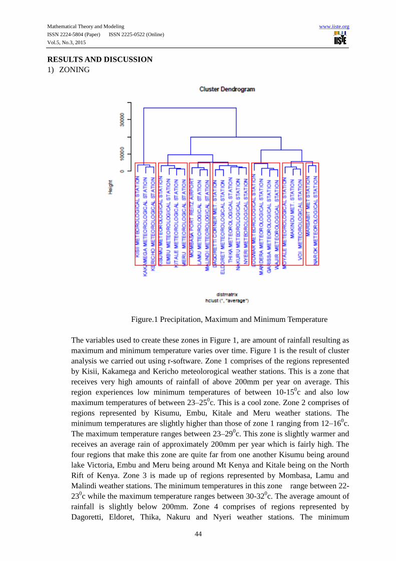
Figure.1 Precipitation, Maximum and Minimum Temperature

The variables used to create these zones in Figure 1, are amount of rainfall resulting as

maximum and minimum temperature varies over time. Figure 1 is the result of cluster

analysis we carried out using r-software. Zone 1 comprises of the regions represented

by Kisii, Kakamega and Kericho meteolorogical weather stations. This is a zone that

receives very high amounts of rainfall of above 200mm per year on average. This

region experiences low minimum temperatures of between 10-150c and also low

maximum temperatures of between 23–250c. This is a cool zone. Zone 2 comprises of

regions represented by Kisumu, Embu, Kitale and Meru weather stations. The

minimum temperatures are slightly higher than those of zone 1 ranging from 12–160c.

The maximum temperature ranges between 23–290c. This zone is slightly warmer and

receives an average rain of approximately 200mm per year which is fairly high. The

four regions that make this zone are quite far from one another Kisumu being around

lake Victoria, Embu and Meru being around Mt Kenya and Kitale being on the North

Rift of Kenya. Zone 3 is made up of regions represented by Mombasa, Lamu and

Malindi weather stations. The minimum temperatures in this zone range between 22-

230c while the maximum temperature ranges between 30-32

0c. The average amount of

rainfall is slightly below 200mm. Zone 4 comprises of regions represented by

Dagoretti, Eldoret, Thika, Nakuru and Nyeri weather stations. The minimum




Vol.5, No.3, 2015

45

temperature in this zone ranged between 9–120c while maximum temperature ranged

between 23–240c. The average amount of rain experienced in this zone is between 100

–150mm. The frequency of the rain in this zone is high. This makes the regions to be

wet. Zone 5 is made by regions represented by Lodwar, Mandera, Garissa and Wajir

weather stations whereby the minimum temperature ranged between 22–240c while

maximum temperature ranged between 32 -330c. The rainfall experienced in this

region was 30mm on average which is extremely low. This is a very hot and dry zone.

The regions of this zone are found on the northern part of Kenya. Zone 6 is made by

regions represented by Moyale, Makindu and Voi weather stations whose minimum

temperature ranged between 17 -190c while maximum temperature ranged between

27–290c. The rainfall experienced in this zone was between 50mm and 60mm which is

very low. This was a very hot and the second most dry zone. Geographically, Moyale

is in the northern Kenya while Makindu and Voi are on southern part of Kenya. Zone 7

comprised of regions represented by Marsabit and Narok weather stations, whose

minimum temperature ranged between 10 -160c while maximum temperature was

about 240c. The rainfall experienced in this zone was about 80mm which is fairly low.

This was a moderately warm and fairly dry zone. Marsabit lies in the northern Kenya

while Narok is in the southern part of Kenya.

We note here that the naming of the zone as number 1 to 7 in the figure 1 above, is

arbitrary and has no bearing to the amount of rainfall experienced by the zone.

2) GLMs

The data collected, was a count data. Several count models were investigated to see

which would best fit the data for each zone? The investigation was based on how well

Poisson, Quasi-Poisson and Negative Binomial Generalized Linear Models (GLMs)

would explain the relationship between rainfall, maximum temperature and minimum

temperature in all our zones above. Then the Akaike Information Criterion (AIC) was

used to select the best model that would help explain our problem. The best model is the

one that have the lowest AIC. In writing the glm model, x1 represented Maximum

temperature and x2 represented Minimum temperature while represented the mean

amount of rainfall.

The following are the results of models using the criterion of Precipitation, Maximum

And Minimum Temperature.




Vol.5, No.3, 2015

46

Zone 1; Precipitation, Maximum and Minimum temperature

Table 1; Kisii, Kakamega and Kericho




Vol.5, No.3, 2015

47

Zone 2;Precipitation, Maximum and Minimum temperature

Table 2; Kisumu, Embu, Meru and Kitale




Vol.5, No.3, 2015

48

Zone3; Precipitation, Maximum and Minimum temperature

Table 3; Mombasa, Lamu and Malindi




Vol.5, No.3, 2015

49


Table 4; Dagoretti, Eldoret, Thika, Nakuru and Nyeri




Vol.5, No.3, 2015

50

ZONE 5: Precipitation, Maximum and Minimum temperature

Table 5;Lodwar, Mandera, Garissa and Wajir




Vol.5, No.3, 2015

51

Zone 6; Precipitation, maximum and minimum temperature

Table 6; Moyale, Makindu and Voi




Vol.5, No.3, 2015

52


Table 7; Marsabit and Narok

Models

Table 1 represent the r-software output of the analysis for zone 1.The best model relating

precipitation, maximum and minimum temperature in zone 1 had an AIC of 12243. The

model was

21 113.01617.0699.7 xxIn 7

The mean amount of rainfall obtained as a result of maximum and minimum temperature was

21 113.01617.0699.7 xxe

The model (equation 7) showed that for every increase of c01 in maximum temperature, the

mean amount of rainfall decreased by 1.1755mm. At the same time an increase of 10c in

minimum temperature caused an increase in the amount of rainfall by an amount of

1.1196mm. The net effect was a decrease in the amount of rainfall with an amount of

0.1504mm.The dispersion parameter of 3.744 whose standard error is 0.163 shows that the

data from this zone was highly dispersed. The coefficients of the maximum and minimum

temperatures were by far less than 0.05. Hence these variables were significant in the




Vol.5, No.3, 2015

53

variability of rainfall.

In zone 2, the best model describing the relationship between Precipitation, maximum and

minimum temperature was extracted from table 2

21 017128.00544.00028.5 xxIn 8

With an AIC of 17162. The mean minimum amount of rainfall experienced in this zone

was

21 017128.00544.00028.5 XXe

For every 10c increase in maximum temperature, there was a decrease of the mean rainfall of

1.056 mm while an increase of 10c in minimum temperature caused an increase in rainfall of

1.0174mm. The overall effect was a decrease in the rainfall by 0.039mm. as deduced from

the model (equation 8). Data from this zone was overdispersed by a factor of 0.904 with

standard error of 0.0302. Low p-values for the data from this zone justify the significance of

the intercept 0 , coefficient 1 and 2 describing the variation of rainfall in this zone.

The best model to describe a good relationship between precipitation, maximum temperature

and minimum temperature in zone 3 was extracted from r-output table 3

21 126329.021704.009249.8 xxIn 9

While the mean amount of rainfall obtained due to the effect of maximum and minimum

temperature in this zone was 21 126329.0126329.009249.8 XXe

With an AIC of 30998. The dispersion parameter of data collected in this zone was 0.843 with

a standard error of 0.0203. In this zone, an increase of 10c in maximum temperature caused a

decrease of 1.2424mm of rainfall while it caused an increase of 1.13465mm of rainfall as

deduced from the model (equation 9). The net effect is a decrease in the amount of rainfall

experienced in this zone. The zone was becoming warm and drier.

From r-software output table 4, the best model to describe the relationship between

precipitation, maximum and minimum temperature in zone 4 was;

21 84096.043887.090442.0 xxIn 10

While the mean amount of rainfall in this zone was 1 20.90442 0.43887 0.84096x xe

With an AIC of 6533.6. Using the model (equation 10), An increase of 10c in maximum

and minimum temperature caused a 1.546mm decrease in the amount of rainfall and an

increase of 2.319mm of rainfall respectively. The net effect is an increase in the amount of

rainfall in this zone of about 0.773mm. The intercept and the coefficients of maximum and

minimum temperatures were very significant going by their very small p-value.

From the r-software output table5, the best model to describe the relationship between the

precipitation, maximum temperature and minimum temperature in zone 5 was

21 05144.013273.070110.6 xxIn 11

The mean amount of rainfall experienced in this zone due to combined effect of maximum




Vol.5, No.3, 2015

54

and minimum temperature was 21 05144.013273.070110.6 xxe

with an AIC of 10229. The

data dispersion from this zone was 0.6043 with a standard error of 0.0242. This model

(equation 11) indicates that a rise of 10c of maximum temperature, the rainfall decreased by

1.1419mm while for the same while for the same rise in minimum temperature causes an

increase of 1.05278mm. The net effect is a decrease in the amount of rainfall by 0.0891mm.

From the r-software output table 6, the best model to describe the relationship between the

precipitation, maximum temperature and minimum temperature in zone 6 was

1 213.7969 0.38025 0.9480In x x 12


and minimum temperature was 1 213.7969 0.38025 0.9480x xe with an AIC of 2384.8. The

data dispersion from this zone was 0.279 with a standard error of 0.06043. This model

(equation 12), indicates that a rise of 10c of maximum temperature, the rainfall decreased by

1.46265mm while for the same while for the same rise in minimum temperature causes an

increase of 2.5805mm. The net effect is an increase in the amount of rainfall by 1.1178mm.

Exploring the r-software output table 7, he best model to describe the relationship between

the precipitation, maximum temperature and minimum temperature in zone 7 was

1 22.60916 0.4179 0.63157In x x 13


and minimum temperature was 1 22.60916 0.4179 0.63157x xe with an AIC of 8236.9. The data

dispersion from this zone was 0.3145 with a standard error of 0.0133. This model (equation

13), indicates that a rise of 10c of maximum temperature, the rainfall decreased by 1.5188mm

while for the same while for the same rise in minimum temperature causes an increase of

1.0mm. The net effect is a decrease in the amount of rainfall by 0.0891mm.

An important point to note is that, different zones experience different amount of rainfall. This

is the amount of rainfall on average for the zone. Each zone is made up of one or more area(s)

and all the areas might not be receiving the same amount of rainfall, however the rain seasons

occur at the same time for all area(s) of the given zone

CONCLUSION AND RECOMMENDATION

In all the above zones, Negative binomial was the best model to describe the relationship

between the rainfall, maximum and minimum temperature. This is the model with the

lowest AIC value. The AIC criterion is used whenever there are some competing models

and the one with the lowest AIC is chosen. Using the GLMs, we were able to predict and

forecast the amount of rainfall expected in different zones. It was evident that for every rise of

10c the maximum amount of rainfall decreased, while the minimum amount of rainfall

increased. However, the amount of decrease was higher than the amount of increase in all

zones. The net effect is a decrease in rainfall experienced in all the zones except zone 6 where

the amount of increase of minimum rainfall was higher than the amount of decrease of

maximum rainfall.

Authorities should use negative binomial model to predict and forecast the amount of rainfall




Vol.5, No.3, 2015

55

expected in each zone using the temperature trends. Statisticians should do further research on

rainfall in zone 6.

References

Aldenderfer, M. a. (1985). Cluster Analysis. Sage Publication .

Aldenderfer, M. (1985). Cluster Analysis. Sage Publication .

Anderberg, M. (1973). Cluster Analysis for application. New Yolk: Academic Press.

Ball, G. a. (1967). A clustering technique for summarizing multivariate data. Behaviour

Science , 12:153-155.

Bazira, E. (1997). Predictability of East Africa seasonal rainfall using sea surface temperature.

Research Kenya.org .

Butterfield, R. (2009). Economic impacts of climate change (Kenya, Rwanda and Burundi.

ICPAC .

Cameron A.C, P. T. (1988). a macroeconomic model of the demand for health care and health

Insurance in Australia. Review of economic studies , 86-104.

Dolnicar, S. a. (2009). Challenging "Factor-Cluster segmentation". J Travel , Res47(1):63-71.

Everitt, B. L. (2001). Cluster Analysis. London: Arnold.

Gurmu, S. a. (1996). Excess zero in count models for recreational trips. journal of business

and economic statistics , 469-477.

Hilbe, J. (1994). Generalized Linear Models. London: Chapman and Hall.

Hoef, V. a. (2007). Quasi-Poissonvs Negative Binomial Regression:How should we model

overdispersed data. Washington: Ecological society of America.

Hoffman, J. (2004). Generalized Linear Models. New York: Springer Verlag.

Joeh, H. a. (2005). Generalized Poisson distribution:The property of mixture of Poisson and

Comparison with negative Binomial distribution. Biometrical journa , 219-229.

Kaufman, L. a. (2005). Finding groups in data. An introduction to cluster analysis. New Yolk:

Wiley Hoboken.

McCullagah, P. a. (1989). Generalized Linear Models. London: Chapman and Hall.




Vol.5, No.3, 2015

56

Nelder, J. a. (1972). Generalized Linear Models. journal of the royal statistical society ,

370-384.

Romesburg, C. (2004). Cluster analysis for reseachers. Manisvilles: Lulu press.

Sileshi, G. (2006). Selecting the right statistical model for analysis of insect count data by

using information theoretic measures. Bulletin of Entomological research , 479-458.

Toniazzo, T. D. (2008). Biasis and variability in the higam model. climate change research

group .

Tularam, G. a. (2010). Time series of rainfall and temperature interaction in coastal

catchments. Department of mathematics and Statistics .

Ward, J. J. (1963). hierarchical grouping to optimize an objective function. Journal of the

American Statistical Association , 58, 236-244.

Winkelmann, R. (1997). Duration Dependence and Dispersion in count data models. journal

of business and economic statistics , 467-474.

Youne's, M. a. (2012). Poisson Regression and zero inflated Poisson regression:Application to

private health Insurance data. European Actuarial journal , 8-14.


The IISTE is a pioneer in the Open-Access hosting service and academic event management.

The aim of the firm is Accelerating Global Knowledge Sharing.

More information about the firm can be found on the homepage:

http://www.iiste.org

CALL FOR JOURNAL PAPERS

There are more than 30 peer-reviewed academic journals hosted under the hosting platform.

Prospective authors of journals can find the submission instruction on the following

page: http://www.iiste.org/journals/ All the journals articles are available online to the

readers all over the world without financial, legal, or technical barriers other than those

inseparable from gaining access to the internet itself. Paper version of the journals is also

available upon request of readers and authors.

MORE RESOURCES

Book publication information: http://www.iiste.org/book/

Academic conference: http://www.iiste.org/conference/upcoming-conferences-call-for-paper/

IISTE Knowledge Sharing Partners

EBSCO, Index Copernicus, Ulrich's Periodicals Directory, JournalTOCS, PKP Open

Archives Harvester, Bielefeld Academic Search Engine, Elektronische Zeitschriftenbibliothek

EZB, Open J-Gate, OCLC WorldCat, Universe Digtial Library , NewJour, Google Scholar


http://www.iiste.org/journals/

http://www.iiste.org/book/

http://www.iiste.org/conference/upcoming-conferences-call-for-paper/

Generalized Linear Models for Rainfall Patterns In The ...

Documents

Transcript of Generalized Linear Models for Rainfall Patterns In The ...