Generalized latent variable models with non-linear effects
24
Copyright © The British Psychological Society Reproduction in any form (including the internet) is prohibited without prior permission from the Society Generalized latent variable models with non-linear effects Dimitris Rizopoulos 1 and Irini Moustaki 2,3 * 1 Erasmus University Medical Center, Rotterdam, The Netherlands 2 Athens University of Economics and Business, Athens, Greece 3 London School of Economics and Political Science, UK Until recently, item response models such as the factor analysis model for metric responses, the two-parameter logistic model for binary responses and the multinomial model for nominal responses considered only the main effects of latent variables without allowing for interaction or polynomial latent variable effects. However, non-linear relationships among the latent variables might be necessary in real applications. Methods for fitting models with non-linear latent terms have been developed mainly under the structural equation modelling approach. In this paper, we consider a latent variable model framework for mixed responses (metric and categorical) that allows inclusion of both non-linear latent and covariate effects. The model parameters are estimated using full maximum likelihood based on a hybrid integration–maximization algorithm. Finally, a method for obtaining factor scores based on multiple imputation is proposed here for the non-linear model. 1. Introduction The basic idea of latent variable analysis is to find, for a given set of response variables y 1 ;:::; y p , a set of latent variables or factors z 1 ;:::; z k , fewer in number than the observed variables, that contain essentially the same information about dependence. The factors are supposed to account for the dependencies among the response variables in the sense that if the factors were held fixed, the observed variables would be independent. In the literature, there are two main approaches to the analysis of multivariate data with latent variable models, namely the structural equation modelling (SEM) approach and the item response theory (IRT) approach. There are no differences between SEM and IRT when metric responses are analysed. In the case of categorical responses, the two approaches differ in the way they specify the probability of responding Prð y 1 ¼ * Correspondence should be addressed to Dimitris Rizopoulos, Department of Biostatistics, Erasmus University Medical Center, PO Box 2040, CA Rotterdam, The Netherlands (e-mail: [email protected]). The British Psychological Society 415 British Journal of Mathematical and Statistical Psychology (2008), 61, 415–438 q 2008 The British Psychological Society www.bpsjournals.co.uk DOI:10.1348/000711007X213963
-
Upload
dimitris-rizopoulos -
Category
Documents
-
view
212 -
download
0
Transcript of Generalized latent variable models with non-linear effects
Copyright © The British Psychological SocietyReproduction in any form (including the internet) is prohibited without prior permission from the Society
Generalized latent variable models withnon-linear effects
Dimitris Rizopoulos1 and Irini Moustaki2,3*1Erasmus University Medical Center, Rotterdam, The Netherlands2Athens University of Economics and Business, Athens, Greece3London School of Economics and Political Science, UK
Until recently, item response models such as the factor analysis model for metricresponses, the two-parameter logistic model for binary responses and the multinomialmodel for nominal responses considered only the main effects of latent variableswithout allowing for interaction or polynomial latent variable effects. However,non-linear relationships among the latent variables might be necessary in realapplications. Methods for fitting models with non-linear latent terms have beendeveloped mainly under the structural equation modelling approach. In this paper, weconsider a latent variable model framework for mixed responses (metric andcategorical) that allows inclusion of both non-linear latent and covariate effects. Themodel parameters are estimated using full maximum likelihood based on a hybridintegration–maximization algorithm. Finally, a method for obtaining factor scores basedon multiple imputation is proposed here for the non-linear model.
1. Introduction
The basic idea of latent variable analysis is to find, for a given set of response variables
y1; : : : ; yp, a set of latent variables or factors z1; : : : ; zk, fewer in number than
the observed variables, that contain essentially the same information about dependence.
The factors are supposed to account for the dependencies among the response variables in
the sense that if the factorswere held fixed, the observed variableswould be independent.
In the literature, there are two main approaches to the analysis of multivariate datawith latent variable models, namely the structural equation modelling (SEM) approach
and the item response theory (IRT) approach. There are no differences between SEM
and IRT when metric responses are analysed. In the case of categorical responses, the
two approaches differ in the way they specify the probability of responding Prð y1 ¼
* Correspondence should be addressed to Dimitris Rizopoulos, Department of Biostatistics, Erasmus University MedicalCenter, PO Box 2040, CA Rotterdam, The Netherlands (e-mail: [email protected]).
TheBritishPsychologicalSociety
415
British Journal of Mathematical and Statistical Psychology (2008), 61, 415–438
q 2008 The British Psychological Society
www.bpsjournals.co.uk
DOI:10.1348/000711007X213963
Copyright © The British Psychological SocietyReproduction in any form (including the internet) is prohibited without prior permission from the Society
a1; : : : ; yp ¼ apjz1; : : : ; zkÞ and the way they estimate the model, where a1; : : : ; ap
represent the different response categories of y1; : : : ; yp respectively.
Under the IRT approach, several authors such as Lawley and Maxwell (1971), Bock
(1972), Bock and Aitkin (1981) and Bartholomew and Knott (1999) have studied models
for binary, polytomous or metric variables. Recently, Bartholomew and Knott (1999),
Moustaki and Knott (2000) and Moustaki (2003) proposed a unified full informationmaximum likelihood (FIML) approach within the generalized linear model framework
(McCullagh & Nelder, 1989) that allows simultaneous analysis of all types of variables
(nominal, ordinal and metric) leading to a generalized latent variable model (GLVM). The
analysis of censored and uncensored variables is discussed in Moustaki and Steele
(2005). A similar framework is also discussed by Skrondal and Rabe-Hesketh (2004)
which includes multi-level random-effects models as a special case.
Under the SEM approach, ordinal and binary categorical variables are treated as
manifestations of underlying normal continuous variables. Different estimation methodshave been proposed (see Muthen, 1984; Lee, Poon, & Bentler, 1992; Joreskog, 1990,
1994; Shi & Lee 1998).
The GLVM that has been considered so far assumes additive latent and covariate
effects. However, inclusion of interactions and polynomial terms among latent variables
and covariates might be more appropriate in several settings. Applications of latent
variable models with non-linear terms in different disciplines such as marketing, social
psychology and political theory can be found in Schumacker and Marcoulides (1998)
and references therein. The idea of non-linear factor analysis goes back to Gibson (1960)and McDonald (1962, 1967a, 1967b, 1967c). McDonald (1962) discusses cases
where manifest variables are not monotonically related to latent variables. The
examples given are the typical middle item of an attitude scale and variables that
measure the intensity of attitude, which are known to have a U-shape relation to anxiety.
McDonald (1962, 1967a, 1967b, 1967c) has developed an estimation method for
fitting factor analysis models with polynomial expressions in the factors (quadratic
and interactions between the latent variables). In particular, McDonald (1962)
discussed the choice between a linear model with two factors and a model with asingle factor and quadratic functions of that single factor. In the linear two-factor
model the two factors are assumed to be independent, whereas in the non-linear
model the single factor and its quadratic form have correlation zero but are perfectly
curvilinearly related. Estimated individual ‘factor scores’ will give an indication of
whether a curvilinear relationship exists between the latent variables or whether two
distinct factors are needed. The ‘factor scores’ estimated are the known principal
components scores. His estimation method is based on determining through the
relationship between the ‘component scores’ the parameters defining the best-fitparabola. Estimates of the factor loadings of the non-linear model are obtained either
by rotation of the principal component loadings or by a least squares procedure.
McDonald (1967a, 1967b, 1967c) extended his non-linear model to allow for
interaction terms between the latent variables. Under the strong assumption that the
two latent variables are statistically independent, the three components z1, z2 and
z1 £ z2 are orthogonal. He considers three different models, a three-factor model
where the factors are statistically independent (model 1), a three-factor model with
orthogonal factors (model 2) and a model with two factors and the interaction termbetween them (model 3). The relationships between the factor loadings of models 1
and 2 and the factor loadings of models 2 and 3 are expressed through an orthogonal
transformation or through a least squares estimation. The suggested method provides
416 Dimitris Rizopoulos and Irini Moustaki

Copyright © The British Psychological SocietyReproduction in any form (including the internet) is prohibited without prior permission from the Society
information about whether a weaker model such as model 2 or a stronger model
such as model 1 or 3 is required to fit the data. Finally, Etezadi-Amoli and McDonald
(1983) proposed a maximum likelihood (ML) ratio and ordinary-least-squares methods
for estimating simultaneously factor loadings and factor scores for factor models with
both quadratic and interaction terms. In practice, their approach does not allow for a
simultaneous solution with respect to factor scores and loadings. They propose atwo-stage approach in which, for given values of the latent variables, the estimation
of the loadings and any other parameters is obtained by methods applied to
polynomial regression models. Etezadi-Amoli and McDonald (1983) have also shown
that the non-linear factor model eliminates rotational indeterminacy.
Bartlett (1953) pointed out that the inclusion of the interaction between two latent
variables in the linear factor analysis model will produce the same correlation properties
of the manifest variables as if a third genuine factor has been included. In addition,
Bartlett (1953), Etezadi-Amoli and McDonald (1983) and Bartholomew (1985) suggestedgraphical ways (bivariate plots of factor scores and components) of investigating the
necessity of non-linear terms.
Kenny and Judd (1984) also modelled latent variable interaction terms in one stage
under SEM. In their formulation, products of the observed variables are used as
indicators for the non-linear terms of the model. Their paper led to many
methodological papers discussing several aspects of non-linear latent variable
modelling, mainly under the SEM approach. In particular, Joreskog and Yang (1996)
and Yang (1997) studied the limitations of the Kenny–Judd model and found that oneproduct of observed variables is required to identify the model as long as intercept terms
and means are included. Problems that arise when using products of observed variables
are discussed in Arminger and Muthen (1998). These can be summarized in the difficulty
of computing covariance/correlation matrices among non-linear observed variables and
by the fact that the distribution of the endogenous latent variables that now includes
non-linear terms of exogenous latent variables is complex. This requires the setting of
non-linear constraints that complicate the specification of the model. From a practical
point of view, it is also true that different combinations of observed variables forconstructing the products might lead to different parameter estimates. Bollen (1995)
proposed a two-stage least squares method using instrumental variables. Also, Bollen
(1996) and Bollen and Paxton (1998) proposed a two-stage least squares method. Wall
and Amemiya (2000) proposed a method of moments and Wall and Amemiya (2001) an
appended product indicator procedure that produces consistent estimates, while Zhu
and Lee (1999) and Arminger and Muthen (1998) discussed a Bayesian estimation
method for models with metric data. Klein and Moosbrugger (2000) proposed a method
called the latent moderated structural equations approach that looks at conditionaldistributions of the metric observed variables that follow the normality assumption.
Variations of those methods as well as comparisons among them can be found in
Schumacker and Marcoulides (1998), Arminger and Muthen (1998), Moulder and Algina
(2002), Lee, Song, and Poon (2004) and references therein. Recently, a series of papers
by Lee and Zhu (2002), Lee and Song (2004a, 2004b), and Song and Lee (2004, 2006)
discuss Bayesian and ML estimation methods for non-linear factor models with mixed
data that allow for missing outcomes and hierarchical structures. The heavy integrations
involved in the Bayesian framework are overcome by the use of a data augmentationscheme and the use of the Gibbs sampler for sampling from complicated joint
distributions. In all those papers, dichotomous and ordinal variables are assumed to be
manifestations of underlying normally distributed continuous variables.
Generalized latent variable models 417
Copyright © The British Psychological SocietyReproduction in any form (including the internet) is prohibited without prior permission from the Society
In this paper, we incorporate non-linear terms in the factor model within the GLVM
framework presented by Bartholomew and Knott (1999). Bartholomew (1985) shifted
the interpretation of the factor analysis model from the unobserved factors to observed
statistics known as components that summarize the information conveyed in the
manifest variables. Those components for the q-factor model without non-linear terms
are q in number and are found to be a weighted sum of the manifest variables. Theweights are some function of the factor coefficients. Therefore, q components are a
sufficient summary for the manifest variables. In the same paper, Bartholomew stated
that in principle there is no problem over incorporating quadratic and interaction terms,
but he pointed out that although the inclusion of non-linear terms achieves a more
parsimonious model (reduced number of latent dimensions), the number of
components is not reduced. Bartholomew and McDonald (1986) pointed out that
only in the linear case does the number of latent variables equal the number of
components.The extended GLVM proposed here can easily incorporate non-linear terms without
making complex distributional assumptions for the joint distribution of the manifest
variables. In this paper, we consider only a measurement model with non-linear terms
where latent variables, covariates and their non-linear terms are taken to directly affect
the observed response variables. Categorical variables are naturally modelled as
members of the exponential family and are not treated as manifestations of underlying
normal continuous variables. However, we should note that the FIML method is, as
expected, computationally much more intensive than the limited-information methods.This is why we present the models with two latent variables, although the proposed
theoretical framework can be extended to handle non-linear terms with more, possibly
correlated, latent variables. Model parameters are estimated with the ML method using a
hybrid integration–maximization algorithm and standard errors are corrected for model
misspecification via the sandwich estimator. Finally, a multiple-imputation-like method
is proposed for computing factor scores under the proposed model.
2. Generalized latent variable models with non-linear terms
2.1. Model descriptionLet y1; : : : ; yp denote a set of manifest variables. We assume that the correlations among
the manifest variables y are explained by two latent variables z1 and z2, and some
observed covariates x. The distribution of each yi, given the two latent variables and the
covariates, is assumed to be a member of the exponential family, that is
pð yijz;x; ui;fiÞ ¼ expyiui 2 biðuiÞ
aiðfiÞþ dið yi;fiÞ
� �; i ¼ 1; : : : ; p; ð1Þ
where pð·Þ denotes a probability density function, and ui and fi are the natural and
dispersion parameters respectively. The subscript i in the functions bið·Þ, aið·Þ and dið·Þimplies that the distribution of each yi can be a different member of the exponential
family, for example binomial, Poisson, normal, gamma, thus allowing for mixed-type
response variables.As has been pointed out by many researchers, linear relationships between the latent
variables may not be adequate in many circumstances. Here we consider a more general
form of the GLVM which allows polynomial and interaction terms to be added in the
linear predictor. In general, we assume that the conditional means of the random
418 Dimitris Rizopoulos and Irini Moustaki

Copyright © The British Psychological SocietyReproduction in any form (including the internet) is prohibited without prior permission from the Society
component distributions are related to the systematic component generated by the
covariates and the latent variables through the formula
uiðmiðzÞÞ ¼ XbðxÞi þ ZbðzÞ
i ; ð2Þ
where uið·Þ and miðzÞ denote the link function and the conditional mean Eð yijzÞ foritem i respectively. The matrix X is a design matrix of the observed covariates associated
with an item-specific parameter vector bðxÞi and Z is a design matrix that is a function of
z1 and z2, including possibly non-linear terms, with an associated item-specific
parameter vector bðzÞi : Although inclusion of non-linear terms increases the complexity
of the linear predictor, their consideration might be necessary to describe more
complex relationships between the latent and observed variables.
The need to incorporate such terms in GLVM can arise in several settings. For
instance, in educational testing it is reasonable to assume that students’ abilities mayvary with socio-economic status or race. Justification regarding interactions between
latent variables follows in the same sense. Moreover, quadratic latent terms might be
useful when a non-linear relationship exists between the factors.
Our approach is advantageous from a numerical point of view for two main reasons.
First, theGLVM is based on conditional distributions ofobserved variables given the latent
variables and covariates that keep their form within the known distributions of the
exponential family. Second, for the two-factor model with non-linear terms the marginal
distribution of y is computed using a double integral instead of a higher-order integration,while allowing for more complex latent structures compared with a two-factor model.
2.2. Parameter estimation and standard errorsThe estimation of the model is based on ML, which is known to enjoy good optimalityproperties for large samples (Cox & Hinkley, 1974). Moreover, in latent variable
modelling, as also pointed out in Klein and Moosbrugger (2000), the option to use FIML
as opposed to limited-information approaches, typically used for interaction modelling,
gives important efficiency and power advantages. In general, for a random sample of size
n the log likelihood is written as
‘ðaÞ ¼Xnm¼1
log pð ym;aÞ ¼Xnm¼1
log
ð ðpðzmÞpð ymjzm;aÞdzm
� �; ð3Þ
where a is the vector of all the model parameters (factor loadings and scale parameters).
The latent variables zTm ¼ ðz1m; z2mÞ are assumed to follow a bivariate standard normal
distribution, with Corrðz1; z2Þ ¼ 0. For notational convenience, the condition on the
covariates is suppressed in the distributional expressions. Under the assumption of
conditional independence given the latent variables the manifest variables are taken to
be independent,
pð ymjzm;aÞ ¼Ypi¼1
pð yimjzm;aiÞ: ð4Þ
If the EM algorithm (Dempster, Laird, & Rubin, 1977) is to be used for estimating the
model parameters, one needs to write down the complete-data log likelihood given by
log pð y;z;aÞ ¼ log pð yjz;aÞ þ log pðzÞ: ð5Þ
Generalized latent variable models 419
Copyright © The British Psychological SocietyReproduction in any form (including the internet) is prohibited without prior permission from the Society
Taking into account (4) and (1), the maximization of the log likelihood is easy
since each pð yijzÞ is an ordinary generalized linear model (GLM) with linear predictor
given by (2).
A direct maximization of (3) can be achieved by solving the score equations
›‘ðaÞ=›a ¼ 0. In order to derive the score vector under (3), we introduce the following
notation: let W ¼ ðX ;Z) denote the full design matrix including both covariates
and latent variables, with an associated parameter vector bi ¼ ð½bðxÞi �T ; ½bðzÞ
i �T ÞT ; thus,wml denotes the mlth element of W and bil denotes the lth element of bi.The superscript T denotes the transpose. The first-order derivatives of (3) with respect
to bil take the form
›‘ðaÞ›bil
¼Xn0
m¼1
›
›bil
log
ð ðpðzmÞ·pð ymjzm;aÞdz1dz2
� �
¼Xn0
m¼1
ð ðpðzmÞpð ymjzm;aÞ
pð ym;aÞ›
›bil
yimuiðzmÞ2 biðuiðzmÞÞaiðfiÞ
þ dið yim;fiÞ� �
dz1dz2
¼Xn0
m¼1
ð ðpðzmjym;aÞ
aiðfiÞyim
›uiðzmÞ›bil
2›biðuiðzmÞÞ
›bil
� �dz1dz2
¼Xn0
m¼1
ð ð ½ yim 2 mimðzmÞ�wmlðzmÞVarð y ijzmÞu0
iðmimðzmÞÞpðzmjym;aÞdz1dz2;
ð6Þ
where u0ið�Þ denotes the first-order derivative of the link function. Moreover, note that
the summation is over the n0 # n individuals who contribute to the ith item, facilitating
the handling of non-balanced data sets.In connection with (5), it is also useful to observe that (6) represents both
the score vector of the observed-data log likelihood (3) and the expected value of the
score vector of the complete-data log likelihood (5) with respect to the posterior
distribution of the latent variables given the observed variables. This implies that (6) can
have a double role. In particular, if (6) is solved with respect to a (i.e. fixing pðzmjym;aÞto the values of a from the previous iteration), then this corresponds to an EM
algorithmwhereas if (6) is solved with respect to awithout assuming pðzmjym;aÞ fixed,then this corresponds to a maximization of the observed-data log likelihood. This in factallows an interplay between the EM and the maximization of the observed-data log
likelihood for the purpose of evaluating (6).
It is known that the ML estimator of the scale parameter fi is difficult to compute,
except from normal responses, thus leading to the use of alternative methods. For the
estimation of the scale parameter in GLVM, see Moustaki and Knott (2000).
Regarding the estimation of standard errors, it has been recognized (Busemeyer &
Jones, 1983; Ping, 2005) that the inclusion of non-linear terms could lead to potential
underestimation. Moreover, even though ML estimates are asymptotically efficient,latent variable modelling is prone to model misspecification since inference is based on
the marginal distribution of the manifest variables and the hypothesized latent structure
can only be checked implicitly. Misspecification is even more likely to occur when
non-linear terms are present, so a distinction between a third correlated factor and a
non-linear term is difficult to be made. Here, we propose a robust estimation for the
420 Dimitris Rizopoulos and Irini Moustaki
Copyright © The British Psychological SocietyReproduction in any form (including the internet) is prohibited without prior permission from the Society
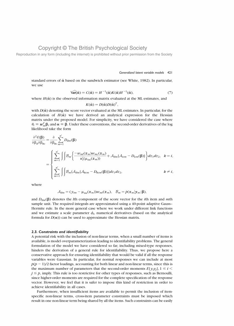
standard errors of a based on the sandwich estimator (see White, 1982). In particular,
we use
VcarðarðaÞ ¼ CðaÞ ¼ H 21ðaÞKðaÞH 21ðaÞ; ð7Þwhere HðaÞ is the observed information matrix evaluated at the ML estimates, and
KðaÞ ¼ DðaÞDðaÞT ;with DðaÞ denoting the score vector evaluated at the ML estimates. In particular, for thecalculation of HðaÞ we have derived an analytical expression for the Hessian
matrix under the proposed model. For simplicity, we have considered the case where
ui ; wTmbi and a ; b. Under these conventions, the second-order derivatives of the log
likelihood take the form
›2‘ðbÞ›bil›bkc
¼ ›
›bkc
Xn0
m¼1
DilmðbÞ
¼
Xn0
m¼1
ð ðBm
2wmlðzmÞwmcðzmÞu0iðmimðzmÞÞ
þAilm½Aicm 2DicmðbÞ�� �
dz1dz2; k ¼ i;
Xn0
m¼1
ð ðBm{Ailm½Akcm 2DkcmðbÞ�}dz1dz2; k– i;
8>>>>>>><>>>>>>>:where
Ailm ¼ ð yim 2mimðzmÞÞwmlðzmÞ; Bm ¼ pðzmjym;bÞ;
and DilmðbÞ denotes the lth component of the score vector for the ith item and mth
sample unit. The required integrals are approximated using a 40-point adaptive Gauss–
Hermite rule. In the more general case where we work under different link functionsand we estimate a scale parameter fi, numerical derivatives (based on the analytical
formula for DðaÞ) can be used to approximate the Hessian matrix.
2.3. Constraints and identifiabilityA potential risk with the inclusion of non-linear terms, when a small number of items is
available, is model overparameterization leading to identifiability problems. The general
formulation of the model we have considered so far, including mixed-type responses,hinders the derivation of a general rule for identifiability. Thus, we propose here a
conservative approach for ensuring identifiability that would be valid if all the response
variables were Gaussian. In particular, for normal responses we can include at most
pðp2 1Þ=2 factor loadings, accounting for both linear and non-linear terms, since this is
the maximum number of parameters that the second-order moments E½yiyj�; 1 # i ,
j # p; imply. This rule is too restrictive for other types of responses, such as Bernoulli,
since higher-order moments are required for the complete specification of the response
vector. However, we feel that it is safer to impose this kind of restriction in order toachieve identifiability in all cases.
Furthermore, when insufficient items are available to permit the inclusion of item-
specific non-linear terms, cross-item parameter constraints must be imposed which
result in one non-linear term being shared by all the items. Such constraints can be easily
Generalized latent variable models 421

Copyright © The British Psychological SocietyReproduction in any form (including the internet) is prohibited without prior permission from the Society
incorporated under the proposed model since only an extra summation, in the
expression for the score vector, is needed, that is,
›‘ðaÞ›bl
¼Xnm¼1
ð ðpðzmjym;aÞ
Xi[Pm
½yim 2 mimðzmÞ�wmlðzmÞVarð yijzmÞu0
iðmimðzmÞÞdz1dz2;
where bl now denotes the cross-item non-linear term and Pm is the set of items available
for the mth sample unit.
2.4. Extension to correlated latent variablesThe model considered so far assumes that two latent variables capture the associationsbetween the manifest variables. Two possible extensions within the GLVM framework
are to include more than two latent variables and to assume that these latent variables
are correlated. In particular, the model definition presented previously can be extended
to assume that Z contains n latent variables, where z ¼ ðz1; : : : ; znÞ follows a
multivariate normal distribution with mean zero and correlation matrix R. In this case, it
is easier to estimate R parameterized by c, using the EM algorithm. The parameter vector
a is now extended to include the parameter c of the correlation matrix R as well. The
derivatives with respect to c are
›‘ðaÞ›c
¼Xnm¼1
ð›
›clog pðzm;RðcÞÞ
� �pðzmjym;aÞdzm
¼ 1
2
Xnm¼1
trð2R21ðcÞK Þ þ trðHVmÞ þ €zTmH €zm;
where trð·Þ denotes the trace of a matrix, K ¼ ›RðcÞ=›c andH ¼ R21ðcÞKR21ðcÞ: Theelements of the matrix Vm are the conditional variances of the latent variables
zjmðVarðzjmjym;aÞÞ and the elements of the vector €zm are the conditional means
ðEðzjmjym;aÞÞ.Even though such an extension is mathematically possible, we feel that a model
including both non-linear and correlation terms between latent variables might be
difficult to estimate and interpret in real data applications, and usually a large number of
items and sample units will be required to obtain stable parameter estimates.
3. A hybrid integration–maximization algorithm
Due to the high-dimensional parameter space and the requirement for numerical
integration, the estimation of GLVM may be computationally demanding. Observe that
even in the simple setting, where all the conditional distributions pð yijzÞ, i ¼ 1; : : : ; p,and p(z) follow a normal distribution, the inclusion of non-linear terms does not result in
a marginal multivariate normal distribution, and therefore numerical integration cannotbe avoided. This has been recognized in the SEM approach by Joreskog and Yang (1996)
and discussed in more detail by Klein and Moosbrugger (2000).
A Gaussian quadrature rule is often used for approximating integrals by a finite
weighted sum of the integrand. In order to overcome approximation errors (see
Pinheiro & Bates, 1995; Lesaffre & Spiessens, 2001), the adaptive Gauss–Hermite rule is
422 Dimitris Rizopoulos and Irini Moustaki

Copyright © The British Psychological SocietyReproduction in any form (including the internet) is prohibited without prior permission from the Society
used here. In the adaptive quadrature rule, the integral is approximated according to the
expression (for simplicity we have dropped the sample unit subscript)ð ðf ðzÞdz1dz2 < det {�1=2}
XK1
k1¼1
XK2
k2¼1
hk1hk2 exp zTkzk� �
fffiffiffi2
p�1=2zk þ m
� �;
where f(z) denotes the integrand
pðzmÞpð ymjzm;aÞ
when the log likelihood (3) is computed, and
{ pðzmjym;aÞ½ yim 2 mimðzmÞ�wmlðzmÞ}{Varð yijzmÞu0iðmimðzmÞÞ}21
when the score vector (6) is computed, mz is the mode of f ðzÞ;�1=2 is the Cholesky
factor of
� ¼ 2›2 log f ðzÞ›z›zT
jz ¼ mz
� �21
;
and hk and zk ¼ ðz1k1 ; z2k2Þ are the weights and abscissae for the Gauss–Hermite rule.
We should also note that an adaptive quadrature rule also works in the case of correlatedlatent variables, in which case pðzm;RÞ should be used instead of pðzmÞ. Finally, underthe above transformation we obtain a function proportional to a Nð0; 221IÞ (I denotesthe identity matrix) density, which enhances accuracy since the Gauss–Hermite weight
function is proportional to this density.
An important drawback of the quadrature methods is that the number of integrand
evaluations required to approximate the integral increases exponentially with the
number of latent variables. To overcome this problem, a Monte Carlo integration
technique can be used as has been successfully applied in the SEM approach (Lee &Song, 2004a; Lee & Zhu, 2002). Monte Carlo integration is known to lead to good
integral approximations with fewer evaluations than the adaptive Gauss–Hermite
approach, especially in the case of many latent variables.
A common algorithm used to obtain the ML estimates in GLVMs is the EM algorithm, in
which the latent variables z are treated as missing data (Moustaki & Knott, 2000; Lee &
Song, 2004a). Although, EM is a stable algorithm leading to a likelihood increase at each
iteration, its convergence near the neighbourhood of the maximum can be very slow,
requiring many iterations. However, near the maximum, alternatives such as the Newton–Raphson and quasi-Newton Broyden–Fletcher–Goldfarb–Shanno (BFGS) algorithms
(Lange, 2004) provide faster convergence than the EM. Thus, we propose a hybrid
maximization approach, which starts with an EM algorithm for a moderate number of
iterations (e.g. 30), and then switches to the quasi-Newton BFGS algorithm, until
convergence. The required integrals are approximated by a 20-point adaptive Gauss–
Hermite rule. In this approach, the EM is mainly used as a refinement of the starting
estimates before beginning themainmaximization routine. The BFGSuses approximations
to theHessianbasedon the score vector and theparameter values, and thus avoids the extracalculations for computing theexactHessian.Using thishybridprocedure,weexpect that a
small number of BFGS iterationswill beneeded, since the EMquickly brings theparameters
near to the neighbourhood of the ML estimates. Furthermore, Monte Carlo EM or Markov
chain Monte Carlo is better suited to coping with the estimation of the high-dimensional
integrals involved as the number of factors increases.
Generalized latent variable models 423
Copyright © The British Psychological SocietyReproduction in any form (including the internet) is prohibited without prior permission from the Society
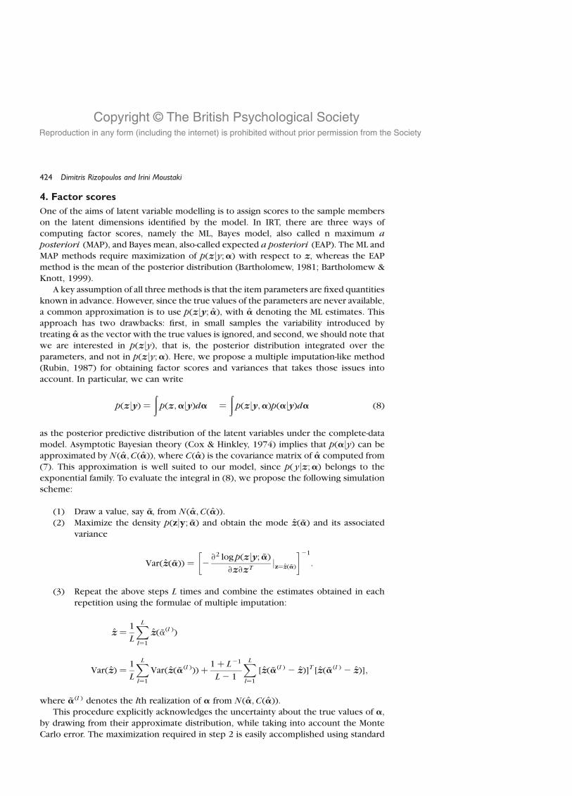
4. Factor scores
One of the aims of latent variable modelling is to assign scores to the sample members
on the latent dimensions identified by the model. In IRT, there are three ways ofcomputing factor scores, namely the ML, Bayes model, also called n maximum a
posteriori (MAP), and Bayes mean, also-called expected a posteriori (EAP). The ML and
MAP methods require maximization of pðzjy;aÞ with respect to z, whereas the EAP
method is the mean of the posterior distribution (Bartholomew, 1981; Bartholomew &
Knott, 1999).
A key assumption of all three methods is that the item parameters are fixed quantities
known in advance. However, since the true values of the parameters are never available,
a common approximation is to use pðzjy; aÞ; with a denoting the ML estimates. Thisapproach has two drawbacks: first, in small samples the variability introduced by
treating a as the vector with the true values is ignored, and second, we should note that
we are interested in pðzjyÞ, that is, the posterior distribution integrated over the
parameters, and not in pðzjy;aÞ. Here, we propose a multiple imputation-like method
(Rubin, 1987) for obtaining factor scores and variances that takes those issues into
account. In particular, we can write
pðzjyÞ ¼ðpðz;ajyÞda ¼
ðpðzjy;aÞpðajyÞda ð8Þ
as the posterior predictive distribution of the latent variables under the complete-data
model. Asymptotic Bayesian theory (Cox & Hinkley, 1974) implies that pðajyÞ can be
approximated by Nða;CðaÞÞ; where CðaÞ is the covariance matrix of a computed from
(7). This approximation is well suited to our model, since pð yjz;aÞ belongs to the
exponential family. To evaluate the integral in (8), we propose the following simulationscheme:
(1) Draw a value, say ~a, from Nða;CðaÞÞ:(2) Maximize the density pðzjy; ~aÞ and obtain the mode zð ~aÞ and its associated
variance
Varðzð ~aÞÞ ¼ 2›2 log pðzjy; ~aÞ
›z›zTjz¼zð ~aÞ
� �21
:
(3) Repeat the above steps L times and combine the estimates obtained in each
repetition using the formulae of multiple imputation:
z ¼ 1
L
XLl¼1
zð ~aðl ÞÞ
VarðzÞ ¼ 1
L
XLl¼1
Varðzð ~aðl ÞÞÞ þ 1þ L21
L2 1
XLl¼1
½zð ~aðl Þ 2 zÞ�T ½zð ~aðl Þ 2 zÞ�;
where ~aðl Þ denotes the lth realization of a from Nða;CðaÞÞ:This procedure explicitly acknowledges the uncertainty about the true values of a,
by drawing from their approximate distribution, while taking into account the Monte
Carlo error. The maximization required in step 2 is easily accomplished using standard
424 Dimitris Rizopoulos and Irini Moustaki

Copyright © The British Psychological SocietyReproduction in any form (including the internet) is prohibited without prior permission from the Society
numerical techniques, since as the number of items increases, pðzjy; ~aÞ converges to a
concave function with respect to z with a single maximum.
In cases where more information (e.g. specific quantiles, shape) about the posterior
distribution is needed, we could easily modify step 2 of the above scheme and instead of
maximizing draw a value from this density. In particular, either a Metropolis or a
rejection sampling step (e.g. Booth & Hobert, 1999) could be adopted to get a sample ofL values from
pðzjy; ~aðl ÞÞ/ pð yjz; ~aðl ÞÞpðzÞ/ expXpi¼1
yi ~uðl Þi 2 bið ~u
ðl Þi Þ
aið ~fðl Þi Þ
" #2
zTz
2
( ):
These values can then be used to extract any required information about this distribution.
The choice of L depends on the quantities wewish to estimate aswell as the assumptionsabout pðzjyÞ we are willing to make. For instance, if we can assume approximate
normality of pðzjyÞ (which will be the case for large p), then we need only enough
repetitions to reliably estimate the first twomoments, inwhich case L ¼ 20 or 30 suffices.
If we do not wish to restrict to the normality assumption and, moreover, want to estimate
extreme quantiles (e.g. calculate 95% considence intervals), then L-values of the order of
500 will be required. Finally, it is straightforward to extend the proposed method for
obtaining factor scores to handle correlated latent variables by considering pðzm;RÞ inthe place of pðzmÞ.
5. Simulation
A simulation study is performed to numerically evaluate the performance of the proposed
model. In particular, two non-linear models are considered: One that contains two latent
variables and their interaction, and one that contains one latent variable and its quadratic
effect. For each non-linear model, data are generated under four scenarios: (i) 10 items
and 500 sample units, (ii) 10 items and 1,000 sample units, (iii) 30 items and 500 sampleunits, and (iv) 30 items and 1,000 sample units. We denote by bi0 the intercept,
with bi1;bi2 the loadings for the first and second factor respectively, and with bi3
the loadings of the non-linear term (i ¼ 1; : : : ; p). The parameter values used are as
follows: b0 ¼ seqð22:5; 2:5; pÞ, b1 ¼ seqð22; 2; pÞ, b2 ¼ seqð2;22; pÞ, and
b3 ¼ seqð21:5; 1:5; pÞ, where p denotes the number of items in the corresponding
scenario and seq(a, b, p) denotes a regular sequence from a to b of length p
(e.g. seqð22; 2; 5Þ ¼ 22;21; 0; 1; 2). Under each scenario, 1,000 data sets are
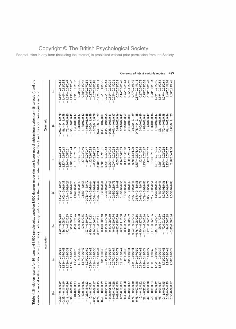
simulated, assuming dichotomous manifest variables and standard normally distributedlatent variables. Tables 1–4 present the bias and root mean square error for each
parameter.
We can see that bias is relatively small in all cases and does not seem to be significant
in any of them. Bias decreases as sample size and the number of items increase.
Moreover, the model with the interaction term shows greater bias than the model with
the quadratic effect. This could probably be attributed to the higher complexity of the
model with the interaction term.
6. Application
As an illustration of the proposed modelling framework, here we discuss an example
taken from a section of the 1990 Workplace Industrial Relations Survey (WIRS) dealing
Generalized latent variable models 425

Copyright © The British Psychological SocietyReproduction in any form (including the internet) is prohibited without prior permission from the Society
Table
1.S
imula
tion
resu
lts
for
10
item
san
d500
sam
ple
units,
bas
edon
1,0
00
dat
ase
tsunder
the
two-f
acto
rm
odel
with
anin
tera
ctio
nte
rm(inte
ract
ion),
and
the
one-
fact
or
model
with
aquad
ratic
term
(quad
ratic)
.Eac
hen
trya/b/c
conta
ins
the
true
par
amet
erva
luea,
the
bia
sb
and
the
root
mea
nsq
uar
eer
rorc
Inte
ract
ion
Quad
ratic
bi0
bi1
bi2
bi3
bi0
bi1
bi3
22.5
0/2
0.7
6/4
.34
22.0
0/2
0.4
3/2
.29
2.0
0/2
0.2
2/1
.92
21.5
0/2
0.1
0/0
.84
22.5
0/2
0.4
4/1
.56
22.0
0/2
0.3
3/1
.29
21.5
0/2
0.2
3/0
.97
21.9
4/2
0.0
4/1
.92
21.5
6/0
.04/0
.70
1.5
6/0
.09/0
.85
21.1
7/0
.21/1
.45
21.9
4/2
0.0
7/0
.64
21.5
6/0
.01/0
.69
21.1
7/2
0.0
1/0
.73
21.3
9/0
.35/1
.75
21.1
1/0
.60/4
.44
1.1
1/2
0.6
8/3
.94
20.8
3/2
0.3
7/2
.35
21.3
9/0
.04/0
.69
21.1
1/0
.24/0
.98
20.8
3/0
.38/1
.44
20.8
3/2
0.2
4/1
.90
20.6
7/2
0.1
1/0
.93
0.6
7/2
0.0
0/3
.45
20.5
0/0
.03/1
.13
20.8
3/0
.44/1
.62
20.6
7/2
0.3
3/2
.64
20.5
0/2
0.1
4/2
.16
20.2
8/0
.10/1
.03
20.2
2/0
.27/1
.59
0.2
2/0
.36/1
.77
20.1
7/0
.63/4
.21
20.2
8/2
0.0
7/1
.67
20.2
2/2
0.1
1/1
.05
20.1
7/2
0.0
5/0
.61
0.2
8/0
.62/3
.92
0.2
2/0
.39/2
.20
20.2
2/0
.18/1
.96
0.1
7/0
.11/1
.13
0.2
8/0
.04/0
.69
0.2
2/0
.10/1
.10
0.1
7/0
.07/1
.71
0.8
3/0
.04/3
.51
0.6
7/2
0.0
3/1
.24
20.6
7/2
0.0
5/1
.02
0.5
0/2
0.1
8/1
.50
0.8
3/0
.34/2
.56
0.6
7/0
.20/2
.70
0.5
0/2
0.0
2/2
.43
1.3
9/2
0.3
4/1
.65
1.1
1/2
0.5
5/4
.01
21.1
1/2
0.2
2/2
.88
0.8
3/0
.08/2
.56
1.3
9/0
.05/2
.02
1.1
1/0
.02/1
.66
0.8
3/2
0.0
1/1
.15
1.9
4/0
.02/1
.92
1.5
6/2
0.0
5/1
.10
21.5
6/2
0.0
2/2
.59
1.1
7/0
.02/1
.03
1.9
4/2
0.0
2/0
.91
1.5
6/0
.02/0
.98
1.1
7/0
.04/1
.22
2.5
0/0
.03/1
.04
2.0
0/0
.05/1
.64
22.0
0/0
.05/2
.12
1.5
0/0
.04/2
.99
2.5
0/2
0.0
5/1
.68
2.0
0/0
.14/2
.39
1.5
0/0
.11/2
.40
426 Dimitris Rizopoulos and Irini Moustaki

Copyright © The British Psychological SocietyReproduction in any form (including the internet) is prohibited without prior permission from the Society
Table
2.Si
mula
tion
resu
lts
for
10
item
san
d1,0
00
sam
ple
units,
bas
edon
1,0
00
dat
ase
tsunder
the
two-f
acto
rm
odel
with
anin
tera
ctio
nte
rm(inte
ract
ion),
and
the
one-
fact
or
model
with
aquad
ratic
term
(quad
ratic)
.Eac
hen
trya/b/c
conta
ins
the
true
par
amet
erva
luea,
the
bia
sb
and
the
root
mea
nsq
uar
eer
rorc
Inte
ract
ion
Quad
ratic
bi0
bi1
bi0
bi1
bi0
bi1
bi0
22.5
0/2
0.3
8/2
.05
22.0
0/2
0.2
6/1
.21
2.0
0/2
0.1
4/1
.00
21.5
0/2
0.0
8/0
.64
22.5
0/2
0.3
5/1
.30
22.0
0/2
0.2
4/0
.96
21.5
0/2
0.1
7/0
.65
21.9
4/2
0.0
3/0
.41
21.5
6/0
.02/0
.35
1.5
6/0
.07/0
.89
21.1
7/0
.16/1
.27
21.9
4/2
0.0
5/0
.58
21.5
6/0
.01/0
.51
21.1
7/2
0.0
0/0
.51
21.3
9/0
.27/1
.32
21.1
1/0
.40/2
.31
1.1
1/2
0.3
3/2
.16
20.8
3/2
0.1
9/1
.29
21.3
9/0
.05/0
.54
21.1
1/0
.17/0
.79
20.8
3/0
.23/1
.02
20.8
3/2
0.1
1/1
.06
20.6
7/2
0.0
6/0
.81
0.6
7/2
0.0
3/0
.80
20.5
0/2
0.0
0/0
.73
20.8
3/0
.38/1
.31
20.6
7/2
0.0
4/2
.19
20.5
0/0
.02/1
.65
20.2
8/0
.06/1
.07
20.2
2/0
.14/1
.31
0.2
2/0
.20/1
.22
20.1
7/0
.42/2
.30
20.2
8/2
0.0
4/1
.04
20.2
2/2
0.0
5/0
.70
20.1
7/2
0.0
2/0
.54
0.2
8/0
.44/1
.85
0.2
2/0
.26/1
.26
20.2
2/0
.13/1
.14
0.1
7/0
.05/0
.82
0.2
8/0
.03/0
.54
0.2
2/0
.04/0
.72
0.1
7/0
.04/1
.30
0.8
3/0
.01/0
.82
0.6
7/2
0.0
2/0
.69
20.6
7/2
0.0
5/1
.15
0.5
0/2
0.1
5/1
.42
0.8
3/0
.06/1
.77
0.6
7/0
.25/2
.28
0.5
0/0
.09/2
.07
1.3
9/2
0.2
4/1
.49
1.1
1/2
0.3
8/2
.12
21.1
1/2
0.1
1/2
.09
0.8
3/0
.04/1
.36
1.3
9/0
.11/1
.61
1.1
1/0
.07/1
.06
0.8
3/0
.02/0
.82
1.9
4/2
0.0
1/1
.19
1.5
6/2
0.0
3/0
.80
21.5
6/2
0.0
2/0
.61
1.1
7/0
.03/0
.55
1.9
4/2
0.0
2/0
.60
1.5
6/0
.01/0
.59
1.1
7/0
.01/0
.84
2.5
0/0
.00/1
.22
2.0
0/0
.01/1
.38
22.0
0/0
.02/1
.35
1.5
0/0
.11/2
.13
2.5
0/2
0.0
5/1
.30
2.0
0/2
0.0
4/1
.71
1.5
0/0
.03/2
.11
Generalized latent variable models 427

Copyright © The British Psychological SocietyReproduction in any form (including the internet) is prohibited without prior permission from the Society
Table
3.S
imula
tion
resu
lts
for
30
item
san
d500
sam
ple
units,
bas
edon
1,0
00
dat
ase
tsunder
the
two-f
acto
rm
odel
with
anin
tera
ctio
nte
rm(inte
ract
ion),
and
the
one-
fact
or
model
with
aquad
ratic
term
(quad
ratic)
.Eac
hen
trya/b/c
conta
ins
the
true
par
amet
erva
luea,
the
bia
sb
and
the
root
mea
nsq
uar
eer
rorc
Inte
ract
ion
Quad
ratic
bi0
bi1
bi0
bi1
bi0
bi1
bi0
22.5
0/2
0.2
9/0
.78
22.0
0/2
0.2
8/0
.76
2.0
0/2
0.2
2/0
.81
21.5
0/2
0.1
9/0
.66
22.5
0/2
0.2
3/1
.11
22.0
0/2
0.2
3/1
.03
21.5
0/2
0.1
5/0
.89
22.3
3/2
0.1
8/0
.63
21.8
6/2
0.1
4/0
.55
1.8
6/2
0.1
1/0
.54
21.4
0/2
0.1
0/0
.47
22.3
3/2
0.2
3/0
.82
21.8
6/2
0.1
4/0
.74
21.4
0/2
0.1
0/0
.65
22.1
6/2
0.0
8/0
.43
21.7
2/2
0.0
6/0
.39
1.7
2/2
0.0
5/0
.36
21.2
9/2
0.0
4/0
.32
22.1
6/2
0.1
0/0
.61
21.7
2/2
0.0
8/0
.57
21.2
9/2
0.0
5/0
.50
21.9
8/2
0.0
2/0
.31
21.5
9/2
0.0
2/0
.29
1.5
9/2
0.0
0/0
.27
21.1
9/0
.01/0
.28
21.9
8/2
0.0
3/0
.49
21.5
9/2
0.0
2/0
.46
21.1
9/2
0.0
1/0
.45
21.8
1/0
.01/0
.29
21.4
5/0
.02/0
.31
1.4
5/0
.03/0
.32
21.0
9/0
.05/0
.38
21.8
1/0
.00/0
.43
21.4
5/0
.01/0
.41
21.0
9/2
0.0
0/0
.40
21.6
4/0
.06/0
.39
21.3
1/0
.08/0
.46
1.3
1/0
.10/0
.47
20.9
8/0
.12/0
.54
21.6
4/2
0.0
0/0
.41
21.3
1/2
0.0
1/0
.43
20.9
8/0
.01/0
.43
21.4
7/0
.16/0
.55
21.1
7/0
.15/0
.59
1.1
7/0
.20/0
.64
20.8
8/0
.26/0
.71
21.4
7/0
.00/0
.46
21.1
7/0
.03/0
.46
20.8
8/0
.04/0
.48
21.2
9/0
.23/0
.73
21.0
3/0
.33/0
.82
1.0
3/2
0.3
6/0
.87
20.7
8/2
0.3
1/0
.86
21.2
9/0
.07/0
.51
21.0
3/0
.09/0
.52
20.7
8/0
.08/0
.58
21.1
2/2
0.2
6/0
.85
20.9
0/2
0.2
2/0
.76
0.9
0/2
0.2
0/0
.76
20.6
7/2
0.1
4/0
.66
21.1
2/0
.10/0
.65
20.9
0/0
.13/0
.75
20.6
7/0
.20/0
.88
20.9
5/2
0.1
4/0
.67
20.7
6/2
0.0
8/0
.62
0.7
6/2
0.1
2/0
.59
20.5
7/2
0.0
9/0
.53
20.9
5/0
.17/0
.97
20.7
6/0
.22/1
.15
20.5
7/0
.25/1
.15
20.7
8/2
0.0
5/0
.52
20.6
2/2
0.0
3/0
.48
0.6
2/2
0.0
3/0
.47
20.4
7/2
0.0
2/0
.45
20.7
8/2
0.5
2/1
.99
20.6
2/2
0.2
4/1
.83
20.4
7/2
0.1
3/1
.57
20.6
0/0
.01/0
.44
20.4
8/0
.01/0
.44
0.4
8/0
.02/0
.45
20.3
6/0
.02/0
.46
20.6
0/2
0.0
7/1
.35
20.4
8/2
0.1
5/1
.23
20.3
6/2
0.1
2/0
.99
20.4
3/0
.02/0
.48
20.3
4/0
.06/0
.53
0.3
4/0
.07/0
.56
20.2
6/0
.08/0
.59
20.4
3/2
0.0
6/0
.83
20.3
4/2
0.1
1/0
.75
20.2
6/2
0.0
6/0
.57
20.2
6/0
.08/0
.61
20.2
1/0
.12/0
.66
0.2
1/0
.17/0
.69
20.1
6/0
.18/0
.72
20.2
6/2
0.0
2/0
.52
20.2
1/2
0.0
5/0
.47
20.1
6/2
0.0
1/0
.45
20.0
9/0
.21/0
.74
20.0
7/0
.27/0
.82
0.0
7/0
.28/0
.85
20.0
5/0
.32/0
.91
20.0
9/2
0.0
1/0
.44
20.0
7/2
0.0
1/0
.41
20.0
5/2
0.0
0/0
.40
0.0
9/0
.36/0
.87
0.0
7/0
.31/0
.87
20.0
7/0
.30/0
.93
0.0
5/0
.27/0
.77
0.0
9/0
.01/0
.42
0.0
7/0
.02/0
.43
0.0
5/0
.03/0
.44
0.2
6/0
.23/0
.75
0.2
1/0
.19/0
.69
20.2
1/0
.14/0
.68
0.1
6/0
.13/0
.63
0.2
6/0
.04/0
.45
0.2
1/0
.05/0
.50
0.1
6/0
.04/0
.51
0.4
3/0
.08/0
.58
0.3
4/0
.06/0
.53
20.3
4/0
.06/0
.52
0.2
6/0
.03/0
.48
0.4
3/0
.05/0
.60
0.3
4/0
.05/0
.67
0.2
6/0
.07/0
.80
0.6
0/0
.03/0
.46
0.4
8/0
.01/0
.45
20.4
8/0
.01/0
.44
0.3
6/2
0.0
1/0
.44
0.6
0/0
.13/1
.03
0.4
8/0
.12/1
.24
0.3
6/0
.23/1
.50
0.7
8/2
0.0
2/0
.44
0.6
2/2
0.0
4/0
.47
20.6
2/2
0.0
5/0
.49
0.4
7/2
0.0
6/0
.53
0.7
8/0
.25/1
.72
0.6
2/0
.23/1
.95
0.4
7/0
.61/2
.03
0.9
5/2
0.0
8/0
.55
0.7
6/2
0.1
2/0
.64
20.7
6/2
0.1
5/0
.61
0.5
7/2
0.1
4/0
.67
0.9
5/2
0.4
7/1
.93
0.7
6/2
0.3
2/1
.79
0.5
7/2
0.1
5/1
.59
1.1
2/2
0.1
8/0
.70
0.9
0/2
0.2
1/0
.73
20.9
0/2
0.2
4/0
.75
0.6
7/2
0.3
5/0
.82
1.1
2/0
.05/1
.35
0.9
0/2
0.0
7/1
.26
0.6
7/2
0.0
2/1
.03
1.2
9/2
0.3
1/0
.82
1.0
3/2
0.3
8/0
.91
21.0
3/2
0.1
1/0
.99
0.7
8/2
0.0
2/0
.94
1.2
9/0
.00/0
.88
1.0
3/2
0.0
1/0
.79
0.7
8/2
0.0
0/0
.65
1.4
7/2
0.0
6/1
.02
1.1
7/2
0.0
0/0
.86
21.1
7/2
0.0
4/0
.84
0.8
8/2
0.0
4/0
.79
1.4
7/2
0.0
0/0
.59
1.1
7/0
.01/0
.54
0.8
8/2
0.0
1/0
.50
1.6
4/2
0.0
1/0
.76
1.3
1/2
0.0
3/0
.70
21.3
1/0
.03/0
.64
0.9
8/2
0.0
1/0
.59
1.6
4/2
0.0
0/0
.46
1.3
1/2
0.0
1/0
.41
0.9
8/2
0.0
1/0
.39
1.8
1/2
0.0
3/0
.57
1.4
5/2
0.0
3/0
.52
21.4
5/2
0.0
1/0
.47
1.0
9/2
0.0
0/0
.46
1.8
1/2
0.0
1/0
.40
1.4
5/0
.01/0
.44
1.0
9/0
.01/0
.45
1.9
8/2
0.0
0/0
.45
1.5
9/0
.00/0
.44
21.5
9/0
.01/0
.45
1.1
9/2
0.0
1/0
.48
1.9
8/0
.00/0
.51
1.5
9/0
.00/0
.54
1.1
9/0
.01/0
.58
2.1
6/0
.04/0
.52
1.7
2/0
.03/0
.59
21.7
2/0
.03/0
.61
1.2
9/2
0.0
0/0
.66
2.1
6/2
0.0
1/0
.66
1.7
2/2
0.0
1/0
.73
1.2
9/0
.04/0
.88
2.3
3/0
.02/0
.70
1.8
6/0
.06/0
.75
21.8
6/0
.03/0
.77
1.4
0/0
.01/0
.82
2.3
3/0
.08/1
.11
1.8
6/0
.05/1
.26
1.4
0/0
.08/1
.54
2.5
0/2
0.0
2/0
.86
2.0
0/0
.01/0
.90
22.0
0/0
.03/0
.94
1.5
0/0
.13/0
.98
2.5
0/0
.21/1
.73
2.0
0/0
.22/1
.87
1.5
0/0
.39/1
.98
428 Dimitris Rizopoulos and Irini Moustaki
Copyright © The British Psychological SocietyReproduction in any form (including the internet) is prohibited without prior permission from the Society
Table
4.S
imula
tion
resu
lts
for
30
item
san
d1,0
00
sam
ple
units,
bas
edon
1,0
00
dat
aset
sunder
the
two-f
acto
rm
odel
with
anin
tera
ctio
nte
rm(inte
ract
ion),
and
the
one-
fact
or
model
with
aquad
ratic
term
(quad
ratic)
.Eac
hen
trya/b/c
conta
ins
the
true
par
amet
erva
luea,
the
bia
sb
and
the
root
mea
nsq
uar
eer
rorc
Inte
ract
ion
Quad
ratic
bi0
bi1
bi0
bi1
bi0
bi1
bi0
22.5
0/2
0.1
8/0
.69
22.0
0/2
0.1
6/0
.58
2.0
0/2
0.1
5/0
.58
21.5
0/2
0.1
5/0
.54
22.5
0/2
0.2
2/0
.84
22.0
0/2
0.1
5/0
.78
21.5
0/2
0.1
7/0
.68
22.3
3/2
0.1
1/0
.49
21.8
6/2
0.0
9/0
.48
1.8
6/2
0.0
8/0
.41
21.4
0/2
0.0
6/0
.39
22.3
3/2
0.1
4/0
.63
21.8
6/2
0.1
1/0
.58
21.4
0/2
0.1
2/0
.55
22.1
6/2
0.0
5/0
.34
21.7
2/2
0.0
4/0
.31
1.7
2/2
0.0
3/0
.29
21.2
9/2
0.0
2/0
.27
22.1
6/2
0.0
8/0
.51
21.7
2/2
0.0
7/0
.49
21.2
9/2
0.0
4/0
.47
21.9
8/2
0.0
2/0
.25
21.5
9/2
0.0
1/0
.24
1.5
9/0
.00/0
.23
21.1
9/0
.01/0
.23
21.9
8/2
0.0
3/0
.44
21.5
9/2
0.0
3/0
.42
21.1
9/2
0.0
2/0
.40
21.8
1/0
.01/0
.23
21.4
5/0
.02/0
.25
1.4
5/0
.02/0
.26
21.0
9/0
.03/0
.29
21.8
1/2
0.0
2/0
.39
21.4
5/0
.00/0
.37
21.0
9/2
0.0
1/0
.36
21.6
4/0
.03/0
.31
21.3
1/0
.05/0
.35
1.3
1/0
.06/0
.38
20.9
8/0
.08/0
.43
21.6
4/0
.01/0
.36
21.3
1/0
.01/0
.37
20.9
8/0
.01/0
.38
21.4
7/0
.10/0
.46
21.1
7/0
.10/0
.49
1.1
7/0
.13/0
.55
20.8
8/0
.16/0
.58
21.4
7/0
.03/0
.40
21.1
7/0
.02/0
.42
20.8
8/0
.04/0
.44
21.2
9/0
.19/0
.63
21.0
3/0
.20/0
.62
1.0
3/2
0.1
9/0
.79
20.7
8/2
0.1
9/0
.72
21.2
9/0
.04/0
.47
21.0
3/0
.08/0
.48
20.7
8/0
.07/0
.51
21.1
2/2
0.1
7/0
.71
20.9
0/2
0.1
2/0
.65
0.9
0/2
0.1
1/0
.63
20.6
7/2
0.0
9/0
.64
21.1
2/0
.10/0
.58
20.9
0/0
.11/0
.59
20.6
7/0
.13/0
.64
20.9
5/2
0.0
6/0
.57
20.7
6/2
0.0
7/0
.55
0.7
6/2
0.0
4/0
.51
20.5
7/2
0.0
1/0
.48
20.9
5/0
.14/0
.69
20.7
6/0
.19/0
.78
20.5
7/0
.20/0
.85
20.7
8/2
0.0
1/0
.45
20.6
2/2
0.0
2/0
.44
0.6
2/2
0.0
2/0
.41
20.4
7/2
0.0
1/0
.42
20.7
8/2
0.2
2/1
.42
20.6
2/2
0.1
8/1
.27
20.4
7/2
0.1
0/1
.11
20.6
0/2
0.0
1/0
.39
20.4
8/0
.00/0
.40
0.4
8/0
.00/0
.40
20.3
6/0
.02/0
.41
20.6
0/2
0.0
9/0
.91
20.4
8/2
0.0
7/0
.81
20.3
6/2
0.1
0/0
.70
20.4
3/0
.04/0
.44
20.3
4/0
.04/0
.46
0.3
4/0
.03/0
.48
20.2
6/0
.03/0
.50
20.4
3/2
0.0
6/0
.63
20.3
4/2
0.0
5/0
.55
20.2
6/2
0.0
4/0
.51
20.2
6/0
.06/0
.55
20.2
1/0
.06/0
.57
0.2
1/0
.08/0
.60
20.1
6/0
.11/0
.63
20.2
6/2
0.0
4/0
.45
20.2
1/2
0.0
3/0
.41
20.1
6/2
0.0
3/0
.39
20.0
9/0
.12/0
.68
20.0
7/0
.16/0
.69
0.0
7/0
.20/0
.74
20.0
5/0
.23/0
.75
20.0
9/2
0.0
2/0
.38
20.0
7/2
0.0
1/0
.37
20.0
5/2
0.0
1/0
.36
0.0
9/0
.25/0
.79
0.0
7/0
.17/0
.71
20.0
7/0
.19/0
.70
0.0
5/0
.16/0
.68
0.0
9/0
.02/0
.36
0.0
7/0
.02/0
.36
0.0
5/0
.02/0
.38
0.2
6/0
.12/0
.63
0.2
1/0
.10/0
.62
20.2
1/0
.11/0
.58
0.1
6/0
.09/0
.55
0.2
6/0
.04/0
.39
0.2
1/0
.04/0
.42
0.1
6/0
.06/0
.45
0.4
3/0
.04/0
.50
0.3
4/0
.05/0
.48
20.3
4/0
.05/0
.46
0.2
6/0
.03/0
.44
0.4
3/0
.04/0
.48
0.3
4/0
.05/0
.52
0.2
6/0
.06/0
.61
0.6
0/0
.01/0
.42
0.4
8/0
.01/0
.41
20.4
8/2
0.0
0/0
.39
0.3
6/2
0.0
1/0
.40
0.6
0/0
.09/0
.73
0.4
8/0
.08/0
.81
0.3
6/0
.11/0
.97
0.7
8/2
0.0
1/0
.40
0.6
2/2
0.0
1/0
.41
20.6
2/2
0.0
3/0
.43
0.4
7/2
0.0
6/0
.46
0.7
8/0
.13/1
.08
0.6
2/0
.19/1
.29
0.4
7/0
.22/1
.45
0.9
5/2
0.0
7/0
.48
0.7
6/2
0.0
7/0
.52
20.7
6/2
0.0
8/0
.56
0.5
7/2
0.1
3/0
.59
0.9
5/2
0.1
3/1
.42
0.7
6/2
0.1
0/1
.28
0.5
7/2
0.0
1/1
.16
1.1
2/2
0.1
3/0
.62
0.9
0/2
0.0
9/0
.63
20.9
0/2
0.1
7/0
.66
0.6
7/2
0.1
9/0
.71
1.1
2/0
.01/0
.96
0.9
0/0
.02/0
.89
0.6
7/0
.04/0
.75
1.2
9/2
0.2
2/0
.73
1.0
3/2
0.1
8/0
.74
21.0
3/2
0.0
4/0
.86
0.7
8/2
0.0
6/0
.82
1.2
9/2
0.0
2/0
.67
1.0
3/0
.02/0
.61
0.7
8/0
.03/0
.56
1.4
7/2
0.0
7/0
.78
1.1
7/2
0.0
2/0
.77
21.1
7/2
0.0
6/0
.72
0.8
8/2
0.0
6/0
.71
1.4
7/0
.02/0
.52
1.1
7/0
.02/0
.47
0.8
8/0
.00/0
.43
1.6
4/2
0.0
4/0
.64
1.3
1/2
0.0
2/0
.60
21.3
1/2
0.0
6/0
.56
0.9
8/2
0.0
3/0
.51
1.6
4/0
.02/0
.41
1.3
1/0
.00/0
.36
0.9
8/0
.00/0
.34
1.8
1/2
0.0
3/0
.49
1.4
5/2
0.0
2/0
.44
21.4
5/2
0.0
2/0
.41
1.0
9/0
.01/0
.39
1.8
1/2
0.0
1/0
.35
1.4
5/0
.00/0
.37
1.0
9/2
0.0
1/0
.40
1.9
8/2
0.0
1/0
.37
1.5
9/2
0.0
0/0
.38
21.5
9/0
.01/0
.39
1.1
9/0
.02/0
.41
1.9
8/2
0.0
1/0
.43
1.5
9/2
0.0
1/0
.48
1.1
9/2
0.0
2/0
.51
2.1
6/0
.03/0
.45
1.7
2/0
.02/0
.48
21.7
2/0
.02/0
.52
1.2
9/0
.08/0
.56
2.1
6/2
0.0
2/0
.56
1.7
2/2
0.0
3/0
.58
1.2
9/2
0.0
2/0
.64
2.3
3/0
.04/0
.59
1.8
6/0
.06/0
.66
21.8
6/0
.04/0
.68
1.4
0/0
.06/0
.70
2.3
3/2
0.0
3/0
.77
1.8
6/2
0.0
3/0
.86
1.4
0/0
.01/1
.01
2.5
0/0
.06/0
.77
2.0
0/0
.07/0
.79
22.0
0/0
.00/0
.84
1.5
0/0
.07/0
.83
2.5
0/0
.06/1
.08
2.0
0/0
.11/1
.29
1.5
0/0
.23/1
.48
Generalized latent variable models 429

Copyright © The British Psychological SocietyReproduction in any form (including the internet) is prohibited without prior permission from the Society
with management–worker consultation in firms, see http://www.niesr.ac.uk/research/
WERS98/. A subset of these data is used here that consists of 1,005 firms and concerns
non-manual workers. Previous analyses of these data can be found in Bartholomew
(1998) and in Bartholomew, Steele, Moustaki, and Galbraith (2008). The questions asked
are given below.
Please consider the most recent change involving the introduction of the new plant,
machinery and equipment. Were discussions or consultations of any of the type on this card
held either about the introduction of the change or about the way it was to be
implemented?
(1) Informal discussion with individual workers.(2) Meeting with groups of workers.(3) Discussions in established joint consultative committee.(4) Discussions in specially constituted committee to consider the change.(5) Discussions with the union representatives at the establishment.(6) Discussions with paid union officials from outside.
All the six items measure the amount of consultation that takes place in firms at
different levels of the firm structure and cover a range of informal to formal types
of consultation. Those firms that place a high value on consultation might be expectedto use all or most consultation practices. We should mention that the above items were
not initially constructed to form a scale and therefore our analysis is completely
exploratory.
All items are binary and no covariate information is available. Therefore, we use the
GLVM in the case of binary responses that depends only on the latent design matrix Z.Assuming that each manifest variable yi has a Bernoulli distribution with expected value
piðzÞ and using the logit link function: we get
uiðzÞ ¼ logitðpiðzÞÞ ¼ bi0 þ Zbzi ;
where
piðzÞ ¼ Prð yi ¼ 1jzÞ ¼ exp ðuiðzÞÞ1þ exp ðuiðzÞÞ
:
The previous analysis of the WIRS data revealed that neither the one- nor two-factor
model provides a good fit to the data. In particular, the two-factor model improved the fit
on the two-way margins but not on the three-way margins (see Bartholomew, 1998;
Bartholomew et al., 2008).The use of two latent variables seems logical for the WIRS data, since the items
potentially identify two styles of consultation, namely formal and informal. We
extend the simple two-factor model to allow for an interaction between the two
latent variables. However, as stated in Section 2.3, the inclusion of item-specific non-
linear terms is not advisable here due to the small number of items. Thus, a model
with one cross-item interaction term is fitted. In order to ensure convergence, the
model was fitted under a variety of starting values for the majority of which the same
solution was obtained with the highest log-likelihood value. The likelihood ratio teststatistic between the two-factor and the interaction model equals 93.13, which is
highly significant at one degree of freedom. However, the use of a likelihood ratio test
for the goodness of fit of the model is not advisable here since many expected
frequencies are smaller than 5 and thus the approximation of the distribution of the
statistic by a x2 distribution may not be appropriate. Thus, the fit in the two- and
430 Dimitris Rizopoulos and Irini Moustaki
Copyright © The British Psychological SocietyReproduction in any form (including the internet) is prohibited without prior permission from the Society
three-way margins is checked instead. We found that all the two- and three-way
residuals have acceptable values, which is less than 1 and 2.18 respectively
(according to Bartholomew et al., 2008, values greater than 3 or 4 are indicative of
poor fit). The good fit of the model is also apparent from a direct inspection of the
fitted frequencies given in Table 6.
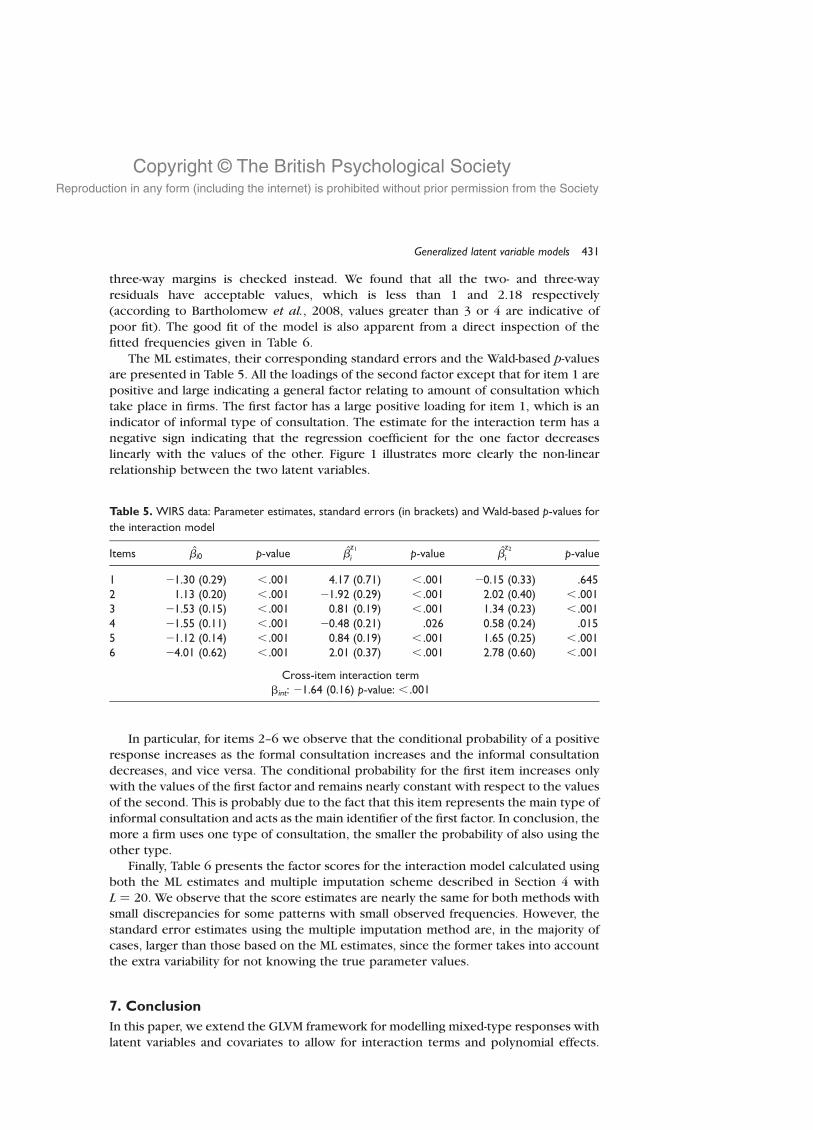
The ML estimates, their corresponding standard errors and the Wald-based p-valuesare presented in Table 5. All the loadings of the second factor except that for item 1 are
positive and large indicating a general factor relating to amount of consultation which
take place in firms. The first factor has a large positive loading for item 1, which is an
indicator of informal type of consultation. The estimate for the interaction term has a
negative sign indicating that the regression coefficient for the one factor decreases
linearly with the values of the other. Figure 1 illustrates more clearly the non-linear
relationship between the two latent variables.
In particular, for items 2–6 we observe that the conditional probability of a positiveresponse increases as the formal consultation increases and the informal consultation
decreases, and vice versa. The conditional probability for the first item increases only
with the values of the first factor and remains nearly constant with respect to the values
of the second. This is probably due to the fact that this item represents the main type of
informal consultation and acts as the main identifier of the first factor. In conclusion, the
more a firm uses one type of consultation, the smaller the probability of also using the
other type.
Finally, Table 6 presents the factor scores for the interaction model calculated usingboth the ML estimates and multiple imputation scheme described in Section 4 with
L ¼ 20. We observe that the score estimates are nearly the same for both methods with
small discrepancies for some patterns with small observed frequencies. However, the
standard error estimates using the multiple imputation method are, in the majority of
cases, larger than those based on the ML estimates, since the former takes into account
the extra variability for not knowing the true parameter values.
7. Conclusion
In this paper, we extend the GLVM framework for modelling mixed-type responses with
latent variables and covariates to allow for interaction terms and polynomial effects.
Table 5. WIRS data: Parameter estimates, standard errors (in brackets) and Wald-based p-values for
the interaction model
Items bi0 p-value bz1
i p-value bz2
i p-value
1 21.30 (0.29) , .001 4.17 (0.71) , .001 20.15 (0.33) .6452 1.13 (0.20) , .001 21.92 (0.29) , .001 2.02 (0.40) , .0013 21.53 (0.15) , .001 0.81 (0.19) , .001 1.34 (0.23) , .0014 21.55 (0.11) , .001 20.48 (0.21) .026 0.58 (0.24) .0155 21.12 (0.14) , .001 0.84 (0.19) , .001 1.65 (0.25) , .0016 24.01 (0.62) , .001 2.01 (0.37) , .001 2.78 (0.60) , .001
Cross-item interaction termbint: 21.64 (0.16) p-value: , .001
Generalized latent variable models 431
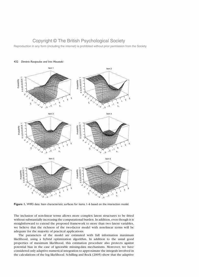
Copyright © The British Psychological SocietyReproduction in any form (including the internet) is prohibited without prior permission from the Society
The inclusion of non-linear terms allows more complex latent structures to be fitted
without substantially increasing the computational burden. In addition, even though it is
straightforward to extend the proposed framework to more than two latent variables,
we believe that the richness of the two-factor model with non-linear terms will be
adequate for the majority of practical applications.The parameters of the model are estimated with full information maximum
likelihood, using a hybrid optimization algorithm. In addition to the usual good
properties of maximum likelihood, this estimation procedure also protects against
potential bias in the case of ignorable missing-data mechanisms. Moreover, we have
considered only adaptive numerical integration to approximate the integrals involved in
the calculations of the log likelihood. Schilling and Bock (2005) show that the adaptive
Figure 1. WIRS data: Item characteristic surfaces for items 1–6 based on the interaction model.
432 Dimitris Rizopoulos and Irini Moustaki
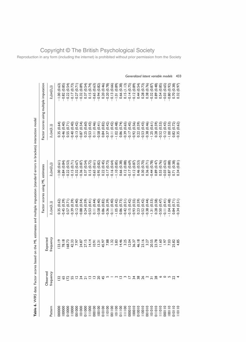
Copyright © The British Psychological SocietyReproduction in any form (including the internet) is prohibited without prior permission from the Society
Table
6.
WIR
Sdat
a:Fa
ctor
score
sbas
edon
the
ML
estim
ates
and
multip
leim
puta
tion
(sta
ndar
der
rors
inbra
cket
s)in
tera
ctio
nm
odel
Obse
rved
freq
uen
cyExpec
ted
freq
uen
cy
Fact
or
score
susi
ng
ML
estim
ates
Fact
or
score
susi
ng
multip
leim
puta
tion
Pat
tern
z 1ðse
ðz1ÞÞ
z 2ðse
ðz2ÞÞ
z 1ðse
ðz1ÞÞ
z 2ðse
ðz2ÞÞ
000000
132
133.1
90.3
5(0
.62)
21.0
0(0
.61)
0.3
5(0
.64)
21.0
0(0
.63)
100000
65
78.1
82
0.4
5(0
.39)
20.8
4(0
.84)
20.4
6(0
.40)
20.8
2(0
.85)
010000
172
168.7
30.5
7(0
.71)
20.2
2(0
.53)
0.5
5(0
.71)
20.2
2(0
.54)
110000
55
42.3
32
0.3
9(0
.39)
20.1
5(0
.71)
20.4
0(0
.40)
20.1
7(0
.73)
001000
12
7.9
72
0.1
2(0
.40)
20.3
2(0
.67)
20.1
3(0
.42)
20.2
7(0
.71)
101000
24
24.8
72
0.8
8(0
.54)
20.3
6(0
.87)
20.8
7(0
.54)
20.3
2(0
.89)
011000
21
27.1
50.2
4(0
.59)
0.3
7(0
.54)
0.2
5(0
.60)
0.3
7(0
.54)
111000
13
14.1
42
0.5
3(0
.41)
0.1
5(0
.72)
20.5
3(0
.43)
0.1
5(0
.74)
000100
13
10.9
10.1
1(0
.44)
20.6
5(0
.61)
0.1
1(0
.46)
20.6
5(0
.63)
100100
20
13.3
12
0.5
8(0
.40)
20.9
5(0
.82)
20.5
8(0
.41)
20.9
4(0
.82)
010100
45
45.9
70.8
6(0
.82)
0.2
2(0
.45)
0.8
4(0
.82)
0.2
0(0
.46)
110100
57.8
82
0.3
6(0
.39)
20.1
7(0
.73)
20.3
7(0
.42)
20.2
0(0
.78)
001100
11.3
22
0.1
1(0
.40)
20.1
6(0
.64)
20.1
1(0
.42)
20.1
3(0
.66)
101100
25.8
32
1.0
5(0
.42)
21.1
0(0
.85)
21.0
2(0
.48)
21.0
1(0
.89)
011100
13
14.4
60.8
6(0
.73)
0.6
6(0
.38)
0.8
6(0
.74)
0.6
6(0
.38)
111100
33.2
52
0.4
2(0
.51)
0.1
2(0
.88)
20.3
9(0
.65)
0.1
5(1
.13)
000010
17
12.0
42
0.1
5(0
.42)
20.1
7(0
.69)
20.1
7(0
.45)
20.1
4(0
.75)
100010
34
36.3
72
0.9
3(0
.55)
20.1
2(0
.87)
20.9
2(0
.56)
20.1
2(0
.89)
010010
38
46.1
80.2
3(0
.59)
0.4
6(0
.53)
0.2
2(0
.59)
0.4
4(0
.54)
110010
26
23.1
62
0.5
2(0
.42)
0.3
0(0
.70)
20.5
3(0
.43)
0.2
8(0
.73)
001010
23.2
72
0.3
8(0
.44)
0.3
6(0
.71)
20.3
8(0
.46)
0.3
8(0
.76)
101010
31
20.5
52
1.3
1(0
.53)
20.4
4(0
.78)
21.2
5(0
.61)
20.3
2(0
.87)
011010
28
23.7
80.2
8(0
.58)
0.8
9(0
.47)
0.2
8(0
.59)
0.8
9(0
.48)
111010
611.6
02
0.5
0(0
.47)
0.5
5(0
.76)
20.5
2(0
.53)
0.5
4(0
.85)
000110
01.9
72
0.1
1(0
.41)
20.0
3(0
.63)
20.1
2(0
.43)
20.0
3(0
.65)
100110
57.0
32
1.0
4(0
.48)
20.8
7(0
.88)
21.0
0(0
.53)
20.8
0(0
.92)
010110
22
25.8
20.8
4(0
.71)
0.7
1(0
.38)
0.8
2(0
.72)
0.7
0(0
.38)
110110
44.8
52
0.3
4(0
.51)
0.3
4(0
.81)
20.3
5(0
.62)
0.3
2(0
.97)
Generalized latent variable models 433
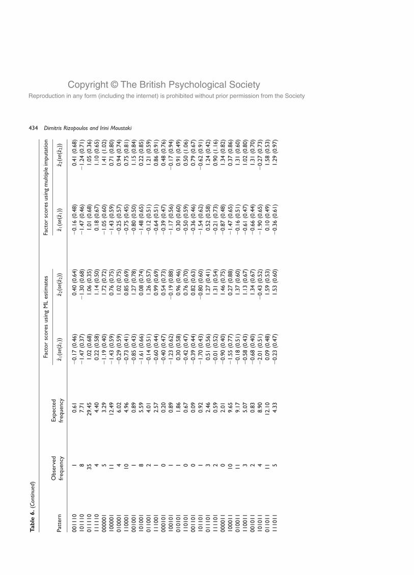
Copyright © The British Psychological SocietyReproduction in any form (including the internet) is prohibited without prior permission from the Society
Table
6.
(Continued)
Obse
rved
freq
uen
cyExpec
ted
freq
uen
cy
Fact
or
score
susi
ng
ML
estim
ates
Fact
or
score
susi
ng
multip
leim
puta
tion
Pat
tern
z 1ðse
ðz1ÞÞ
z 2ðse
ðz2ÞÞ
z 1ðse
ðz1ÞÞ
z 2ðse
ðz2ÞÞ
001110
10.6
12
0.1
7(0
.46)
0.4
0(0
.64)
20.1
6(0
.48)
0.4
1(0
.68)
101110
87.7
12
1.4
7(0
.37)
21.3
0(0
.68)
21.4
7(0
.46)
21.2
4(0
.71)
011110
35
29.4
51.0
2(0
.68)
1.0
6(0
.35)
1.0
1(0
.68)
1.0
5(0
.36)
111110
44.4
00.2
2(0
.58)
1.1
4(0
.50)
0.1
8(0
.67)
1.1
0(0
.65)
000001
53.2
92
1.1
9(0
.40)
1.7
2(0
.72)
21.0
5(0
.60)
1.4
1(1
.02)
100001
11
12.4
92
1.4
3(0
.59)
0.7
6(0
.75)
21.4
3(0
.59)
0.7
1(0
.80)
010001
46.0
22
0.2
9(0
.59)
1.0
2(0
.75)
20.2
5(0
.57)
0.9
4(0
.74)
110001
10
4.9
62
0.7
3(0
.41)
0.8
5(0
.69)
20.7
5(0
.45)
0.7
5(0
.81)
001001
10.8
92
0.8
5(0
.43)
1.2
7(0
.78)
20.8
0(0
.50)
1.1
5(0
.84)
101001
85.5
92
1.6
1(0
.66)
0.0
8(0
.74)
21.4
8(0
.65)
0.2
2(0
.85)
011001
24.0
12
0.1
4(0
.51)
1.2
6(0
.57)
20.1
2(0
.51)
1.2
1(0
.59)
111001
12.5
72
0.6
0(0
.44)
0.9
9(0
.69)
20.6
4(0
.51)
0.8
6(0
.91)
000101
00.2
02
0.4
0(0
.47)
0.5
4(0
.73)
20.3
9(0
.47)
0.4
8(0
.76)
100101
10.8
92
1.2
3(0
.62)
20.1
9(0
.88)
21.1
7(0
.56)
20.1
7(0
.94)
010101
11.8
60.3
0(0
.58)
0.9
6(0
.46)
0.3
0(0
.60)
0.9
1(0
.49)
110101
00.6
72
0.4
2(0
.47)
0.7
6(0
.70)
20.5
0(0
.59)
0.5
0(1
.06)
001101
00.0
92
0.3
9(0
.44)
0.8
2(0
.63)
20.3
6(0
.46)
0.7
9(0
.67)
101101
10.9
22
1.7
0(0
.43)
20.8
0(0
.60)
21.5
4(0
.62)
20.6
2(0
.91)
011101
32.4
60.5
1(0
.56)
1.2
7(0
.41)
0.5
2(0
.58)
1.2
4(0
.42)
111101
20.5
92
0.0
1(0
.52)
1.3
1(0
.54)
20.2
1(0
.73)
0.9
0(1
.16)
000011
02.0
12
0.9
0(0
.40)
1.4
6(0
.75)
20.8
7(0
.48)
1.3
4(0
.82)
100011
10
9.6
52
1.5
5(0
.77)
0.2
7(0
.88)
21.4
7(0
.65)
0.3
7(0
.86)
010011
11
9.1
72
0.1
8(0
.51)
1.3
7(0
.60)
20.1
6(0
.51)
1.3
1(0
.60)
110011
35.0
72
0.5
8(0
.43)
1.1
3(0
.67)
20.6
1(0
.47)
1.0
2(0
.80)
001011
20.8
32
0.6
8(0
.40)
1.3
4(0
.67)
20.6
6(0
.44)
1.3
1(0
.70)
101011
48.9
02
2.0
1(0
.51)
20.4
3(0
.52)
21.9
0(0
.65)
20.2
7(0
.73)
011011
11
12.1
00.0
9(0
.48)
1.5
9(0
.53)
0.1
0(0
.49)
1.5
8(0
.53)
111011
54.3
32
0.2
3(0
.47)
1.5
3(0
.60)
20.3
6(0
.61)
1.2
9(0
.97)
434 Dimitris Rizopoulos and Irini Moustaki
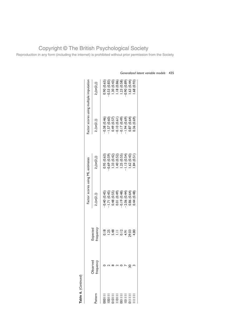
Copyright © The British Psychological SocietyReproduction in any form (including the internet) is prohibited without prior permission from the Society
Table
6.
(Continued)
Obse
rved
freq
uen
cyExpec
ted
freq
uen
cy
Fact
or
score
susi
ng
ML
estim
ates
Fact
or
score
susi
ng
multip
leim
puta
tion
Pat
tern
z 1ðse
ðz1ÞÞ
z 2ðse
ðz2ÞÞ
z 1ðse
ðz1ÞÞ
z 2ðse
ðz2ÞÞ
000111
00.1
82
0.4
0(0
.45)
0.9
5(0
.63)
20.3
8(0
.46)
0.9
0(0
.65)
100111
21.2
52
1.7
1(0
.45)
20.6
9(0
.59)
21.5
7(0
.60)
20.5
3(0
.83)
010111
85.4
80.4
8(0
.55)
1.3
3(0
.42)
0.4
9(0
.57)
1.3
0(0
.43)
110111
21.1
10.0
1(0
.49)
1.4
0(0
.52)
20.1
0(0
.61)
1.1
8(0
.86)
001111
00.1
22
0.1
9(0
.48)
1.2
5(0
.55)
20.1
7(0
.49)
1.2
3(0
.58)
101111
74.9
12
2.0
6(0
.44)
21.1
3(0
.54)
21.9
4(0
.69)
20.9
0(0
.89)
011111
30
29.0
30.8
6(0
.64)
1.6
2(0
.43)
0.8
7(0
.64)
1.6
3(0
.44)
111111
34.8
00.4
4(0
.48)
1.8
4(0
.51)
0.3
6(0
.69)
1.6
8(0
.93)
Generalized latent variable models 435
Copyright © The British Psychological SocietyReproduction in any form (including the internet) is prohibited without prior permission from the Society
approximation can produce fast and accurate solutions using even only two points on
each dimension. Alternatively, Laplace approximations (see Huber, Ronchetti, &
Victoria-Feser, 2004) and Monte Carlo methods can be used. These approximations are
expected to work better as the number of items increases, since the integrand tends to
be proportional to a Gaussian. We should note that Laplace approximations succeed for
continuous as well as count and binomial data. However, a small number ofdichotomous items can lead to a severe integration error.
Furthermore, a method to obtain factor scores is proposed that explicitly
approximates the modes of the integrated posterior distribution pðzjyÞ taking into
account the variability of the ML estimates This method will be particularly useful for
small sample sizes since the variability around the ML estimates would be greater.
However, these attractive features are achieved at the expense of L extra optimizations.
Finally, some forms of the proposed GLV model can be fitted using the freet available
ltm package (Rizopoulos, 2006) for R available from http://cran.r-project.org/.
References
Arminger, G., & Muthen, B. (1998). A Bayesian approach to nonlinear latent variables models using
the Gibbs sampler and the Metropolis–Hastings algorithm. Psychometrika, 63, 271–300.
Bartholomew, D. J. (1981). Posterior analysis of the factor model. British Journal of Mathematical
and Statistical Psychology, 34, 93–99.
Bartholomew, D. J. (1985). Foundations of factor analysis: Some practical implications. British
Journal of Mathematical and Statistical Psychology, 38, 1–10.
Bartholomew, D. J. (1998). Scaling unobservable constructs in social science. Applied Statistics,
47, 1–13.
Bartholomew, D. J., & Knott, M. (1999). Latent variable models and factor analysis (2nd ed.).
London: Arnold.
Bartholomew, D. J., & McDonald, R. P. (1986). The foundations of factor analysis: A further
comment. British Journal of Mathematical and Statistical Psychology, 39, 228–229.
Bartholomew, D. J., Steele, F., Moustaki, I., & Galbraith, J. (2008). Analysis of multivariate social
science data. Boca Raton, FL: Chapman & Hall/CRC.
Bartlett, M. S. (1953). Factor analysis in psychology as a statistician sees it. Uppsala Symposium
Psychological Factor Analysis (pp. 23–34). Nordisk Psykologi’s Monograph Series No.3.
Copenhagen: Ejnav Mundsgaards Stockholm: Almqvist & Wiksell.
Bock, R. (1972). Estimating item parameters and latent ability when responses are scored in two or
more nominal categories. Psychometrika, 37, 29–51.
Bock, R., & Aitkin, M. (1981). Marginal maximum likelihood estimation of item parameters:
Application of an EM algorithm. Psychometrika, 46, 443–459.
Bollen, K. (1995). Structural equation models that are nonlinear in latent variables: A least-squares
estimator. Sociological Methodology, 25, 223–251.
Bollen, K. (1996). An alternative two stage least squares (2SLS) estimator for latent variable
equation. Psychometrika, 61, 109–121.
Bollen, K., & Paxton, P. (1998). Two-stage least squares estimation of interaction effects. In
R. Schumacker & G. Marcoulides (Eds.), Interaction and nonlinear effects in structural
equation models (pp. 125–151). Mahwah, NJ: Erlbaum.
Booth, J., & Hobert, J. (1999). Maximizing generalized linear mixed model likelihoods with an
automated Monte Carlo EM algorithm. Journal of the Royal Statistical Society, Series B, 61,
265–285.
Busemeyer, J., & Jones, L. (1983). Analysis of multiplicative combination rules when the causal
variables are measured with error. Psychological Bulletin, 93, 549–562.
Cox, D., & Hinkley, D. (1974). Theoretical statistics. London: Chapman & Hall.
436 Dimitris Rizopoulos and Irini Moustaki
Copyright © The British Psychological SocietyReproduction in any form (including the internet) is prohibited without prior permission from the Society
Dempster, A., Laird, N., & Rubin, D. (1977). Maximum likelihood from incomplete data via the EM
algorithm. Journal of the Royal Statistical Society, Series B, 39, 1–38.
Etezadi-Amoli, J., & McDonald, R. P. (1983). A second generation nonlinear factor analysis.
Psychometrika, 48, 315–342.
Gibson, W. (1960). Nonlinear factors in two dimensions. Psychometrika, 25, 381–392.
Huber, P., Ronchetti, E., & Victoria-Feser, M. (2004). Estimation of generalized latent trait models.
Journal of the Royal Statistical Society, Series B, 66, 893–908.
Joreskog, K. (1990). New developments in LISREL: Analysis of ordinal variables using polychoric
correlations and weighted least squares. Quality and Quantity, 24, 387–404.
Joreskog, K. (1994). On the estimation of polychoric correlations and their asymptotic covariance
matrix. Psychometrika, 59, 381–389.
Joreskog, K., & Yang, F. (1996). Nonlinear structural equation models: The Kenny–Judd model
with interaction effects. In G. Marcoulides & R. Schumacker (Eds.), Advanced structural
equation modeling (pp. 57–88). Mahwah, NJ: Erlbaum.
Kenny, D., & Judd, C. (1984). Estimating the nonlinear and interactive effects of latent variables.
Psychological Bulletin, 96, 201–210.
Klein, A., & Moosbrugger, H. (2000). Maximum likelihood estimation of latent interaction effects
with the LMS method. Psychometrika, 65, 457–474.
Lange, K. (2004). Optimization. New York: Springer-Verlag.
Lawley, D., & Maxwell, A. (1971). Factor analysis as a statistical method (2nd ed.). London:
Butterworth.
Lee, S.-Y., Poon, W.-Y., & Bentler, P. (1992). Structural equation models with continuous and
polytomous variables. Psychometrika, 57, 89–105.
Lee, S.-Y., & Song, X.-Y. (2004a). Bayesian model comparison of nonlinear structural equation
models with missing continuous and ordinal categorical data. British Journal of
Mathematical and Statistical Psychology, 57, 131–150.
Lee, S.-Y., & Song, X.-Y. (2004b). Maximum likelihood analysis of a generalized latent variable
model with hierarchically mixed data. Biometrics, 60, 624–636.
Lee, S.-Y., Song, X.-Y., & Poon, W. -Y. (2004). Comparison of approaches in estimating interaction
and quadratic effects of latent variables. Multivariate Behavioral Research, 39, 37–67.
Lee, S.-Y., & Zhu, H.-T. (2002). Maximum likelihood estimation of nonlinear structural equation
models. Psychometrika, 67, 189–210.
Lesaffre, E., & Spiessens, B. (2001). On the effect of the number of quadrature points in a logistic
random-effects model: An application. Applied Statistics, 50, 325–335.
McCullagh, P., & Nelder, J. (1989).Generalized linear models (2nd ed.). London: Chapman & Hall.
McDonald, R. P. (1962). A general approach to non-linear factor analysis. Psychometrika, 27,
397–415.
McDonald, R. P. (1967a). Factor interaction in nonlinear factor analysis. British Journal of
Mathematical and Statistical Psychology, 20, 205–215.
McDonald, R. P. (1967b). Non-linear factor analysis. Psychometric Monograph, 15. Grensbaro,
NC: Psychonetic society.
McDonald, R. P. (1967c). Numerical methods for polynomial models in nonlinear factor analysis.
Psychometrika, 32(1), 77–111.
Moulder, B., & Algina, J. (2002). Comparison of methods for estimating and testing latent variable
interactions. Structural Equation Modeling, 9, 1–19.
Moustaki, I. (2003). A general class of latent variable models for ordinal manifest variables with
covariate effects on the manifest and latent variables. British Journal of Mathematical and
Statistical Psychology, 56, 337–357.
Moustaki, I., & Knott, M. (2000). Generalized latent trait models. Psychometrika, 65, 391–411.
Moustaki, I., & Steele, F. (2005). Latent variable models for mixed categorical and survival
responses, with an application to fertility preferences and family planning in Bangladesh.
Statistical Modelling, 5, 327–342.
Generalized latent variable models 437

Copyright © The British Psychological SocietyReproduction in any form (including the internet) is prohibited without prior permission from the Society
Muthen, B. (1984). A general structural model with dichotomous, ordered categorical and
continuous latent variable indicators. Psychometrika, 49, 115–132.
Ping, R. (2005). Latent variable interactions and quadratics in survey data: A source book for
theoretical model testing (2nd ed.) On-line monograph, http://home.att.net/
,rpingjr/intquad2/toc2.htm, last accessed March 2007.
Pinheiro, J., & Bates, D. (1995). Approximations to the log-likelihood function in the nonlinear
mixed-effects model. Journal of Computational and Graphical Statistics, 4, 12–35.
Rizopoulos, D. (2006). ltm: An R package for latent variable modelling and item response theory
analyses. Journal of Statistical Software, 17(5), 1–25.
Rubin, D. (1987). Multiple imputation for nonresponse in surveys. New York: Wiley.
Schilling, R., & Bock, S. G. (2005). High-dimensional maximum marginal likelihood item factor
analysis by adaptive numerical integration. Psychometrika, 70, 533–555.
Schumacker, R., & Marcoulides, G. (1998). Interaction and nonlinear effects in structural
equation models. Mahwah, NJ: Erlbaum.
Shi, J., & Lee, S.-Y. (1998). Bayesian sampling-based approach for factor analysis model with
continuous and polytomous data. British Journal of Mathematical and Statistical
Psychology, 51, 233–252.
Skrondal, A., & Rabe-Hesketh, S. (2004). Generalized latent variable modeling: Multilevel,
longitudinal and structural equation models. Boca Raton, FL: Chapman & Hall/CRC.
Song, X.-Y., & Lee, S.-Y. (2004). Bayesian analysis of two-level nonlinear structural equation models
with continuous and polytomous data. British Journal of Mathematical and Statistical
Psychology, 57, 29–52.
Song, X.-Y., & Lee, S.-Y. (2006). Bayesian analysis of latent variable models with non-ignorable
missing outcomes from exponential family. Statistics in Medicine, 26, 681–693.
Wall, M., & Amemiya, Y. (2000). Estimation of polynomial structural equation analysis. Journal of
the American Statistical Association, 95, 929–940.
Wall, M., & Amemiya, Y. (2001). Generalized appended product indicator procedure for nonlinear
structural equation analysis. Journal of Educational and Behavioral Statistics, 26, 1–29.
White, H. (1982). Maximum likelihood estimation of misspecified models. Econometrics, 50,
1–25.
Yang, F. (1997). Non-linear structural equation models: Simulation studies of the Kenny-Judd
model. Unpublished doctoral dissertation, Uppsala University.
Zhu, H.-T., & Lee, S.-Y. (1999). Statistical analysis of nonlinear factor analysis models. British
Journal of Mathematical and Statistical Psychology, 52, 225–242.
Received 8 April 2006; revised version received 26 April 2007
438 Dimitris Rizopoulos and Irini Moustaki