Journal of Computational Physics 229 (2010) 4544–4553

Contents lists available at ScienceDirect

Journal of Computational Physics

journal homepage: www.elsevier .com/locate / jcp

Generalized Foldy-Lax formulation

Kai Huang a,*, Knut Solna b,1, Hongkai Zhao b

a Department of Mathematics, Florida International University, Miami, FL 33199, USAb Department of Mathematics, University of California at Irvine, Irvine, CA 92697-3875, USA

a r t i c l e i n f o a b s t r a c t

Article history:Received 4 November 2009Received in revised form 21 January 2010Accepted 21 February 2010Available online 7 March 2010

Keywords:Helmholtz equationNumerical wave propagationFoldy-LaxBoundary integral equationScattering

0021-9991/$ - see front matter � 2010 Elsevier Incdoi:10.1016/j.jcp.2010.02.021

* Corresponding author.E-mail address: khuang@fiu.edu (K. Huang).

1 K.S. was also partly supported by NSF grant DMS

We present a method for numerical wave propagation in a heterogeneous medium. Themedium is defined in terms of an extended scatterer or target which is surrounded bymany small scatterers. By extending the classic Foldy-Lax formulation we developed anefficient algorithm for numerical wave propagation in two dimension. In the method thatwe set forth multiple scattering among the point scatterers and the extended target is fullytaken into account via a boundary integral formulation coupled with the Foldy-Lax formu-lation. This formulation forms the basis for our numerical procedure.

� 2010 Elsevier Inc. All rights reserved.

1. Introduction

The original Foldy-Lax formulation gives a model for the scattered wave-field, at a particular frequency, in the case of acollection of point scatterers. In this idealized situation of a cluttered medium the scattered field derives from the solution ofa linear system. Therefore, despite a very complicated scattering picture with multiples of all orders, the scattered field canbe computed very effectively. In many situations one wishes however to simulate waves in a cluttered medium with animbedded extended scatterer. This is for instance the case when one wants to use the numerical scheme for assessmentof schemes for imaging in a cluttered environment. Then one typically needs to solve a forward problem correspondingto numerical wave propagation in the heterogeneous medium. This is a challenging task that in general involves phenomenaon many scales, in particular the scales of the medium variations, the wave-length and the propagation distance. In the ap-proach we take here the medium clutter is modeled by a set of point scatterers and the extended object by a connected re-gion with a smooth boundary. We developed here an efficient numerical algorithm by extending the original Foldy-Laxformulation to this case with an embedded extended scatterer. We remark that in the motivating application to imagingit is important to resolve the geometry of the extended target and the effect it has on the scattered field. In the case withonly an extended scatterer present the scattered field can be computed effectively using various numerical methods, whilein the case of only point scatterers the Foldy-Lax method can be used. The challenge here is to combine methods such thatthe multiple scattering in between the extended scatterer and the multiple scatterers is taken into account, ideally withoutincreasing significantly the computational complexity relative to the original algorithms.

In our approach we use the extended-boundary condition method (EBCM), a boundary integral formulation, to computethe scattering operator (matrix) associated with the extended target with Dirichlet boundary condition. The method cangeneralize to other boundary conditions without difficulty. Then, we derive a coupled linear system to capture the multiple

. All rights reserved.

0709389.

target

scatterer

source

Fig. 1. Physical set-up of the problem. A source generates a wave that is impinging on a heterogeneous medium consisting of an extended scattererembedded in a background medium of point scatterers.

K. Huang et al. / Journal of Computational Physics 229 (2010) 4544–4553 4545

scattering between the extended target and the collection of point scatterers. We consider the model problem in 2D only, it ispossible to generalize to three dimension case.

A main aspect of our approach is that the free space Green function can be used for propagation in between the scatterers.As a consequence we do not have to solve any partial differential equation numerically and we can deal with long propaga-tion distances and a large number of point scatterers, which is important when we are dealing with phenomena in the farfield.

The outline of the paper is as follows. In Section 2 we briefly review the Foldy-Lax formation for point scatterers and inSection 3 the extended-boundary condition method for extended targets. In Section 4 we present our approach which inte-grates the two methods. Finally, in Section 5, we present some numerical results. Throughout the paper we consider a scalarwave field in the frequency domain so that the governing equation is the Helmholtz equation. The problem set-up is illus-trated in Fig. 1. A time-harmonic source generates a wave that is impinging on a heterogeneous medium consisting of anextended scatterer embedded in a background medium of point scatterers. Our main objective is to compute the resultingscattered field.

2. Foldy-Lax system for point scatterers

We consider here a collection of N point scatterers in a homogeneous medium and describe how the Foldy-Lax methodcan be used to model the scattered field, see [3,5–7] for a more detailed description. Let /incðrÞ denote the incident wave-fieldgenerated by the source. Each scatterer will now have impinging upon it this incident wave in addition to the total scatteredfield from all the other scatterers.

Given a single scatterer at rj, and a field /Ej (the exciting field) impinging upon it, the scattered field from it and evaluated

at r is then modeled by:

/j;scaðrÞ ¼ rjgðr; rjÞ/Ej ;

where rj is the scattering amplitude and gðr; r0Þ is the free space Green function satisfying the Helmholtz equation:

ðr2 þ k2Þgðr; r0Þ ¼ �dðr� r0Þ:

In our notation, we suppress the dependence of the Green function on the wave number k. For N point scatterers atr1; r2; . . . ; rN , the scattered field is given by:

/scaðrÞ ¼XN

j¼1

rjgðr; rjÞ/Ej ; ð1Þ

where /Ej is the exciting field at point scatterer rj. The exciting fields at the point scatterers are now coupled via the linear

system:

/Ej ¼ /incðrjÞ þ

XN

l¼1;l–j

rlgðrj; rlÞ/El : ð2Þ

We rewrite (2) in the following form:

/j ¼ bj þXN

l¼1; l – j

Bjl/l;

where /j ¼ /Ej ; Bjl ¼ rlgðrj; rlÞ and bj ¼ /incðrjÞ.

Define now the matrix Z:

Zij ¼1; if i ¼ j;�Bij; if i – j:

�ð3Þ

Then (2) is in the matrix form:

4546 K. Huang et al. / Journal of Computational Physics 229 (2010) 4544–4553

Z/ ¼ b; ð4Þ

where / and b are vectors with /l and bl as components, respectively. It is clear that Z is invertible for the rj’s sufficientlysmall.

After solving the above linear system, we obtain the scattered field from (2).

3. Extended-boundary condition method

We introduce next the Extended-Boundary Condition Method for computing the scattered field from an extended targetin a homogeneous medium. We let D be a bounded simply connected domain which define the support of the scatterer andwe shall here consider the case with two space dimensions. The smooth boundary of D is denoted S ¼ @D. We then considerthe following scalar wave equation in the exterior of D:

ðr2 þ k2Þ/ðrÞ ¼ qðrÞ in R2 n D; ð5Þ/ðrÞ ¼ 0 on S: ð6Þ

Note that we assume a Dirichlet boundary condition at the target. That is, for simplicity we choose here a sound-soft obsta-cle, however, the method we shall introduce generalizes to other boundary conditions.

By applying Green’s theorem to the above Helmholtz equation, we obtain the following boundary integral equations:

/incðrÞ �Z

Sds0n̂ � ½gðr; r0Þr0/ðr0Þ� ¼ 0; r 2 D; ð7Þ

/incðrÞ �Z

Sds0n̂ � ½gðr; r0Þr0/ðr0Þ� ¼ /ðrÞ; r 2 R2 n D; ð8Þ

where we have used the expression

/incðrÞ ¼ �Z

R2nDdA0gðr; r0Þqðr0Þ;

for the incoming field generated by the source, and n̂ is the exterior unit normal direction. We can now first solve for n̂ � r/on the boundary S from Eq. (7), and then in a second step obtain the scattered field from (8).

The extended-boundary-condition method, developed by Waterman [9,10] is an alternative to solving the above bound-ary integral equation. In this method, the integral equations are imposed not on the boundary S, but on some extendedboundary S1 and S2 away from S. The boundary S2 is a circle inside of the domain D, while S1 is a circle which containsthe region D. We choose the origin of the coordinate system to be inside of S2 such that jrinj < jrj < jroutj, forrin 2 S2; r 2 S; rout 2 S1. This configuration is illustrated in Fig. 2.

In a homogeneous medium, by the additional theorem [4], the Helmholtz Green’s function can be expanded as:

gðr; r0Þ ¼ iX1

n¼�1SnðrÞRnðr0Þ; forjrj > jr0j; ð9Þ

where Sn represents an outgoing wave cylindrical harmonic, and Rn is the real part of Sn : Rn ¼ RealSn.We have explicitly, for r ¼ ðjrj;aÞ in polar coordinates

Fig. 2. The figure shows the physical boundary, S, of the extended scatterer and the ‘‘extended boundary” S1 and S2.

K. Huang et al. / Journal of Computational Physics 229 (2010) 4544–4553 4547

n ¼ 0; S0ðrÞ ¼ Hð1Þ0 ðkjrjÞ=2;R0ðrÞ ¼ J0ðkjrjÞ=2;

n < 0; SnðrÞ ¼ Hð1Þn ðkjrjÞ cosðnaÞ=ffiffiffi2p

;

RnðrÞ ¼ JnðkjrjÞ cosðnaÞ=ffiffiffi2p

;

n > 0; SnðrÞ ¼ Hð1Þn ðkjrjÞ sinðnaÞ=ffiffiffi2p

;

RnðrÞ ¼ JnðkjrjÞ sinðnaÞ=ffiffiffi2p

;

where Hð1Þn and Jn are Hankel function and Bessel functions of the first kind, respectively. Using reciprocity we find that theincident wave from a point source at r0 can be expanded as:

/incðrÞ ¼ gðr; r0Þ ¼ iX

n

Snðr0ÞRnðrÞ �X

n

anRnðrÞ;

so that

an ¼ iSnðr0Þ: ð10Þ

We moreover expand the unknown on the boundary S as

n̂ � r/ðrÞ ¼X

m

bmn̂ � rRmðrÞ; r 2 S; ð11Þ

We next describe the approach that gives these unknowns in terms of the incident wave. First, on the interior boundaryS2, we substitute the above expansion into Eq. (7):

X

n

anRnðrÞ ¼ iZ

Sds0X

m

bmn̂ � r0Rmðr0ÞX

n

Snðr0ÞRnðrÞ:

From the orthogonality of the cylindrical harmonics, we then have that:

an ¼ iX

m

bm

ZS

ds0½Snðr0Þn̂ � r0Rmðr0Þ� � iX

m

bmQ nm; ð12Þ

where

Q nm ¼Z

Sds0½Snðr0Þn̂ � r0Rmðr0Þ�: ð13Þ

Once the above linear system (12) is solved for bm, the scattered field can be found by the following. On the exteriorboundary S1, we write

/scaðrÞ ¼ /ðrÞ � /incðrÞ �X

n

fnSnðrÞ: ð14Þ

Then we readily deduce from (8) and (9) that

fn ¼ �iZ

Sds0Rnðr0Þn̂ �

Xm

bmr0Rmðr0Þ" #

¼ �iX

m

bm

ZS

ds0½Rnðr0Þn̂ � r0Rmðr0Þ� ¼ �iX

m

bmReal½Q nm�: ð15Þ

Consequently, we have

a ¼ iQ � bf ¼ �iReal½Q � � b ¼ �Real½Q � � Q�1 � a

where a, b and f are vectors with an; bn and fn as components, respectively, and Q is a matrix with elements Q mn. Weremark here that what was important for us here was the existence of S1 and S2 not their particular radii, however, wewill see below that a small condition number in the sense that these radii are close give a fast convergence for thenumerical method.

Note that the matrix Q is of infinite-dimensional, in numerical simulation, it is truncated to finite-dimensional matrix.We remark that if we want to compute the scattered field from another point source we need only recompute a using (10)

while Q is not affected. At the internal resonance of the cavity formed by S, the matrix Q is ill-conditioned. This problem canbe overcome by using a complete set to expand the surface sources, see [11] for details. Here, we exclude situations withinternal resonances for simplicity.

We now define the scattering matrix T that relate the scattered wave amplitude to the incoming wave amplitude

T ¼ �Real½Q � � Q�1

f ¼ T � a:ð16Þ

4548 K. Huang et al. / Journal of Computational Physics 229 (2010) 4544–4553

Note that once the scattering matrix T for one target is found, it can be used collectively with the scattering matrices ofthe other scatterers to construct recursively the scattered wave field by many targets [11].

The EBCM is also known as the null-field approach, and the convergence has been studied in [1,2,8].

4. The coupled scattering system

We finally consider multiple scattering between the extended target and the point scatterers. In this case we can write thescattered field as

/scaðrÞ ¼XN

j¼1

rjgðr; rjÞ/Ej �

ZS

ds0n̂ � ½gðr; r0Þr0/Eðr0Þ�; r 2 R2 n D; ð17Þ

where we denoted the exciting ‘fields’ at the point scatterers by /Ej and at the extended scatterer by /Eðr0Þ, respectively. Be-

low we shall obtain a coupled infinite dimensional system for the exciting field at the point scatterers and the coefficients ina cylindrical harmonics expansion of the exciting field at the extended scatterer. The numerical implementation in the Sec-tion 5 is based on a finite-dimensional approximation of this system.

For jrj > maxjjrjj we write the scattered field by all scatterers as

wFout ¼

Xn

/FoutðnÞSnðrÞ; ð18Þ

and the incoming field due to the source by

wFinc ¼

Xn

/FincðnÞRnðrÞ: ð19Þ

We now assume

Assumption 4.1. minjjrjj > maxr2Sjrj.

This means that we can define a non-empty annulus outside of the extended scatterer and inside of the point scatterers.For r such that ðmax jr0j for r0 2 SÞ < jrj < minjjrjj we write the incoming field due to the source and scattering off the pointscatterers as

wNinc ¼

Xn

/NincðnÞRnðrÞ; ð20Þ

and the field scattered by the extended scatter as

wNout ¼

Xn

/NoutðnÞSnðrÞ: ð21Þ

We now introduce the linear operators as illustrated in Fig. 3:

TRR ¼ Iþ AZ�1C; ð22ÞTSS ¼ IþHZ�1P; ð23ÞTRS ¼ AZ�1P; ð24ÞTSR ¼ HZ�1C; ð25ÞTX ¼ �RealðQ ÞQ�1; ð26Þ

with

Anj ¼ irjSnðrjÞ; Hnj ¼ irjRnðrjÞ; Cjn ¼ RnðrjÞ; Pjn ¼ SnðrjÞ:

We then have the system

target

scatterer

source

o TT SRRR

TSS

TSR

Fig. 3. Multiple scattering operators.

−

K. Huang et al. / Journal of Computational Physics 229 (2010) 4544–4553 4549

/Ninc

/Fout

" #¼

TRR TRS

TSR TSS

� �/F

inc

/Nout

" #; ð27Þ

moreover, we have

/Nout ¼ TX/N

inc: ð28Þ

This gives then

/Ninc ¼ TRR/

Finc þ TRSTX/N

inc;

so that

/Ninc ¼ ðI � TRSTXÞ�1TRR/

Finc; ð29Þ

/Fout ¼ ðTSR þ TSSTXðI � TRSTXÞ�1TRRÞ/F

inc: ð30Þ

We give the detailed derivation in Appendix A.

5. Numerical examples

In this section, we will show four numerical examples. We used 31 terms in the wave function expansions,n ¼ �15; . . . ;15, in these simulation. Consequently, the size of matrix Q is 31� 31. With n ¼ 15, the error in the expansionin (9) is less than 10�10 for our test examples.

The wavelength is chosen as the unit in our examples and figures. We used two types of extended target. The first target isa disk, the second is a half disk plus a cone, see Fig. 4. The radius of disk is three wavelengths.

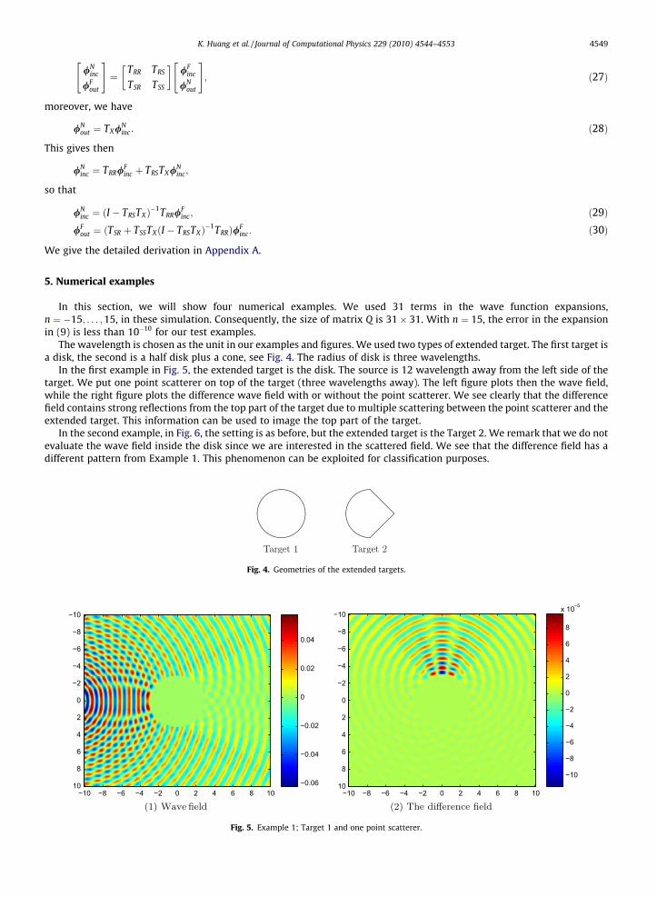
In the first example in Fig. 5, the extended target is the disk. The source is 12 wavelength away from the left side of thetarget. We put one point scatterer on top of the target (three wavelengths away). The left figure plots then the wave field,while the right figure plots the difference wave field with or without the point scatterer. We see clearly that the differencefield contains strong reflections from the top part of the target due to multiple scattering between the point scatterer and theextended target. This information can be used to image the top part of the target.

In the second example, in Fig. 6, the setting is as before, but the extended target is the Target 2. We remark that we do notevaluate the wave field inside the disk since we are interested in the scattered field. We see that the difference field has adifferent pattern from Example 1. This phenomenon can be exploited for classification purposes.

Fig. 4. Geometries of the extended targets.

−10 −8 −6 −4 −2 0 2 4 6 8 10

10

−8

−6

−4

−2

0

2

4

6

8

10 −0.06

−0.04

−0.02

0

0.02

0.04

−10 −8 −6 −4 −2 0 2 4 6 8 10

−10

−8

−6

−4

−2

0

2

4

6

8

10−10

−8

−6

−4

−2

0

2

4

6

8

x 10−5

Fig. 5. Example 1; Target 1 and one point scatterer.

−10 −8 −6 −4 −2 0 2 4 6 8 10

−10

−8

−6

−4

−2

0

2

4

6

8

10 −0.06

−0.04

−0.02

0

0.02

0.04

−10 −8 −6 −4 −2 0 2 4 6 8 10

−10

−8

−6

−4

−2

0

2

4

6

8

10 −3

−2

−1

0

1

2

3x 10−4

Fig. 6. Example 2; Target 2 and one point scatterer.

−10 −8 −6 −4 −2 0 2 4 6 8 10

−10

−8

−6

−4

−2

0

2

4

6

8

10 −0.08

−0.06

−0.04

−0.02

0

0.02

0.04

0.06

0.08

−10 −8 −6 −4 −2 0 2 4 6 8 10

−10

−8

−6

−4

−2

0

2

4

6

8

10 −0.03

−0.02

−0.01

0

0.01

0.02

0.03

Fig. 7. Example 3; Target 2 and 200 point scatterers.

−10 −8 −6 −4 −2 0 2 4 6 8 10

−10

−8

−6

−4

−2

0

2

4

6

8

10−6

−4

−2

0

2

4

6

x 10−3

−10 −8 −6 −4 −2 0 2 4 6 8 10

−10

−8

−6

−4

−2

0

2

4

6

8

10 −8

−6

−4

−2

0

2

4

6

x 10−5

Fig. 8. Example 4. Source in far field.

4550 K. Huang et al. / Journal of Computational Physics 229 (2010) 4544–4553

In the third example, in Fig. 7, we randomly put 200 point scatterers surrounding the Target 2. In this case the differencefield corresponding to specular reflection from the target and scattering from the tip of the cone (as in the previous example)

K. Huang et al. / Journal of Computational Physics 229 (2010) 4544–4553 4551

is relatively strongest. We remark that with our approach we can easily handle a large number of point scatterers, e.g.thousands.

In the last example, in Fig. 8, the source is 1000 wavelengths away from the Target 2. There are 10 random point scattererssurrounding the target. Note how the difference field gives information about the location of the point targets and also infor-mation about the geometry of the extended target via the point scatterers. The example illustrates that we easily can resolvefar field phenomena. The main computation is the formation of the matrix Q, in which we used adaptive Simpsonquadrature.

We conclude that we have been able to calculate the scattered fields in the Foldy-Lax formulation in the presence of anextended scatterer, a situation corresponding to a strong separation of scales and where using discretization of the Helm-holtz equation would have been very expensive.

6. Conclusion

We have developed an efficient numerical algorithm to simulate multiple scattering among point scatterers and extendedtargets in 2D. In our algorithm the free space Green’s function is used and no partial differential equations need to be dis-cretized and solved. The main computational cost is the formation of the matrix Q. In our approach we can easily deal withlong propagation distances and large number of point scatterers. Extension to 3D is being studied.

Acknowledgment

The research is partially supported by ONR Grant N00014-05-1-0442.

Appendix A. Generalized Foldy–Lax system

In this appendix, we derive the generalized Foldy–Lax formulation that gives the exciting field at the extended scattererand the point scatterer. The excited field can then be used to compute the scattered field at any point in the domain.

Let the exciting field at the scatterers be denoted by

/Ej ¼ /ðrjÞ; 1 6 j 6 N:

The impinging (far field) source field may for instance be generated by a set of point sources. We write it as in (19):

wFincðrÞ ¼

Xn

/FincðnÞRnðrÞ:

The incoming field on S2, see Fig. 3, is now

/incðrÞ ¼X1

n¼�1RnðrÞ/F

incðnÞ þXN

j¼1

rj/Ej gðr; rjÞ ¼

X1n¼�1

RnðrÞ/FincðnÞ þ i

XN

j¼1

rj/Ej

X1n¼�1

SnðrjÞRnðrÞ

¼X1

n¼�1/F

incðnÞ þXN

j¼1

Anj/Ej

!RnðrÞ ¼ RðrÞ � ð/F

inc þ A/EÞ;

with

Anj ¼ irjSnðrjÞ:

We then use (7) and (11) to find for r 2 S2

ð/Finc þ A/EÞ � RðrÞ ¼ i

Xm

bm

ZS

ds0X1

n¼�1½Snðr0Þn̂ � r0Rmðr0Þ�RnðrÞ ¼ iQb � RðrÞ;

and in view of the orthogonality of the cylindrical harmonics

/Finc þ A/E ¼ iQb; ð31Þ

which generalizes the relation (12).Next, let jrj > maxr2Sjrj and write the field scattered by the extended scatterer as

/scaðrÞ ¼X1

n¼�1f Xn SnðrÞ;

then we have as in (15)

fX ¼ �iRealðQ Þb;

with b defined as in (11). In view of (31) we then find

4552 K. Huang et al. / Journal of Computational Physics 229 (2010) 4544–4553

fX ¼ �RealðQ ÞQ�1ð/Finc þ A/EÞ: ð32Þ

The exciting field at the scatterers can now be identified as

/Ej ¼ RðrjÞ � /F

inc þXN

l¼1–j

rlgðrj; rlÞ/El þ

X1n¼�1

f Xn SnðrjÞ; 1 6 j 6 N:

We write these relations in the form

Z/E ¼ C/Finc þ PfX

; ð33Þ

for Z defined in (3) and

Cjn ¼ RnðrjÞ; Pjn ¼ SnðrjÞ:

From (32) and (33) we then find

fX ¼ �RealðQ ÞQ�1ð/Finc þ AZ�1ðC/F

inc þ PfXÞÞ;

so that

fX ¼ ½Iþ RealðQ ÞQ�1AZ�1P��1ð�RealðQ ÞQ�1ðIþ AZ�1CÞÞ/Finc:

Recall the operators introduced in Fig. 3 and below:

TRR ¼ Iþ AZ�1C;

TX ¼ �RealðQ ÞQ�1;

TRS ¼ AZ�1P;

then we have

fX ¼ ½I� TXTRS��1TXTRR /Finc ¼ TX ½I� TRSTX ��1TRR /F

inc:

Finally, we derive the expression for the scattered field that is generated by the exciting field at both the point scatterers andthe extended scatterer. Let the point of field evaluation, r, be such that jrj > maxjjrjj. The field generated by the exciting fieldat the scatters is

/Psca ¼

XN

j¼1

/Ej rjgðr; rjÞ ¼

XN

j¼1

/Ej rj

X1n¼�1

iSnðrÞRnðrjÞ ¼X1

n¼�1

XN

j¼1

Hnj/Ej

!SnðrÞ �

X1n¼�1

f Pn SnðrÞ;

for

Hnj ¼ irjRnðrjÞ:

The total scattered wave-field coefficients are then

fX þ fP ¼ fTX ½I� TRSTX ��1TRR /Finc þHZ�1ðC/F

inc þ PfXÞg ¼ fTX ½I� TRSTX ��1TRR þHZ�1CþHZ�1PTX ½I� TRSTX ��1TRRg/Finc:

We again use a notation as in Fig. 3:

/Fout ¼ fX þ fP

;

TSS ¼ IþHZ�1P; TSR ¼ HZ�1C;

to obtain

/Fout ¼ ðTSR þ TSSTX ½I� TRSTX ��1TRRÞ/F

inc;

which is (30).We finally turn our interest to the total field impinging on the extended scatterer. We write for r < minjjrjj

/incðrÞ ¼X1

n¼�1/N

incðnÞRnðrÞ

and have then

/Ninc ¼ ð/

Finc þ A/EÞ ¼ ð/F

inc þ AZ�1C/Finc þ AZ�1PTX ½I� TRSTX ��1TRR /F

incÞ ¼ ðTRR þ TRSTX ½I� TRSTX ��1TRRÞ/Finc

¼ ½I� TRSTX ��1TRR/Finc;

which is (29).

K. Huang et al. / Journal of Computational Physics 229 (2010) 4544–4553 4553

References

[1] R.H.T. Bates, D.J.N. Wall, Null field approach to scalar diffraction, I. General methods, II. Approximation methods, Philos. Trans. R. Soc. Lond. A287(1977) 45–95.

[2] J.C. Bolomey, A. Wirgin, Numerical comparison of the Green’s function and the Waterman and Rayleigh theories of scattering from a cylinder, Proc. IEE121 (1974) 794–804.

[3] M. Born, E. Wolf, Principles of Optics, Academic Press, New York, 1970.[4] D. Colton, R. Kress, Inverse Acoustic and Electromagnetic Scattering Theory, Springer, 1998.[5] L.L. Foldy, The multiple scattering of waves, Phys. Rev. 67 (1945) 107–119.[6] M. Lax, Multiple scattering of waves, Rev. Mod. Phys. 23 (1951) 287–310.[7] M. Lax, Multiple scattering of waves II. The effective field in dense systems, Phys. Rev. 85 (1952) 261–269.[8] Leung Tsang, Jin-Au Kong, Kung-Hau Ding, Chi-On Ao, Scattering of electromagnetic waves, Numerical Simulations, John Wiley & Sons, Inc.,, New York,

2001.[9] P.C. Waterman, New formulation of acoustic scattering, J. Acoust. Soc. Am. 45 (1969) 1417–1429.

[10] P.C. Waterman, Symmetry, unitarity and geometry in electromagnetic scattering, Phys. Rev. D 3 (4) (1971) 825–829.[11] Weng Cho Chew, Waves and Fields in Inhomogeneous Media, Van Nostrand Reinhold, New York, 1990.