Generalized Additive Model

by

Huimin Liu

Department of Mathematics and Statistics University of Minnesota Duluth, Duluth, MN 55812

December 2008

1

Table of Contents Abstract…………………...………………………………………………………………2 Chapter 1 Introduction

1.1 RegressionReview …………………………………………………………….3 1.2 Introduce to Generalized Additive Model (GAM) ……………...……………4

Chapter 2 Smoothing 2.1 What it a Smoother……………………………………………………...…….5 2.2 Cubic Smoothing Splines……………………………………...………...…….5 2.3 Automatic selection of smoothing parameter ………………………………8 2.3.1 From MSE to PSE……………………………………………….......8 2.3.2 Cross Validation…………………………………………………....10 2.3.3 Generalized Cross Validation……………………………………...12 2.3.4 Degrees of Freedom of a Smoother…………………………..……15 Chapter 3 Generalized Additive Model (GAM) 3.1 Generalized Additive Model (GAM)………………………………………...17 3.2 Fitting Generalized Additive Model…………………………………………17 3.3 The Logistic Generalized Additive Model………………………………......21 Chapter 4 Examples 4.1 Example 1: Comparing GAM with GLM…………………….….………… 25 4.2 Example 2: Fitting logistic GAM model using GAM procedure……………28

Chapter 5 Discussion……………………………………………………………………………….35 References……………...………………………………………………………………..36 Appendix………………………………………………………………………………...37

2

Abstract

Generalized linear model assumes a linear relationship between the mean of the

dependent variable and the unknown parameter . or

, where are independent variables. In this paper, we

study the class of Generalized Additive models [Hastie and Tibshirani. (1990)], which

replace the linear form by a sum of smooth functions . This non-

parametric function can be estimated in a flexible manner using cubic spline

smoother, in an iterative method called the back fitting algorithm. Generalized Additive

models are suitable for exploring the data set and visualizing the relationship between the

dependant variable and the independent variables. This paper illustrates the technique by

comparing the PROC GAM procedure with the PROC GLM procedure by using SAS and

uses PROC GAM to model data from binary distribution as well.

Keywords:

Generalized Additive Models (GAM), cubic spline smoother, non-parametric, back-

fitting

3

Chapter 1 Introduction

1.1 Regression Review

One of the most popular and useful tools in data analysis is the linear regression model. It

is a statistical technique used for modeling and analysis of numerical data consisting of

values of a dependent variable and of one or more independent variables.

Let Y be a dependent (response) variable, and be p independent (predictor or

regressor) variables. Our goal is to describe the dependence of the mean of Y as a

function of . For this purpose, we assume that the mean of Y is a linear function

of ,

or for some function g. (1.1.1)

Given a sample of values for Y and X, where , the estimates of

are often obtained by the least squares method. It is achieved by fitting a

linear model which minimizes , where .

4

1.2 Introduction to the Generalized Additive Model (GAM)

The Generalized additive model replaces with where is an

unspecified (‘non-parametric’) function. It can be in a non-linear form:

(1.2.1)

This function is estimated in a flexible manner using cubic spline smoother.

5

Chapter 2 Smoothing

2.1 What is a Smoother?

A smoother is a tool for summarizing the trend of a dependent variable Y as a function of

one or more independent variables . It produces an estimate of the trend that is

less variable than Y itself; hence named smoother. We call the estimate produced by a

smoother a smooth.

Smoother is very useful in statistical analysis. First, we can pick out the trend from the

plot easily. Second, it estimates the dependence of the mean of Y on the predictors.

The most important property of smoother is its non-parametric nature. So the smooth

function is also known as non-parametric function. It doesn’t assume a rigid form for the

dependence of Y on . This is the biggest difference from Generalized Linear

Model (GLM). It allowes an ‘approximation’ with sum of functions, (these functions

have separated input variables), not just with one unknown function only. That’s why it is

the building block of the generalized additive model algorithm.

2.2 Cubic Smoothing Splines

A cubic spline smoother is a solution to the following optimization problem: among all

functions with second continuous derivatives, find one that minimizes the

penalized least square, which called cubic spline smoother.

6

(2.2.1)

where is a fixed constant, and . In the subsequent chapters, I

assume includes all possible range.

The name cubic spline is from the piecewise polynomial fit, with the order k=3, where

most study shown that k=3 is sufficient.

Note that the first term represents the least square method. With only this part, the result

would be an interpolated curve that would not be smooth at all. It measures closeness to

the data while the second term penalizes curvature in the function. measures

the ‘wiggliness’ of the function . Linear functions have , while non-

linear functions produce non-zero values.

is a non-negative smoothing parameter that must be chosen by the data analyst. It

governs the tradeoff between the goodness of fit to the data and the wiggleness of the

function. It plays nearly the same role as span (the percentage of data points used as

nearest neighbors in percent of total n) in other smoothing methods. When , the

penalty term becomes more important, forcing , thus the result is the least

square line. When , the penalty becomes unimportant, thus a solution is the

second derivative function. The larger values of produce smoother curves while the

7

smaller values produce more wiggly curves. How to choose the appropriate will be

discussed in the following section.

In order to see it clearly, I will describe cubic smoothing splines in a simple setting.

Suppose that we have a scattleplot of points shown in Figure 2.2.1.

Figure 2.1

Figure 2.2

8

Figure 2.3

Figure 2.2.1 shows a scatterplot of an outcome that measures y by plotting it against an

independent variables x. In Figure 2.2.2, the straight line was fitted by least square

method. In Figure 2.2.3, a cubic spline has been added to describe the trend of y on x.

Visually, we can see that the cubic smoothing spline describe the trend of y as a function

of x better than the least square method.

2.3 Automatic Selection of Smoothing Parameters

2.3.1 From MSE to PSE

In order to minimize the cubic spline smoother, we have to choose the smoothing

parameter. To do this, we don’t need to minimize the Mean Square Error at each , but

instead we focus on a global measure such as Average Mean Square Error (AMSE)

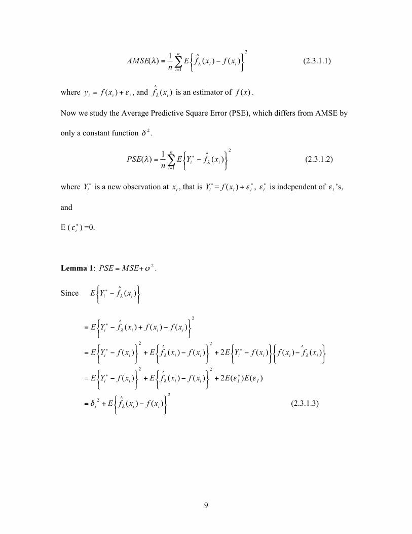
9

(2.3.1.1)

where , and is an estimator of .

Now we study the Average Predictive Square Error (PSE), which differs from AMSE by

only a constant function .

(2.3.1.2)

where is a new observation at , that is = , is independent of ’s,

and

E ( ) =0.

Lemma 1: .

Since

10

Then

Based on the proof, it turned out that one can estimate PSE rather than MSE, which is

more appropriate and achievable.

2.3.2 Cross Validation

Cross-Validation is the statistical method of partitioning a sample of data into two

subsets, a training (calibration) subset for modeling fitting and a test (validation) subset

for model evaluation. This approach, however, is not efficient unless the sample is large.

The idea behind cross-validation is to recycle data by switching the roles of training and

test samples.

During the practice, in order to simplify and not to waste the data set, we are more

interested in the Leave-one-out Cross-validation. As the name suggests, the leave-one-out

cross-validation (LOOCV) works by leaving the point out one at a time as the

testing set and estimating the smooth at base on the remaining points.

11

One then constructs the Cross-validation sum of squares. (Sometimes called jackknifed

fit at )

(2.3.2.1)

where indicates the fit at computed by leaving out the ith data point.

Using the same idea that was used in the last section,

Here =0, because doesn’t involve yi.

Moreover if, we assume ,

12

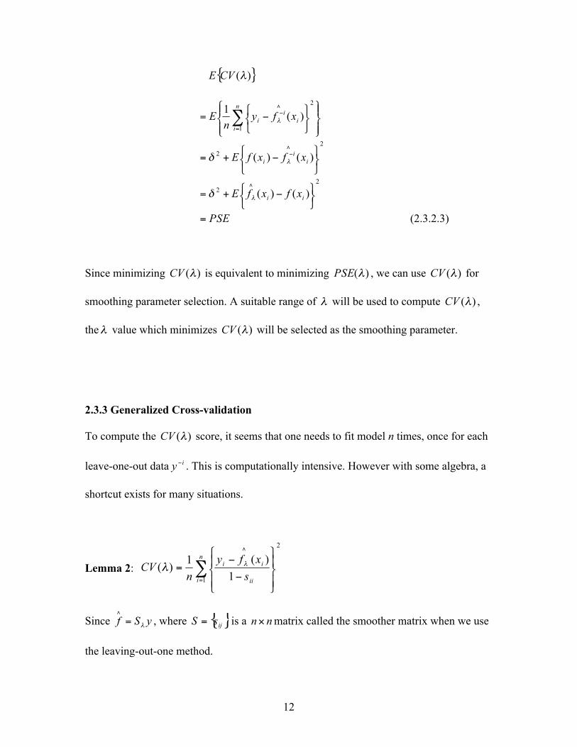
Since minimizing is equivalent to minimizing , we can use for

smoothing parameter selection. A suitable range of will be used to compute ,

the value which minimizes will be selected as the smoothing parameter.

2.3.3 Generalized Cross-validation

To compute the score, it seems that one needs to fit model n times, once for each

leave-one-out data . This is computationally intensive. However with some algebra, a

shortcut exists for many situations.

Lemma 2:

Since , where is a matrix called the smoother matrix when we use

the leaving-out-one method.

13

Let

(2.3.3.1)

Then (2.3.3.2)

(2.3.3.3)

Combine Equations (2.3.3.2) and (2.3.3.3) we have

(2.3.3.4)

Then

(2.3.3.5)

Thus . (2.3.3.6)

14

Thus the fit can be computed from and . There is no need to actually

remove the ith point and re-compute the smooth. We only need to fit model once with the

full data and compute the diagonal elements of the smother matrix.

If we replace by the averages of all the diagonal elements, it results in the following

Generalized Cross Validation (GCV).

(2.3.3.7)

GCV is a weighted version of CV with weights .

If is small, using the approximation , then

(2.3.3.8)

If we regard in the second part as an estimate of , the GCV is

approximately the same as statistics.

Statistics (2.3.3.9)

15

Thus GCV can be used to obtain the minimal smoothing parameter. Show below is an

example of how the smoothing parameter is chosen by GCV function using SAS.

Figure 2.4

Figure 2.4 is the plot of the GCV function vs. . The GCV function has two

minima. The plot shows a minimum at 1.1. The figure also suggests a local minimum

around -4.2. Note that the SAS procedure for GCV function may not always find the

global minimum, though it did in this case. We can calculate the corresponding to be

about 0.11. In this case the degree of freedom is about 8.8.

2.3.4 Degrees of Freedom of a Smoother

In fact it is inconvenient to express the desired smoothness of functions in terms of . In

the SAS GAM procedure, we also select the value of a smoothing parameter simply by

specifying the df for the smoother.

16

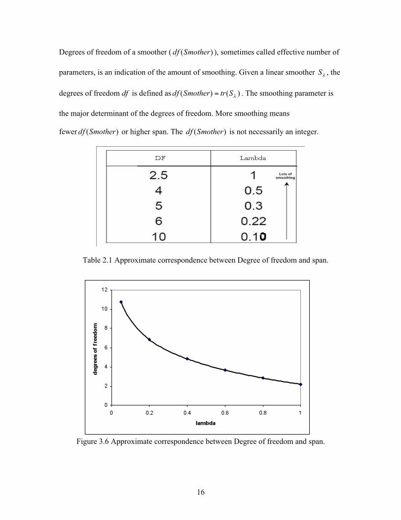
Degrees of freedom of a smoother ( ), sometimes called effective number of

parameters, is an indication of the amount of smoothing. Given a linear smoother , the

degrees of freedom df is defined as . The smoothing parameter is

the major determinant of the degrees of freedom. More smoothing means

fewer or higher span. The is not necessarily an integer.

Table 2.1 Approximate correspondence between Degree of freedom and span.

Figure 3.6 Approximate correspondence between Degree of freedom and span.

17

Chapter 3 Generalized Additive Model (GAM)

3.1 Generalized Additive Model (GAM)

The generalized additive model (GAM) is a statistical model developed by Hastie and

Tibshirani in the year 1990. It is applicable in many areas of prediction.

An additive model has the form

(3.1.1)

where the errors are independent of the ’s, and . The ’s

are arbitrary univariate functions, one for each variable.

3.2 Fitting the Generalized Additive Model

There are a number of approaches for the formulation and estimation of additive models.

The back-fitting algorithm is a general algorithm that can fit an additive model using any

regression-type fitting mechanism.

Define the jth set of partial residuals as

(3.2.1)

then . This observation provides a way for estimating each

smoothing function .

18

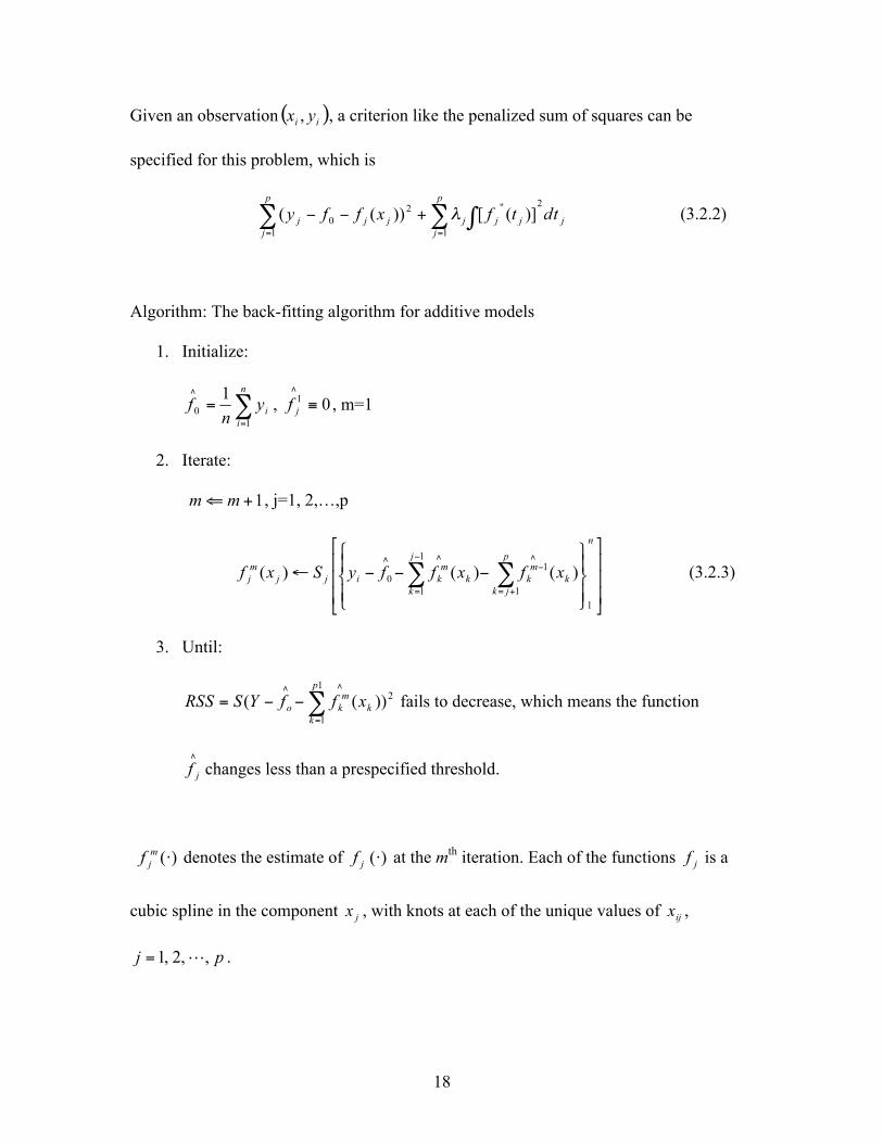
Given an observation , a criterion like the penalized sum of squares can be

specified for this problem, which is

(3.2.2)

Algorithm: The back-fitting algorithm for additive models

1. Initialize:

, , m=1

2. Iterate:

, j=1, 2,…,p

(3.2.3)

3. Until:

fails to decrease, which means the function

changes less than a prespecified threshold.

denotes the estimate of at the mth iteration. Each of the functions is a

cubic spline in the component , with knots at each of the unique values of ,

.

19

The GAM procedure uses the following condition as the convergence criterion for the

backfitting algorithm:

(3.2.4)

where by default.

Now let’s take a look at the Back-fitting Algorithm in details.

When m = 1 + 1 = 2, j = 1

= (3.2.5)

where does not exist, since the upper limit is smaller than the

lower limit.

By applying a cubic smoothing spline to the targets , as a function of , we

will obtain a new estimate .

20

When j = 2

= (3.2.6)

By repeating this, we can estimate , all of the smoothing functions at the 2nd

iteration.

Then goes to next iteration, m = 2 + 1 = 3. j = 1

(3.2.7)

where has already been found in the last cycle, does not

exist.

By doing the same thing as m = 2 in the 2nd iteration, this time we will find the .

Keep iterating and we will find all the smoothing functions.

21

3.3 The Generalized Additive Logistic Model

Far binary data, the most popular approach is logistic regression,

let where is a vector of covariates.

and (3.3.1)

In logistic GAM, the basic idea is to replace the linear predictor with an additive one:

and (3.3.2)

Generally, let , .

(3.3.3)

where is a function of p variables.

Assume Y= , given some initial estimate of , construct the adjusted

dependent variable

(3.3.4)

22

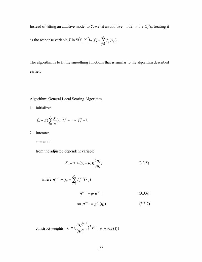
Instead of fitting an additive model to Y, we fit an additive model to the ’s, treating it

as the response variable Y in .

The algorithm is to fit the smoothing functions that is similar to the algorithm described

earlier.

Algorithm: General Local Scoring Algorithm

1. Initialize:

,

2. Interate:

m = m + 1

from the adjusted dependent variable

(3.3.5)

where

(3.3.6)

so (3.3.7)

construct weights ,

23

Fit a weighted additive model to to obtain estimated function , additive

predictor , and fitted value

3. Until:

Repeat step 2, until the change deviance is sufficiently small.

(3.3.8)

or compute (3.3.9)

The GAM procedure uses the following condition as the convergence criterion for the

back-fitting algorithm:

(3.3.10)

where by default.

Given some initial estimations of , a first order Taylor series expansion, together

with the fisher scoring method, will give the improved estimate

(3.3.11)

24

(3.3.12)

(3.3.13)

(3.3.14)

(3.3.15)

Since and

so (3.3.16)

(3.3.17)

so (3.3.18)

25

(3.3.19)

Then replace the conditional estimations by smoothers

(3.3.20)

Chapter 4 Examples

4.1 Example 1: Comparing the GAM and the GLM

In SAS, the PROC GAM procedure in SAS implements the Generalized Additive Model

and the PROC GLM procedure fits the Generalized Liner Model.

In an analysis of a simulation from a chemistry experiment, Generalized Additive Model

fitted by the PROC GAM procedure is compared to the Generalized Linear Model fitted

by using the PROC GLM procedure.

The data set consists of 3 variables. They are measurements of the temperature of the

experiment, the amount of catalyst added, and the yield of the chemical reaction. Here the

yield is the response variable.

26

Temperature Catalyst Yield

80 0.005 6.039

80 0.010 4.719

80 0.015 6.301

… … …

90 0.005 4.540

90 0.010 3.553

… … …

140 0.080 6.006

Table 4.1: Sample data set for example 1.

The following plots were generated by SAS.

Figure 4.1 Plot of the raw data.

27

Figure 4.2 The predicted plane fitted by the GLM procedure.

Figure 4.3 The predicted surface fitted by the GAM procedure.

28

Figure 4.1 is the surface plot of Yield by Temperature and Amount of Catalyst of the raw

data. Figure 4.2 is the plane fitted by using the PROC GLM procedure. Figure 4.3 is the

surface fitted by the PROC GAM. Clearly the predicted surface using the GAM

procedure produces much better prediction results.

4.2 Example 2: Fitting Logistic GAM Model using the GAM Procedure

The data used in this example are based on a study of chronic bronchitis in Cardiff

conducted by Jones(1975). The data in the study consist of observations on three

variables for each of 212 men in a Cardiff districts sample. The variables are CIG, the

number of cigarettes smoked per day, POLL, the smoke level in the locality of the

respondent’s home (obtained by interpolation from 13 air pollution monitoring stations

on the city), and R, an indicator variable taking the value 1 if the respondent suffered

from chronic bronchitis, and 0 if he did not.

Data Description

R Chronic Bronchitis (1=presence, 0=absence)

CIG

Cigarette Consumption

POLL Smoke Level of Locality of

Respondents Home

0 5.15 67.1

1 0.0 66.9

0 2.5 66.7

0 1.75 65.8

29

0 6.75 64.4

0 0.0 64.4

… … …

0 0.9 55.4

Table 4.2: Sample data set for example 2.

The first step of data exploration is to visualize the distribution of numeric predictors.

Empirical distribution of variables CIG and POLL were estimated with kernel density

estimation using the KDE procedure in SAS and were shown in Figure 4.4.

Figure 4.4 Distributions of CIG and POLL Clearly, both numeric predictors are skewed to the left, as shown in Figure 4.4.

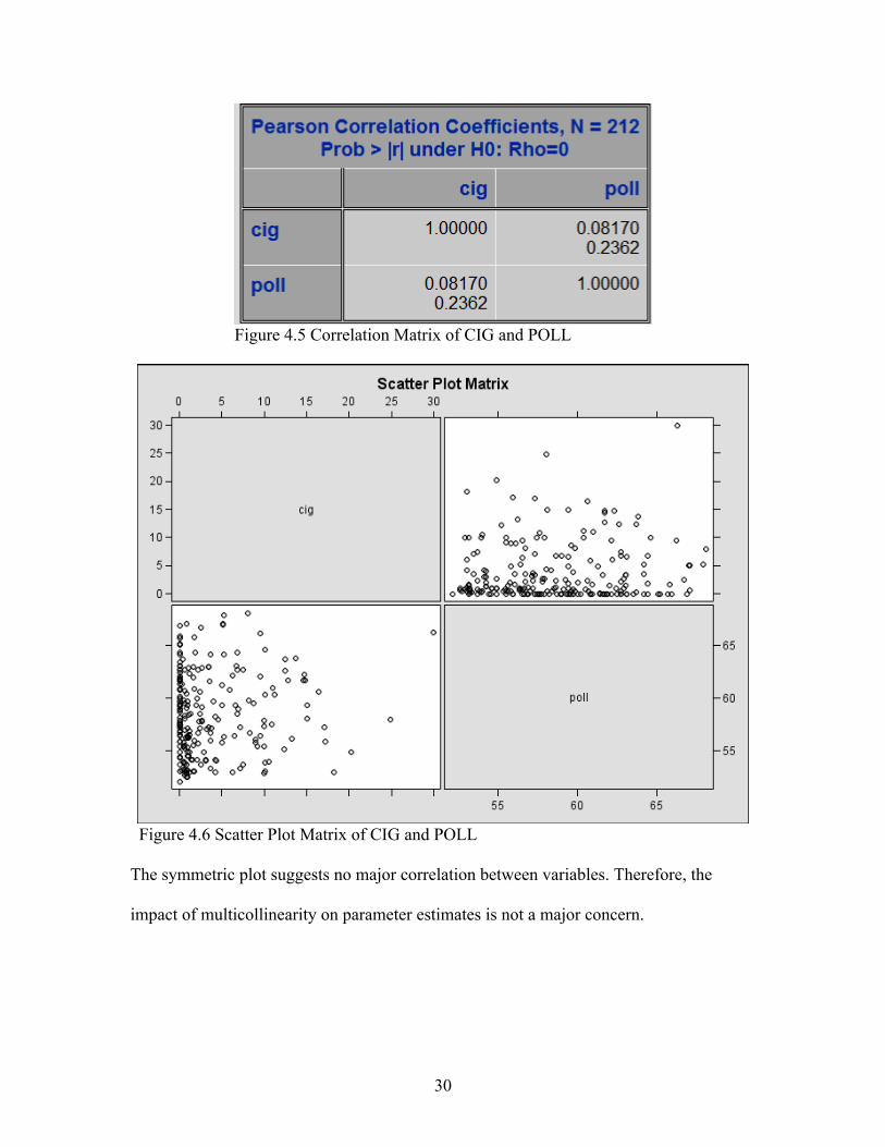
The correlations between numeric predictors are also investigated using the CORR

procedure in SAS and the result is presented in Figure 4.5 and Figure 4.6.

30

Figure 4.5 Correlation Matrix of CIG and POLL

Figure 4.6 Scatter Plot Matrix of CIG and POLL The symmetric plot suggests no major correlation between variables. Therefore, the

impact of multicollinearity on parameter estimates is not a major concern.

31

Modeling

PROC GAM procedure was then used to fit a model, with flexible spline terms for each

of the predictors. In this model, we choose df = 3. Of these three degrees of freedom, one

is taken up by the linear portion of the fit and the other two are left for the nonlinear

spline portion. Although this might seem to be a modest amount of flexibility, it is better

to use this number with a small data set. This avoids over-fitting and lower the

computing cost.

Parts of the SAS outputs from the PROC GAM procedure are listed in Figures 4.7, 4.8,

4.9 and Figure 4.10.

Figure 4.7 Summary for the input data and algorithms

32

Figure 4.8 Analytical information about the fitted model

Figure 4.9 Analysis of Deviance

The first part of the output from the PROC GAM procedure (Figure 4.7) summarizes the

input data set and provides a summary for the bac-kfitting and local scoring algorithms.

The second part of the output (Figure 4.8) provides the analytical information about the

fitted model.

The critical part of the output is the “Analysis of Deviance” Table, shown in Figure 4.7.

For each smoothing effect in the model, this table gives a Chi-square test comparing the

33

deviance between the full model and the model without this variable. In this case, the

analysis of deviance results indicated that the effects of CIG is significant, while POLL is

insignificant at 5% level.

Figure 4.8 Partial Prediction for Each Predictor

The plots show that the partial predictions corresponding to both CIG and POLL have a

quadratic pattern. Note that the 95% confidence limits for the Poll contains the zero axis,

confirming the insignificance of this term.

The GAM procedure generated the following output (Figure 4.9), including the predicted

logit and predicted probability. The predicted logit is not of direct interest. Use inverse

link function to convert logit to probability. For example, when the number of cigarettes

smoked per day is 5.15 and the smoke level in the locality of the respondent’s home

equals 67.1, according to the Logistic GAM estimated from the data, the probability of

suffering from chronic bronchitis is 0.51881.

34

Figure 4.9 Partial output of Logistic Generalized Additive Model P_bronchitis is the predicted logit. Phat represents the predicted probability.

35

Chapter 5 Discussion

Generalized additive models provide a flexible method for uncovering nonlinear

relationship between dependent and independent variables in exponential family and

other likelihood based regression models. In the two data examples given in this paper,

the iterative method called the back-fitting algorithm was used to predict the unspecified

function. The cublic spline smoother was applied to the independent variables.

36

References:

1. Hasties, T.J. and Tibshirani, R.J. (1990), Generalized Additive MODELS, New York:

Chapman and Hall.

2. Friedman, J., Hasties, T.J. and Tibshirani, R.J. (2000), Additive logistic regression: a

statistical view of boosting, The Annals of Statistics 2000, Vol. 28, No. 2,337-407.

3. Dong, X. (2001), Fitting Generalized Additive Models with the GAM procedure,

SUGI Proceedings.

4. Wood, Simon N. Generalized Additive Model: an introduction with R, Chapman and

Hall/CRC.

5. Friedman, J. (1991), Multivariate adaptive regression splines, Annals of Statistics

19(1), 1-141.

6. Marx, Brain D. and Eilers, Paul H.C (1998), Direct generalized additive modeling

with pernalized likelihood, Computational Statistics and Data Analysis 28(1998) 193-

209.

7. Liu, Wensui and Cela, Jimmy (2007), Improving credit scoring by generalized

additive model, SAS global forum 2007 (paper 078-2007)

8. http://en.wikipedia.org/wiki/Generalized_additive_model

37

Appendix SAS Code

A. SAS Code Used to Choose the Smoothing Parameter by GCV.

data bronchitis;

infile ‘bronchitis.dat’;

input bronchitis cig poll @@;

run;

proc tpspline data=bronchitis;

ods output GCVFunction=gcv;

model bronchitis = (cig poll) /lognlambda=(-6 to 1 by 0.1);

run;

symbol1 interpol=join value=none;

title "GCV Function";

proc gplot data=gcv;

plot gcv*lognlambda/frame cframe=ligr

vaxis=axis1 haxis=axis2;

run;

38

B. SAS Code Used to compare PROC GAM with PROC GLM.

********************************************************************

*1.This SAS program use PROC G3D to fit the surface plot of the raw*

*data set. The raw data set include three numeric variables: two *

*horizontal variables plotted on the x and y axes the difine an x-y*

*plane, and a vertical variable plotted on the z axis rising from *

*the {it x-y}plane. *

*2.Fit models with PROC GLM and PROC GAM. *

*3.Plot predict yield value from both GLM and GAM models agaist *

* temperature and catalyst. *

********************************************************************

ods pdf;

ods graphics on;

libname here '.';

data ExperimentA;

infile ‘ExperimentA.dat;

format Temperature f4.0 Catalyst f6.3 Yield f8.3;

input Temperature Catalyst Yield @@;

ods graphics on;

title2 'Raw data';

proc g3d data=ExperimentA;

plot Temperature*Catalyst=Yield

/ zmin=2 zmax=11;

run;

proc glm;

model Yield=Temperature Catalyst;

output out=here.a p=pred;

run

Proc Print data=here.a;

run;

39

proc g3d data=here.a;

format pred f6.3;

plot Temperature*Catalyst=pred

/ name= 'GLM' zmin=2 zmax=11;

run;

proc gam data=ExperimentA;

model Yield = loess(Temperature) loess(Catalyst)

/ method=gcv;

output out=PredGAM;

run;

proc g3d data=PredGLM;

format P_Yilde f6.3;

plot Temperature*Catalyst=P_Yield

/ name= 'GLM' zmin=2 zmax=11;

run;

goptions display;

proc greplay nofs tc=sashelp.templt template=v2;

igout=gseg;

treplay 1:GAMA 2:GLM;

run;

quit;

ods graphics off;

ods pdf close;

40

C. SAS Code Used to fit Logistic GAM model using PROC GAM procedure.

ods html;

ods graphics on;

/* Input data set*/

data bronchitis;

input bronchitis cig poll @@;

datalines;

0 5.15 67.1 1 0.0 66.9 0 2.5 66.7 0 1.75 65.8

0 6.75 64.4 0 0.0 64.4 1 0.0 65.1 1 9.5 66.2

0 0.0 65.9 0 0.75 67.1 0 5.25 67.9 1 8 68.1

1 5.15 67 1 30.0 66.3 0 0.0 65.7 0 0.0 65.2

0 5.25 64.2 0 10.05 64.6 0 0.0 63.5 1 3.4 63.0

0 0.0 62.7 0 .55 62.7 1 9.5 62.1 1 12.5 63.7

0 0.0 63.1 0 3.4 63 0 2.2 62.7 0 6.7 63.1

0 1.1 62.4 0 1.8 64.4 0 0.0 64.2 1 3.6 64.2

0 1.6 63 0 6.2 62.2 0 14.75 62.3 0 .35 63.7

1 13.75 63.8 0 0.0 63.1 1 7.5 62.7 0 1.0 62.9

0 0.0 62.5 1 14.8 61.7 1 3.5 61.6 0 0.0 61.6

0 0.0 61.4 0 .25 61.4 0 1.55 62 1 0.0 61.8

0 0.0 60.9 0 5.9 60.8 0 16.45 60.6 0 2.65 62.9

1 12.5 62.6 0 0.0 62.1 0 14.55 61.7 1 11 61

1 6.75 62.7 0 0.0 62.7 1 0.0 61.7 0 1.75 60.9

0 2.4 60.6 0 10.05 60.4 1 12.75 61.7 0 0.0 61.9

0 5 61.3 0 .6 60.7 0 0.0 60.8 0 .85 60.5

0 .9 59.7 0 .0 59.5 1 8.75 59.6 0 .8 59.1

1 6.6 59.4 0 1.0 58.5 0 0.0 60 1 8.15 59.8

0 0.0 59.7 1 5 59.4 0 2.55 59.2 0 1.2 58.6

0 0.0 60.8 1 11.25 60.4 0 0.0 60.2 0 2 60

0 1.9 59.4 0 .45 59.8 1 0.0 59.7 0 0.0 59.0

1 6.9 59.0 0 2.35 58.6 0 3.95 59.7 0 .6 59.6

1 15 59.4 0 0.0 59.4 0 .95 59.4 0 0.0 59.3

0 1.4 54.2 0 .5 54.0 0 .6 53.8 0 0.0 53.7

0 2.45 53.7 0 1.75 53.1 0 0.0 54.4 0 3.1 54.2

0 10.05 53.9 0 .55 53.2 0 .85 53.2 0 1.1 54.9

0 0.0 54.9 0 0.0 54.5 0 1.45 54.2 0 2.05 54.2

1 10.5 54 0 .5 55.8 1 9.2 55.5 0 .55 55.6

0 0.0 55.5 0 0.96 54.9 0 1 54.6 0 0.0 56.9

0 5.25 56.4 1 0 55.9 0 9 55.8 0 1.6 55.6

1 10.9 57.6 0 0.0 57.7 0 0 57.6 0 2.25 57.8

41

0 2.65 57.8 0 .55 58.4 0 0 58.2 1 4.5 58

0 15 58.1 0 0 57.9 0 0 57.3 0 4.2 58.3

0 .55 58.1 1 10 57.9 0 0 57.6 0 7.1 57.3

0 3.2 57.1 1 0 58.9 1 6.8 58.6 0 0 58.7

0 0 57.5 0 2.35 57.2 0 24.9 58 0 2.65 57.9

1 3.7 57.2 0 17.1 57.3 0 0 57.5 0 .95 57.2

0 10.05 53.1 0 1.15 53 1 18.25 53 0 10 52.9

0 .75 52.6 0 0 53.1 0 4.2 53 0 .8 52.9

0 .55 52.7 0 .95 52.6 0 0 52.1 0 3.1 54.1

0 .8 53.7 0 1.55 53.1 0 .4 53.3 0 6.2 53

0 .6 53 0 .4 53.9 1 7.5 53.7 0 7.15 53.4

0 .25 53.2 0 3.6 53.4 0 .95 53.2 0 2.8 54.9

1 20.25 54.9 0 .95 54.6 0 4.25 54.1 0 4.15 54.2

0 10 57.4 0 3.4 57.3 0 0.0 57.3 0 3.6 56.7

0 .9 56.5 0 0.0 56.8 0 0 56.6 1 6.4 56.5

0 .95 56.3 0 1.06 56.3 0 13.3 56.2 0 1.1 56.6

0 17.2 55.9 0 1.65 56 1 5 55.8 0 2.1 55.7

0 .6 57 1 8.25 56.7 0 .9 56.4 0 0.0 56.5

1 12.3 55.2 0 1.15 56.9 0 2.2 56.7 0 3.6 56

1 10 55.5 0 0.6 55.3 0 9.5 56.5 0 .7 56.3

1 9 56.1 0 0 55.9 0 .5 55.5 0 .9 55.4

;

proc kde data=bronchitis;

bivar cig poll/plot=all;

run;

proc corr data=bronchitis plots=matrix;

var cig poll;

run;

/*Fitting the Logistic GlM*/

proc logistic data=bronchitis;

model bronchitis=cig poll/ link=logit

scale=none

clparm=wald

clodds=pl

rsquare

outroc=roc;

42

run;

proc print data=pred_bronchitis;

run;

symbol1 i=join v=none c=blue;

proc gplot data=roc;

plot _sensit_*_1mspec_=1/ vaxis= 0 to 1 by 0.1 ;

run;

/*Fitting the Logistic GAM*/

proc gam data=bronchitis plots(clm);

model bronchitis = spline(cig,df=3) spline(poll,df=3)

/dist=binomial r outroc=roc;

output out=pred_bronshitis all;

run;

proc print data=pred_bronshitis;

data bphat;

infile ‘pred_bronshitis.dat’

input Obs bronchitis cig poll P_bronchitis P_cig P_poll @@;

phat=exp(P_bronchitis)/(1+exp(P_bronchitis));

proc print data=bphat (keep=Obs bronchitis cig poll P_bronchitis

phat);

run;

symbol1 i=join v=none c=blue;

proc gplot data=roc;

plot _sensit_*_1mspec_=1/ vaxis= 0 to 1 by 0.1 ;

run;

ods graphics off;

ods html close;