Generalization and Equilibrium in Generative Adversarial Nets

(GANs)

Sanjeev Arora∗ Rong Ge † Yingyu Liang‡ Tengyu Ma§ Yi Zhang¶

Abstract

We show that training of generative adversarial network (GAN) may not have good general-ization properties; e.g., training may appear successful but the trained distribution may be farfrom target distribution in standard metrics. However, generalization does occur for a weakermetric called neural net distance. It is also shown that an approximate pure equilibrium ex-ists1 in the discriminator/generator game for a special class of generators with natural trainingobjectives when generator capacity and training set sizes are moderate.

This existence of equilibrium inspires mix+gan protocol, which can be combined with anyexisting GAN training, and empirically shown to improve some of them.

1 Introduction

Generative Adversarial Networks (GANs) [Goodfellow et al., 2014] have become one of the dominantmethods for fitting generative models to complicated real-life data, and even found unusual usessuch as designing good cryptographic primitives [Abadi and Andersen, 2016]. See a survey byGoodfellow [2016]. Various novel architectures and training objectives were introduced to addressperceived shortcomings of the original idea, leading to more stable training and more realisticgenerative models in practice (see Odena et al. [2016], Huang et al. [2017], Radford et al. [2016],Tolstikhin et al. [2017], Salimans et al. [2016], Jiwoong Im et al. [2016], Durugkar et al. [2016] andthe reference therein).

The goal is to train a generator deep net whose input is a standard Gaussian, and whose outputis a sample from some distribution D on Rd, which has to be close to some target distribution Dreal(which could be, say, real-life images represented using raw pixels). The training uses samplesfrom Dreal and together with the generator net also trains a discriminator deep net trying tomaximise its ability to distinguish between samples from Dreal and D. So long as the discriminatoris successful at this task with nonzero probability, its success can be used to generate a feedback

∗Princeton University, Computer Science Department, email: arora@cs.princeton.edu†Duke University, Computer Science Department, email: rongge@cs.duke.edu‡Princeton University, Computer Science Department, email: yingyul@cs.princeton.edu§Princeton University, Computer Science Department, email: tengyu@cs.princeton.edu¶Princeton University, Computer Science Department, email: yz7@cs.princeton.edu1This is an updated version of an ICML’17 paper with the same title. The main difference is that in the ICML’17

version the pure equilibrium result was only proved for Wasserstein GAN. In the current version the result applies tomost reasonable training objectives. In particular, Theorem 4.3 now applies to both original GAN and WassersteinGAN.

1

arX

iv:1

703.

0057

3v5

[cs

.LG

] 1

Aug

201

7

Figure 1: Probability density Dreal with many peaks and valleys

(using backpropagation) to the generator, thus improving its distribution D. Training is continueduntil the generator wins, meaning that the discriminator can do no better than random guessingwhen deciding whether or not a particular sample came from D or Dreal. This basic iterativeframework has been tried with many training objectives; see Section 2. But it has been unclearwhat to conclude when the generator wins this game: is D close to Dreal in some metric? One seemsto need some extension of generalization theory that would imply such a conclusion. The hurdle isthat distribution Dreal could be complicated and may have many peaks and valleys; see Figure 1.The number of peaks (modes) may even be exponential in d. (Recall the curse of dimensionality:in d dimensions there are exp(d) directions whose pairwise angle exceeds say π/3, and each couldbe the site of a peak.) Whereas the number of samples from Dreal (and from D for that matter)used in the training is a lot fewer, and thus may not reflect most of the peaks and valleys of Dreal.

A standard analysis due to [Goodfellow et al., 2014] shows that when the discriminator capacity(= number of parameters) and number of samples is “large enough”, then a win by the generatorimplies that D is very close to Dreal (see Section 2). But the discussion in the previous paragraphraises the possibility that “sufficiently large” in this analysis may need to be exp(d).

Another open theoretical issue is whether an equilibrium always exists in this game betweengenerator and discriminator. Just as a zero gradient is a necessary condition for standard opti-mization to halt, the corresponding necessary condition in a two-player game is an equilibrium.Conceivably some of the instability often observed while training GANs could just arise because oflack of equilibrium. (Recently Arjovsky et al. [2017] suggest that using their Wasserstein objectivein practice reduces instability, but we still lack proof of existence of an equilibrium.) Standard gametheory is of no help here because we need a so-called pure equilibrium, and simple counter-examplessuch as rock/paper/scissors show that it doesn’t exist in general2.

1.1 Our Contributions

We formally define generalization for GANs in Section 3 and show that for previously studiednotions of distance between distributions, generalization is not guaranteed (Lemma 1). In factwe show that the generator can win even when D and Dreal are arbitrarily far in any one of thestandard metrics.

However, we can guarantee some weaker notion of generalization by introducing a new metricon distributions, the neural net distance. We show that generalization does happen with moderatenumber of training examples (i.e., when the generator wins, the two distributions must be close in

2Such counterexamples are easily turned into toy GAN scenarios with generator and discriminator having finitecapacity, and the game lacks a pure equilibrium. See Appendix C.

2

neural net distance). However, this weaker metric comes at a cost: it can be near-zero even whenthe trained and target distributions are very far (Section 3.4).

To explore the existence of equilibria we turn in Section 4 to infinite mixtures of generator deepnets. These are clearly vastly more expressive than a single generator net: e.g., a standard result inbayesian nonparametrics says that every probability density is closely approximable by an infinitemixture of Gaussians [Ghosh et al., 2003]. Thus unsurprisingly, an infinite mixture should win thegame. We then prove rigorously that even a finite mixture of fairly reasonable size can closelyapproximate the performance of the infinite mixture (Theorem 4.2).

This insight also allows us to construct a new architecture for the generator network where thereexists an approximate equilibrium that is pure. (Roughly speaking, an approximate equilibrium isone in which neither of the players can gain much by deviating from their strategies.) This existenceproof for an approximate equilibrium unfortunately involves a quadratic blowup in the “size” of thegenerator (which is still better than the naive exponential blowup one might expect). Improvingthis is left for future theoretical work. But we propose a heuristic approximation to the mixtureidea to introduce a new framework for training that we call MIX+GAN. It can be added on top ofany existing GAN training procedure, including those that use divergence objectives. Experimentsin Section 6 show that for several previous techniques, MIX+GAN stabilizes the training, and insome cases improves the performance.

2 Preliminaries

Notations. Throughout the paper we use d for the dimension of samples, and p for the numberof parameters in the generator/discriminator. In Section 3 we use m for number of samples.

Generators and discriminators. Let Gu, u ∈ U (U ⊂ Rp) denote the class of generators, whereGu is a function — which is often a neural network in practice — from R` → Rd indexed by u thatdenotes the parameters of the generators. Here U denotes the possible ranges of the parametersand without loss of generality we assume U is a subset of the unit ball3. The generator Gu definesa distribution DGu as follows: generate h from `-dimensional spherical Gaussian distribution andthen apply Gu on h and generate a sample x = Gu(h) of the distribution DGu . We drop thesubscript u in DGu when it’s clear from context.

Let Dv, v ∈ V denote the class of discriminators, where Dv is function from Rd to [0, 1] andv is the parameters of Dv.

Training the discriminator consists of trying to make it output a high value (preferably 1) whenx is sampled from distribution Dreal and a low value (preferably 0) when x is sampled from thesynthetic distribution DGu . Training the discriminator consists of trying to make its syntheticdistribution “similar”to Dreal in the sense that the discriminator’s output tends to be similar onthe two distributions.

We assume Gu and Dv are L-Lipschitz with respect to their parameters. That is, for all u, u′ ∈ Uand any input h, we have ‖Gu(h)−Gu′(h)‖ ≤ L‖u− u′‖ (similar for D).

Notice, this is distinct from the assumption (which we will also sometimes make) that functionsGu, Dv are Lipschitz: that focuses on the change in function value when we change x, while keepingu, v fixed4.

3Otherwise we can scale the parameter properly by changing the parameterization.4Both Lipschitz parameters can be exponential in the number of layers in the neural net, however our Theorems

3

Objective functions. The standard GAN training [Goodfellow et al., 2014] consists of trainingparameters u, v so as to optimize an objective function:

minu∈U

maxv∈V

Ex∼Dreal

[logDv(x)] + Ex∼DGu

[log(1−Dv(x))]. (1)

Intuitively, this says that the discriminator Dv should give high values Dv(x) to the real samplesand low values Dv(x) to the generated examples. The log function was suggested because of itsinterpretation as the likelihood, and it also has a nice information-theoretic interpretation describedbelow. However, in practice it can cause problems since log x→ −∞ as x→ 0. The objective stillmakes intuitive sense if we replace log by any monotone function φ : [0, 1] → R, which yields theobjective:

minu∈U

maxv∈V

Ex∼Dreal

[φ(Dv(x))] + Ex∼DGu

[φ(1−Dv(x))]. (2)

We call function φ the measuring function. It should be concave so that when Dreal and DG arethe same distribution, the best strategy for the discriminator is just to output 1/2 and the optimalvalue is 2φ(1/2). In later proofs, we will require φ to be bounded and Lipschitz. Indeed, in practicetraining often uses φ(x) = log(δ + (1 − δ)x) (which takes values in [log δ, 0] and is 1/δ-Lipschitz)and the recently proposed Wasserstein GAN [Arjovsky et al., 2017] objective uses φ(x) = x.Training with finite samples. The objective function (2) assumes we have infinite numberof samples from Dreal to estimate the value Ex∼Dreal [φ(Dv(x))]. With finite training examplesx1, . . . , xm ∼ Dreal, one uses 1

m

∑mi=1[φ(Dv(xi))] to estimate the quantity Ex∼Dreal [φ(Dv(x))]. We

call the distribution that gives 1/m probability to each of the xi’s the empirical version of the realdistribution. Similarly, one can use a empirical version to estimate Ex∼DGu [φ(1−Dv(x))].Standard interpretation via distance between distributions. Towards analyzing GANs,researchers have assumed access to infinite number of examples and that the discriminator ischosen optimally within some large class of functions that contain all possible neural nets. Thisoften allows computing analytically the optimal discriminator and therefore removing the maximumoperation from the objective (2), which leads to some interpretation of how and in what sense theresulting distribution DG is close to the true distribution Dreal.

Using the original objective function (1), then the optimal choice among all the possible func-

tions from Rd → (0, 1) is D(x) = Preal(x)Preal(x)+PG(x) , as shown in Goodfellow et al. [2014]. Here Preal(x)

is the density of x in the real distribution, and PG(x) is the density of x in the distribution gener-ated by generator G. Using this discriminator — though it’s computationally infeasible to obtainit — one can show that the minimization problem over the generator correspond to minimizing theJensen-Shannon (JS) divergence between the true distribution Dreal and the generative distributionDG. Recall that for two distributions µ and ν, the JS divergence is defined by

dJS(µ, ν) =1

2(KL(µ‖µ+ ν

2) +KL(ν‖µ+ ν

2)) .

Other measuring functions φ and choice of discriminator class leads to different distance func-tion between distribution other than JS divergence. Notably, Arjovsky et al. [2017] shows thatwhen φ(t) = t, and the discriminator is chosen among all 1-Lipschitz functions, maxing out thediscriminator, the generator is attempting to minimize the Wasserstein distance between Dreal and

only depend on the log of the Lipschitz parameters

4

Du(h). Recall that Wasserstein distance between µ and ν is defined as

dW (µ, ν) = supD is 1-Lipschitz

∣∣∣∣ Ex∼µ[D(x)]− Ex∼ν

[D(x)]

∣∣∣∣ .3 Generalization theory for GANs

The above interpretation of GANs in terms of minimizing distance (such as JS divergence andWasserstein distance) between the real distribution and the generated distribution relies on twocrucial assumptions: (i) very expressive class of discriminators such as the set of all boundeddiscriminator or the set of all 1-Lipschitz discriminators, and (ii) very large number of examples tocompute/estimate the objective (1) or (2). Neither assumption holds in practice, and we will shownext that this greatly affects the generalization ability, a notion we introduce in Section 3.1.

3.1 Definition of Generalization

Our definition is motivated from supervised classification, where training is said to generalize if thetraining and test error closely track each other. (Since the purpose of GANs training is to learna distribution, one could also consider a stronger definition of successful training, as discussed inSection 3.4.)

Let x1, . . . , xm be the training examples, and let Dreal denote the uniform distribution overx1, . . . , xm. Similarly, let Gu(h1), . . . , Gu(hr) be a set of r examples from the generated distributionDG. In the training of GANs, one implicitly uses Ex∼Dreal [φ(Dv(x))] to approximate the quantityEx∼Dreal [φ(Dv(x))]. Inspired by the observation that the training objective of GANs and its variantsis to minimize some distance (or divergence) d(·, ·) between Dreal and DG using finite samples, wedefine the generalization of GANs as follows:

Definition 1. Given Dreal, an empirical version of the true distribution with m samples, a gener-ated distribution DG generalizes under the divergence or distance between distributions d(·, ·) withgeneralization error ε if the following holds with high probability5,∣∣∣d(Dreal,DG)− d(Dreal, DG)

∣∣∣ ≤ ε (3)

where and DG is an empirical version of the generated distribution DG with polynomial number ofsamples (drawn after DG is fixed).

In words, generalization in GANs means that the population distance between the true andgenerated distribution is close to the empirical distance between the empirical distributions. Ourtarget is to make the former distance small, whereas the latter one is what we can access andminimize in practice. The definition allows only polynomial number of samples from the generateddistribution because the training algorithm should run in polynomial time.

We also note that stronger versions of Definition 1 can be considered. For example, as an analogof uniform convergence in supervised learning, we can require (3) to hold for all generators DGamong a class of candidate generators. Indeed, our results in Section 3.3 show that all generatorsgeneralize under neural net distance with reasonable number of examples.

5over the choice of DG

5

3.2 JS Divergence and Wasserstein don’t Generalize

As a warm-up, we show that JS divergence and Wasserstein distance don’t generalize with anypolynomial number of examples because the population distance (divergence) is not reflected bythe empirical distance.

Lemma 1. Let µ be uniform Gaussian distributions N (0, 1dI) and µ be an empirical versions of µ

with m examples. Then we have dJS(µ, µ) = log 2, dW (µ, µ) ≥ 1.1.

There are two consequences of Lemma 1. First, consider the situation where Dreal = DG = µ.Then we have that dW (Dreal,DG) = 0 but dW (Dreal, DG) > 1 as long as we have polynomialnumber of examples. This violates the generalization definition equation (3).

Second, consider the case Dreal = µ and DG = Dreal = µ, that is, DG memorizes all of thetraining examples in Dreal. In this case, since DG is a discrete distribution with finite supports,with enough (polynomial) examples, in DG, effectively we also have that DG ≈ DG. Therefore, wehave that dW (Dreal, DG) ≈ 0 whereas dW (Dreal,DG) > 1. In other words, with any polynomialnumber of examples, it’s possible to overfit to the training examples using Wasserstein distance.The same argument also applies to JS divergence. See Appendix B.1 for the formal proof. Notice,this result does not contradict the experiments of Arjovsky et al. [2017] since they actually use notWasserstein distance but a surrogate distance that does generalize, as we show next.

3.3 Generalization bounds for neural net distance

Which distance measure between Dreal and DG is the GAN objective actually minimizing and canwe analyze its generalization performance? Towards answering these questions in full generality(given multiple GANs objectives) we consider the following general distance measure that unifiesJS divergence, Wasserstein distance, and the neural net distance that we define later in this section.

Definition 2 (F-distance). Let F be a class of functions from Rd to [0, 1] such that if f ∈ F , 1−f ∈F . Let φ be a concave measuring function. Then the F-divergence with respect to φ between twodistributions µ and ν supported on Rd is defined as

dF ,φ(µ, ν) = supD∈F

Ex∼µ

[φ(D(x))] + Ex∼ν

[φ(1−D(x))]− 2φ(1/2)

When φ(t) = t, we have that dF ,φ is a distance function 6 , and with slightly abuse of notation wewrite it simply as dF (µ, ν) = supD∈F |Ex∼µ[D(x)]− Ex∼ν [D(x)]| .

Example 1. When φ(t) = log(t) and F = all functions from Rd to [0, 1], we have that dF ,φ isthe same as JS divergence. When φ(t) = t and F = all 1-Lipschitz functions from Rd to [0, 1],then dF ,φ is the Wasserstein distance.

Example 2. Suppose F is a set of neural networks and φ(t) = log t, then original GAN objectivefunction is equivalent to minG dF ,φ(Dreal, DG) .

Suppose F is the set of neural networks, and φ(t) = t, then the objective function used empiri-cally in Arjovsky et al. [2017] is equivalent to minG dF (Dreal, DG) .

6Technically it is a pseudometric. This is also known as integral probability metrics[Muller, 1997].

6

GANs training uses F to be a class of neural nets with a bound p on the number of parameters.We then informally refer to dF as the neural net distance. The next theorem establishes generaliza-tion in the sense of equation (3) does hold for it (with a uniform convergence) . We assume that themeasuring function takes values in [−∆,∆] and that it is Lφ-Lipschitz. Further, F = Dv, v ∈ Vis the class of discriminators that is L-Lipschitz with respect to the parameters v. As usual, we usep to denote the number of parameters in v.

Theorem 3.1. In the setting of previous paragraph, let µ, ν be two distributions and µ, ν be em-pirical versions with at least m samples each. There is a universal constant c such that when

m ≥ cp∆2 log(LLφp/ε)

ε2, we have with probability at least 1− exp(−p) over the randomness of µ and ν,

|dF ,φ(µ, ν)− dF ,φ(µ, ν)| ≤ ε.

See Appendix B.1 for the proof. The intuition is that there aren’t too many distinct discrim-inators, and thus given enough samples the expectation over the empirical distribution convergesto the expectation over the true distribution for all discriminators.

Theorem 3.1 shows that the neural network divergence (and neural network distance) has amuch better generalization properties than Jensen-Shannon divergence or Wasserstein distance.If the GAN successfully minimized the neural network divergence between the empirical distri-butions, that is, d(Dreal, DG), then we know the neural network divergence d(Dreal,DG) betweenthe distributions Dreal and DG is also small. It is possible to change the proof to also show thatthis generalization continues to hold at every iteration of the training as shown in the followingcorollary.

Corollary 3.1. In the setting of Theorem 3.1, suppose G(1), G(2), ..., G(K) (logK d) be the Kgenerators in the K iterations of the training, and assume logK ≤ p. There is a some universal

constant c such that when m ≥ cp∆2 log(LLφp/ε)

ε2, with probability at least 1−exp(−p), for all t ∈ [K],∣∣∣dF ,φ(Dreal,DG(t))− dF ,φ(Dreal, DG(t))

∣∣∣ ≤ ε .The key observation here is that the objective is separated into two parts and the generator

is not directly related to Dreal. So even though we don’t have fresh examples, the generalizationbound still holds. Detailed proof appears in Appendix B.1.

3.4 Generalization vs Diversity

Since the final goal of GANs training is to learn a distribution, it is worth understanding thatthough weak generalization in the sense of Section 3.3 is guaranteed, it comes with a cost. For JSdivergence and Wasserstein distance, when the distance between two distributions µ, ν is small, itis safe to conclude that the distributions µ and ν are almost the same. However, the neural netdistance dNN (µ, ν) can be small even if µ, ν are not very close. As a simple Corollary of Lemma 3.1,we obtain:

Corollary 3.2 (Low-capacity discriminators cannot detect lack of diversity). Let µ be the empiricalversion of distribution µ with m samples. There is a some universal constant c such that when

m ≥ cp∆2 log(LLφp/ε)

ε2, we have that with probability at least 1− exp(−p), dF ,φ(µ, µ) ≤ ε.

7

That is, the neural network distance for nets with p parameters cannot distinguish betweena distribution µ and a distribution with support O(p/ε2). In fact the proof still works if thedisriminator is allowed to take many more samples from µ; the reason they don’t help is that itscapacity is limited to p.

We note that similar results have been shown before in study of pseudorandomness [Trevisanet al., 2009] and model criticism [Gretton et al., 2012].

4 Expressive power and existence of equilibrium

Section 3 clarified the notion of generalization for GANs: namely, neural-net divergence betweenthe generated distribution D and Dreal on the empirical samples closely tracks the divergence onthe full distribution (i.e., unseen samples). But this doesn’t explain why in practice the generatorusually “wins”so that the discriminator is unable to do much better than random guessing at theend. In other words, was it sheer luck that so many real-life distributions Dreal turned out to beclose in neural-net distance to a distribution produced by a fairly compact neural net? This sectionsuggests no luck may be needed.

The explanation starts with a thought experiment. Imagine allowing a much more powerfulgenerator, namely, an infinite mixture of deep nets, each of size p. So long as the deep net classis capable of generating simple gaussians, such mixtures are quite powerful, since a classical resultsays that an infinite mixtures of simple gaussians can closely approximate Dreal. Thus an infinitemixture of deep net generators will “win” the GAN game, not only against a discriminator that isa small deep net but also against more powerful discriminators (e.g., any Lipschitz function).

The next stage in the thought experiment is to imagine a much less powerful generator, whichis a mix of only a few deep nets, not infinitely many. Simple counterexamples show that now thedistribution D will not closely approximate arbitrary Dreal with respect to natural metrics like `p.Nevertheless, could the generator still win the GAN game against a deep net of bounded capacity(i.e., the deep net is unable to distinguish D and Dreal)? We show it can.

informal theorem: If the discriminator is a deep net with p parameters, then a mixture ofO(p log(p/ε)/ε2) generator nets can produce a distribution D that the discriminator will be unableto distinguish from Dreal with probability more than ε. (Here O(·) notation hides some nuisancefactors.)

This informal theorem is also a component of our result below about the existence of an approx-imate pure equilibrium. We will first show that a finite mixture of generators can “win” againstall discriminators, and then discuss how this mixed generator can be realized as a single generatornetwork that is 1-layer deeper.

4.1 Equilibrium using a Mixture of Generators

For a class of generators Gu, u ∈ U and a class of discriminators Dv, v ∈ V, we can define thepayoff F (u, v) of the game between generator and discriminator

F (u, v) = Ex∼Dreal

[φ(Dv(x))] + Ex∼DG

[φ(1−Dv(x)))]. (4)

Of course as we discussed in previous section, in practice these expectations should be with respectto the empirical distributions. Our discussions in this section does not depend on the distributionsDreal and Dh, so we define F (u, v) this way for simplicity.

8

The well-known min-max theorem [v. Neumann, 1928] in game theory shows if both players areallowed to play mixed strategies then the game has a min-max solution. A mixed strategy for thegenerator is just a distribution Su supported on U , and one for discriminator is a distribution Svsupported on V.

Theorem 4.1 (von Neumann). There exists a value V , and a pair of mixed strategies (Su,Sv) suchthat

∀v, Eu∼Su

[F (u, v)] ≤ V and ∀u, Ev∼Sv

[F (u, v)] ≥ V.

Note that this equilibrium involves both parties announcing their strategies Su,Sv at the start,such that neither will have any incentive to change their strategy after studying the opponent’sstrategy. The payoff is generated by the generator first sample u ∼ Su, h ∼ Dh, and then generatean example x = Gu(h). Therefore, the mixed generator is just a linear mixture of generators. Amixture of discriminators is more complicated because the objective function need not be linearin the discriminator. However in the case of our interest, the generator wins and even a mixtureof discriminators cannot effectively distinguish between generated and real distribution. Thereforewe do not consider a mixture of discriminators here.

Of course, this equilibrium involving an infinite mixture makes little sense in practice. Weshow that (as is folklore in game theory [Lipton and Young, 1994]) that we can approximate thismin-max solution with mixture of finitely many generators and discriminators. More precisely wedefine ε-approximate equilibrium:

Definition 3. A pair of mixed strategies (Su,Sv) is an ε-approximate equilibrium, if for some valueV

∀v ∈ V, Eu∼Su

[F (u, v)] ≤ V + ε;

∀u ∈ U , Ev∼Sv

[F (u, v)] ≥ V − ε.

If the strategies Su,Sv are pure strategies, then this pair is called an ε-approximate pure equilibrium.

Suppose φ is Lφ-Lipschitz and bounded in [−∆,∆], the generator and discriminators are L-Lipschitz with respect to the parameters and L′-Lipschitz with respect to inputs, in this setting wecan formalize the above Informal Theorem as follows:

Theorem 4.2. In the settings above, if the generator can approximate any point mass7, there is

a universal constant C > 0 such that for any ε, there exists T =C∆2p log(LL′Lφ·p/ε)

ε2generators

Gu1 , . . . GuT . Let Su be a uniform distribution on ui, and D is a discriminator that outputs only1/2, then (Su, D) is an ε-approximate equilibrium.

The proof uses a standard probabilistic argument and epsilon net argument to show that if wesample T generators and discriminators from infinite mixture, they form an approximate equilib-rium with high probability. For the second part, we use the fact that the generator can approximateany point mass, so an infinite mixture of generators can approximate the real distribution Dreal towin. Therefore indeed a mixture of O(p) generators can achieve an ε-approximate equilibrium.

Note that this theorem works for a wide class of measuring functions φ (as long as φ is concave).The generator always wins, and the discriminator’s (near) optimal strategy corresponds to randomguessing (output a constant 1/2).

7For all points x and any ε > 0, there is a generator such that Eh∼Dh [‖G(h)− x‖] ≤ ε.

9

4.2 Achieving Pure Equilibrium

Now we give a construction to augment the network structure, and achieve an approximate pureequilibrium for the GAN game for generator nets of size O(p2). This should be interpreted as: ifdeep nets of size p are capable of generating any point mass, then the GAN game for the generatorneural network of size O(p2) has an approximate equilibrium in which the generator wins. (Thetheorem is stated for RELU gates but also holds for standard activations such as sigmoid.)

Theorem 4.3. Suppose the generator and discriminator are both k-layer neural networks (k ≥ 2)with p parameters, and the last layer uses ReLU activation function. In the setting of The-orem 4.2, there exists k + 1-layer neural networks of generators G and discriminator D with

O(

∆2p2 log(LL′Lφ·p/ε)ε2

)parameters, such that there exists an ε-approximate pure equilibrium with

value 2φ(1/2).

To prove this theorem, we consider the mixture of generators as in Theorem 4.2, and show howto fold the mixture into a larger k + 1-layer neural network. We sketch the idea; details are in theAppendix B.2.

For mixture of generators, we construct a single neural network that approximately generatesthe mixture distribution using the gaussian input it has. To do that, we can pass the input h throughall the generators Gu1 , Gu2 , ..., GuT . We then show how to implement a “multi-way selector” thatwill select a uniformly random output from DGui (i ∈ [T ]). The selector involves a simple 2-layernetwork that selects a number i from 1 to T with the appropriate probability and “disables”all theneural nets except the ith one by forwarding an appropriate large negative input.

Remark: In practice, GANs use highly structured deep nets, such as convolutional nets. Ourcurrent proof of existence of pure equilibrium requires introducing less structured elements in thenet, namely, the multiway selectors that implement the mixture within a single net. It is left forfuture work whether pure equilibria exist for the original structured architectures. In the meantime,in practice we recommend using, even for W-GAN, a mixture of structured nets for GAN training,and it seems to help in our experiments reported below.

5 MIX+GANs

Theorem 4.2 and Theorem 4.3 show that using a mixture of (not too many) generators and dis-criminators guarantees existence of approximate equilibrium. This suggests that using a mixturemay lead to more stable training. Our experiments correspond to an older version of this paper,and they are done using a mixture for both generator and discriminators.

Of course, it is impractical to use very large mixtures, so we propose mix + gan: use a mixtureof T components, where T is as large as allowed by size of GPU memory (usually T ≤ 5). Namely,train a mixture of T generators Gui , i ∈ [T ] and T discriminators Dvi , i ∈ [T ]) which share thesame network architecture but have their own trainable parameters. Maintaining a mixture meansof course maintaining a weight wui for the generator Gui which corresponds to the probability ofselecting the output of Gui . These weights are also updated via backpropagation. This heuristiccan be combined with existing methods like dcgan, w-gan etc., giving us new training methodsmix+dcgan, mix+w-gan etc.

We use exponentiated gradient [Kivinen and Warmuth, 1997]: store the log-probabilities αui , i ∈

10

[T ], and then obtain the weights by applying soft-max function on them:

wui =eαui∑Tk=1 e

αuk, i ∈ [T ]

Note that our algorithm is maintaining weights on different generators and discriminators. Thisis very different from the idea of boosting where weights are maintained on samples. AdaGAN [Tol-stikhin et al., 2017] uses ideas similar to boosting and maintains weights on training examples.

Given payoff function F , training mix + gan boils down to optimizing:

minui,αui

maxvj,αvj

Ei,j∈[T ]

F (ui, vj)

= minui,αui

maxvj,αvj

∑i,j∈[T ]

wuiwvjF (ui, vj).

Here the payoff function is the same as Equation (4). We use both measuring functions φ(x) = log x(for original GAN) and φ(x) = x (for WassersteinGAN). In our experiments we alternatively updategenerators’ and discriminators’ parameters as well as their corresponding log-probabilities usingADAM [Kingma and Ba, 2015], with learning rate lr = 0.0001.

Empirically, it is observed that some components of the mixture tend to collapse and theirweights diminish during the training. To encourage full use of the mixture capacity, we add to thetraining objective an entropy regularizer term that discourages the weights being too far away fromuniform:

Rent(wui, wvi) = − 1

T

T∑i=1

(log(wui) + log(wvi))

6 Experiments

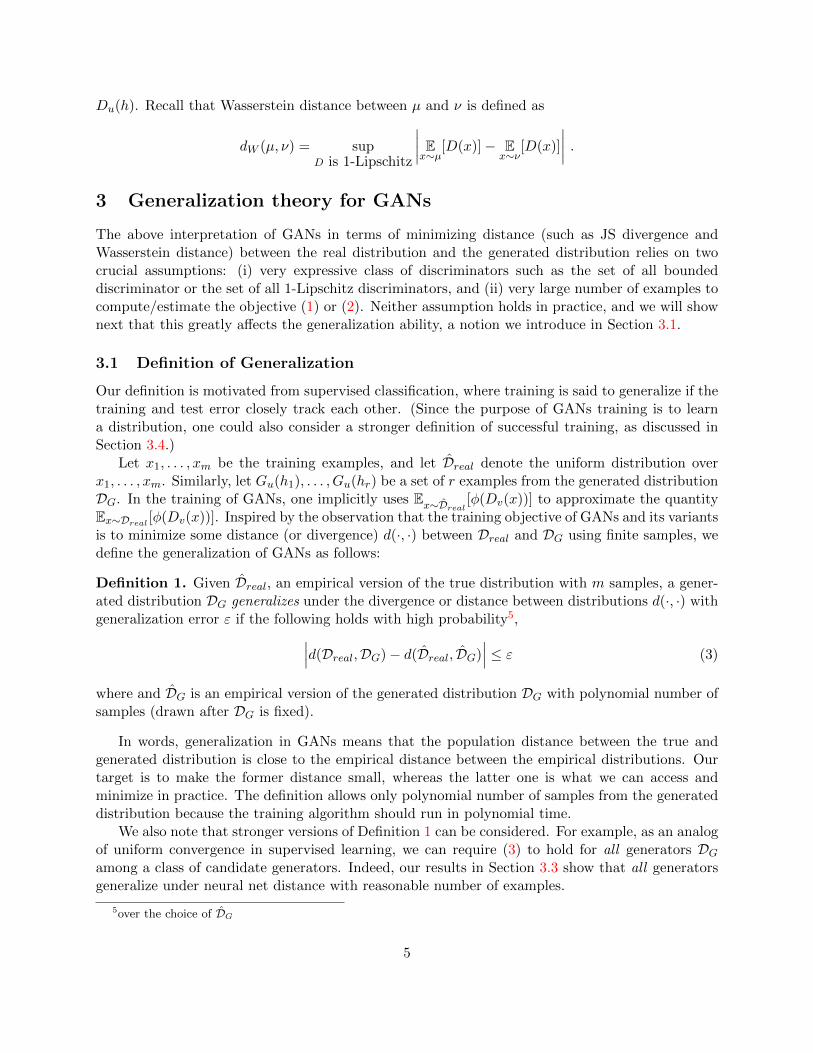
Figure 2: MNIST Samples. Digits generated from (a) MIX+DCGAN and (b) DCGAN.

In this section, we first explore the qualitative benefits of our method on image generation tasks:MNIST dataset [LeCun et al., 1998] of hand-written digits and the CelebA [Liu et al., 2015] dataset

11

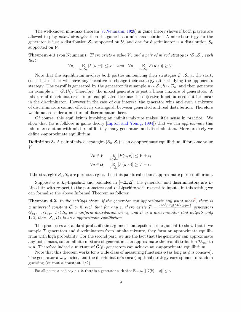
Figure 3: CelebA Samples. Faces generated from (a) MIX+DCGAN and (b) DCGAN.

Table 1: Inception Scores on CIFAR-10. Mixture of DCGANs achieves higher score than anysingle-component DCGAN does. All models except for WassersteinGAN variants are trained withlabels.

Method ScoreSteinGAN [Wang and Liu, 2016] 6.35Improved GAN [Salimans et al., 2016] 8.09±0.07AC-GAN [Odena et al., 2016] 8.25 ± 0.07S-GAN (best variant in [Huang et al., 2017]) 8.59± 0.12DCGAN (as reported in Wang and Liu [2016]) 6.58DCGAN (best variant in Huang et al. [2017]) 7.16±0.10DCGAN (5x size) 7.34±0.07MIX+DCGAN (Ours, with 5 components) 7.72±0.09Wasserstein GAN 3.82±0.06MIX+WassersteinGAN (Ours, with 5 components) 4.04±0.07Real data 11.24±0.12

of human faces. Then for more quantitative evaluation we use the CIFAR-10 dataset [Krizhevskyand Hinton, 2009] and use the Inception Score introduced in Salimans et al. [2016]. MNIST contains60,000 labeled 28×28-sized images of hand-written digits, CelebA contains over 200K 108×108-sizedimages of human faces (we crop the center 64×64 pixels for our experiments), and CIFAR-10 has60,000 labeled 32×32-sized RGB natural images which fall into 10 categories.

To reinforce the point that this technique works out of the box, no extensive hyper-parametersearch or tuning is necessary. Please refer to our code for experimental setup.8

6.1 Qualitative Results

The DCGAN architecture [Radford et al., 2016] uses deep convolutional nets as generators anddiscriminators. We trained mix + dcgan on MNIST and CelebA using the authors’ code as a

8Related code is public online at https://github.com/PrincetonML/MIX-plus-GANs.git

12

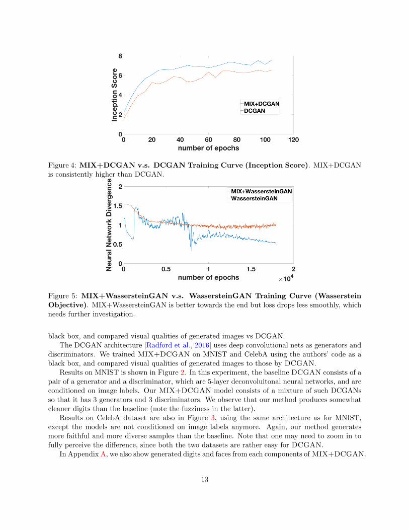
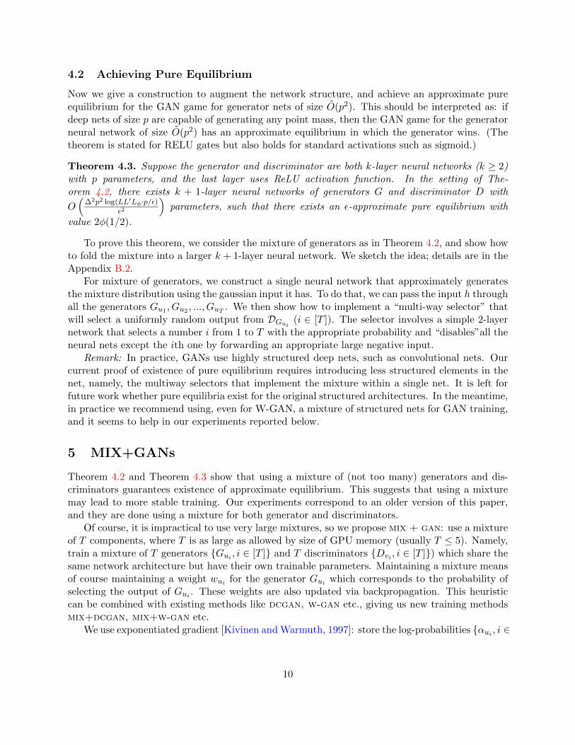
Figure 4: MIX+DCGAN v.s. DCGAN Training Curve (Inception Score). MIX+DCGANis consistently higher than DCGAN.

Figure 5: MIX+WassersteinGAN v.s. WassersteinGAN Training Curve (WassersteinObjective). MIX+WassersteinGAN is better towards the end but loss drops less smoothly, whichneeds further investigation.

black box, and compared visual qualities of generated images vs DCGAN.The DCGAN architecture [Radford et al., 2016] uses deep convolutional nets as generators and

discriminators. We trained MIX+DCGAN on MNIST and CelebA using the authors’ code as ablack box, and compared visual qualities of generated images to those by DCGAN.

Results on MNIST is shown in Figure 2. In this experiment, the baseline DCGAN consists of apair of a generator and a discriminator, which are 5-layer deconvoluitonal neural networks, and areconditioned on image labels. Our MIX+DCGAN model consists of a mixture of such DCGANsso that it has 3 generators and 3 discriminators. We observe that our method produces somewhatcleaner digits than the baseline (note the fuzziness in the latter).

Results on CelebA dataset are also in Figure 3, using the same architecture as for MNIST,except the models are not conditioned on image labels anymore. Again, our method generatesmore faithful and more diverse samples than the baseline. Note that one may need to zoom in tofully perceive the difference, since both the two datasets are rather easy for DCGAN.

In Appendix A, we also show generated digits and faces from each components of MIX+DCGAN.

13

6.2 Quantitative Results

Now we turn to quantitative measurement using Inception Score [Salimans et al., 2016]. Ourmethod is applied to DCGAN and WassersteinGAN Arjovsky et al. [2017], and throughout,mixtures of 5 generators and 5 discriminators are used. At first sight the comparison DCGANv.s. MIX+DCGAN seems unfair because the latter uses 5 times the capacity of the former, withcorresponding penalty in running time per epoch. To address this, we also compare our methodwith larger versions of DCGAN with roughly the same number of parameters, and we found theformer is consistently better than the later, as detailed below.

To construct MIX+DCGAN, we build on top of the DCGAN trained with losses proposedby Huang et al. [2017], which is the best variant so far without improved training techniques. Thesame hyper-parameters are used for fair comparison. See Huang et al. [2017] for more details. Sim-ilarly, for the MIX+WassersteinGAN, the base GAN is identical to that proposed by Arjovskyet al. [2017] using their hyper-parameter scheme.

For a quantitative comparison, inception score is calculated for each model, using 50,000 freshlygenerated samples that are not used in training. To sample a single image from our MIX+ models,we first select a generator from the mixture according to their assigned weights wui, and thendraw a sample from the selected generator.

Table 1 shows the results on the CIFAR-10 dataset. We find that, simply by applying ourmethod to the baseline models, our MIX+ models achieve 7.72 v.s. 7.16 on DCGAN, and 4.04 v.s.3.82 on WassersteinGAN. To confirm that the superiority of MIX+ models is not solely due tomore parameters, we also tested a DCGAN model with 5 times many parameters (roughly thesame number of parameters as a 5-component MIX+DCGAN), which is tuned using a grid searchover 27 sets of hyper-parameters (learning rates, dropout rates, and regularization weights). It getsonly 7.34 (labeled as ”5x size” in Table 1), which is lower than that of a MIX+DCGAN. It isunclear how to apply MIX+ to S-GANs. We tried mixtures of the upper and bottom generatorsseparately, resulting in worse scores somehow. We leave that for future exploration.

Figure 4 shows how Inception Scores of MIX+DCGAN v.s. DCGAN evolve during training.MIX+DCGAN outperforms DCGAN throughout the entire training process, showing that it makeseffective use of the additional capacity.

Arjovsky et al. [2017] shows that (approximated) Wasserstein loss, which is the neural net-work divergence by our definition, is meaningful because it correlates well with visual qualityof generated samples. Figure 5 shows the training dynamics of neural network divergence ofMIX+WassersteinGAN v.s. WassersteinGAN, which strongly indicates that MIX+WassersteinGANis capable of achieving a much lower divergence as well as of improving the visual quality of gen-erated samples.

7 Conclusions

The notion of generalization for GANs has been clarified by introducing a new notion of distancebetween distributions, the neural net distance. (Whereas popular distances such as Wassersteinand JS may not generalize.) Assuming the visual cortex also is a deep net (or some network ofmoderate capacity) generalization with respect to this metric is in principle sufficient to make thefinal samples look realistic to humans, even if the GAN doesn’t actually learn the true distribution.

One issue raised by our analysis is that the current GANs objectives cannot even enforce thatthe synthetic distribution has high diversity (Section 3.4). This is empirically verified in a follow-

14

up work[Arora and Zhang, 2017]. Furthermore the issue cannot be fixed by simply providing thediscriminator with more training examples. Possibly some other change to the GANs setup areneeded.

The paper also made progress another unexplained issue about GANs, by showing that a pureapproximate equilibrium exists for a certain natural training objective (Wasserstein) and in whichthe generator wins the game. No assumption about the target distribution Dreal is needed.

Suspecting that a pure equilibrium may not exist for all objectives, we recommend in practiceour MIX+GAN protocol using a small mixture of discriminators and generators. Our experimentsshow it improves the quality of several existing GAN training methods.

Finally, existence of an equilibrium does not imply that a simple algorithm (in this case, back-propagation) would find it easily. Understanding convergence remains widely open.

Acknowledgements

This paper was done in part while the authors were hosted by Simons Institute. We thank MoritzHardt, Kunal Talwar, Luca Trevisan, Eric Price, and the referees for useful comments. This researchwas supported by NSF, Office of Naval Research, and the Simons Foundation.

15

References

Martın Abadi and David G Andersen. Learning to protect communications with adversarial neuralcryptography. arXiv preprint arXiv:1610.06918, 2016.

Martin Arjovsky, Soumith Chintala, and Leon Bottou. Wasserstein gan. arXiv preprintarXiv:1701.07875, 2017.

Sanjeev Arora and Yi Zhang. Do gans actually learn the distribution? an empirical study. arXivpreprint arXiv:1706.08224, 2017.

I. Durugkar, I. Gemp, and S. Mahadevan. Generative Multi-Adversarial Networks. ArXiv e-prints,November 2016.

Jayanta K Ghosh, RVJK Ghosh, and RV Ramamoorthi. Bayesian nonparametrics. Technicalreport, 2003.

Ian Goodfellow. Nips 2016 tutorial: Generative adversarial networks. arXiv preprintarXiv:1701.00160, 2016.

Ian Goodfellow, Jean Pouget-Abadie, Mehdi Mirza, Bing Xu, David Warde-Farley, Sherjil Ozair,Aaron Courville, and Yoshua Bengio. Generative adversarial nets. In Advances in neural infor-mation processing systems, pages 2672–2680, 2014.

Arthur Gretton, Karsten M Borgwardt, Malte J Rasch, Bernhard Scholkopf, and Alexander Smola.A kernel two-sample test. Journal of Machine Learning Research, 13(Mar):723–773, 2012.

Xun Huang, Yixuan Li, Omid Poursaeed, John Hopcroft, and Serge Belongie. Stacked generativeadversarial networks. In Computer Vision and Patter Recognition, 2017.

D. Jiwoong Im, H. Ma, C. Dongjoo Kim, and G. Taylor. Generative Adversarial Parallelization.ArXiv e-prints, December 2016.

Diederik Kingma and Jimmy Ba. Adam: A method for stochastic optimization. In InternationalConference on Learning Representations, 2015.

Jyrki Kivinen and Manfred K Warmuth. Exponentiated gradient versus gradient descent for linearpredictors. Information and Computation, 132(1):1–63, 1997.

Alex Krizhevsky and Geoffrey Hinton. Learning multiple layers of features from tiny images.Technical report, 2009.

Yann LeCun, Corinna Cortes, and Christopher JC Burges. The mnist database of handwrittendigits, 1998.

Richard J Lipton and Neal E Young. Simple strategies for large zero-sum games with applicationsto complexity theory. In Proceedings of the twenty-sixth annual ACM symposium on Theory ofcomputing, pages 734–740. ACM, 1994.

Ziwei Liu, Ping Luo, Xiaogang Wang, and Xiaoou Tang. Deep learning face attributes in the wild.In Proceedings of the IEEE International Conference on Computer Vision, pages 3730–3738,2015.

16

Alfred Muller. Integral probability metrics and their generating classes of functions. Advances inApplied Probability, 29(02):429–443, 1997.

Augustus Odena, Christopher Olah, and Jonathon Shlens. Conditional image synthesis with aux-iliary classifier gans. arXiv preprint arXiv:1610.09585, 2016.

Alec Radford, Luke Metz, and Soumith Chintala. Unsupervised representation learning with deepconvolutional generative adversarial networks. In International Conference on Learning Repre-sentations, 2016.

Tim Salimans, Ian Goodfellow, Wojciech Zaremba, Vicki Cheung, Alec Radford, and Xi Chen.Improved techniques for training gans. In Advances in Neural Information Processing Systems,2016.

Ilya Tolstikhin, Sylvain Gelly, Olivier Bousquet, Carl-Johann Simon-Gabriel, and BernhardScholkopf. Adagan: Boosting generative models. arXiv preprint arXiv:1701.02386, 2017.

Luca Trevisan, Madhur Tulsiani, and Salil Vadhan. Regularity, boosting, and efficiently simulatingevery high-entropy distribution. In Computational Complexity, 2009. CCC’09. 24th Annual IEEEConference on, pages 126–136. IEEE, 2009.

J v. Neumann. Zur theorie der gesellschaftsspiele. Mathematische annalen, 100(1):295–320, 1928.

Dilin Wang and Qiang Liu. Learning to draw samples: With application to amortized mle forgenerative adversarial learning. Technical report, 2016.

17

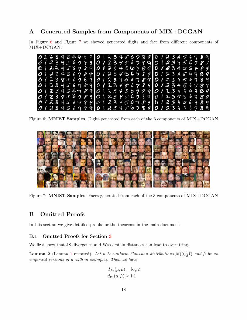
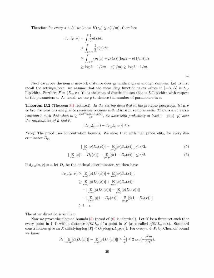
A Generated Samples from Components of MIX+DCGAN

In Figure 6 and Figure 7 we showed generated digits and face from different components ofMIX+DCGAN.

Figure 6: MNIST Samples. Digits generated from each of the 3 components of MIX+DCGAN

Figure 7: MNIST Samples. Faces generated from each of the 3 components of MIX+DCGAN

B Omitted Proofs

In this section we give detailed proofs for the theorems in the main document.

B.1 Omitted Proofs for Section 3

We first show that JS divergence and Wasserstein distances can lead to overfitting.

Lemma 2 (Lemma 1 restated). Let µ be uniform Gaussian distributions N (0, 1dI) and µ be an

empirical versions of µ with m examples. Then we have

dJS(µ, µ) = log 2

dW (µ, µ) ≥ 1.1

18

Proof. For Jensen-Shannon divergence, observe that µ is a continuous distribution and µ is discrete,therefore dJS(µ, µ) = log 2.

For Wasserstein distance, let x1, x2, ..., xm be the empirical samples (fixed arbitrarily). Fory ∼ N (0, 1

dI), by standard concentration and union bounds, we have

Pr[∀i ∈ [m]‖y − xi‖ ≥ 1.2] ≥ 1−m exp(−Ω(d)) ≥ 1− o(1).

Therefore, using the earth-mover interpretation of Wasserstein distance, we know dW (µ, µ) ≥1.2 Pr[∀i ∈ [m]‖y − xi‖ ≥ 1.2] ≥ 1.1.

Next we consider sampling for both the generated distribution and the real distribution, andshow that the JS divergence or Wasserstein distance do not generalize.

Theorem B.1. Let µ, ν be uniform Gaussian distributions N (0, 1dI). Suppose µ, ν are empirical

versions of µ, ν with m samples. Then with probability at least 1−m2 exp(−Ω(d)) we have

dJS(µ, ν) = 0,dJS(µ, ν) = log 2.

dW (µ, ν) = 0,dW (µ, ν) ≥ 1.1.

Further, let µ, ν be the convolution of µ, ν with a Gaussian distribution N(0, σ2

d I), as long asσ < c√

logmfor small enough constant c, we have with probability at least 1−m2 exp(−Ω(d)).

dJS(µ, ν) > log 2− 1/m.

Proof. For the Jensen-Shannon divergence, we know with probability 1 the supports of µ, ν aredisjoint, therefore dJS(µ, ν) = 1.

For Wasserstein distance, note that for two random Gaussian vectors x, y ∼ N(0, 1dI), their

difference is also a Gaussian with expected square norm 2. Therefore we have

Pr[‖x− y‖2 ≤ 2− ε] ≤ exp(−Ω(ε2d)).

As a result, setting ε to be a fixed constant (0.1 suffices), with probability 1−m2 exp(−Ω(d)),we can union bound over all the m2 pairwise distances for points in support of µ and support ofν. With high probability, the closest pair between µ and ν has distance at least 1, therefore theWasserstein distance dW (µ, ν) ≥ 1.1.

Finally we prove that even if we add noise to the two distributions, the JS divergence is stilllarge. For distributions µ, ν, let ρ1, ρ2 be their density functions. Let g(x) = ρ1(x) log 2ρ1(x)

ρ1(x)+ρ2(x) +

ρ2(x) log 2ρ2(x)ρ1(x)+ρ2(x) , we can rewrite the JS divergence as

dJS(µ, ν) =

∫1

2g(x)dx.

Let zx be a Bernoulli variable with probability ρ1(x)/(ρ1(x) + ρ2(x)) of being 1. Note that g(x) =(ρ1(x) + ρ2(x))(log 2 − H(zx)) where H(zx) is the entropy of zx. Therefore 0 ≤ g(x) ≤ (ρ1(x) +ρ2(x)) log 2. Let X be the union of radius-0.2 balls near the 2m samples in µ and ν. Since withhigh probability, all these samples have pairwise distance at least 1, by Gaussian density functionwe know (a) the balls do not intersect; (b) within each ball maxd1(x),d2(x)

mind1(x),d2(x) ≥ m2; (c) the union of

these balls take at least 1− 1/2m fraction of the density in (µ+ ν)/2.

19

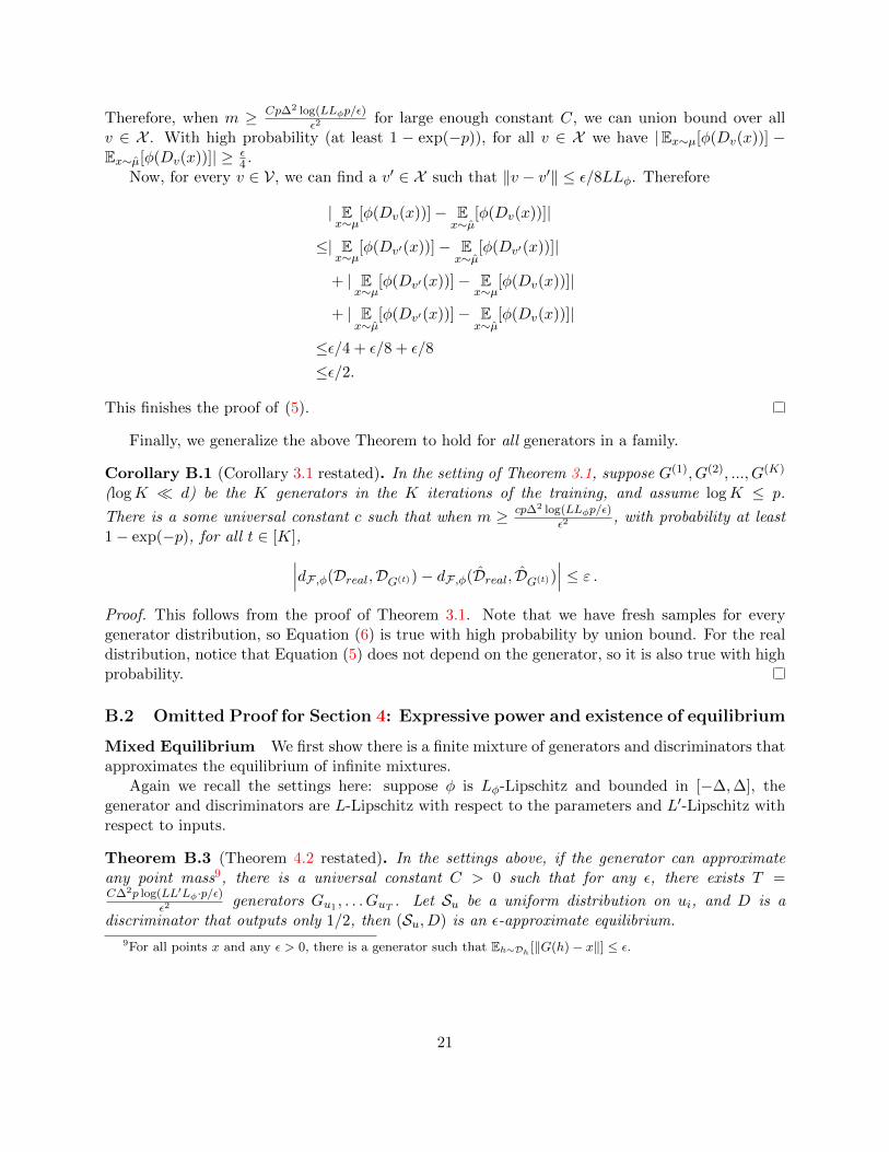
Therefore for every x ∈ X , we know H(zx) ≤ o(1/m), therefore

dJS(µ, ν) =

∫1

2g(x)dx

≥∫x∈X

1

2g(x)dx

≥∫x∈X

(ρ1(x) + ρ2(x))(log 2− o(1/m))dx

≥ log 2− 1/2m− o(1/m) ≥ log 2− 1/m.

Next we prove the neural network distance does generalize, given enough samples. Let us firstrecall the settings here: we assume that the measuring function takes values in [−∆,∆] is Lφ-Lipschitz. Further, F = Dv, v ∈ V is the class of discriminators that is L-Lipschitz with respectto the parameters v. As usual, we use p to denote the number of parameters in v.

Theorem B.2 (Theorem 3.1 restated). In the setting described in the previous paragraph, let µ, νbe two distributions and µ, ν be empirical versions with at least m samples each. There is a universal

constant c such that when m ≥ cp∆2 log(LLφp/ε)

ε2, we have with probability at least 1 − exp(−p) over

the randomness of µ and ν,|dF ,φ(µ, ν)− dF ,φ(µ, ν)| ≤ ε.

Proof. The proof uses concentration bounds. We show that with high probability, for every dis-criminator Dv,

| Ex∼µ

[φ(Dv(x))]− Ex∼µ

[φ(Dv(x))]| ≤ ε/2, (5)

| Ex∼ν

[φ(1−Dv(x))]− Ex∼ν

[φ(1−Dv(x))]| ≤ ε/2. (6)

If dF ,φ(µ, ν) = t, let Dv be the optimal discriminator, we then have

dF ,φ(µ, ν) ≥ Ex∼µ

[φ(Dv(x))] + Ex∼ν

[φ(Dv(x))].

≥ Ex∼µ

[φ(Dv(x))] + Ex∼ν

[φ(Dv(x))]

− | Ex∼µ

[φ(Dv(x))]− Ex∼µ

[φ(Dv(x))]|

− | Ex∼ν

[φ(1−Dv(x))]− Ex∼ν

[φ(1−Dv(x))]|

≥ t− ε.

The other direction is similar.Now we prove the claimed bounds (5) (proof of (6) is identical). Let X be a finite set such that

every point in V is within distance ε/8LLφ of a point in X (a so-called ε/8LLφ-net). Standardconstructions give an X satisfying log |X | ≤ O(p log(LLφp/ε)). For every v ∈ X , by Chernoff boundwe know

Pr[| Ex∼µ

[φ(Dv(x))]− Ex∼µ

[φ(Dv(x))]| ≥ ε

4] ≤ 2 exp(− ε

2m

2∆2).

20

Therefore, when m ≥ Cp∆2 log(LLφp/ε)

ε2for large enough constant C, we can union bound over all

v ∈ X . With high probability (at least 1 − exp(−p)), for all v ∈ X we have |Ex∼µ[φ(Dv(x))] −Ex∼µ[φ(Dv(x))]| ≥ ε

4 .Now, for every v ∈ V, we can find a v′ ∈ X such that ‖v − v′‖ ≤ ε/8LLφ. Therefore

| Ex∼µ

[φ(Dv(x))]− Ex∼µ

[φ(Dv(x))]|

≤| Ex∼µ

[φ(Dv′(x))]− Ex∼µ

[φ(Dv′(x))]|

+ | Ex∼µ

[φ(Dv′(x))]− Ex∼µ

[φ(Dv(x))]|

+ | Ex∼µ

[φ(Dv′(x))]− Ex∼µ

[φ(Dv(x))]|

≤ε/4 + ε/8 + ε/8

≤ε/2.

This finishes the proof of (5).

Finally, we generalize the above Theorem to hold for all generators in a family.

Corollary B.1 (Corollary 3.1 restated). In the setting of Theorem 3.1, suppose G(1), G(2), ..., G(K)

(logK d) be the K generators in the K iterations of the training, and assume logK ≤ p.

There is a some universal constant c such that when m ≥ cp∆2 log(LLφp/ε)

ε2, with probability at least

1− exp(−p), for all t ∈ [K],∣∣∣dF ,φ(Dreal,DG(t))− dF ,φ(Dreal, DG(t))∣∣∣ ≤ ε .

Proof. This follows from the proof of Theorem 3.1. Note that we have fresh samples for everygenerator distribution, so Equation (6) is true with high probability by union bound. For the realdistribution, notice that Equation (5) does not depend on the generator, so it is also true with highprobability.

B.2 Omitted Proof for Section 4: Expressive power and existence of equilibrium

Mixed Equilibrium We first show there is a finite mixture of generators and discriminators thatapproximates the equilibrium of infinite mixtures.

Again we recall the settings here: suppose φ is Lφ-Lipschitz and bounded in [−∆,∆], thegenerator and discriminators are L-Lipschitz with respect to the parameters and L′-Lipschitz withrespect to inputs.

Theorem B.3 (Theorem 4.2 restated). In the settings above, if the generator can approximateany point mass9, there is a universal constant C > 0 such that for any ε, there exists T =C∆2p log(LL′Lφ·p/ε)

ε2generators Gu1 , . . . GuT . Let Su be a uniform distribution on ui, and D is a

discriminator that outputs only 1/2, then (Su, D) is an ε-approximate equilibrium.

9For all points x and any ε > 0, there is a generator such that Eh∼Dh [‖G(h)− x‖] ≤ ε.

21

Proof. We first prove the value V of the game must be equal to 1/2.For the discriminator, onestrategy is to just output 1/2. This strategy has payoff 2φ(1/2) no matter what the generator does,so V ≥ 2φ(1/2).

For the generator, we use the assumption that for any point x and any ε > 0, there is a generator(which we denote by Gx,ε) such that Eh∼Dh [‖Gx,ε(h) − x‖] ≤ ε. Now for any ζ > 0, consider thefollowing mixture of generators: sample x ∼ Dreal, then use the generator Dx,ζ . Let Dζ be thedistribution generated by this mixture of generators. The Wasserstein distance between Dζ andDreal is bounded by ζ. Since the discriminator is L′-Lipschitz, it cannot distinguish between Dζand Dreal. In particular we know for any discriminator Dv

| Ex∼Dζ

[φ(1−Dv(x))]− Ex∼Dreal

[φ(1−Dv(x))]| ≤ O(LφL′ζ).

Therefore,

maxv∈V

Ex∼Dreal

[φ(Dv(x))] + Ex∼Dζ

[φ(1−Dv(x))]

≤O(LφL′ζ) + max

v∈VE

x∼Dreal[φ(Dv(x)) + φ(1−Dv(x))]

≤2φ(1/2) +O(LφL′ζ).

Here the last step uses the assumption that φ is concave. Therefore the value is upperbounded byV ≤ 2φ(1/2) +O(LφL

′ζ) for any ζ. Taking limit of ζ to 0, we have V = 2φ(1/2).The value of the game is 2φ(1/2) in particular means the optimal discriminator cannot do

anything other than a random guess. Therefore we will use a discriminator that outputs constant1/2. Next we will construct the generator.

Let (S ′u,S ′v) be the pair of optimal mixed strategies as in Theorem 4.1 and V be the optimalvalue. We will show that randomly sampling T generators from S ′u gives the desired mixture withhigh probability.

Construct ε/4LL′Lφ-nets V for the parameters of the discriminator V. By standard construc-tion, the sizes of these ε-nets satisfy log(|V |) ≤ C ′n log(LL′Lφ · p/ε) for some constant C ′. Letu1, u2, ..., uT be independent samples from S ′u. By Chernoff bound, for any v ∈ V , we know

Pr[ Ei∈[T ]

[F (ui, v)] ≥ Eu∈V

[F (u, v)] + ε/2] ≤ exp(− ε2T

2∆2).

When T =C∆2p log(L·Lφ·p/ε)

ε2and the constant C is large enough (C ≥ 2C ′), with high probability

this inequality is true for all v ∈ V . Now, for any v ∈ V, let v′ be the closest point in the ε-net. Bythe construction of the net, ‖v−v′‖ ≤ ε/4LL′Lφ. It is easy to check that F (u, v) is 2LL′Lφ-Lipschitzin both u and v, therefore

Ei∈[T ]

[F (ui, v′)] ≤ E

i∈[T ][F (ui, v)] + ε/2.

Combining the two inequalities we know for any v′ ∈ V,

Ei∈[T ]

[F (ui, v′)] ≤ 2φ(1/2) + ε.

This means the mixture of generators can win against any discriminator. By probabilisticargument we know there must exist such generators. The discriminator (constant 1/2) obviouslyachieve value V no matter what the generator is. Therefore we get an approximate equilibrium.

22

Pure equilibrium Now we show how to construct a larger generator network that gives a pureequilibrium.

Theorem B.4 (Theorem 4.3 restated). Suppose the generator and discriminator are both k-layerneural networks (k ≥ 2) with p parameters, and the last layer uses ReLU activation function. In thesetting of Theorem 4.2, there exists k+ 1-layer neural networks of generators G and discriminator

D with O(

∆2p2 log(LL′Lφ·p/ε)ε2

)parameters, such that there exists an ε-approximate pure equilibrium

with value 2φ(1/2).

In order to prove this theorem, the major step is to construct a generator that works as a mixtureof generators. More concretely, we need to construct a single neural network that approximatelygenerates the mixture distribution using the gaussian input it has. To do that, we can pass theinput h through all the generators Gu1 , Gu2 , ..., GuT . We then show how to implement a “multi-wayselector” that will select a uniformly random output from Gui(h) (i ∈ [T ]).

We first observe that it is possible to compute a step function using a two layer neural network.This is fairly standard for many activation functions.

Lemma 3. Fix an arbitrary q ∈ N and z1 < z2 < · · · < zq. For any 0 < δ < minzi+1 − zi, thereis a two-layer neural network with a single input h ∈ R that outputs q + 1 numbers x1, x2, ..., xq+1

such that (i)∑q+1

i=1 xi = 1 for all h; (ii) when h ∈ [zi−1 + δ/2, zi − δ/2], xi = 1 and all other xj’sare 010.

Proof. Using a two layer neural network, we can compute the function fi(h) = maxh−zi−δ/2δ , 0−maxh−zi+δ/2δ , 0. This function is 0 for all h < zi − δ/2, 1 for all h ≥ zi + δ/2 and changelinearly in between. Now we can write x1 = 1 − f1(h), xq+1 = fq(h), and for all i = 2, 3, ..., q,xq = fi(h)− fi−1(h). It is not hard to see that these functions satisfy our requirements.

Using these step functions, we can essentially select one output from the T generators.

Lemma 4. In the setting of Theorem 4.3, for any δ > 0, there is a k+ 1-layer neural network with

O(

∆2p2 log(LL′Lφ·p/ε)ε2

)parameters that can generate a distribution that is within δ total variational

difference with the mixture of Gu1 , Gu2 , ..., GuT .

The idea is simple: since we have implemented step functions from Lemma 3, we can just passthrough the input through all the generators Gu1 , ..., GuT . For the last layer of Gui , we add alarge multiple of −(1 − xi) where xi is the i-th output from the network in Lemma 3. Clearly, ifxi = 0 this is going to effectively disable the neural network; if xi = 1 this will have no effect. Byproperties of xi’s we know most of the time only one xi = 1, hence only one generator is selected.

Proof. Suppose the input for the generator is (h0, h) ∼ N(0, 1) × Dh (i.e. h0 is sampled from aGaussian, h is sampled according to Dh independently). We pass the input h through the generatorsand gets outputs Gui(h), then we use h0 to select one as the true output.

Let z1, z2, ..., zT−1 be real numbers that divides the probability density of a Gaussian into Tequal parts. Pick δ′ = δ/100T in Lemma 3, we know there is a 2-layer neural network that computesstep functions x1, ..., xT . Moreover, the probability that (x1, ..., xT ) has more than 1 nonzero entryis smaller than δ. Now, for the output of Gui(h), in each output ReLU gate, we add a very large

10When h ≤ z1 − δ/2 only x1 is 1 and when h ≥ zq + δ/2 only xq+1 = 1

23

multiple of −(1 − xi) (larger than the maximum possible output). This essentially “disables” theoutput when xi = 0 because before the result before ReLU is always negative. On the other hand,when xi = 1 this preserves the output. Call the modified network Gui , we know Gui = Gui whenxi = 1 and Gui = 0 when xi = 0. Finally we add a layer that outputs the sum of Gui . Byconstruction we know when (x1, ..., xT ) has only one nonzero entry, the network correctly outputsthe corresponding Gui(xi). The probability that this happens is at least 1−δ so the total variationaldistance with the mixture is bounded by δ.

Using the generator we constructed, it is not hard to prove Theorem 4.3. The only thing tonotice here is that when the generator is within δ total variational distance to the true mixture,the payoff F (u, v) can change by at most 2∆δ.

Proof of Theorem 4.3. Let T be large enough so that there exists an ε/2-approximate mixed equi-librium. Let the new set of generators be constructed as in Lemma 4 with δ ≤ ε/4∆ and Gu1 , ..., GuTfrom the original set of generators. Let D be the discriminator that always outputs 1/2,and G bethe generator constructed by the T generators from the approximate mixed equilibrium. DefineF ?(G,D) be the payoff of the new two-player game. Now, for any discriminator Dv, we have

F ?(G, v) ≤ Ei∈[T ]

F (ui, v) + |F ?(G,D′)− Ei∈[T ]

F (ui, v)|

≤ V + ε/2 + 2∆ε

4∆≤ V + ε.

The bound from the first term comes from Theorem 4.2, and the fact that the expectation is smallerthan the max. The bound for the second term comes from the fact that changing a δ fraction ofprobability mass can change the payoff F by at most 2∆δ. Therefore the generator can still foolall discriminators, and we get a pure equilibrium.

C Examples when best response fail

In this section we construct simple generators and discriminators and show that if both generatorsand discriminators are trained to optimal with respect to Equation (2), the solution will cycle andcannot converge. For simplicity, we will show this when the connection function is φ, but it ispossible to show similar result even when φ is the traditional log function.

We consider a simple example where we try to generate points on a circle. The true distributionDtrue has 1/3 probability to generate a point at angle 0, 2π/3, 4π/3. Let us first consider a casewhen the generator does not have enough capacity to generate the true distribution.

Definition 4 (Example 1). The generator G has one parameter θ ∈ [0, 2π), and always generates apoint at angle θ. The discriminator D has a parameter φ ∈ [0, 2π), and Dφ(τ) = exp(−10d(τ, φ)2).Here d(τ, φ) is the angle between τ and φ and is always between [0, π].

We will analyze the “best response” procedure (as in Algorithm 1). We say the procedureconverges if limi→∞ φ

i and limi→∞ θi exist.

24

Algorithm 1 Best Response

Initialize θ0.for i = 1 to T do

Let φi = arg maxφ Eτ∼Dtrue [Dφ(τ)]− Eτ∼G(θ)[Dφ(τ)].Let θi = arg minθ −Eτ∼G(θ)[Dφ(τ)].

end for

Theorem C.1. For generator G and discriminator D in Example 1, for every choice of parameterθ, there is a choice of φ such that Dφ(θ) ≤ 0.001 and Eτ∼Dt∇ue [Dφ(τ)] ≥ 1/3. On the other hand,for every choice of φ, there is always a θ such that Dφ(θ) = 1. As a result, the sequence of bestresponse cannot converge.

Proof. For any θ, we can just choose φ to be the farthest point in 0, 2π/3, 4π/3. Clearly thedistance is at least 2π/3 and therefore Dφ(θ) ≤ exp(−10) ≤ 0.001. On the other hand, for the truedistribution, it has 1/3 probability of generating the point φ, therefore Eτ∼Dt∇ue [Dφ(τ)] ≥ 1/3.For every φ, we can always choose θ = φ, and we have Dφ(θ) = 1.

By the construction of φi and θi in Algorithm 1, we know for any i Dφi(θi) = 1, but Eτ∼Dtrue [Dφ(τ)]−

Dφi−1(θi) ≥ 1/4. Therefore |Dφi(θi) − Dφi−1(θi)| ≥ 1/4 for all i and the sequences cannot con-

verge.

This may not be very surprising as the generator does not even have the capacity to generate thetrue distribution. One might hope that once we use a large enough neural network, the generatorwill be able to generate the true distribution. However, our next example shows even in that casethe best response algorithm may not converge.

Definition 5 (Example 2). Let θ, φ ∈ [0, 2π)3 will be 3 -dimensional vectors. The generator G(θ)generates the uniform distribution over points θ1, θ2, θ3. The discriminator function is chosen to beDφ(τ) = 1

3

∑3i=1 exp(−10d(τ, φi)

2).

Clearly in this example, the true distribution can be generated by the generator (just by choosingθ = (0, 2π/3, 4π/3)). However we will show that the best response algorithm still cannot alwaysconverge.

Theorem C.2. Suppose the generator and discriminator are described as in Example 2, and θ0 =(0, 0, 0), then we have: (1) In every iteration the three points for generator θi1,2,3 are equal to each

other. (2) In every iteration θi1 is 0.1-close to one of the true points 0, 2π/3, 4π/3, and its closestpoint is different from the previous iteration.

Before giving detailed calculations, we first give an intuitive argument. In this example, wewill use induction to prove that at every iteration t, two properties are preserved: 1. The threepoints of the generator (θt1, θ

t2, θ

t3) are close to the same real example (0, 2π/3 or 4π/3); 2. The

three points of the discriminator (φt+11 , φt+1

2 , φt+13 ) will be close to the other two real examples. To

go from 1 to 2, notice that in this case the three φ values can be optimized independently (andthe final objective is the sum of the three), so it suffices to argue for one of them. For one φ, byour construction the objective function is really close to the sum of two Gaussians at the other tworeal examples, minus twice of a Gaussian at the real example that θti ’s are close to (see Figure 8).From the Figure it is clear that the maximum of this function is close to one of the real examples

25

Figure 8: Optimization problem for φ

that is different from θti .Now all the three φt+1i ’s will be close to one of the two real examples, so

one of them is going to get at least two φt+1i ’s. In the next iteration, as the generator is trying

to maximize the output of discriminator, all three θt+1i ’s will be close to the real example with at

least two φt+1i ’s.

Now we make this intuition formal through calculations.

Proof. The optimization problems here are fairly simple and we can argue about the solutionsdirectly. Throughout the proof we will use the fact that exp(−10∗(2π/3)2) < 1e−4 and exp(1+ε) ≈1 + ε. The following claim describes the properties we need:

Claim 1. If θ1 = θ2 = θ3 and θ1 is 0.1-close to one of 0, 2π/3, 4π/3, then the optimal φ mustsatisfy φ1, φ2, φ3 be 0.05-close to the other two points in 0, 2π/3, 4π/3.

We first prove the Theorem with the claim. We will do this by induction. The inductionhypothesis is that for every j ≤ t, we have θj1,2,3 are equal to each other, and θj1 is 0.1-close to oneof the true points 0, 2π/3, 4π/3. This is clearly true for t = 0. Now let us assume this is true fort and consider iteration t+ 1.

Without loss of generality we assume θt1 is close to 0. Now by Claim we know φt1, φt2, φ

t3 are

0.05-close to either 2π/3 or 4π/3. Without loss of generality assume there are more φti’s closeto 2π/3 (the number of φti’s close to the two point has to be different because there are 3 φti’s).Now, by property of Gaussians, we know Dφt(τ) has a unique maximum that is within 0.1 of 2π/3(the influence from the other point is much smaller than 0.05). Since the generator is trying tomaximize Eτ∼G(θ)[Dφ(τ)], all three θti(i = 1, 2, 3) should be at this maximizer. This finishes theinduction.

Now we prove the claim.

Proof. The objective function is

maxφ

1

3

(E

τ∼Dtrue[

3∑i=1

exp(−10d(τ, φi)2)]− E

τ∼G(θ)[

3∑i=1

exp(−10d(τ, φi)2)]

).

26

In this objective function φi’s do not interact with each other, so we can break the objective functioninto three (one for each φi). Without loss of generality, assume θ1,2,3 are 0.1-close to 0, we are tryingto maximize

maxφ

(1

3

3∑i=1

exp(−10d(φ, i · 2π/3)2)]− exp(−10d(θ, φ)2)

).

Clearly, if φ is not 0.05 close to either 2π/3 or 4π/3, we have D ≤ 1/3− 10 · 0.052 + exp(−10) ≤1/3− 0.02. On the other hand, when φ = 2π/3 or 4π/3, we have D ≥ 1/3− exp(−10). Thereforethe maximum must be 0.05-close to one of the two points.

Note that this example is very similar to the mode collapse problem mentioned in NIPS 2016GAN tutorial[Goodfellow, 2016].

27