Generalisations of Pick’s Theorem to Reproducing Kernel Hilbert...
120
Generalisations of Pick’s Theorem to Reproducing Kernel Hilbert Spaces Ph.D. Thesis submitted to Lancaster University by Peter Philip Quiggin M.A. Department of Mathematics and Statistics Lancaster University, United Kingdom August 1994
Transcript of Generalisations of Pick’s Theorem to Reproducing Kernel Hilbert...

Generalisations of Pick’s Theorem to ReproducingKernel Hilbert Spaces
Ph.D. Thesis submitted to Lancaster Universityby Peter Philip Quiggin M.A.
Department of Mathematics and StatisticsLancaster University, United Kingdom
August 1994

Contents
Abstract 3
Acknowledgments 4
Introduction and Overview 5
1 The Scalar-Valued Case 8
1.1 Reproducing Kernel Hilbert Spaces . . . . . . . . . . . . . . . . . . 8
1.2 Generalising Pick’s Theorem . . . . . . . . . . . . . . . . . . . . . . 10
1.3 One-Point Extensions Are Sufficient . . . . . . . . . . . . . . . . . . 13
1.4 Minimal Norm Extension . . . . . . . . . . . . . . . . . . . . . . . . 17
1.5 Sufficient Conditions for Pick’s Theorem . . . . . . . . . . . . . . . 26
2 Scalar-Valued Applications 30
2.1 Weighted Hardy Spaces . . . . . . . . . . . . . . . . . . . . . . . . . 30
2.2 Weighted Sobolev Spaces . . . . . . . . . . . . . . . . . . . . . . . . 32
2.3 Other Cases . . . . . . . . . . . . . . . . . . . . . . . . . . . . . . . 35
3 Uniqueness of the Optimal Interpolant 39
3.1 Uniqueness for One Point Extension . . . . . . . . . . . . . . . . . . 40
3.2 Blaschke Kernels . . . . . . . . . . . . . . . . . . . . . . . . . . . . 47
4 The Operator-Valued Case 52
4.1 Vector-Valued Reproducing Kernel Spaces . . . . . . . . . . . . . . 53
4.2 Generalising the Operator Pick Theorem . . . . . . . . . . . . . . . 57
1

4.3 One-Point Extensions Are Sufficient . . . . . . . . . . . . . . . . . . 58
4.4 Minimal Norm Extension . . . . . . . . . . . . . . . . . . . . . . . . 59
4.5 Sufficient Conditions for Pick’s Theorem . . . . . . . . . . . . . . . 62
5 Completely NP Kernels 66
5.1 Characterisation of 3 by 3 NP Kernels . . . . . . . . . . . . . . . . 67
5.2 Characterisation of Completely NP kernels . . . . . . . . . . . . . . 70
5.3 An NP kernel that is not Completely NP . . . . . . . . . . . . . . . 81
6 Generalised Kernels 85
6.1 Schwartz Kernels . . . . . . . . . . . . . . . . . . . . . . . . . . . . 86
6.2 Reproducing Kernel Kreın Spaces . . . . . . . . . . . . . . . . . . . 89
6.3 Relationship to Aronszajn’s Kernels . . . . . . . . . . . . . . . . . . 90
6.4 Negativity of Kernel Differences . . . . . . . . . . . . . . . . . . . . 91
7 The Adamyan-Arov-Kreın Theorem 96
7.1 Introduction . . . . . . . . . . . . . . . . . . . . . . . . . . . . . . . 96
7.2 Kernel Characterisation of sk . . . . . . . . . . . . . . . . . . . . . 99
7.3 sk for Functions on the Disc . . . . . . . . . . . . . . . . . . . . . . 102
7.4 One Point Extension . . . . . . . . . . . . . . . . . . . . . . . . . . 105
7.5 Proof of the AAK Theorem . . . . . . . . . . . . . . . . . . . . . . 109
Conclusions 113
Nomenclature 115
Bibliography 116
2

Generalisations of Pick’s Theorem
to Reproducing Kernel Hilbert Spaces
Ph.D. Thesis submitted to Lancaster University
by Peter Philip Quiggin M.A.
Department of Mathematics and Statistics
Lancaster University, United Kingdom.
August 1994
Abstract
Pick’s theorem states that there exists a function in H∞, which is bounded by 1
and takes given values at given points, if and only if a certain matrix is positive.
H∞ is the space of multipliers of H2 and this theorem has a natural generalisation
when H∞ is replaced by the space of multipliers of a general reproducing kernel
Hilbert space H(K) (where K is the reproducing kernel). J. Agler showed that this
generalised theorem is true when H(K) is a certain Sobolev space or the Dirichlet
space. This thesis widens Agler’s approach to cover reproducing kernel Hilbert
spaces in general and derives sufficient (and usable) conditions on the kernel K,
for the generalised Pick’s theorem to be true for H(K). These conditions are
then used to prove Pick’s theorem for certain weighted Hardy and Sobolev spaces
and for a functional Hilbert space introduced by Saitoh. The reproducing kernel
approach is then used to derived results for several related problems. These include
the uniqueness of the optimal interpolating multiplier, the case of operator-valued
functions and a proof of the Adamyan-Arov-Kreın theorem.
MSC 1991 : Primary 30E05
Secondary 46E22, 47A20.
3

Acknowledgments
This research draws heavily on ideas developed by Prof. J. Agler in an (as yet)
unpublished draft paper in which he proves Pick’s theorem for the Dirichlet space.
The overall approach stems from Agler’s work, and in particular lemma 1.4.2 and
the main idea for the proof of lemma 1.3.3 are derived from that paper. I would
like to thank Prof. Agler for the stimulus his ideas have given. I would also like
to thank Scott McCullough, who showed the way forward on the completely NP
kernels described in chapter 5.
Most importantly, however, I would like to thank my supervisor, Prof. N. Young,
for many useful and enjoyable discussions, much inspiration and several key ideas,
in particular for the proofs of lemma 1.4.3 and theorem 2.2.3.
This work was supported by a grant from the Science and Engineering Research
Council, for which I am very grateful.
Declaration
The contents of chapters 1 and 2 of this thesis have previously been published as
a paper in the journal Integral Equations and Operator Theory [Qui93].
4

Introduction and Overview
Pick’s theorem is a result about interpolation for complex-valued functions. Sup-
pose we are asked to find an analytic function φ : D→ C on the unit disk D whose
supremum norm ‖φ‖∞ = supz∈D |φ(z)| is as small as possible and yet φ satisfies the
interpolation requirement that φ(xi) = zi (i = 1, . . . , n). Here x1, . . . , xn ∈ D are
some given points and z1, . . . , zn ∈ C are given values that the function must take
at those points. Pick’s theorem addresses the question: how small can we make
‖φ‖∞ and yet still satisfy the interpolation requirement? It states:
There exists an analytic function φ : D → C for which ‖φ‖∞ ≤ 1 and
φ(xi) = zi (i = 1, . . . , n) if and only if the matrix
(1− ziz∗j1− xix∗j
)i,j=1,...,n
is positive.
Because scaling the data values zi simply scales the possible solutions φ and their
norms ‖φ‖∞, this result effectively answers our question. For
there exists φ such that ‖φ‖∞ ≤ r and φ(xi) = zi
⇔ there exists φ such that ‖φ‖∞ ≤ 1 and φ(xi) = zi/r
⇔(
1− ziz∗j /r2
1− xix∗j
)i,j=1,...,n
is positive
⇔(r2 − ziz∗j1− xix∗j
)i,j=1,...,n
is positive
5

so the best we can achieve for ‖φ‖∞ is
infr≥0
r :
(r2 − ziz∗j1− xix∗j
)i,j=1,...,n
is positive
.
Pick proved his theorem in 1916 [Pic16] using function-theoretic methods, but
because of its importance it continued to be studied by many authors and in 1967
Donald Sarason [Sar67] gave a radically new, and particularly natural, operator-
theoretic interpretation and proof of the result. In Sarason’s approach the function
φ is represented by the operator on the Hardy space H2 of multiplication by φ, the
norm ‖φ‖∞ equals the norm of this operator and Pick’s theorem is then a result
about multiplication operators on H2. This is one example of an interplay between
function theory and operator theory that has proved fruitful in recent decades—
some aspects of Pick’s theorem are easier to understand from the operator-theoretic
viewpoint, whereas others are easier from a function-theoretic viewpoint.
H2 is a reproducing kernel Hilbert space, i.e. it is a Hilbert space of complex-
valued functions on some set X (= D in this case) in which all of the point-
evaluation functionals f 7→ f(x), x ∈ X, are continuous. Each such space has a
unique associated function K : X × X → C, called its reproducing kernel, which
completely characterises the space and can be used to study it. I denote the space
corresponding to kernel K by H(K).
In the late 1980s, J. Agler shone further light on Pick’s theorem using H2’s repro-
ducing kernel. He showed that the operator-theoretic form of Pick’s theorem still
holds if H2 is replaced by certain other reproducing kernel Hilbert spaces. The
research in this thesis began when I read an early draft paper by Agler in which
he proved this variation of Pick’s theorem for the Dirichlet space. It appeared
that Agler’s approach could be generalised to any reproducing kernel Hilbert space
whose kernel satisfied suitable properties and this lead me to ask the question ‘For
which reproducing kernel Hilbert spaces is Pick’s theorem true?’. Chapters 1 and 2
6

are the result of this enquiry and are essentially as published in my paper [Qui93].
Chapter 1 derives sufficient conditions on the kernel K for Pick’s theorem to hold
for H(K) and chapter 2 applies this result to several specific cases.
The following two chapters examine whether the reproducing kernel approach can
also be used to prove and generalise some other results related to Pick’s theorem.
Chapter 3 studies the known fact that for H2 there is a unique analytic inter-
polating function that has the smallest possible norm ‖φ‖∞ and shows that this
uniqueness result also holds for a class of spaces closely related to H2. In chapter 4
the reproducing kernel approach is generalised to interpolation of operator-valued
functions.
The sufficient conditions derived in chapter 1 frustrated me. Numerous computer
calculations with randomly chosen kernels that failed to satisfy the condition all
found that the generalised Pick’s theorem also failed to hold with those kernels.
This lead me into a lengthy, but failed, attempt to prove that the conditions on
the kernel K are also necessary. Only later did it become apparent, from studying
related work by Scott McCullough [McC92], that this attempt was doomed to fail
since the conditions are not necessary—they in fact characterise a slightly stronger
property of the kernel. Chapter 5 describes this stronger property and derives an
explicit counter-example to necessity.
The final two chapters cover another very important derivative of Pick’s theorem—
the Adamyan-Arov-Kreın theorem. This difficult result, proved in 1971 [AAK71],
has important applications in control theory. Chapter 7 addresses the question ‘Can
the reproducing kernel approach shed light on the Adamyan-Arov-Kreın theorem
and perhaps even generalise it further?’. My attempts to answer this question
lead me to some much more general results about reproducing kernels, which are
described in chapter 6.
7
Chapter 1
The Scalar-Valued Case
This chapter studies Pick’s theorem for reproducing kernel Hilbert spaces of scalar-
valued functions.
1.1 Reproducing Kernel Hilbert Spaces
I will start by defining notation and stating the main facts which we will need from
the theory of reproducing kernel Hilbert spaces. For details and proofs of these
facts, see [Aro50] and [Sai88].
Given a set X, a kernel K on X is a complex-valued function on X × X. When
the set X is a finite set I will call K a finite kernel. Finite kernels can be viewed as
matrices; in fact kernels are effectively generalisations of matrices, and in line with
this analogy I will call the functions K(x, ·) and K(·, x) the x-row and x-column of
K, respectively. The restriction of K to the set E ×E, where E is any non-empty
subset of X, will be denoted KE, and kernel K is called positive or positive-definite,
denoted K ≥ 0 and K > 0, whenever its finite restrictions are all positive or all
positive-definite matrices, respectively.
Given any Hilbert space H of complex-valued functions on a set X, for which the
point-evaluation linear functionals are all continuous, it can be shown that there
8

exists a unique positive kernel K which has the following ‘reproducing’ property
for H:
for all f ∈ H and all x ∈ X, K(·, x) ∈ H and f(x) = 〈f,K(·, x)〉
where 〈·, ·〉 denotes the inner product in H.
Conversely, it is also true that to every positive kernel K on a set X there corre-
sponds a unique Hilbert space of complex-valued functions on X, for which K is
the reproducing kernel. I indicate this association between the positive kernel K
and the corresponding reproducing kernel Hilbert space by denoting the latter as
H(K). The space H(K) is easily described—it is the completion of the span of the
columns of K; i.e. the functions in H(K) are all limits of finite linear combinations
of the columns of K. And the inner product in H(K) is the extension to the whole
space of the inner product defined on the columns of K by
〈K(·, y), K(·, x)〉 = K(x, y).
The functions in H(K), and their norms, can also be characterised by a positivity
condition—they are exactly the functions f on X for which r2K − f ⊗ f ∗ ≥ 0 for
some real r ≥ 0 (where r2K − f ⊗ f ∗ denotes the kernel r2K(x, y) − f(x)f(y)∗).
The set of such r (for which r2K− f ⊗ f ∗ ≥ 0) is either empty if f is not in H(K),
or else is the half open interval [‖f‖,∞), where ‖f‖ is f ’s norm in H(K).
Given a positive kernel K, a function φ : X → C is called a multiplier of H(K) if
H(K) is closed under multiplication by φ. When this happens multiplication by φ
always turns out to be a bounded linear operator on H(K), which I denote by Mφ,
and the operator norm of Mφ gives a ‘multiplier’ norm for φ, denoted ‖φ‖M(K). I
will denote the space of multipliers of H(K), with this multiplier norm, by M(K).
The functions in M(K), and their multiplier norms, are again characterised by a
positivity condition—they are the functions φ on X for which (r2 − φ⊗ φ∗)K ≥ 0
9

for some non-negative r. The set of such r (for which (r2−φ⊗φ∗)K ≥ 0) is either
empty if φ is not in M(K), or else is the half open interval [‖φ‖M(K),∞).
If K is positive-definite, then when we restrict K to a subset E of X the resulting
spaces H(KE) and M(KE) relate to H(K) and M(K) in a simple way. Let H(K,E)
denote the closed subspace of H(K) spanned by the columns of K corresponding
to the subset E. Then the mapping
U : H(KE)→ H(K,E) KE(·, x) 7→ K(·, x) for all x ∈ E
is unitary, since the E columns of KE and of K have the same Gram matrix, namely
KE. Therefore U is a unitary embedding of H(KE) in H(K).
Given a function f : E → C that is in M(KE), its corresponding multiplication
operator Mf is an operator on H(KE). But U is effectively an identification of
H(KE) as H(K,E) and so allows us to work instead with the unitarily equivalent
operator UMfU−1 on H(K,E), which I will denote as Mf . We will sometimes
work with Mf rather than Mf , the advantage being that Mf is an operator on a
subspace of H(K).
If K is a positive kernel and φ ∈ M(K) is a multiplier of H(K), let φE be its
restriction to the subset E. Then from the above characterisation of multiplier
norms we have (‖φ‖2M(K) − φ ⊗ φ∗)K ≥ 0. But (‖φ‖2
M(K) − φE ⊗ φ∗E)KE is a
restriction of this kernel, and so must also be positive; so φE is a multiplier of
H(KE) and ‖φE‖M(KE) ≤ ‖φ‖M(K). In words, the restriction to E of a multiplier
of H(K) is a multiplier of H(KE) with equal or smaller norm.
1.2 Generalising Pick’s Theorem
Nevanlinna [Nev19] and Pick [Pic16] studied the problem of interpolation by bounded
analytic functions early this century, and much more recently Sarason [Sar67] set
their results in an operator-theoretic context.
10

Pick’s original theorem states:
There exists a function φ ∈ H∞, with ‖φ‖∞ ≤ 1, that takes the n given
data values zi ∈ C at the n given data points xi ∈ D if and only if(1− ziz∗j1− xix∗j
)i,j=1,...,n
≥ 0.
We can now set this into the context of reproducing kernel Hilbert spaces and the
notation defined above. Let
X = the open unit disc D
K = the Szego kernel K(x, y) = 1/(1− xy∗)
E = the set of data points {x1, . . . , xn}
KE = the restriction of K to E
and f = the function on E defined by f(xi) = zi.
Then H(K) = H2, M(K) = H∞, ‖ · ‖M(K) = ‖ · ‖∞, and the matrix in Pick’s
theorem is simply the finite kernel (1 − f ⊗ f ∗)KE, positivity of which is, from
above, equivalent to ‖f‖M(KE) ≤ 1. We can therefore restate Pick’s theorem as
(1) There exists a multiplier φ ∈M(K), with ‖φ‖M(K) ≤ 1, that is an
extension of the multiplier f ∈M(KE)
if and only if
(2) ‖f‖M(KE) ≤ 1.
It is now clear why (1) ⇒ (2); simply because f is then the restriction of φ to E
and so (see section 1.1) must have multiplier norm no greater than that of φ. So
the ‘meat’ of Pick’s theorem is the sufficiency of (2), i.e. that every multiplier of
H(KE) has an extension to a multiplier of H(K) with no greater (and therefore
equal) norm.
11

With this in mind I define the following terminology. If E and F are non-empty
subsets of X and F contains E, then I will say that all multipliers on E extend
isometrically to F if all multipliers in M(KE) have extensions in M(KF ) with equal
norm.
If multipliers on E extend isometrically to F , then they clearly also extend isomet-
rically to any subset F1 of F that contains E, since we can extend any multiplier
in M(KE) to F and then restrict back to F1, all without increasing the multiplier
norm.
It is clear from the above discussion that the following, which I will refer to as the
full Pick theorem, is true for H(K) if and only if all multipliers on all non-empty
subsets of X extend isometrically to X:
Given a function f on any non-empty subset E of X, there exists an
extension φ ∈ M(K) of f , with ‖φ‖M(K) ≤ 1 if and only if the kernel
(1− f ⊗ f ∗)KE is positive.
I will call the weakening that results if only finite subsets E are allowed, the finite
Pick theorem:
Given a function f on any finite non-empty subset E of X, there exists
an extension φ ∈M(K) of f , with ‖φ‖M(K) ≤ 1 if and only if the kernel
(1− f ⊗ f ∗)KE is positive.
Clearly it is true if and only if all multipliers on non-empty finite subsets of X
extend isometrically to X.
In this terminology, Pick’s original theorem is the finite Pick theorem for the
case where H(K) is the Hardy space H2. It is also known that the finite Pick
theorem is true for several other reproducing kernel Hilbert spaces, including a
12

Sobolev space on [0,1] (see [Agl90]), and the Dirichlet space on D [Agl88]. And
more restricted forms of Pick’s theorem, for example with conditions placed on the
subset E, have been proved for some classes of reproducing kernel Hilbert spaces
[Sai88] [BB84] [Sza86]. However neither the finite nor the full Pick theorem are
true for all reproducing kernel Hilbert spaces—Beatrous and Burbea [BB84] show
this, and in section 2.3 I give other examples.
The question that we would like to answer is: for which positive kernels K are
these two theorems true for H(K)? Hopefully it is now clear that this question
comes down to asking which extensions of multipliers can be done isometrically.
1.3 One-Point Extensions Are Sufficient
The property of being able to extend all multipliers isometrically, from one subset
E of X to a larger one F , is clearly transitive. I.e. if we can extend all multipliers
isometrically from E to F , and also from F to G, then we can do so from E to G.
Because of this, the extensions where exactly one extra point is added (i.e. from E
to E∪{t} where t ∈ X \E) are elementary extensions from which larger extensions
can be built, and I will call these one-point extensions. In this section I show it is
sufficient to know that all one-point extensions can be done isometrically.
Firstly, we will need the following characterisation of multiplication operators on
reproducing kernel Hilbert spaces.
Lemma 1.3.1 Given a positive kernel K on a set X, an operator M on H(K) is
a multiplication operator (i.e. M is the same as multiplication by some multiplier
in M(K)) if and only if every column of K is an eigenvector of M∗. Further, if M
is a multiplication operator then M∗’s eigenvalue corresponding to the y-column of
K is φ(y)∗ where φ is the corresponding multiplier.
13

Proof: ⇒ If M is the operator of multiplication by multiplier φ, then for all
y ∈ X
M∗(K(·, y))(x) = 〈M∗(K(·, y)), K(·, x)〉
= 〈K(·, y),M(K(·, x))〉
= 〈K(·, y), φ(·)K(·, x)〉
= 〈φ(·)K(·, x), K(·, y)〉∗
= φ(y)∗K(y, x)∗ = φ(y)∗K(x, y)
= (φ(y)∗K(·, y))(x).
Therefore K(·, y) is an eigenvector of M∗, with eigenvalue φ(y)∗.
⇐ Given an operator M such that all columns of K are eigenvectors of M∗,
define the function φ : X → C by φ(y)∗ = M∗’s eigenvalue corresponding
to the y-column of K. Then for all y ∈ X
M(K(·, y))(x) = 〈M(K(·, y)), K(·, x)〉
= 〈K(·, y),M∗(K(·, x))〉
= 〈K(·, y), φ(x)∗K(·, x)〉
= (φ(·)K(·, y))(x).
So M and multiplication by φ agree on all columns of K, and by linearity
they must also agree on the linear span of K’s columns. But for any
f ∈ H(K), f is the limit of some sequence of functions (fn)n∈N in the
linear span of K’s columns, so
M(f)(x) = lim(M(fn))(x)
= lim(M(fn)(x))
= lim(φ(x)fn(x))
= φ(x) lim(fn(x))
= φ(x)f(x)
14
Therefore M and multiplication by φ agree on the whole of H(K).
We can now prove that one-point isometric extensions are sufficient. Following
Agler, I will call a positive kernel for which all one-point extensions can be done
isometrically a Nevanlinna-Pick kernel, abbreviated for convenience to NP kernel.
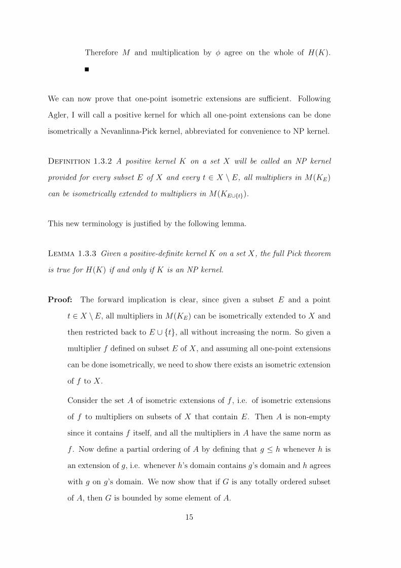
Definition 1.3.2 A positive kernel K on a set X will be called an NP kernel
provided for every subset E of X and every t ∈ X \ E, all multipliers in M(KE)
can be isometrically extended to multipliers in M(KE∪{t}).
This new terminology is justified by the following lemma.
Lemma 1.3.3 Given a positive-definite kernel K on a set X, the full Pick theorem
is true for H(K) if and only if K is an NP kernel.
Proof: The forward implication is clear, since given a subset E and a point
t ∈ X \E, all multipliers in M(KE) can be isometrically extended to X and
then restricted back to E ∪ {t}, all without increasing the norm. So given a
multiplier f defined on subset E of X, and assuming all one-point extensions
can be done isometrically, we need to show there exists an isometric extension
of f to X.
Consider the set A of isometric extensions of f , i.e. of isometric extensions
of f to multipliers on subsets of X that contain E. Then A is non-empty
since it contains f itself, and all the multipliers in A have the same norm as
f . Now define a partial ordering of A by defining that g ≤ h whenever h is
an extension of g, i.e. whenever h’s domain contains g’s domain and h agrees
with g on g’s domain. We now show that if G is any totally ordered subset
of A, then G is bounded by some element of A.
15

SubProof: For each g ∈ G let
Fg = domain of g
F = ∪g∈GFg
KFg = the restriction of K to Fg
Hg = H(KF , Fg), the closed subspace of H(KF ) spanned by the columns
of KF corresponding to Fg
Mg = the operator on Hg that corresponds to multiplication of H(KFg)
by g. Recall that H(KFg) embeds naturally as Hg in H(KF ), so
operators on H(KFg) induce unitarily equivalent operators on Hg.
Then the operators Mg all have norm ‖f‖M(KE), and their adjoints M∗g
form a ‘nest’ in the following sense. Let M∗g1
and M∗g2
be any two such
operators; since G is totally ordered we can assume (without loss of
generality) that g1 ≤ g2. Then Hg1 is a M∗g2
-invariant subspace of Hg2 ,
since it is generated by the Fg1-columns of K, which are all eigenvectors
of M∗g2
. And M∗g1
is simply M∗g2
restricted to Hg1 .
Now define the linear transformation M∗, on the union of the Hg’s, by
M∗(h) = M∗g (h) where g is any element of G such that h ∈ Hg. Because
we have a ‘nest’ of operators this is well-defined, and because each M∗g
has norm ‖f‖M(KE) then so does M∗.
We can now extend M∗ by continuity, without increasing its norm, to
an operator on the norm-closure of the union of the Hg’s in H(KF ),
which is the whole of H(KF ). This gives a well-defined operator M∗ on
H(KF ) whose restrictions to the subspaces Hg (which are M∗-invariant)
are the operators M∗g .
Since M∗g ’s eigenvectors include all the Fg-columns of KF for all g ∈ G,
all columns of KF are eigenvectors of M∗, so (by lemma 1.3.1) M is a
multiplication operator on H(KF ). Let the corresponding multiplier be
16

φ; then from the way M was constructed, φ is an extension of each g in
G, and has the same norm ‖f‖M(KE). Therefore φ is in A, and g ≤ φ
for all g ∈ G, so G is bounded in A, as required.
Since all totally ordered subsets of A are bounded (and assuming the Axiom
of Choice), A has a maximal element φ say, by Zorn’s lemma. But then
φ’s domain must be the whole of X, since otherwise (by assumption) there
would exist a one-point extension of φ which would be in A and greater than
φ, contradicting φ’s maximality. φ is therefore an isometric extension of f to
the whole of X, as required.
1.4 Minimal Norm Extension
Throughout this section, let X be any set, K be a positive-definite kernel on X, t
be any point of X, and E = X \ {t}. We will consider the problem of extending
a given multiplier f on E to a multiplier φ on X which has the smallest possible
norm. Agler [Agl88] has given an explicit formula for this smallest possible norm,
and shown that it is achievable. Here we will derive Agler’s result from Parrott’s
theorem, but first we need to move over to an operator-theoretic way of viewing
the problem. Initially, let us restrict attention to X being a finite set; at the end
of this section we will see that the main result also holds for infinite X.
Corresponding to the given multiplier f is its multiplication operator adjoint M∗f
on H(KE), which in turn induces an operator M∗f on H(K,E) (the closure of the
span of the E-columns, which is the subspace of H(K) corresponding to H(KE)).
M∗f is simply the operator that has the E-columns of K as its eigenvectors with
f(x)∗ as its eigenvalues; in other words it is a diagonal operator with respect to
the basis given by the E-columns of K. Because K is positive-definite and E is
finite, K(·, t) is not in H(K,E) so the process of one-point extending f to the
17
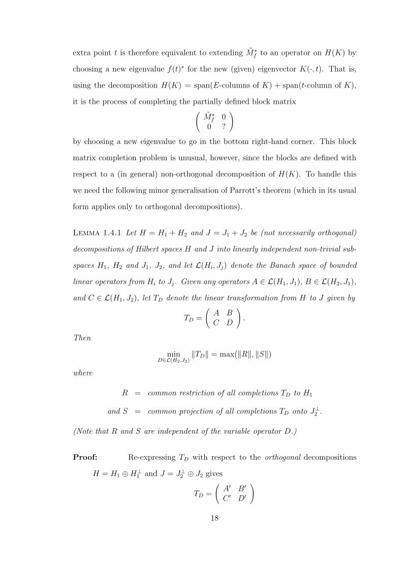
extra point t is therefore equivalent to extending M∗f to an operator on H(K) by
choosing a new eigenvalue f(t)∗ for the new (given) eigenvector K(·, t). That is,
using the decomposition H(K) = span(E-columns of K) + span(t-column of K),
it is the process of completing the partially defined block matrix(M∗
f 00 ?
)
by choosing a new eigenvalue to go in the bottom right-hand corner. This block
matrix completion problem is unusual, however, since the blocks are defined with
respect to a (in general) non-orthogonal decomposition of H(K). To handle this
we need the following minor generalisation of Parrott’s theorem (which in its usual
form applies only to orthogonal decompositions).
Lemma 1.4.1 Let H = H1 + H2 and J = J1 + J2 be (not necessarily orthogonal)
decompositions of Hilbert spaces H and J into linearly independent non-trivial sub-
spaces H1, H2 and J1, J2, and let L(Hi, Jj) denote the Banach space of bounded
linear operators from Hi to Jj. Given any operators A ∈ L(H1, J1), B ∈ L(H2, J1),
and C ∈ L(H1, J2), let TD denote the linear transformation from H to J given by
TD =
(A BC D
).
Then
minD∈L(H2,J2)
‖TD‖ = max(‖R‖, ‖S‖)
where
R = common restriction of all completions TD to H1
and S = common projection of all completions TD onto J⊥2 .
(Note that R and S are independent of the variable operator D.)
Proof: Re-expressing TD with respect to the orthogonal decompositions
H = H1 ⊕H⊥1 and J = J⊥2 ⊕ J2 gives
TD =
(A′ B′
C ′ D′
)
18

where A′ = PJ⊥2 A
B′ = PJ⊥2 (AQ1 +BQ2)
C ′ = PJ2A+ C
D′ = PJ2(AQ1 +BQ2) + (CQ1 +DQ2).
Here PJ⊥2 and PJ2 are the orthogonal projections onto those subspaces, and
Q1 ∈ L(H⊥1 , H1) and Q2 ∈ L(H⊥1 , H2) are the operators that map a vector
v ∈ H⊥1 to its unique representation as a sum of vectors in H1 and H2,
respectively.
Now Q2 is invertible—its inverse is PH⊥1 —so as D ranges over all of L(H2, J2),
D′ ranges over all of L(H⊥1 , J2), and Parrott’s theorem [Par78] therefore tells
us the smallest possible value for ‖TD‖ is
max(‖(A′
C ′
)‖, ‖
(A′ B′
)‖)
and that it is achievable. Since
(A′
C ′
)= R and
(A′ B′
)= S
the result follows.
We can now obtain Agler’s explicit minimal achievable norm for a one-point ex-
tension:
Lemma 1.4.2 (J. Agler [Agl88]) Let K be a positive-definite kernel on a
finite set X, t ∈ X, E = X \ {t} and f be a multiplier of H(KE). Also, let K(t)
denote the kernel on X given by
K(t)(x, y) = K(x, y)− K(x, t)K(t, y)
K(t, t).
(The kernel K(t) is the Schur complement of the diagonal term K(t, t) in K.)
19

Then ‖f‖M(KE) and ‖f‖M(K
(t)E )
are both lower bounds for the norm of any one-point
extension of f to X, and the larger of the two, if finite, is achievable, i.e. there
exists a one-point extension of f with that norm.
Proof: In the notation of lemma 1.4.1, let
H1 = J1 = H(K,E) = isomorphic to H(KE)
H2 = J2 = H(K, {t}) = one-dimensional
H = J = H(K)
A = M∗f = operator on H1 corresponding to M∗
f on H(KE)
B = C = 0.
Then the variable operator D is just a single complex number, and the com-
pletions TD (if any bounded ones exist) are exactly the multiplication op-
erator adjoints of one-point extensions of f to X (if any exist). Therefore,
by lemma 1.4.1, the smallest possible norm of a one-point extension of f is
max(‖R‖, ‖S‖) and if finite this norm is achievable. But
‖R‖ = ‖A‖ since C = 0
= ‖M∗f ‖
= ‖f‖M(KE)
and ‖S‖ = ‖common projection of all completions TD onto J⊥2 ‖
= ‖compression, W say, of TD onto H⊥2 ‖ since B = 0.
Now H⊥2 is itself a reproducing kernel Hilbert space and we have
〈K(t)(·, y), K(·, t)〉 = 〈K(·, y)− K(·, t)K(t, y)
K(t, t), K(·, t)〉
= K(t, y)− K(t, t)K(t, y)
K(t, t)
(using K’s reproducing property)
= 0
20
so all the columns of K(t) are in K(·, t)⊥ = H⊥2 . Indeed its columns K(t)y are,
by direct calculation, simply the projections of K’s columns orthogonal to
K(·, t). Further, K(t) also has the reproducing property for K(·, t)⊥ since for
all f ∈ K(·, t)⊥ we have
〈f,K(t)(·, y)〉 = 〈f,K(·, y)− K(·, t)K(t, y)
K(t, t)〉
= f(y)
(using the reproducing property of K, and noting that 〈f,K(·, t)〉 = 0).
Therefore K(t) is the reproducing kernel of K(·, t)⊥ = H⊥2 .
Now for y ∈ E
W (K(t)(·, y)) = PH⊥2 TD
(K(·, y)− K(·, t)K(t, y)
K(t, t)
)
= PH⊥2 (A(K(·, y))− K(t, y)
K(t, t)DK(·, t))
= PH⊥2 (f(y)∗K(·, y)) since P⊥H2D = 0
= f(y)∗K(t)(·, y).
Hence the compression W is just the operator with the E-columns of K(t)
as eigenvectors and f(y)∗ as eigenvalues, so it corresponds to the adjoint
of multiplication by f on H(K(t)E ). So ‖S‖ = ‖f‖
M(K(t)E )
and the proof is
complete.
So the smallest norm of a one-point extension of f is max{‖f‖M(KE), ‖f‖M(K(t)E )}
and if this is infinite (because f is not a multiplier of H(K(t)E ) ) then no extension
of f exists in M(K). To illustrate the operator-theoretic view used above to show
this, consider the case of a finite domain set, say X = {x1, x2, x3}. Then H(K) is
isomorphic to C3 and we can think of K as being the Gram matrix of the vectors,
a1, a2, a3 say, in C3 corresponding to its columns. If E = {x1, x2} and t = x3,
then H(KE) corresponds to span{a1, a2} and H(K(t)E ) corresponds to span{w1, w2},
21

where wi is the projection of ai onto a⊥3 . With notation consistent with the previous
lemma, ‖f‖M(KE) = ‖A‖ and ‖f‖M(K
(t)E )
= ‖W‖, where
A = operator on span{a1, a2} with eigenvectors a1, a2
and eigenvalues f(x1)∗, f(x2)∗
and W = operator on span{w1, w2} with eigenvectors w1, w2
and eigenvalues f(x1)∗, f(x2)∗.
And the lemmas show that the smallest possible norm of a one-point extension of
f is max(‖A‖, ‖W‖), and hence f can be extended isometrically from E to X if
and only if ‖W‖ ≤ ‖A‖.
This allows us to explicitly construct a non-NP finite kernel. If we choose a1 and
a2 to be unit vectors and such that 〈a1, a2〉 is real, then the vectors a1 + a2 and
a1− a2 are orthogonal—they are simply the diagonals of the parallelogram formed
by a1 and a2. And if we let f(x1) = 1 and f(x2) = −1, then A maps these two
diagonals to each other—its matrix with respect to the basis [a1 + a2, a1 − a2] is
(0 11 0
).
It is then easy to see that the shorter of the two diagonals is A’s maximising vec-
tor, and so ‖A‖ is simply the ratio of the lengths of the two diagonals of A’s unit-
eigenvector parallelogram. Exactly the same applies to W , except that its eigenvec-
tors are w1, w2. Amongst these operators with eigenvalues +1 and −1, the smallest
norm ones are those with their eigenvectors orthogonal, giving norm 1, and the
large norm ones are those with highly non-orthogonal eigenvectors, giving arbitrar-
ily large norm. So if we fix a1 and a2 to be orthogonal, making ‖A‖ = 1, and choose
a3 such that the projections w1, w2 of a1, a2 onto a⊥3 are not orthogonal, then W
will have larger norm than A. The Gram matrix of a1, a2, a3 then cannot be an NP
kernel, by lemma 1.4.2. The vectors [ 1 0 0 ], [ 0 1 0 ], [ 1/√
3 1/√
3 1/√
3 ]
22

give an example of this, so their Gram matrix 1 0 1/√
3
0 1 1/√
3
1/√
3 1/√
3 1
is not an NP kernel.
Finally in this section, the following lemma shows that to test if a kernel is an NP
kernel, it is sufficient to check its finite restrictions.
Lemma 1.4.3 Let K be a positive-definite kernel on a set X, t be any point of X,
E = X \ {t}, and f be a multiplier in M(KE). Then if N is a positive real such
that all restrictions of f to finite subsets G have one-point extensions to G ∪ {t}
with norms ≤ N , there exists an extension of f to X with norm ≤ N .
Proof: The result is trivial for sets X of finite cardinality, and we will prove the
result by transfinite induction on the cardinality of X. Assume X is infinite,
let ℵµ = card(X) = card(E) (where card(X) denotes the cardinality of X),
and assume that the result is true for all sets X of cardinality less than ℵµ.
Well order E minimally, so that E = {eα : α < ωµ} and each eα has fewer than
ℵµ predecessors. Note that this also minimally well-orders the E-columns of
K. Now for each α < ωµ define an operator, Mα, as follows:
1. restrict the multiplier f to {eβ : β < α}, i.e. to the E-columns of K
that precede the α-column.
2. one-point extend that multiplier to a multiplier on {eβ : β < α} ∪ {t}
with norm ≤ N . This is possible, by the induction hypothesis, since
we well-ordered E minimally and so {eβ : β < α} has lower cardinality
than ℵµ.
3. take the operator on H(K) that corresponds to this multiplier on the
closed span of the columns of K corresponding to {eβ : β < α} ∪ {t},
and is zero on the orthogonal complement of this subspace.
23

Then the adjoint operator M∗α has the following properties:
• it is an operator on H(K)
• it has norm ≤ N
• it has the t-column of K as an eigenvector
• for all β < α, it has the β-column of K as an eigenvector with eigenvalue
f(eβ)∗.
The operators M∗α form a net in the ball B of radius N in L(H(K)), and
under the weak operator topology B is compact, so this net has some cluster
point, M∗ say. Since all the operators M∗α have the t-column of K as an
eigenvector, it is easily shown that so does M∗. And for each α < ωµ, since
M∗ is also a cluster point of the net {M∗β : β > α}, all of whose members
have the α-column of K as an eigenvector with eigenvalue f(eα)∗, then again
so does M∗.
M∗ therefore has all the columns of K as eigenvectors, and is therefore a
multiplication operator adjoint (on H(K)) for some multiplier φ. Since M∗
has the correct eigenvalues for each E-column of K, φ is an extension of the
multiplier f . Finally M∗ is a weak operator topology limit of operators of
norm≤ N , and so must itself have norm≤ N (see for example Halmos [Hal74]
problem 109). φ is therefore an extension of the multiplier f with multiplier
norm ≤ N .
Corollary 1.4.4 A positive-definite kernel K is an NP kernel if and only if all
finite restrictions of K are NP kernels.
Proof: All finite restrictions of an NP kernel are clearly NP kernels themselves,
so only the reverse implication needs to be proved. But this is shown by
lemma 1.4.3 with N set to ‖f‖M(KE).
24

Corollary 1.4.5 If K is a positive-definite kernel on a set X, then for H(K)
the finite Pick theorem and the full Pick theorem are equivalent.
Proof: The full Pick theorem clearly implies the finite Pick theorem. But the
finite Pick theorem implies that all finite restrictions of K are NP kernels,
which by corollary 1.4.4 implies K is an NP kernel and so, by lemma 1.3.3,
the full Pick theorem is true for H(K).
Corollary 1.4.6 Lemma 1.4.2 also holds when X is infinite.
Proof: Since restricting a function to a smaller domain never increases its mul-
tiplier norm, there cannot be an extension of f with multiplier norm less
than
N = supG⊆E,G finite
inf(‖g : G ∪ {t} → C‖M(KG∪{t}) : g|G = f |G).
But by lemma 1.4.2 the infimum here equals max(‖f |G‖M(KG), ‖f |G‖M(K
(t)G )
)and is achievable, so by lemma 1.4.3 an extension with multiplier norm ≤ N
exists. Therefore (interpreting the multiplier norm as ∞ for functions that
are not multipliers) we have
min(‖φ : X → C‖M(K) : φ|E = f)
= supG⊆E,G finite
max(‖f |G‖M(KG), ‖f |G‖M(K
(t)G )
)
= max
supG⊆E,G finite
‖f |G‖M(KG), supG⊆E,G finite
‖f |G‖M(K
(t)G )
= max
(‖f‖M(KE), ‖f‖M(K
(t)E )
).
This last equality holds since the multiplier norm of any function is the supre-
mum of the multiplier norms of its finite restrictions, a fact that follows from
the kernel positivity characterisation of the multiplier norm.
25
1.5 Sufficient Conditions for Pick’s Theorem
Corollary 1.4.6 shows that the one-point extension of f from E to X can be done
isometrically if and only if ‖f‖M(K
(t)E )≤ ‖f‖M(KE). In this section I use the posi-
tivity formulation of these norms to derive sufficient conditions for this to occur.
Lemma 1.5.1 Let K be a positive-definite kernel on X ×X, t be any point of X,
and E = X \ {t}. Then for ‖f‖M(K
(t)E )≤ ‖f‖M(KE) to hold for all multipliers in
M(KE) it is sufficient that K is completely non-zero (i.e. K(x, y) is non-zero for
all x, y ∈ X) and (1/K)(t)E ≤ 0.
Proof:
K(t)E
KE
(x, y) =K(x, y)−K(x, t)K(t, y)K(t, t)−1
K(x, y)
= −(K(x, t)K(t, y)
K(t, t)
)(K(x, y)−1 − K(x, t)−1K(t, y)−1
K(t, t)−1
)
= −(K(x, t)K(t, y)
K(t, t)
)(1/K)
(t)E (x, y)
But the first term is a rank one positive and has a rank one positive reciprocal,
so K(t)E /KE ≥ 0 if and only if (1/K)
(t)E ≤ 0. So whenever r ≥ ‖f‖M(KE) we
have
(r2 − f ⊗ f ∗)K(t)E = (r2 − f ⊗ f ∗)KE.K
(t)E /KE
= pointwise product of two positive kernels
≥ 0 by the Schur product theorem.
Therefore r ≥ ‖f‖M(K
(t)E )
.
The next lemma makes these sufficient conditions more tractable by characterising
those kernels K for which (1/K)(t) ≤ 0. I am grateful to Dr. G. Naevdal and a
journal referee for pointing out the proof given here, which greatly shortens my
original proof.
26

Lemma 1.5.2 For m > 1 let A be an m × m Hermitian matrix with real and
strictly positive diagonal entries. Then the Schur complement of any diagonal term
is negative if and only if A has exactly one positive eigenvalue.
Proof: We can assume, without loss of generality, that the diagonal term is the
bottom right term Am,m since we can always re-order the rows and column
of A without affecting its number of negative eigenvalues. So partition A by
separating off the last row and column, and let the result be
A =
(B vv∗ a
)
where B is an (m − 1) × (m − 1) array. Then a is real and positive (by
assumption), all the matrices involved are Hermitian, and
A(m) =
(B − vv∗/a 0
0 0
).
The matrix
C =
(Im−1,m−1 −v/a
0 1
)
is non-singular and direct calculation shows that
CAC∗ = A(m) +
(0 00 a
).
Now let κ(A) denote the inertia of A, i.e. the triplet (κ−(A), κ◦(A), κ+(A))
formed from the numbers of negative, zero and positive eigenvalues of A,
counting multiplicities. Then, by Sylvester’s law of inertia (see, for example,
reference [HJ85]), κ(A) = κ(CAC∗), so
κ(A) = κ(CAC∗) = κ(A(m)) + κ(a) = κ(A(m)) + (0, 0, 1)
from which the result follows.
27

Corollary 1.5.3 If K is a completely non-zero, positive-definite, finite kernel on
a set X, then any of the following are sufficient for K to be an NP kernel.
EITHER (i) the matrix [1/K] has exactly one positive eigenvalue.
OR (ii) sign(det([1/K]1n)) = (−1)n−1 for each n = 1, . . . ,m, where m is the
order of K and [1/K]1n denotes the principal submatrix formed from the first
n rows and columns.
OR (iii) there exists a function f : X → C such that f ⊗ f ∗ − 1/K ≥ 0.
Proof: (i) The interlacing theorem for bordered Hermitian matrices [HJ85]
states that when a Hermitian n×n matrix A is extended to a new Hermi-
tian matrix B by adding an extra row and column, the new eigenvalues
interlace the old eigenvalues in the sense that
λ1(B) ≤ λ1(A) ≤ λ2(B) ≤ . . . ≤ λn(B) ≤ λn(A) ≤ λn+1(B)
where λi denotes the ith eigenvalue when they are arranged in increasing
order. Hence if [1/K] has exactly one positive eigenvalue, then so do
all its principal submatrices. By lemmas 1.5.1 and 1.5.2, all one-point
extensions are therefore achievable isometrically.
(ii) Since the principal minors, det([1/K]1n), are all non-zero and alternate
in sign, the matrix [1/K] must be non-singular and, by the interlacing
theorem for bordered Hermitian matrices, must have exactly one positive
eigenvalue. So (ii) ⇒(i).
(iii) Weyl’s theorem for Hermitian matrices [HJ85] states that if A and B are
Hermitian n×n matrices, then for each k = 1, . . . , n the kth eigenvalue of
A+B is contained in the closed interval [λk(A)+λ1(B), λk(A)+λn(B)].
But 1/K = f ⊗ f ∗ − (something positive) and f ⊗ f ∗ has at most one
28

positive eigenvalue, so 1/K has at most one positive eigenvalue. Since
1/K has at least one positive eigenvalue, (iii)⇒(i).
We can now combine lemma 1.3.3 and corollary 1.5.3 to give the main result of
this chapter—sufficient conditions for the full Pick theorem to be true for H(K).
Theorem 1.5.4 Let K be a completely non-zero, positive definite kernel on a do-
main set X. If
either all finite restrictions of 1/K have exactly one positive eigenvalue.
or all finite restrictions of 1/K have non-zero determinant with sign (−1)n−1,
where n is the size of the restriction.
or there exists a function f : X → C such that f ⊗ f ∗ − 1/K ≥ 0.
then the full Pick theorem is true for H(K).
29

Chapter 2
Scalar-Valued Applications
This chapter applies the sufficient conditions for Pick’s theorem that were derived
in chapter 1 to prove Pick’s theorem for various reproducing kernel Hilbert spaces
of scalar-valued functions.
2.1 Weighted Hardy Spaces
Theorem 2.1.1 (Pick’s theorem for certain weighted Hardy spaces) Let (wn)∞0
be a real, strictly positive weight sequence for which∑∞
0 zn/wn is convergent and
non-zero on D. Further, let H2(wn) denote the weighted Hardy space with weight se-
quence (wn)∞0 , i.e. the Hilbert space of complex-valued analytic functions on the unit
disc that are bounded with respect to the inner product 〈f, g〉 =∑∞
0 wnf(n)g(n)∗,
where f(n) and g(n) are the coefficients of the power series representations of f
and g. Then if the sequence (wn/wn+1)∞0 is non-decreasing, the full Pick theorem
is true for H2(wn).
Proof: Consider the kernel K(x, y) =∑∞
0 (1/wn)(xy∗)n. The y-column of K
satisfies
〈K(·, y), K(·, y)〉 =∞∑0
wn
((y∗)n
wn
)(yn
wn
)<∞
since∑∞
0 zn/wn is convergent on D. But since 〈xn, K(·, y)〉 = yn, K has
30

the reproducing property for the polynomials, which are dense in H2(wn),
so K has the reproducing property for all of H2(wn). Therefore K is the
reproducing kernel for H2(wn).
Now let∑∞
0 an(xy∗)n be the expansion of 1/K(x, y) as a power series in xy∗—
it has such a representation since K(x, y) is completely non-zero. It is easy to
verify that the coefficients an are related to the weights wn by the recurrence
relations
a0 = w0, 0 =anw0
+an−1
w1
+an−2
w2
+ . . .+a0
wnfor n ≥ 1.
So a0 > 0, and the condition that (wn/wn+1)∞0 is non-decreasing implies that
an ≤ 0 for n ≥ 1. We will verify this using proof by induction, the result
being true for n=1 since a1 = −w0a0/w1 < 0. Assume ai ≤ 0 for 1 ≤ i ≤ n.
Then for n ≥ 1
0 =anw0
+an−1
w1
+ . . .+a0
wn≤ anw1
+an−1
w2
+ . . .+a0
wn+1
since (wn/wn+1)∞0 is non-decreasing, and therefore the change made involves
scaling the non-positive terms (all except the last term) by no more than the
factor applied to the last term (which is the only positive one). Hence
0 =an+1
w0
+anw1
+an−1
w2
+ . . .+a0
wn+1
=an+1
w0
+ something non-negative
and therefore an+1 ≤ 0. Therefore, by induction, an ≤ 0 for n ≥ 1.
Now, with f denoting the constant function√w0, 1/K satisfies
f ⊗ f ∗ − 1/K =∞∑1
(−an)(xy∗)n ≥ 0
since the right hand side is the limit of a sum of positive rank-1 kernels. K
therefore satisfies the conditions of theorem 1.5.4, so the full Pick theorem is
true for H(K).
31

Corollary 2.1.2 The full Pick theorem is true for the Hardy space H2 on D and
for the Dirichlet space on D.
Proof: The case of H2 is the original Pick theorem, and it is now a direct corollary
of theorem 2.1.1, since this is the weighted Hardy space with wn = 1 for all
n. Hence wn/wn+1 is non-decreasing and∑∞
0 zn/wn = 1/(1− z) is non-zero
on D, so the conditions of theorem 2.1.1 are satisfied.
Agler proves the finite Pick theorem for the Dirichlet space in [Agl88], in
which he develops many of the ideas expounded above. It is now a direct
corollary of theorem 2.1.1, since the Dirichlet space is the weighted Hardy
space with wn = n+1, for which wn/wn+1 is non-decreasing, and the function
∞∑0
zn/(n+ 1) =(
1
z
)log
(1
1− z
)
is non-zero on D.
2.2 Weighted Sobolev Spaces
In order to obtain the second application of theorem 1.5.4, we first need the fol-
lowing technical lemma and its corollary.
Lemma 2.2.1 If A is an n×n symmetric matrix such that Aij = figj for all j ≥ i
(and hence Aij = Aji = fjgi for all i ≤ j) and gi 6= 0 for all i, then
det([A]) = f1gnn∏i=2
(figi−1 − fi−1gi)
Proof: The proof is by induction, the result being clear for n = 1. We therefore
assume the result for n − 1 and show this implies the result for n. Let An
denote the matrix for size n, and Dn = det(An). Since the matrix is of the
32

form
An =
f1g1 . . . f1gn−1 f1gn. . . . . . . . . . . .
f1gn−1 . . . fn−1gn−1 fn−1gnf1gn . . . fn−1gn fngn
then using the standard determinant formula, going backwards along the last
row, gives
Dn = fngn det(An−1)
− fn−1gn det(An−1with last column multiplied by gn/gn−1)
+n−2∑i=1
det(matrix with last two columns linearly dependent)
= fngnDn−1 −fn−1g
2n
gn−1
Dn−1 + 0
=
(fngn −
fn−1g2n
gn−1
)f1gn−1
n−1∏i=2
(figi−1 − fi−1gi)
= f1gnn∏i=2
(figi−1 − fi−1gi)
The induction step is therefore proved.
Corollary 2.2.2 Let H(K) be a reproducing kernel Hilbert space on a totally
ordered domain X, with kernel of the form
K(x, y) =
{f(x)g(y) if x ≤ yf(y)g(x) if y ≤ x
If f and g are strictly positive real-valued and f/g is strictly increasing, then the
restriction of the kernel 1/K to the n points {x1, . . . , xn} satisfies
sign(det([1/K(xi, xj)])) = (−1)n−1.
Proof: First order the xi’s so that they are in increasing order. Swapping two
x’s corresponds to swapping their rows and columns simultaneously, so this
does not alter the determinant. Then using the above formula,
det([1/K]) =
(1
f(x1)g(xn)
)n∏i=2
(1
f(xi)g(xi−1)− 1
f(xi−1)g(xi)
)
= (+ve)×n∏i=2
(−ve)
33

since
sign
(1
f(xi)g(xi−1)− 1
f(xi−1)g(xi)
)= sign
(g(xi)
f(xi)− g(xi−1)
f(xi−1)
)= negative
(as f and g are strictly positive, and f/g is strictly increasing).
Therefore sign(det([1/K])) = (−1)n−1.
We can now give the second application of theorem 1.5.4.
Theorem 2.2.3 (Pick’s theorem for a weighted Sobolev space) Let w0(x) and
w1(x) be real, strictly positive, continuous functions on [0, 1], and let w1(x) be
continuously differentiable. Further, let H(K) denote the weighted Sobolev space of
complex-valued, absolutely continuous functions on [0, 1], that have derivatives in
L2[0, 1] and which are bounded with respect to the inner product
〈f, g〉 =∫ 1
0w0(x)f(x)g(x)∗dx+
∫ 1
0w1(x)f ′(x)g′(x)∗dx.
Then the full Pick theorem is true for the weighted Sobolev space H(K).
Proof: Note that in [Agl90] Agler proves the finite Pick theorem for the special
case where w0(x) = w1(x) = 1, but by a different method.
Under the conditions placed on the weight functions, the space defined is
indeed a reproducing kernel Hilbert space. Let K be its kernel and consider
the functions f ∈ H(K) for which f ′(0) = f ′(1) = 0. Then
f(y) = 〈f,Ky〉
=∫ 1
0w0fK
∗y +
∫ 1
0w1f
′K ′∗y
=∫ 1
0w0fK
∗y + [w1f
′K∗y ]10 −∫ 1
0K∗y (w1f
′)′ (integration by parts)
=∫ 1
0(−K∗y )g since f ′(0) = f ′(1) = 0
34

where g = (w1f′)′ − w0f .
This suggests that −K(x, y)∗ is the Green’s function for the boundary-value
problem
Lf = g , f ′(0) = f ′(1) = 0
where L is the linear differential operator Lf = (w1f′)′ −w0f . This is a reg-
ular Sturm-Liouville problem and the extensive theory of such problems (see
for example [You88]) gives detailed information about its associated Green’s
function G(x, y). In particular G must be of the form
G(x, y) =
{u(x)v(y) if x ≤ yu(y)v(x) if y ≤ x
where u and v are real and differentiable, and w1(uv′ − vu′) = 1.
From this it can be verified that the kernel −G does indeed satisfy the re-
quirements for being the reproducing kernel for H(K). That is, its columns
−Gy are all members of H(K), and it has the reproducing property for H(K).
Therefore K(x, y) = −G(x, y). Although this does not give an explicit ex-
pression for K(x, y), we can now use the information we have about G to
show that K satisfies the conditions of theorem 1.5.4.
Because H(K) contains the constant function 1, which is everywhere non-
zero, no column of K can be completely zero. But K is a positive kernel, so
K(x, x) must be non-zero on [0, 1], and therefore u and v must also be non-
zero on [0, 1]. Since u and v are differentiable, they must both have constant
sign, and since K is positive they must have opposite signs.
Now let f = |u| and g = |v|. Then
K(x, y) =
{f(x)g(y) if x ≤ yf(y)g(x) if y ≤ x
and (f/g)′ = −(u/v)′ = (uv′ − vu′)/v2 = 1/(w1v2) > 0, so f/g is strictly
increasing. Therefore, by corollary 2.2.2, K satisfies the condition of 1.5.4,
so the full Pick theorem is true for H(K).
35

2.3 Other Cases
Lastly, the third application of theorem 1.5.4.
Theorem 2.3.1 Let ρ be any real, positive, continuous and integrable function
on the interval (a, b). Then the full Pick theorem is true for the reproducing ker-
nel Hilbert space of absolutely continuous, complex-valued functions on (a, b) that
satisfy limx→a f(x) = 0 and which are bounded with respect to the inner product
〈f, g〉 =∫ ba f′(x)g′∗(x)/ρ(x)dx.
Proof: This space is considered by Saitoh [Sai88, theorem 5.3], who gives the
reproducing kernel. The conditions of theorem 1.5.4 are easily checked:
• the reproducing kernel for this space is K(x, y) =∫min(x,y)a ρ(t)dt which
is completely non-zero on (a, b).
• since
K(x, y) =
{ ∫ xa ρ(t)dt.1 if x ≤ y
1.∫ ya ρ(t)dt if y ≤ x
and∫ xa ρ(t)dt and the constant function 1 are strictly positive, and∫ x
a ρ(t)dt/1 is strictly increasing on [0, 1], corollary 2.2.2 to lemma 2.2.1
shows that every finite restriction of 1/K has a non-zero determinant
with sign (−1)n−1 (where n is the restriction’s size).
Finally, some comments on the conditions (i) and (ii) in theorem 1.5.4; (i) is simply
a restriction of the approach—there do exist positive definite kernels with zero
entries for which Pick’s theorem is true, for example the identity kernel on {1, 2, 3}.
But amongst positive definite kernels satisfying (i), it is not clear from our analysis
so far whether condition (ii) is necessary as well as sufficient. In extensive computer
experiments with kernels that satisfy (i) but fail (ii) I found that all kernels tested
also failed Pick’s theorem, counter examples being easy to find. The following
36

result gives examples of this. However, we will see in chapter 5 that condition (ii)
is in fact not necessary.
Result 2.3.2 The finite Pick theorem (and hence also the full Pick theorem) does
NOT hold for the following reproducing kernel Hilbert spaces:
1. The Bergman space of complex-valued analytic functions on the unit disc that
are square-integrable with respect to normalised area measure dA, with inner
product given by 〈f, g〉 =∫fg∗dA.
2. The space H2(D2) of functions that are analytic and square-integrable on the
bi-disc.
3. the Sobolev space of complex-valued functions on [0, 1] with inner product
given by
〈f, g〉 =∫ 1
0f(x)g(x)∗dx+
∫ 1
0f ′(x)g′(x)∗dx+
∫ 1
0f ′′(x)g′′(x)∗dx
Proof: 1. In the terminology of theorem 2.1.1 this Bergman space is the weighted
Hardy space with weights wn = 1/(n+1), for which wn/wn+1 is decreas-
ing. Its kernel is K(x, y) = 1/(1 − xy∗)2 [Axl88]. By lemma 1.4.2, it
is sufficient to show that there exists a finite subset E of D, a point
t ∈ D \ E, and a multiplier φ such that ‖φ‖M(K
(t)E )
> ‖φ‖M(KE), where
X = E ∪ {t}. Computer trials quickly found the following example of
this:
E = {x1 = 0.0, x2 = 0.5} t = 0.3φ(x1) = +1.0 φ(x2) = −1.0
‖φ‖M(KE) = 2.65 ‖φ‖M(K
(t)E )
= 3.05.
2. The kernel of this space is
K((x1, x2), (y1, y2)) =1
(1− x1y∗1)(1− x2y∗2)
37

and its restriction to the diagonal set in D2 is
K((x, x), (y, y)) = 1/(1− xy∗)2
which is the same as the kernel of the Bergman space considered in (1).
Since Pick’s theorem fails for this Bergman space, this restriction is NOT
an NP kernel, and so therefore neither is the kernel of H2(D2). Note that
Agler’s unpublished paper [Agl88] goes on to derive the correct variant
of Pick’s theorem, with the matrix condition modified, that is valid for
this space.
3. I have calculated the kernel for this space—it is a sum of exponentials
that is rather too complex to document here. Again, computer cal-
culations with small restrictions of this kernel easily find examples of
multipliers φ for which ‖φ‖M(K
(t)E )
> ‖φ‖M(KE).
38
Chapter 3
Uniqueness of the OptimalInterpolant
For the original Nevanlinna-Pick problem (i.e. when K is the Szego kernel, H(K)
is H2 and M(K) is H∞) there have been previous studies of when the minimal
norm interpolating multiplier is unique [Den29, Wal56, Sar67]. The answer is that
uniqueness always holds when the set of data points E is finite, but may or may not
hold when E is infinite, depending on the data values. In fact when E is infinite
there are always some sets of data values for which uniqueness holds and some for
which uniqueness fails. This section examines the uniqueness question for general
reproducing kernel Hilbert spaces H(K) for which Pick’s theorem holds.
The fact that uniqueness holds if K is the Szego kernel and E is finite is fairly easy
to prove, and the method does give some information for other NP kernels, so I
will outline the argument for the general case. We know that the smallest possible
norm of an interpolating multiplier φ ∈ M(K) (i.e. such that φ|E = f) is ‖Mf‖,
where Mf is the operator on H(K,E) given by M∗f : K(·, y)→ f(y)∗K(·, y), y ∈ E.
The reason for this is that
φ|E = f ⇔M∗φ is an extension of M∗
f ⇔Mφ is a lifting of Mf
and we know that, since K is NP, M∗f can be isometrically extended to a multipli-
cation operator adjoint.
39

Let φ be a minimal norm solution, i.e. ‖Mφ‖ = ‖Mf‖, and suppose Mf has a
maximising vector g. Then, since Mφ is an isometric lifting of Mf , g must also
be maximising for Mφ and the action of Mf and Mφ on g must be the same, i.e.
φg = Mφg = Mfg. Therefore φ is determined by Mf on g’s support—it must equal
Mfg/g—and so φ is uniquely determined by Mf on the union of the supports of
Mf ’s maximising vectors. In particular if Mf has a completely non-zero maximising
vector then the minimal norm interpolating multiplier φ must be unique.
Now let K be the Szego kernel and E be finite. Then Mf has finite rank and so must
have a maximising vector, g. If g = 0 then f = φ = 0 and φ is unique. Otherwise,
since the support of a non-zero H2 function is dense in D, φ is determined uniquely
on a dense subset and so, being analytic, on all of D. There is therefore a unique
minimal norm solution when K is the Szego kernel and E is finite, and it is given,
on a dense subset of D, by Mfg/g where g is any maximising vector of Mf .
For the case where E is infinite Mf may not have any maximising vectors, so the
above method breaks down. It also breaks down for a general NP kernel since then
H(K) does not have the special properties of H2 such as non-zero functions having
dense support.
3.1 Uniqueness for One Point Extension
For NP kernels, we can study uniqueness of the minimal norm interpolating multi-
plier by examining when uniqueness holds for one-step extension problems. For if
there were two different isometric extensions of f to X, φ1 and φ2, which differed
at t say, then φ1|E ∪ {t} and φ2|E ∪ {t} would be two different isometric exten-
sions of f from E to E ∪ {t}. Conversely, if f1 and f2 were two different isometric
extensions of f from E to E ∪{t} for some t ∈ X \E, then since K is NP we could
isometrically extend f1 and f2 to all of X and so obtain two different isometric
40

extensions to X.
We must therefore ask ‘when is the isometric one-point extension of f to E ∪ {t}
unique?’. From section 1.4 we know that a general one-point extension problem is
effectively a non-orthogonal Parrott completion problem and for orthogonal Par-
rott completion problems there is a well-known parameterisation of the contractive
solutions. The following lemma uses this to characterise when uniqueness holds
in finite-dimensional (not necessarily orthogonal) completion problems where the
completing operator has one-dimensional domain and target spaces. Note that DW
denotes the defect operator (I −W ∗W )1/2 of an operator W , ran(W ) denotes its
range and max(W ) its space of maximising vectors.
Lemma 3.1.1 As in lemma 1.4.1, let H = H1 +H2 and J = J1 +J2 be (not neces-
sarily orthogonal) decompositions of Hilbert spaces H and J into linearly indepen-
dent non-trivial subspaces H1, H2 and J1, J2, and let A ∈ L(H1, J1), B ∈ L(H2, J1),
and C ∈ L(H1, J2) be any given operators. Further, assume that H and J are
finite-dimensional and H2 and J2 are 1-dimensional. Then there is a unique op-
erator D ∈ L(H2, J2) for which TD =
(A BC D
): H → J has smallest possible
norm if and only if max(R) 6= max(S) where
R = common restriction of all completions TD to H1
and S = common projection of all completions TD onto J⊥2
are as in lemma 1.4.1.
Proof: By lemma 1.4.1 the minimum norm of any completion is max(‖R‖, ‖S‖).
The result holds when max(‖R‖, ‖S‖) = 0, since then the zero operator is
the unique completion of minimum norm, and max(R) = H1 6= H = max(S),
so assume (by scaling the problem if necessary) that max(‖R‖, ‖S‖) = 1.
Then the minimum norm is 1 and the question is whether there is a unique
contractive completion.
41

As in lemma 1.4.1, and using the same notation, the given completion problem
is equivalent to the orthogonal problem of completing
TD =
(A′ B′
C ′ D′
): H1 ⊕H⊥1 → J⊥2 ⊕ J2
by choice of D′. The well-known parameterisation of the solutions [You88,
page 152] tells us that the set of contractive completions are given by
D′ = DZ∗VDY − ZA′∗Y
where Y : H⊥1 → J⊥2 and Z : H1 → J2 are given by
B′∗ = Y ∗DA′∗ and Y ∗ = 0 on ran(DA′∗)⊥
C ′ = ZDA′ and Z = 0 on ran(DA′)⊥
and V : H⊥1 → J2 is an arbitrary contraction.
The result is now proved by the following sequence of implications, the last
few of which are justified afterwards. Uniqueness fails
⇔ DZ∗ 6= 0 and DY 6= 0
⇔ neither Z∗ nor Y is an isometry
⇔ ‖Z‖ < 1 and ‖Y ∗‖ < 1
(since Z∗ and Y have 1-dimensional domain spaces)
⇔ ‖DA′u‖2 > ‖C ′u‖2 for all u ∈ H1 \ ker(C ′)
and ‖DA′∗v‖2 > ‖B′∗v‖2 for all v ∈ J⊥2 \ ker(B′∗)
⇔ ‖u‖2 > ‖A′u‖2 + ‖C ′u‖2 for all u ∈ H1 \ ker(C ′)
and ‖v‖2 > ‖A′∗v‖2 + ‖B′∗v‖2 for all v ∈ J⊥2 \ ker(B′∗) (1)
⇔ ‖A′‖ = 1
and max
(A′
C ′
)= max(A′)
and max
(A′∗
B′∗
)= max(A′∗) (2)
42

⇔ max
(A′
C ′
)= max
(A′ B′
)(3)
⇔ max(R) = max(S).
This completes the proof, except that some of the later implications here need
explanation.
(1)⇒ (2) : Since max(‖(A′
C ′
)‖, ‖
(A′∗
B′∗
)‖) = max(‖R‖, ‖S‖) = 1 there exists
either a non-zero vector u ∈ H1 such that ‖u‖2 = ‖A′u‖2 + ‖C ′u‖2 or
else a non-zero vector v ∈ J⊥2 such that ‖v‖2 = ‖A′∗v‖2 + ‖B′∗v‖2. In
the former case (1) ⇒ u ∈ ker(C ′) ⇒ ‖A′‖ = 1, and in the latter case
(1) ⇒ v ∈ ker(B′∗) ⇒ ‖A′∗‖ = 1, so either way ‖A′‖ = ‖(A′
C ′
)‖ =
‖(A′∗
B′∗
)‖ = 1. But then any vector that maximises A′ also maximises(
A′
C ′
)and (1)⇒ the converse is also true, so max
(A′
C ′
)= max(A′).
Similarly (1)⇒ max
(A′∗
B′∗
)= max(A′∗).
(2)⇒ (1) : If ‖A′‖ = 1 then ‖(A′
C ′
)‖ = 1 and so max
(A′
C ′
)= max(A′) implies
that any vector that maximises
(A′
C ′
)also maximises A′ and so must be
annihilated by C ′. Similarly, (2) implies that any vector that maximises(A′∗
B′∗
)must be annihilated by B′∗. These two together give condition
(1).
(2)⇒ (3) : (2) implies
max(A′ B′
)=
(A′∗
B′∗
)max
(A′∗
B′∗
)
= A′∗max(A′∗) since
(A′∗
B′∗
)= A′∗ on max(A′∗)
= max(A′)
= max
(A′
C ′
).
(3)⇒ (2) :
(3) ⇒ max(A′ B′
)⊆ H1
43
⇒(A′ B′
)= A′ on max
(A′ B′
)⇒ max
(A′
C ′
)= max
(A′ B′
)= max(A′)
and max
(A′∗
B′∗
)= A′max(A′) = max(A′∗).
But then ‖A′‖ = ‖(A′
C ′
)‖ = ‖
(A′ B′
)‖ so all three norms must
equal 1.
We can now give a proof that uniqueness holds for the Szego kernel, using repro-
ducing kernel methods.
Lemma 3.1.2 Let K : X × X → C be the restriction of the Szego kernel to a
finite subset X of D. Then for any t ∈ X and any function f : E → C, where
E = X \ {t}, there is a unique minimal norm extension of f from E to X.
Proof: As in lemma 1.4.2 we know this multiplier extension problem is equivalent
to the problem of finding a minimal norm completion
M∗φ =
(M∗
f 00 φ(t)∗
): H(K,E) +H(K, {t})→ H(K,E) +H(K, {t})
by choice of φ(t)∗. By lemma 3.1.1, to show uniqueness we need to show that
max(R) 6= max(S), where R = M∗φ|H(K,E), S = PH(K,{t})⊥M
∗φ and φ is any
extension of f to X. We can assume f 6= 0 since otherwise the zero function
on X is the unique minimal norm extension of f .
44
��������������������
H(K, {t})@@@@@@@@@@@@@@@@@@@@
H(K, {t})⊥ = H(K(t), E)
H(K,E)
��
�
S
��
���
���
P
R
?
V
?
W
��@@���
Q
��@@���
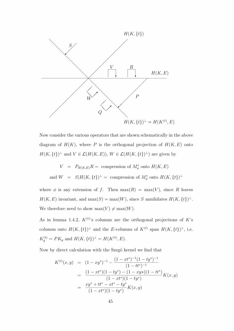
Now consider the various operators that are shown schematically in the above
diagram of H(K), where P is the orthogonal projection of H(K,E) onto
H(K, {t})⊥ and V ∈ L(H(K,E)), W ∈ L(H(K, {t})⊥) are given by
V = PH(K,E)R = compression of M∗φ onto H(K,E)
and W = S|H(K, {t})⊥ = compression of M∗φ onto H(K, {t})⊥
where φ is any extension of f . Then max(R) = max(V ), since R leaves
H(K,E) invariant, and max(S) = max(W ), since S annihilates H(K, {t})⊥.
We therefore need to show max(V ) 6= max(W ).
As in lemma 1.4.2, K(t)’s columns are the orthogonal projections of K’s
columns onto H(K, {t})⊥ and the E-columns of K(t) span H(K, {t})⊥, i.e.
K(t)y = PKy and H(K, {t})⊥ = H(K(t), E).
Now by direct calculation with the Szego kernel we find that
K(t)(x, y) = (1− xy∗)−1 − (1− xt∗)−1(1− ty∗)−1
(1− tt∗)−1
=(1− xt∗)(1− ty∗)− (1− xy∗)(1− tt∗)
(1− xt∗)(1− ty∗)K(x, y)
=xy∗ + tt∗ − xt∗ − ty∗
(1− xt∗)(1− ty∗)K(x, y)
45

=(x− t
1− xt∗)(
y − t1− yt∗
)∗K(x, y)
= bt(x)bt(y)∗K(x, y)
where bt(x) = (x − t)/(1 − xt∗) denotes the Blaschke factor associated with
the point t.
This shows that K(t) is a rank-1 positive Schur multiple of K, so the vectors
{K(t)y : y ∈ E}, which are non-zero since K is completely non-zero, can be
re-scaled so that they have Gram matrix equal to KE. Let Q be the operator
on H(K, {t})⊥ that does this rescaling. Then the vector sets {QK(t)y : y ∈ E}
and {Ky : y ∈ E} have the same Gram matrices and therefore the operator
U : H(K,E)→ H(K, {t})⊥ U = QP = Ky 7→ QK(t)y
is unitary.
But we have
V ∈ L(H(K,E)) V = Ky 7→ f(y)∗Ky y ∈ E
and
W ∈ L(H(K(t), E)) W = K(t)y 7→ f(y)∗K(t)
y y ∈ E
= UKy 7→ f(y)∗UKy y ∈ E.
Therefore, since V and W have the same eigenvalues and U maps V ’s eigen-
vector to W ’s eigenvectors, we have V = U−1WU and so V and W are
unitarily equivalent via the unitary operator U = QP .
Now assume the opposite of what we want to prove, i.e. that max(V ) =
max(W ), and let M denote this common maximising space. Then U must
leave M invariant (since it must map V ’s maximising space to W ’s maximis-
ing space) and so U must have an eigenvector v ∈ M , with corresponding
unimodular eigenvalue λ say. But since M = max(W ) ⊆ H(K, {t})⊥, P
46

has no effect on M , so v must also be an eigenvector of Q with the same
unimodular eigenvalue λ.
But Q already has a spanning set of eigenvectors, namely {K(t)y : y ∈ E},
and the corresponding eigenvalues are all greater than 1 in modulus since
‖QK(t)y ‖ = ‖Ky‖ (since {QK(t)
y : y ∈ E} has Gram matrix K)
> ‖PKy‖ (K(t, y) 6= 0, so Ky is not orthogonal to Kt)
= ‖K(t)y ‖.
Therefore Q cannot also have λ as an eigenvalue. This contradiction proves
that the assumption that max(V ) = max(W ) must be wrong, so completing
the proof.
Since the Szego kernel is NP, uniqueness of one-point extensions implies uniqueness
of extensions to all of D, so we have the following corollary.
Corollary 3.1.3 Let K : D × D → C be the Szego kernel and f : E → C be a
given function on a non-empty, finite subset of D. Then there is a unique minimal
norm extension of f from E to D.
3.2 Blaschke Kernels
In our proof that uniqueness holds for the Szego kernel, lemma 3.1.2, the only
special properties of the Szego kernel that we used, other than it being NP, were
that it is completely non-zero and that K(t) is a rank 1 positive Schur multiple of
K. It is this latter property that is most important—a lot of the rich structure of
H2 stems from this property of its kernel—so we now consider kernels of this type.
We saw in the case of the Szego kernel that the rank 1 Schur multiplier is formed
from the Blaschke factor bt, so I will call these the Blaschke kernels.
47

Definition 3.2.1 A kernel K : X × X → C is a Blaschke kernel if and only if
for each t ∈ X there exists a function bt : X → C such that K(t) = (bt ⊗ b∗t )K.
The functions bt are then called the generalised Blaschke factors associated with the
points of X.
The following two lemmas show what form the Blaschke kernels take.
Lemma 3.2.2 Let K : X ×X → C be a positive-definite kernel. Then there exist
kernels L[t] such that K(t) = L[t]K for each t ∈ X if and only if, for some ordering
of X, K is block diagonal with completely non-zero blocks.
Proof: If such kernels L[t] exist then consider the graph G(K) that has the points
of X as vertices and has an edge connecting x to y whenever K(x, y) 6= 0.
From the equation
K(t) = K(x, y)−K(x, t)K(y, t)∗/K(t, t) = L[t](x, y)K(x, y)
we see that if K(x, y) = 0 then at least one of K(x, t) and K(y, t) must
also be zero, so G(K) has the property that any pair of vertices connected
via a third are also connected directly. G(K) is therefore a union of disjoint
cliques, a clique being a sub-graph with an edge joining every pair of vertices.
Translating this back into the location of zeros in K, this shows that for
some ordering of X, K is block diagonal with completely non-zero blocks, as
claimed.
The reverse implication is clear, since if K is block diagonal with completely
non-zero blocks, then we can define L[t] to be K(t)/K on t’s block and
L[t](x, y) = 1 elsewhere.
48

Lemma 3.2.3 A positive-definite kernel K : X×X → C is a Blaschke kernel if and
only if, for a suitable ordering of X, K is block diagonal with completely non-zero
blocks, each of which is of the form 1/(p⊗ p∗− q⊗ q∗) where p and q are functions
on that block’s domain.
Proof: First assume K is a Blaschke kernel and is therefore, by the previous
lemma, block diagonal with completely non-zero blocks. Consider one of
those blocks, KE say. For x, y ∈ E we can rearrange K(t) = (bt ⊗ b∗t )K as
K(x, y) =K(x, t)K(y, t)∗/K(t, t)
1− bt(x)bt(y)∗=
(1
p⊗ p∗ − q ⊗ q∗
)(x, y)
where
p(x) =√K(t, t)/K(x, t)
q(x) = bt(x)p(x).
K therefore has the claimed form.
Now assume that K is block diagonal and that each block KE has the form
KE = 1/(p⊗ p∗− q⊗ q∗). By lemma 3.2.2, K(t) = L[t]K for some kernel L[t]
and on the block containing t we have
L[t](x, y) = K(t)(x, y)/K(x, y)
= 1− (p(x)p(y)∗ − q(x)q(y)∗)(p(t)p(t)∗ − q(t)q(t)∗)(p(x)p(t)∗ − q(x)q(t)∗)(p(t)p(y)∗ − q(t)q(y)∗)
=p(x)p(y)∗q(t)q(t)∗ + q(x)q(y)∗p(t)p(t)∗ − p(x)q(y)∗p(t)∗q(t)− p(y)∗q(x)p(t)q(t)∗
(p(x)p(t)∗ − q(x)q(t)∗)(p(t)p(y)∗ − q(t)q(y)∗)
=
(p(x)q(t)− q(x)p(t)
p(x)p(t)∗ − q(x)q(t)∗
)(p(y)q(t)− q(y)p(t)
p(y)p(t)∗ − q(y)q(t)∗
)∗= bt(x)bt(y)∗
where
bt(x) =p(x)q(t)− q(x)p(t)
p(x)p(t)∗ − q(x)q(t)∗.
If either of x or y is not in the same block as t then L[t](x, y) = 1, so if we
extend bt from E to X by setting bt(x) = 1 outside E then K(t) = (bt⊗ b∗t )K
on all of X. Therefore K is a Blaschke kernel, as claimed.
49

Note that the generalised Blaschke factor bt is not fully determined by K. On the
block containing the point t it is determined up to a unitary scalar factor. Outside
that block it may take any unitary values, though it is natural to choose the value
1, as we did above.
Finally, let us return to the uniqueness question for Pick’s theorem. We can now
extend our uniqueness result to the completely non-zero Blaschke kernels.
Lemma 3.2.4 Let K : X ×X be a completely non-zero, positive definite, Blaschke
kernel, i.e. a positive definite kernel of the form K = 1/(p⊗p∗−q⊗q∗), where p and
q are any complex-valued functions on X. Then Pick’s theorem is true for H(K)
(i.e. K is NP) and when the data set E is finite the minimal norm interpolating
multiplier is unique.
Proof: K is NP, by theorem 1.5.4, since p ⊗ p∗ − 1/K = q ⊗ q∗ ≥ 0. Therefore
K satisfies all the conditions that we assumed in our argument in proving
lemma 3.1.2, i.e. it is positive-definite, NP, completely non-zero and satisfies
K(t) = (bt ⊗ b∗t )K for some functions bt. Uniqueness therefore holds when E
is finite.
Note that the limitation that K be completely non-zero is certainly necessary.
For otherwise K is block diagonal with more than one block and is effectively
the direct sum of two or more sub-kernels that are completely independent of
each other. Correspondingly, any interpolation problem for K is then equivalent
to two or more simultaneous sub-problems that are independent except that the
overall multiplier norm is the maximum of the norms arising in the sub-problems.
Clearly, in this situation, the overall minimal norm extension will only be uniquely
determined on the critical blocks, i.e. those on which the multiplier achieves its
overall norm.
50

The simplest example of this is the identity kernel on a finite set X, i.e. K(x, y) = 1
if x=y, K(x, y) = 0 otherwise. The multiplier norm is then simply the supremum
norm and we can extend a function f isometrically to a new point t by choosing
any new value ≤ ‖f‖M(K).
51

Chapter 4
The Operator-Valued Case
It is well known [You86, theorem 1] [BGR90] that Pick’s original theorem gener-
alises to operator-valued H∞ spaces. The result can be expressed in the following
form:
Let H be any Hilbert space, and H∞(L(H)) denote the Banach space
of L(H)-valued analytic functions on D with the supremum norm
‖Φ‖∞ = supx∈D‖Φ(x)‖L(H).
Then there exists a function Φ ∈ H∞(L(H)), with ‖Φ‖∞ ≤ 1, that
takes the n given operator values Zi ∈ L(H) at the n given data points
xi ∈ D if and only if the operator matrix(1− ZiZ∗j1− xix∗j
)i,j=1,...,n
is positive.
As in the scalar-valued case covered so far, H∞(L(H)) is the space of multipliers of
H2(H), the space of square-integrable analytic H-valued functions on D, and the
above operator-valued Pick theorem again has a natural possible generalisation
to reproducing kernel Hilbert spaces, this time to vector-valued spaces. In this
chapter I examine how far the method used in chapter 1 generalises to vector-
valued reproducing kernel Hilbert spaces.
52

Sections 1.1 to 1.4 generalise fairly directly, so to ease comparison the corresponding
sections here use the same numbering of lemmas, definitions etc. as in chapter 1.
To avoid repetition I do not go through the arguments step by step, but instead de-
scribe how the results generalise, only going into detail where significant differences
arise.
Section 1.5 does not generalise to the non-commutative world of the operator-
valued case; section 4.5 shows that its results can only really be applied to special
cases where commutativity holds.
4.1 Vector-Valued Reproducing Kernel Spaces
In the generalisation of reproducing kernel Hilbert spaces the kernel becomes
operator-valued and the space becomes one of vector-valued functions. This section
outlines the theory, generally without proof. For further details see [BM84].
Before proceeding, we must define positivity for operator-valued kernels. For my
preferred definition, developed in the beautiful generalisation work of Laurent
Schwartz [Sch64], see chapter 6. However an equivalent, more elementary defi-
nition is as follows. A L(H)-valued kernel K on a finite set X is positive (positive
definite) if and only if the operator on∑x∈X ⊕H with operator matrix K is a posi-
tive (positive definite) operator. This is then extended to infinite sets X by defining
a kernel K to be positive (positive-definite) if and only if all finite restrictions of
K are positive (positive-definite).
Now let X be any set, H be a Hilbert space and K be a positive L(H)-valued
kernel on X ×X. Then for any y ∈ X and any vector h ∈ H, the mapping
K(·, y)h : X → H x 7→ K(x, y)h
defines an H-valued function on X, and as h varies over H this gives a space of
53

functions from X to H
Hy = {x 7→ K(x, y)h : h ∈ H}
which is associated with the y-column of K. The reproducing kernel Hilbert space
generated by K, H(K), is the space of H-valued functions generated by these ‘seed’
spaces Hy. That is
H(K) = span{K(·, y)h : y ∈ X, h ∈ H}
with inner product defined to be the conjugate-linear extension of
〈K(·, y)hy, K(·, x)hx〉H(K) = 〈K(x, y)hy, hx〉H .
The kernel K is called the ‘reproducing’ kernel for H(K) since it has the following
properties with respect to H(K):
• for each y ∈ X and each h ∈ H the function K(·, y)h, obtained by applying
the y-column of K to h, is a member of H(K)
• the functions K(·, y)h (y ∈ X, h ∈ H) ‘reproduce’ all functions f ∈ H(K) in
the sense that
〈f(y), h〉H = 〈f,K(·, y)h〉H(K)
which can be read as
h component of f(y) in H = K(·, y)h component of f in H(K).
Furthermore, H(K) is the only Hilbert space of H-valued functions on X for which
K has these reproducing properties. Conversely, given any Hilbert space of H-
valued functions on a set X, for which all the ‘point-evaluation’ linear operators
from H(K) to H are bounded, there exists a unique positive kernel K on X ×X
with these reproducing properties.
54

To be the kernel of a reproducing kernel Hilbert space the kernel K need only be
positive, not necessarily positive-definite. However, to avoid the unhelpful compli-
cation of degeneracy we will assume from now on that the kernel K is positive-
definite.
Since members of H(K) are H-valued functions, a multiplier of H(K) must be an
L(H)-valued function on X. The multiplier space M(K) is defined to be the space
of L(H)-valued functions on X for which multiplication of H(K) is a bounded
operator. As in the scalar case, both membership and the norms in H(K) and
M(K) can be characterised in terms of positivity, this time positivity of operator-
valued kernels:
• ‖f‖H(K) = infr≥0{r : r2K − f ⊗ f ∗ ≥ 0}
and f ∈ H(K) if and only if this infimum is finite. Here f ⊗ f ∗ is the kernel
whose values are the rank-1 operators given by
(f ⊗ f ∗)(x, y) = f(x)f(y)∗ = h 7→ 〈h, f(y)〉Hf(x).
• ‖Φ‖M(K) = infr≥0{r : r2K − Φ⊗K ⊗ Φ∗ ≥ 0}
and Φ ∈ M(K) if and only if this infimum is finite. Here Φ⊗K ⊗ Φ∗ is the
kernel given by (Φ⊗K ⊗ Φ∗)(x, y) = Φ(x)K(x, y)Φ(y)∗.
Since restrictions of positive operator-valued kernels are positive, it follows from
the above positivity characterisation of ‖ · ‖M(K) that the restriction of a multiplier
in M(K) to a subset E of X is a multiplier in M(KE) with equal or smaller norm.
In the scalar-valued case the columns of K played the role of the ‘reproducing’
functions in H(K)—evaluation of a function in H(K) corresponded to taking its
inner product with the columns of K. They were also used to characterise the
multiplication operator adjoints on H(K) as those that have all these reproducing
functions as eigenvectors. In the operator-valued case, these two roles can be played
55

by the subspaces Hy, by identifying Hy with H via various mappings.
Firstly note that each subspace Hy is unitarily equivalent to H. For, given any
y ∈ X, K(y, y) > 0 so the mapping K(·, y)h 7→ K(y, y)1/2h defines a linear trans-
formation of Hy onto H. But
〈K(·, y)h,K(·, y)k〉H(K) = 〈K(y, y)h, k〉H = 〈K(y, y)1/2h,K(y, y)1/2k〉H
so this mapping is an isometry, and therefore defines a unitary equivalence of Hy
onto H.
Now let Ey denote the operator from Hy to H of evaluation at y. Since
〈K(·, y)h,E∗yh′〉H(K) = 〈EyK(·, y)h, h′〉H
= 〈K(y, y)h, h′〉H
= 〈K(·, y)h,K(·, y)h′〉H(K)
then E∗y is simply multiplication by K(·, y), i.e. E∗y = MKy = h 7→ K(·, y)h.
Letting Py denote the orthogonal projection of H(K) onto Hy, we have
〈f(y), h〉H = 〈f,K(·, y)h〉H(K)
= 〈Pyf,K(·, y)h〉H(K)
= 〈Pyf, E∗yh〉H(K)
= 〈EyPyf, h〉H
so f(y) = EyPyf . In other words, under the (generally non-unitary) identifications
Ey : Hy → H of the subspaces Hy with H, the values of a function in H(K)
are its projections onto the subspaces Hy. This roughly justifies saying that the
subspaces Hy play the role of ‘reproducing’ subspaces of H(K)—projection onto
them evaluates functions in H(K) (under the identifications Ey).
56
4.2 Generalising the Operator Pick Theorem
We now have enough facts and notation to restate a Pick theorem for the operator-
valued case in terms of vector-valued reproducing kernel Hilbert spaces. Let
X = D
K = the operator-valued Szego kernel K(x, y) = IH/(1− xy∗)
E = the set of data points {x1, . . . , xn}
KE = the restriction of K to E
and F = the function on E defined by F (xi) = Zi.
Then H(K) = H2(H) and M(K) = H∞(L(H)) and Pick’s theorem for H∞(L(H))
can be restated as:
(1) There exists a multiplier Φ ∈ M(K) such that Φ|E = F and
‖Φ‖M(K) ≤ 1
if and only if
(2) the L(H)-valued kernel KE − F ⊗KE ⊗ F ∗ is positive.
For general sets X, E ⊆ X, Hilbert space H and positive kernel K on X, this
theorem will be called the generalised operator-valued Pick theorem for H(K) and
we will now investigate for which kernels K it is true.
As in the scalar-valued case, (2) is equivalent to ‖Φ|E‖M(KE) ≤ 1, so (1) ⇒ (2)
is always true, because restricting Φ to E cannot increase its multiplier norm.
The truth of the generalised operator-valued Pick’s theorem therefore depends on
whether (2) ⇒ (1), which is equivalent to always being able to extend multipliers
from subsets of X to the whole of X without increasing multiplier norm.
57

4.3 One-Point Extensions Are Sufficient
The results of section 1.3 generalise fairly directly. Lemma 1.3.1 becomes:
Lemma 4.3.1 Let H be a Hilbert space and K be a positive L(H)-valued kernel on
a set X. Then an operator M on H(K) is a multiplication operator if and only if
the reproducing subspaces Hy are eigenspaces of M∗ for all y ∈ X. Furthermore,
if M is a multiplication operator then the corresponding multiplier Φ is given by
M∗|Hy = MKyΦ(y)∗M−1Ky = K(·, y)h 7→ K(·, y)Φ(y)∗h.
Proof: Given a multiplier Φ ∈M(K)
〈M∗Φ(K(·, y)hy), K(·, x)hx〉H(K) = 〈K(·, y)hy,Φ(·)K(·, x)hx〉H(K)
= 〈hy,Φ(y)K(y, x)hx〉H
= 〈K(x, y)Φ(y)∗hy, hx〉H
= 〈K(·, y)Φ(y)∗hy, K(·, x)hx〉H(K)
and since this is for all x, y ∈ X and all hx, hy ∈ H, we have
M∗Φ(K(·, y)hy) = K(·, y)Φ(y)∗hy.
Therefore M∗Φ leaves Hy invariant and M∗
Φ|Hy = MKyΦ(y)∗M−1Ky , as claimed.
Conversely, if M∗ is a bounded operator on H(K) that leaves Hy invariant
for each y ∈ X, then M∗ and the adjoint of multiplication by the L(H)-
valued function Φ(y)∗ = M−1Ky (M∗|Hy)MKy clearly agree on the reproducing
subspaces Hy, so by linearity and continuity they must also agree on their
closed span, i.e. H(K).
The definition of NP kernels needs no change from that given in chapter 1:
58

Definition 4.3.2 A positive, L(H)-valued kernel K on a set X will be called an
NP kernel provided for every subset E of X and every t ∈ X \E, all multipliers in
M(KE) can be isometrically extended to multipliers in M(KE∪{t}).
Lemma 4.3.3 Given a Hilbert space H and a positive-definite L(H)-valued kernel
K on a set X, then the full Pick theorem is true for H(K) if and only if K is an
NP kernel.
Proof: The proof given in chapter 1 applies equally well in the operator-valued
case, the only places where generalisation are needed being:
• references to columns of a kernel need to be changed throughout to refer
instead to the reproducing subspaces associated with the columns. For
example Hg’s definition becomes ‘the closed subspace of H(KF ) spanned
by the reproducing subspaces of H(KF ) corresponding to Fg’.
• references to eigenvectors need to be changed to eigenspaces
• the above lemma 4.3.1 replaces the use of lemma 1.3.1.
4.4 Minimal Norm Extension
The non-orthogonal generalisation of Parrott’s lemma (1.4.1) developed in chap-
ter 1 is already general enough for the operator-valued case and so stands without
change. However the other results of section 1.4 do need some generalisation.
Lemma 4.4.2 Let K be a positive-definite, L(H)-valued kernel on a set X, t ∈ X,
E = X \ {t} and F be a multiplier of H(KE). Further, let K(t) denote the Schur
complement of K(t,t) in K, given by
K(t)(x, y) = K(x, y)−K(x, t)K(t, t)−1K(t, y).
59

Then ‖F‖M(KE) and ‖F‖M(K
(t)E )
are both lower bounds for the norm of any one-
point extension of F to X, and the larger of the two, if finite, is achievable, i.e.
there exists a one-point extension of F with that norm.
Proof: The proof given for the corresponding lemma (1.4.2) in chapter 1 gen-
eralises fairly directly. To cover this operator-valued case we need to show
that:
• K(t) is the reproducing kernel of the subspace H(K, {t})⊥. To verify
this, note that
〈K(t)(·, y)hy, K(·, t)ht〉H(K)
= 〈K(·, y)hy −K(·, t)K(t, t)−1K(t, y)hy, K(·, t)ht〉H(K)
= 〈K(t, y)hy −K(t, t)K(t, t)−1K(t, y)hy, ht〉H
(using K’s reproducing property)
= 0.
Therefore K(t)(·, y)hy ∈ H(K, {t})⊥ for all y ∈ X. Also
〈f,K(t)(·, y)hy〉 = 〈f,K(·, y)hy −K(·, t)K(t, t)−1K(t, y)hy〉H(K)
= 〈f(y), hy〉H
for all f ∈ H(K, {t})⊥ (using K’s reproducing property and noting that
〈f,K(·, t)K(t, t)−1K(t, y)hy〉H(K) = 0) so K(t) also has the reproducing
property for H(K, {t})⊥.
• the compression W , of TD onto H(K, {t})⊥, leaves the subspaces
{K(t)(·, y)h : h ∈ H} (y ∈ X)
invariant and satisfies
W |{K(t)(·, y)h : h ∈ H} = MK
(t)yF (y)∗M−1
K(t)y
.
60

This is verified by the following calculation.
W (K(t)(·, y)h) = PH⊥2 TD(K(·, y)h−K(·, t)K(t, t)−1K(t, y)h
)= PH⊥2 (A(K(·, y)h)−DK(·, t)K(t, t)−1K(t, y)h)
= PH⊥2 (K(·, y)F (y)∗h) since P⊥H2D = 0
= K(t)(·, y)F (y)∗h.
Lemma 4.4.3 Let K be a positive-definite, L(H)-valued kernel on X, t be any
point of X, E = X \ {t}, and F be a multiplier in M(KE). Then if N is a positive
real such that all restrictions of F to finite subsets G have one-point extensions to
G ∪ {t} with norms ≤ N , there exists an extension of F to X with norm ≤ N .
Proof: The induction proof of the corresponding lemma (1.4.3) in chapter 1 still
works in this operator-valued case, provided we again generalise eigenvectors
to invariant subspaces and eigenvalues to the restrictions of the operator to
those invariant subspaces.
In a little more detail, the operators M∗α are defined as before, again they
form a net in the ball B of radius N in L(H(K)) and since B is compact
there is a cluster point M∗. The new, slightly stronger, fact we now need is
that given a net of operators all of which leave a given subspace invariant and
which all agree on that subspace, then any cluster point of the net must also
share these properties. Using this we can conclude that M∗ must leave all
the reproducing subspaces of H(K) invariant and so, by lemma 4.3.1, be the
adjoint of multiplication by some multiplier Φ. Further, for y ∈ E, M∗|Hy
must equal MKyF (y)∗M−1Ky so Φ|E = F and therefore Φ is an extension of F .
That Φ has multiplier norm ≤ N follows as before.
61

As in chapter 1, it follows from 4.4.3 that for operator-valued kernels we have
‘finitely-NP ≡ NP’ and ‘finite Pick theorem ≡ full Pick theorem’. More precisely:
Corollary 4.4.4 A positive-definite, L(H)-valued kernel K is an NP kernel if
and only if all finite restrictions of K are NP kernels.
Corollary 4.4.5 If K is a positive-definite, L(H)-valued kernel on a set X, then
for H(K) the finite Pick theorem and the full Pick theorem are equivalent.
4.5 Sufficient Conditions for Pick’s Theorem
We have now reached the point where the arguments we used in chapter 1 no
longer generalise fully to the operator-valued case, the barrier basically being non-
commutativity. For example in section 1.5 a key tool used is the Schur product
theorem, i.e. that the pointwise product of two scalar-valued positive kernels is
positive. However this does not hold for two operator-valued positive kernels; for
instance a positive kernel must have positive diagonal entries but the operator
product of two positive operators is not even necessarily Hermitian.
It turns out that the methods from chapter 1 can only be applied if fairly strong
conditions are placed on the operator-valued kernel K, so that commutativity is
restored. Before showing this it will be useful to develop a new view of the one-
point extension method, using the terminology of linear maps on C∗-algebras; this
view will also be needed in the next chapter on completely NP kernels.
For the operator-valued case, consider the problem of isometrically extending a
multiplier F ∈ M(KE) from E = X \ {t} to X. By corollary 4.4.4 we can restrict
attention to the case of X being finite. By lemma 4.4.2 isometric extension will be
possible if and only if
‖multiplication of H(KE) by F‖ ≤ ‖multiplication of H(K(t)E ) by F‖
62

so isometric extension will be possible for all multipliers F ∈M(KE) if and only if
the map
β : M∗F,KE
→M∗F,K
(t)E
is contractive. Here we have extended the notation MF to indicate the space being
multiplied.
LetM(KE) andM(K(t)E ) denote the Banach spaces of multiplication operators on
H(KE) andH(K(t)E ) respectively—M(KE) andM(K
(t)E ) are effectivelyM(KE) and
M(K(t)E ) except that their members are the multiplication operators rather than
the multipliers themselves. These spaces, and the corresponding spaces of adjoints
M(KE)∗ and M(K(t)E )∗, are subspaces of the C∗-algebras L(H(KE)), L(H(K
(t)E ))
and as such are known as operator spaces. The property that interests us, i.e. the
ability to isometrically extend any multiplier, has therefore been characterised in
terms of the contractivity of a linear map β from one operator space onto another.
A lot is known about such maps [Pau86] and in the next chapter this C∗-algebra
way of viewing our problem will prove useful. However, for the moment it is simply
a useful shorthand.
Now consider another way of characterising our property, this time in terms of
positivity of a map operating on kernels. Let γ denote the map
KE − F ⊗KE ⊗ F ∗ 7→ K(t)E − F ⊗K
(t)E ⊗ F ∗
defined on the kernels of the form KE − F ⊗ KE ⊗ F ∗, where F ranges over all
multipliers F ∈M(KE). We know that positivity of the kernels KE−F ⊗KE⊗F ∗
and K(t)E − F ⊗K
(t)E ⊗ F ∗ corresponds exactly to contractivity of F as a multiplier
of H(KE) and H(K(t)E ), respectively, so β is contractive if and only if γ is positive,
i.e. maps positive kernels to positive kernels. In the scalar-valued case (where
everything commutes), and if K is completely non-zero, then γ is simply Schur
multiplication by K(t)E /KE and this allows us to use the Schur product theorem.
63

With this new perspective, we can now summarise the proof of Pick’s theorem
given in chapter 1 as having the following steps.
1. Pick’s theorem is equivalent to always being able to isometrically extend any
multiplier from any given subset E of X to any given extra point t ∈ X \E.
(Shown in sections 1.2 and 1.3.)
2. It is sufficient that isometric extension is always possible when E is finite.
(Shown in section 1.4.)
3. Isometric extension is always possible from E to E ∪ {t} if and only if the
associated map β is contractive. (This was shown, though not in this termi-
nology, in section 1.4.)
4. β is contractive if and only if
γ : KE − F ⊗KE ⊗ F ∗ → K(t)E − F ⊗K
(t)E ⊗ F ∗
is positive. (This is essentially the fact that ‖A‖ ≤ 1⇔ I − A∗A ≥ 0.)
5. When K is completely non-zero, γ is Schur multiplication by K(t)E /KE and so
γ is a positive map if this kernel is positive. (By the Schur product theorem.)
6. K(t)E /KE is positive for each E ⊂ X and t ∈ X \E if and only if κ+(1/K) = 1
(shown in section 1.5). Here
κ+(1/K) = supG⊆X,G finite
(number of positive eigenvalues of (1/K)|G)
is the ‘positivity’ of the kernel 1/K.
From this bird’s eye view of chapter 1’s method we can see how far the method
extends to the operator-valued case now being considered. Steps 1 to 4 generalise
fairly directly, with no special constraints on the kernel K, as has been shown in
sections 4.2 to 4.4. However in step 5 the map
γ : KE − F ⊗KE ⊗ F ∗ → K(t)E − F ⊗K
(t)E ⊗ F ∗
64

will not be a Schur product map unless we can commute the factors KE and K(t)E
out from the centres of the second terms on each side. This will only be possible
for all multipliers F if K is of the form kIH for some scalar-valued kernel k, and to
guarantee γ is a Schur product map k will need to be completely non-zero. We also
need K to be of this form to use the Schur product theorem in step 5, since this
theorem holds for the product of a positive operator-valued kernel by a positive
scalar-valued kernel, but not in general (as noted above) when both kernels are
operator-valued. If K is of the form kIH , with k a completely non-zero scalar-
valued kernel, then γ is Schur multiplication by the scalar-valued kernel k and step
6 for the operator-valued case is exactly as it was for the scalar-valued case.
From this review of chapter 1’s method, and its generalisation to the operator-
valued case, we can see that the method is limited to cases where the operator-
valued kernel K is a scalar multiple of the identity. However, for this case we obtain
the following sufficient conditions for the full Pick theorem to be true for H(K).
Theorem 4.5.1 Let H be a Hilbert space, X be any set and k be a completely
non-zero scalar-valued kernel on X ×X such that κ+(1/k) = 1. Then the full Pick
theorem is true for H(kIH).
Although this result is somewhat limited, it does give as corollaries:
• the original case of Pick’s theorem for H2(H)
• Pick’s theorem for vector-valued Dirichlet spaces.
65

Chapter 5
Completely NP Kernels
Chapter 1 showed that for a completely non-zero, scalar-valued kernel K to be NP
it is sufficient that κ+(1/K) = 1. It is tempting to hope that this condition might
also be necessary and I expended substantial time and effort hoping to prove this,
but only succeeded in proving its necessity for completely non-zero kernels of size
up to 3× 3.
Work by Scott McCullough [McC] then showed that it is better to study a stronger
property than NP-ness, called complete NP-ness. McCullough shows that for com-
pletely non-zero finite kernels the property κ+(1/K) = 1 in fact characterises com-
plete NP-ness rather than the weaker property of NP-ness. In this chapter we
• analyse exactly which are the 3× 3 NP kernels; they are all completely NP
• extend McCullough’s work to a complete characterisation of the completely
NP kernels on any set X
• construct an explicit example of a 4×4 kernel that is NP but is not completely
NP.
66

5.1 Characterisation of 3 by 3 NP Kernels
When working with a finite, scalar-valued, positive-definite kernelK it is convenient
to normalise it by Schur multiplying by a⊗ a∗ where
a(x) = 1/√K(x, x).
This renders all the diagonal terms of K equal to 1 and is equivalent to altering
the norm in H(K) to rescale the reproducing functions to be unit vectors. Be-
cause a multiplication operator adjoint M∗f is the operator with these vectors as
eigenvectors and f(x)∗ as eigenvalues, rescaling the vectors has no effect on the
multiplier norm and so no effect on interpolation questions. We will therefore work
with normalised kernels throughout this section.
When the domain set X is small enough NP-ness of a kernel K can be analysed
by direct hand calculation. The property is meaningless if X contains only one
point since at least two points are needed in order to do a one-point extension. For
the next size up, i.e. card(X) = 2, isometric one point extension of a multiplier
f from {x1} to {x1, x2} is always possible, since we can simply set f(x2) = f(x1).
Therefore all 2× 2 kernels are NP and it is not until card(X) = 3 that interesting
things start to happen.
Take a 3× 3 normalised positive-definite kernel
K =
1 a ba∗ 1 cb∗ c∗ 1
and consider isometrically extending a given multiplier f : {x1, x2} → {f1, f2} by
choosing a value for f3. Let E = {x1, x2} and t = x3. By lemma 1.4.2 this can be
done if and only if
‖f‖M(K
(t)E )≤ ‖f‖M(KE) (?)
and in this case these are multiplier norms associated with 2× 2 kernels so we can
calculate them directly.
67

Let L =
(1 aa∗ 1
)be any positive-definite normalised 2 × 2 kernel on {x1, x2}.
Note that L is positive definite ⇔ det(L) > 0 ⇔ |a| < 1. Then
‖f‖2M(L) = inf(r ≥ 0 : (r − f ⊗ f ∗)L ≥ 0)
= largest root of det
(r − f1f
∗1 a(r − f1f
∗2 )
a∗(r − f2f∗1 ) r − f2f
∗2
)= 0
= largest root of (r − f1f∗1 )(r − f2f
∗2 )− aa∗(r − f2f
∗1 )(r − f1f
∗2 ) = 0
= largest root of r2(1− aa∗)
−r((f1 − f2)(f ∗1 − f ∗2 ) + (1− aa∗)(f1f∗2 + f2f
∗1 ))
+(1− aa∗)|f1|2|f2|2 = 0
= largest root of r2 −Br + C = 0
=B +
√B2 − 4C
2C
where B = |f1 − f2|2/(1− |a|2) + 2<(f1f∗2 ) and C = |f1|2|f2|2.
Although this formula is fairly complicated we can derive from it some useful
information about how ‖f‖M(L) varies with a. Since C is independent of a the
variation only occurs through B. But ‖f‖M(L) is an increasing function of B since
∂(2C‖f‖2M(L))
∂B= 1 +
B√B2 − 4C
=2C‖f‖2
M(L)√B2 − 4C
≥ 0
and B is an increasing function of |a|, so ‖f‖M(L) is an increasing function of |a|.
This tells us how to compare multiplier norms—the larger the off-diagonal term in
the normalised kernel then the larger the multiplier norm.
Applying this to the inequality (?) we see that isometric extension of f will be
possible
⇔ |off-diagonal term in normalised K(t)E |2 ≤ |a|2
⇔ (a− bc∗)(a∗ − b∗c)(1− bb∗)(1− cc∗)
≤ aa∗
since K(t)E =
(1− bb∗ a− bc∗a∗ − b∗c 1− cc∗
)⇔ (a− bc∗)(a∗ − b∗c) ≤ aa∗(1− bb∗)(1− cc∗)
⇔ aa∗bb∗cc∗ − aa∗bb∗ − aa∗cc∗ − bb∗cc∗ + ab∗c+ a∗bc∗ ≥ 0.
68

Because this condition is symmetrical in a, b and c the ability to isometrically
extend all multipliers from 2 points to the third does not depend on which two
points are chosen. Therefore these criteria actually characterise NP-ness of K.
Also, we can see from the form of the inequalities that:
• if exactly one of the off-diagonal terms is zero then K is not NP. For example
if a = 0 then
aa∗bb∗cc∗ − aa∗bb∗ − aa∗cc∗ − bb∗cc∗ + ab∗c+ a∗bc∗ = −bb∗cc∗ 6≥ 0
• if more than one of the off-diagonal terms is zero then K is NP.
• if K is completely non-zero then it is NP if and only if κ+(1/K) = 1. To see
this, note that 1/K must have at least 1 negative and 1 positive eigenvalue
since each of its principal 2 by 2 submatrices have negative determinants.
Therefore the only possible values for κ+(1/K) are 1 and 2 and the latter
value gives
0 > aa∗bb∗cc∗ det(1/K) = aa∗bb∗cc∗− aa∗bb∗− aa∗cc∗− bb∗cc∗+ ab∗c+ a∗bc∗.
We have therefore characterised the 3 × 3 NP kernels—they are the completely
non-zero kernels for which κ+(1/K) = 1 plus the kernels having zeros but which
are block-diagonal. Later in this chapter it will be shown that these are exactly the
completely NP kernels, so for 3 × 3 kernels the adverb ‘completely’ adds nothing
new.
Although the above approach can in principle also be applied to 4 × 4 kernels, in
practice the algebra becomes totally unmanageable—the kernel then has 6 complex
degrees of freedom and a cubic equation must be solved. This is a pity since, as will
be seen in section 5.3, it turns out that in the 4 × 4 case the adverb ‘completely’
does indeed make a difference.
69

5.2 Characterisation of Completely NP kernels
In section 4.5 we introduced a way of viewing NP-ness of a finite kernel K in
terms of a family of maps β defined on operator spaces. Let βK,E,t denote the map
associated with extension from E to t with kernel K, i.e.
βK,E,t :M(KE)∗ →M(K(t)E )∗ M∗
f,KE7→M∗
f,K(t)E
.
Then we know that
K is NP⇔ βK,E,t is contractive for each ∅ ⊂ E ⊂ X and t ∈ X \ E.
From the C∗-algebra viewpoint, the map βK,E,t has some nice properties:
• its domain and range operator spacesM(KE)∗ andM(K(t)E )∗ are unital (they
contain the identity, the adjoint of multiplication by the constant function
1) and are in fact closed non-self-adjoint subalgebras of their respective con-
taining C∗-algebras.
• βK,E,t is unital, i.e. it maps the unit in M(KE)∗ to the unit in M(K(t)E )∗
• βK,E,t is spectrum-preserving and so is a positive map (i.e. maps positive
elements to positive elements). To see this, note that for any positive-definite
kernel L on E, the spectrum of M∗f on H(L) is simply f(E)∗.
This enables us to use the theory of contractivity and positivity of linear maps be-
tween operator spaces in C∗-algebra, which has been made easily accessible by Vern
Paulsen in his very useful book ‘Completely Bounded Maps and Dilations’ [Pau86].
An important role is played in this theory by rather stronger, and better behaved,
properties of C∗-algebra maps called complete contractivity and complete positiv-
ity. Given two C∗-algebras A and B, let Mn(A) and Mn(B) (n ∈ N) denote the
70

induced C∗-algebras of n×n matrices over A and B respectively. Then a linear map
φ : A→ B induces maps φn : Mn(A)→Mn(B) defined by applying φ elementwise:
φn((aij)n1 ) = (φ(aij))
n1
and φ is called completely contractive if all the induced maps φn, n ∈ N, are
contractive. In general, appending the adverb ‘completely’ to a given property of
φ means that φn has that property for each n ∈ N.
This process can equally well be viewed as one of tensor product by the identity of
Mn(C), by making the following identifications:
Mn(A) ' Mn(C)⊗ A
(aij)n1 '
n∑i,j=1
Eij ⊗ aij
φn ' In ⊗ φ
where {Eij : i, j = 1, . . . , n} is the standard basis for Mn(C) and In is the identity
in Mn(C).
In our case the C∗-algebra involved is L(H(K)) and we have
Mn(C)⊗ L(H(K)) = L(Mn(C)⊗H(K)) = L(H(In ⊗K))
where In ⊗K is the operator-valued kernel on X ×X given by
(K ⊗ In)(x, y) = K(x, y)In.
We are therefore led to consider the reproducing kernel Hilbert spaces with kernels
of the form In ⊗ K. Burbea and Masani [BM84] refer to these kernels as the
inflations of K, terminology that I will extend to refer to this general process of
generating larger from smaller, by referring to the spaces Mn(C)⊗A and maps φn
as the inflations of A and φ, respectively.
We can now define complete NP-ness: a kernel K is completely NP if and only if
all of its inflations are NP. The following lemma shows that this is a reasonable use
of the adverb.
71

Lemma 5.2.1 Let K be a positive-definite, scalar-valued kernel on a finite set X.
Then K is completely NP if and only if the maps βK,E,t are completely contractive
for each ∅ ⊂ E ⊂ X and t ∈ X \ E.
Proof: Consider what happens when K is inflated to In⊗K. The inflated Hilbert
space H(In ⊗K) is span{K(·, y)h : y ∈ X, h ∈ Cn} and can be identified as
the direct sum of n copies of H(K), via the identification
K(·, y)ei ' 0⊕ . . .⊕ 0⊕K(·, y)⊕ 0⊕ . . .⊕ 0
where {ei : i = 1, . . . , n} is the standard orthonormal basis of Cn and the
term K(·, y) appears on the right in the i’th position.
The proof of our lemma is now essentially just the (easy, though complicated)
job of following this identification through to the various objects involved in
our study. Under this identification H(In ⊗K) ' ∑n1 ⊕H(K) we find that:
• the algebra of all bounded operators on H(In ⊗K) is identified as the
algebra of n× n matrices with entries taken from L(H(K)). That is
L(H(In ⊗K)) 'Mn ⊗ L(H(K) = the inflation of L(H(K)).
• the y−reproducing subspace of H(In ⊗K) is identified as the subspace
K(·, y)Cn of∑n
1 ⊕H(K).
• the multiplication operator adjoints on H(In ⊗ K) are therefore iden-
tified as the operators on∑n
1 ⊕H(K) that leave each of the subspaces
K(·, y)Cn (y ∈ X) invariant, so they are exactly the n×n matrices with
entries that are operators on H(K) that leave each K(·, y) invariant.
That is
M(In ⊗K)∗ 'Mn(C)⊗M(K)∗ = the inflation of M(K)∗.
72

• the process of inflation commutes with restriction to a subset E ⊂ X.
That is
H((In ⊗K)E) = H(In ⊗ (KE)).
• inflation also commutes with Schur complementation. That is
H((In ⊗K)(t)E ) =
n∑1
⊕H(K(t)E ) = H(In ⊗K(t)
E ).
• βIn⊗K,E,t acts on an operator in M((In ⊗ K)E)∗, which we have seen
can be viewed as an n×n matrix of operators fromM(KE)∗, by simply
applying βK,E,t elementwise. That is
βIn⊗K,E,t ' (βK,E,t)n.
Having identified βIn⊗K,E,t with (βK,E,t)n our result now follows directly since
K is completely NP
⇔ In ⊗K is NP for each n ∈ N
⇔ βIn⊗K,E,t is contractive for all ∅ ⊂ E ⊂ X, t ∈ X \ E, n ∈ N
⇔ (βK,E,t)n is contractive for all ∅ ⊂ E ⊂ X, t ∈ X \ E, n ∈ N
⇔ βK,E,t is completely contractive for all ∅ ⊂ E ⊂ X, t ∈ X \ E.
We can now start to characterise the completely NP kernels by proving, using
our viewpoint and terminology, McCullough’s result for completely non-zero, fi-
nite kernels. The key step in the next proof—the induction step—is derived from
McCullough’s work [McC].
73

Lemma 5.2.2 (S. McCullough) Let K be a completely non-zero positive def-
inite kernel on a finite set X. Then the following are equivalent:
1. K is completely NP.
2. The maps βK,E,t :M(KE)∗ →M(K(t)E )∗ are completely contractive for each
non-empty proper subset E of X and each t ∈ X \ E.
3. K(t)E /KE ≥ 0 for each non-empty proper subset E of X and each t ∈ X \ E.
4. κ+(1/K) = 1.
Proof: Lemma 5.2.1 shows the equivalence of (1) and (2), and in chapter 1 we
showed (lemmas 1.5.1 and 1.5.2) that (3) and (4) are equivalent. It therefore
remains to show that (2) ⇔ (3).
To prove this we will use a matricial representation of the operators involved.
Choose any E ⊂ X, of cardinality n say, and any t ∈ X \E. We can consider
KE as a matrix over Cn, in which case its positive square root K1/2E is such
that its columns are vectors in Cn whose Gram matrix is (K1/2E )∗(K
1/2E ) = KE,
i.e. the same as the reproducing functions in H(KE). The identification
K(·, y) ' y-column of K1/2E
is therefore a Hilbert space isomorphism of H(KE) onto Cn which allows us
to represent H(KE) as Cn.
Using this representation we can form the matrices of operators on H(KE)
with respect to the standard orthonormal basis of Cn. The operator of interest
is the multiplication operator adjoint M∗f , which under our representation
is the operator with the columns of K1/2E as eigenvectors and values f(·)∗
as eigenvalues. With respect to the standard orthonormal basis of Cn, the
matrix of M∗f is therefore
M∗f ' K
1/2E diag(f ∗)K
−1/2E
74

since the matrix K−1/2E maps the columns of K
1/2E to the standard basis
vectors, diag(f ∗) scales them correctly and then K1/2E maps them back again.
We can represent H(K(t)E ) and its operators as Cn and Mn(C) in exactly
the same way. The map βK,E,t is then represented by a linear map on a
subspace of Mn(C). We now have vectorial or matricial representations of all
the elements of our problem:
H(KE) ' Cn
M∗f,KE
' K1/2E diag(f ∗)K
−1/2E
M(KE)∗ ' matrices of the form K1/2E diag(f ∗)K
−1/2E
H(K(t)E ) ' Cn
M∗f,K
(t)E
' K(t)E
1/2diag(f ∗)K
(t)E
−1/2
M(K(t)E )∗ ' matrices of the form K
(t)E
1/2diag(f ∗)K
(t)E
−1/2
βK,E,t ' K1/2E diag(f ∗)K
−1/2E 7→ K
(t)E
1/2diag(f ∗)K
(t)E
−1/2
For brevity, we will now consider the spaces and transformations of the left to
equal those on the right, rather than simply being represented by them. This
is valid since the representations involved preserve all properties of interest.
Also, since K, E and t are now fixed we will now simplify the notation by
omitting the subscripts and simply writing β.
Now consider the following diagram:
M(KE)∗ ⊂Mn(C) -µ
Mn(C)
?
β
?
S
M(K(t)E )∗ ⊂Mn(C) -
νMn(C)
where µ = congruence by K1/2E = A 7→ K
1/2E AK
1/2E
75

ν = congruence by K(t)E
1/2= A 7→ K
(t)E
1/2AK
(t)E
1/2
and S = Schur multiplication by K(t)E /KE.
For any function f : E → C, M∗f,KE
is represented by K1/2E diag(f ∗)K
−1/2E so
(ν−1Sµ)(M∗f,KE
) = (ν−1S)(K1/2E K
1/2E diag(f ∗)K
−1/2E K
1/2E )
= (ν−1S)(KEdiag(f ∗))
= ν−1(K(t)E diag(f ∗))
= K(t)E
1/2diag(f ∗)K
(t)E
−1/2
= βK,E,t(M∗f,KE
).
Therefore β = ν−1Sµ|M(KE)∗; in words, β is congruent to a restriction of
Schur multiplication by K(t)E /KE. We can therefore extend β to a map β on
all of Mn(C) by taking β = ν−1Sµ. β and S are then congruent C∗-algebra
maps via the congruences µ and ν, and because congruences are completely
positive maps (see Paulsen [Pau86, page 28]) the complete positivity of β and
S are equivalent.
There is one more map that we need. Following Paulsen, we extend β to a
map β on the self-adjoint span M(KE)∗ +M(KE) by defining
β(M∗f,KE
+Mg,KE) = β(M∗f,KE
) + β(M∗g,KE
)∗.
The importance of this extension is that β’s domain, being a self-adjoint
subspace, is an operator system, allowing us to use more of Paulsen’s results
on complete positivity and contractivity.
Using the congruence between β and S and the fact that K(t)E /KE is Hermi-
tian, it is easily verified that β is simply β|M(KE)∗+M(KE). We therefore
have the following enlarged commuting diagram.
76

M(KE)∗ ⊂M(KE)∗ +M(KE) ⊂Mn(C) -µ
Mn(C)
?
β
?
β
?
β
?
S
M(K(t)E )∗ ⊂M(K
(t)E )∗ +M(K
(t)E ) ⊂Mn(C) �
ν−1Mn(C)
OperatorSpaces
OperatorSystems
We finally have enough machinery to prove (2)⇔ (3):
(3)⇒(2):
K(t)E /KE ≥ 0 ⇒ S is completely positive, since Schur
multiplication by a positive matrix is
completely positive (see [Pau86, page 31])
⇒ β = ν−1Sµ is completely positive,
since µ and ν−1 are both completely positive
⇒ β is completely positive and so also completely
contractive, since it is unital [Pau86, prop. 3.5].
⇒ β is completely contractive.
(2)⇒(3): We prove this by induction on n, both (2) and (3) being trivially true
for n = 1, so assume the result for size n − 1. Since β is completely
contractive and unital then β is completely positive, by Paulsen [Pau86,
proposition 3.4]. Now consider the effect of β on the positive elements
of {In −∑n
1 A∗iAi : Ai ∈M(KE)∗}. We have
In −n∑1
A∗iAi ≥ 0 ⇔
A1 0 . . . 0A2 0 . . . 0...
.... . .
...An 0 . . . 0
is contractive
77
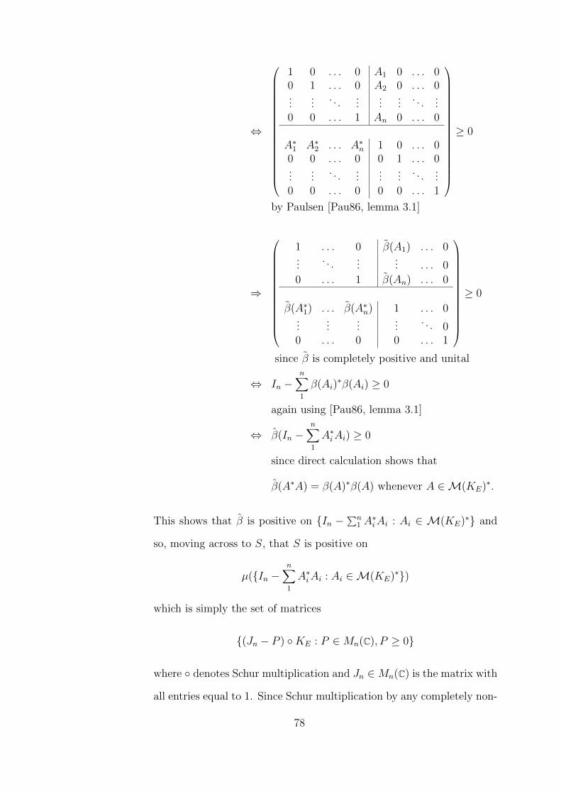
⇔
1 0 . . . 0 A1 0 . . . 00 1 . . . 0 A2 0 . . . 0...
.... . .
......
.... . .
...0 0 . . . 1 An 0 . . . 0
A∗1 A∗2 . . . A∗n 1 0 . . . 00 0 . . . 0 0 1 . . . 0...
.... . .
......
.... . .
...0 0 . . . 0 0 0 . . . 1
≥ 0
by Paulsen [Pau86, lemma 3.1]
⇒
1 . . . 0 β(A1) . . . 0...
. . ....
... . . . 0
0 . . . 1 β(An) . . . 0
β(A∗1) . . . β(A∗n) 1 . . . 0...
......
.... . . 0
0 . . . 0 0 . . . 1
≥ 0
since β is completely positive and unital
⇔ In −n∑1
β(Ai)∗β(Ai) ≥ 0
again using [Pau86, lemma 3.1]
⇔ β(In −n∑1
A∗iAi) ≥ 0
since direct calculation shows that
β(A∗A) = β(A)∗β(A) whenever A ∈M(KE)∗.
This shows that β is positive on {In −∑n
1 A∗iAi : Ai ∈ M(KE)∗} and
so, moving across to S, that S is positive on
µ({In −n∑1
A∗iAi : Ai ∈M(KE)∗})
which is simply the set of matrices
{(Jn − P ) ◦KE : P ∈Mn(C), P ≥ 0}
where ◦ denotes Schur multiplication and Jn ∈Mn(C) is the matrix with
all entries equal to 1. Since Schur multiplication by any completely non-
78

zero, rank-1, positive matrix is a positive map with positive inverse, S
must also be positive on
{(P1 − P ) ◦KE : P1 completely non-zero, rank-1 and ≥ 0, P ≥ 0}.
Now, since K is completely NP so is KE. Hence, by the induction
hypothesis κ+(1/KE) = 1, so
1/KE = P1 − P
where P1 ≥ 0, P ≥ 0 and rank(P1) = 1. Moreover P1 must be completely
non-zero, since otherwise it would have a zero diagonal entry and the
corresponding diagonal entry of KE would be ≤ 0. Hence
Jn = (P1 − P ) ◦KE
is a positive matrix contained in the set on which S is positive, so
K(t)E /KE = S(J) ≥ 0. Since this is true for all proper subsets E of
X the induction step is complete.
We can now characterise the completely NP kernels.
Theorem 5.2.3 Let K be a scalar-valued positive definite kernel on a set X. Then
K is completely NP if and only if for some ordering of the points of X, K is
block-diagonal with each block, Kα say, being completely non-zero and such that
κ+(1/Kα) = 1.
Proof: ⇐ Let K be a block diagonal with completely non-zero blocks
Kα : Xα → C
satisfying κ+(1/Kα) = 1. Then for each n ∈ N, H(In⊗K) is simply the
orthogonal direct sum of the spaces H(In ⊗Kα). Consider attempting
79

to isometrically extend a given multiplier F : E → C of H(In ⊗K) to
a new point t that is in block αt say. MF is simply the direct sum of
the operators MFα , where Fα = F |E ∩ Xα, and F ’s multiplier norm is
therefore simply the largest of the multiplier norms of the functions Fα.
The problem of isometrically extending F to t therefore reduces to that
of isometrically extending Fαt . This is indeed possible if X is finite, since
then Kαt is completely NP, by the previous lemma, so In⊗K is therefore
NP. If X is infinite, the argument only shows that all finite restrictions
of In ⊗K are NP, but then In ⊗K is itself NP, by corollary 4.4.4. We
have therefore shown that all the inflations of K are NP, i.e. that K is
completely NP.
⇒ Form the graph G(K), associated with K, with the points of X as vertices
and having vertices x and y joined by an edge if and only if K(x, y) 6= 0.
(Since K is Hermitian K(x, y) 6= 0⇔ K(y, x) 6= 0.)
Now consider any two vertices x and y that are joined via a third vertex
a, i.e. K(a, x) 6= 0 and K(a, y) 6= 0. Then K{a,x,y} is a completely NP
kernel of the form K(a, a) 6= 0 K(a, x) 6= 0 K(a, y) 6= 0K(x, a) 6= 0 K(x, x) 6= 0 K(x, y)K(y, a) 6= 0 K(y, x) K(y, y) 6= 0
so by section 5.1 K(x, y) must also be non-zero. It follows that in G(K)
any two vertices that are joined via any path along edges are also joined
directly by an edge. In other words G(K) is a union of disjoint cliques
(a clique being a sub-graph with an edge joining every pair of vertices).
Translating this back into the location of zeros in K, this shows that
K is block diagonal, with completely non-zero blocks Kα say, for some
ordering of the points of X, as claimed.
Finally, since all restrictions of completely NP kernels are completely
NP, every finite restriction, L say, of each block Kα is completely NP
80
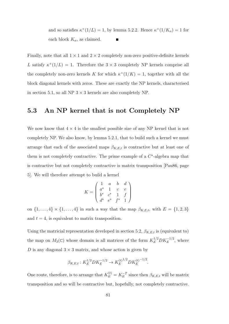
and so satisfies κ+(1/L) = 1, by lemma 5.2.2. Hence κ+(1/Kα) = 1 for
each block Kα, as claimed.
Finally, note that all 1× 1 and 2× 2 completely non-zero positive-definite kernels
L satisfy κ+(1/L) = 1. Therefore the 3 × 3 completely NP kernels comprise all
the completely non-zero kernels K for which κ+(1/K) = 1, together with all the
block diagonal kernels with zeros. These are exactly the NP kernels, characterised
in section 5.1, so all NP 3× 3 kernels are also completely NP.
5.3 An NP kernel that is not Completely NP
We now know that 4× 4 is the smallest possible size of any NP kernel that is not
completely NP. We also know, by lemma 5.2.1, that to build such a kernel we must
arrange that each of the associated maps βK,E,t is contractive but at least one of
them is not completely contractive. The prime example of a C∗-algebra map that
is contractive but not completely contractive is matrix transposition [Pau86, page
5]. We will therefore attempt to build a kernel
K =
1 a b da∗ 1 c eb∗ c∗ 1 fd∗ e∗ f ∗ 1
on {1, . . . , 4} × {1, . . . , 4} in such a way that the map βK,E,t, with E = {1, 2, 3}
and t = 4, is equivalent to matrix transposition.
Using the matricial representation developed in section 5.2, βK,E,t is (equivalent to)
the map on M3(C) whose domain is all matrices of the form K1/2E DK
−1/2E , where
D is any diagonal 3× 3 matrix, and whose action is given by
βK,E,t : K1/2E DK
−1/2E → K
(t)E
1/2DK
(t)E
−1/2.
One route, therefore, is to arrange that K(t)E = K−TE since then βK,E,t will be matrix
transposition and so will be contractive but, hopefully, not completely contractive.
81

(We cannot guarantee that βK,E,t will not be completely contractive, since βK,E,t’s
domain is not all of M3(C).)
We have
det(KE)K−TE =
1− cc∗ b∗c− a∗ a∗c∗ − b∗bc∗ − a 1− bb∗ b∗a− c∗ac− b ba∗ − c 1− aa∗
and
K(t)E =
1− dd∗ a− de∗ b− df ∗a∗ − d∗e 1− ee∗ c− ef ∗b∗ − d∗f c∗ − e∗f 1− ff ∗
.Therefore if we choose d = c∗, e = b, f = a and a and b real then
det(KE)K−TE =
1− cc∗ bc− a c∗a− bbc∗ − a 1− b2 ab− c∗ca− b ab− c 1− a2
and
K(t)E =
1− cc∗ −(bc− a)∗ −(c∗a− b)−(bc∗ − a)∗ 1− b2 −(ab− c∗)∗−(ca− b) −(ab− c)∗ 1− a2
so that all the terms have the correct magnitude. All that remains is to align the
phases of the off-diagonal terms and to do this we can Schur multiply K(t)E by a
rank-1 positive of the form (uiu∗j) where the ui, i = 1, . . . , 3, are unitary scalars.
The effect of this is to add
φ(u1)− φ(u2) to (K(t)E )12
φ(u2)− φ(u3) to (K(t)E )23
and φ(u3)− φ(u1) to (K(t)E )31
where φ(·) denotes the phase of a complex number. We cannot adjust the phases
of the 3 above-diagonal terms in KE independently, since the phase shifts achieved
must sum to zero. In fact we can choose suitable ui to achieve the desired phases
⇔ φ(bc− a)− φ(−(bc− a)∗)
+φ(ab− c∗)− φ(−(ab− c∗)∗)
+φ(c∗a− b)− φ(−(c∗a− b)) = 0 (mod 2π)
82

⇔ π − 2φ(−(bc− a)∗) + π − 2φ(−(ab− c∗)∗) + π = 0 (mod 2π)
⇔ φ(a− bc∗) + φ(c− ab) = 3π/2 (mod 2π)
⇔ φ((a− bc∗)(c− ab)) = 3π/2 (mod 2π)
⇔ φ((ax− a2b− bx2 − by2 + ab2x) + i(ay − ab2y)) = 3π/2 (mod 2π)
where c = x+ iy.
Finally, to arrange this last condition we can choose
0 < a, 0 < b < 1 and y = −√
(ax− a2b− bx2 + ab2x)/b
since this gives
(a− bc∗)(c− ab) = −ia(1− b2)√
(ax− a2b− bx2 + ab2x)/b
and one simple way to achieve this is to take
0 < a = b = x < 1 y = −√x− 2x2 + x3 = −(1− x)
√x.
These values, together with the values d = c∗, e = b and f = a chosen earlier, give
K =
1 x x x+ i(1− x)
√x
x 1 x− i(1− x)√x x
x x+ i(1− x)√x 1 x
x− i(1− x)√x x x 1
so this kernel is such that K
(t)E is a completely non-zero, rank-1 Schur multiple of
K−TE . As mentioned earlier, the rank-1 Schur multiple has no effect on the multiplier
norm, so in terms of contractivity βK,E,t is now equivalent to a restriction of matrix
transposition and so is contractive (but we hope not completely so).
Therefore isometric extension of any multiplier from the first three points to the
fourth is always possible. Further, because of K’s strong symmetry it is easy to see
by row and column swapping that the same must be true for extension from any
three points to the remaining point. If we now take x = 14
as a particular example,
numerical calculations show that
κ+(1/K{1,2,3}) = κ+(1/K{2,3,4}) = κ+(1/K{3,4,1}) = κ+(1/K{4,1,2}) = 1
83

so each of the 3×3 principle subkernels are completely NP. Therefore all one-point
extensions of multipliers can be done isometrically and so this does indeed give an
NP kernel.
However we find by direct calculation that
κ+(1/K) = 2
so K is not completely NP. Therefore
K =
1 1
414
14
+ 3i8
14
1 14− 3i
814
14
14
+ 3i8
14
14
14− 3i
814
14
1
is an explicit example of an NP kernel that is not completely NP.
84

Chapter 6
Generalised Kernels
So far, our use of reproducing kernels has been based on Aronszajn’s paper[Aro50]
linking the positive kernels on a set X with the Hilbert spaces of functions on X.
The positivity of the inner product in such a space stems directly from the positivity
of the kernel, so it is natural to hope that this link between kernels and spaces can
be extended to one between the Hermitian kernels on X and the indefinite inner
product spaces of functions on X. One would then expect the Hermitian kernels
of finite negativity to give rise to reproducing kernel Pontrjagin spaces and those
of infinite negativity to give reproducing kernel Kreın spaces.
In 1964 Laurent Schwartz showed that such a link does indeed exist[Sch64], pro-
vided we restrict ourselves to Hermitian kernels that are the difference of two
positive kernels. Schwartz’s brilliant paper in fact does much more than this—it
explores and generalises the whole area of kernels and associated spaces—but un-
fortunately seems to have been missed by the literature on reproducing kernels. As
a result, the extension of Aronszajn’s work to reproducing kernel Pontrjagin spaces
was later independently proved by Sorjonen[Sor75] and even later, and again inde-
pendently, by Alpay[AD]. Alpay later discovered Schwartz’s work and brought it
to my attention.
This chapter is a short interlude from interpolation questions, with a twofold pur-
85

pose:
• to briefly describe Schwartz’s approach and results, since they give great
insight into reproducing kernels.
• to use his approach to prove a result on the inertia of kernels, which we will
need in the next chapter.
6.1 Schwartz Kernels
Schwartz’s kernels are more general beasts than Aronszajn’s—they are operators on
topological vector spaces—so we must start with some definitions. Let E be any
locally convex, quasi-complete, Hausdorff topological vector space, where quasi-
complete means that all closed bounded subsets are complete. We denote by E ′
the conjugate dual of E, i.e. the space of all continuous linear functionals on E
endowed with pointwise addition and the conjugated scalar multiplication given by
(λf)(e) = λ∗f(e) (e ∈ E, f ∈ E ′, λ ∈ C).
Although E starts with a given topology we will always work with the weak topol-
ogy induced on E by E ′; similarly on E ′ we will use the weak topology induced
by E, i.e. the weakest topology that makes all the point evaluation functionals
continuous.
A Schwartz kernel relative to E is any weakly continuous linear operator from E ′
to E. We can add, subtract and scalar multiply Schwartz kernels in the usual
pointwise manner.
Because we are using the conjugate dual of E, the natural scalar product of elements
from E and E ′ given by (e, f) = f(e) (e ∈ E, f ∈ E ′) is a conjugate-linear product.
The interaction between this scalar product and the weakly continuous operators
from E ′ to E closely follows that between the inner product on a Hilbert space and
86
the operators on that space. For example we can define the adjoint of a kernel K
to be the kernel K∗ given by
(K∗f1, f2) = (Kf2, f1)∗ whenever f1, f2 ∈ E ′
and call K Hermitian if and only if K∗ = K and positive, denoted K ≥ 0, if
and only if (Kf, f) ≥ 0 for all f ∈ E ′. As with operators on Hilbert spaces, the
positive kernels are all Hermitian and form a convex cone (using the partial order
L ≥ K ⇔ L−K ≥ 0) in the space of all kernels relative to E.
Given a Hermitian kernel K we can define an inner product 〈·, ·〉 on ran(K) by
〈Kf,Kg〉 = (Kf, g) = g(Kf). Because K is Hermitian this is well-defined, since
if Kf = Kf1 and Kg = Kg1 we have
〈Kf1, Kg1〉 = (Kf1, g1) by definition
= (Kf, g1)
= (Kg1, f)∗ since K∗ = K
= (Kg, f)∗
= (Kf, g) again since K∗ = K
= 〈Kf,Kg2〉.
However, although this is an inner product space naturally associated with the
Hermitian kernel K, we wish to associate a complete space with K and as yet we
have no topology defined on ran(K).
Now suppose K is positive rather than just Hermitian; then this inner product on
ran(K) is positive-definite and so induces a norm and a topology. Schwartz shows
that, with this topology, ran(K) has a unique completion that is continuously
embedded in E. This completion is called the reproducing kernel Hilbert space
associated with K, denoted H(K), since for it the kernel K satisfies the following
87

reproducing property:
f(e) = 〈e,Kf〉 whenever e ∈ H(K) and f ∈ E ′.
Schwartz shows that the spaces H(K) that arise from the positive kernels are
exactly those Hilbert spaces that are continuously embedded in E (from the norm
topology on H(K) to the weak topology on E). Indeed, on the set of such spaces,
denoted Hilb(E), he defines the following partial order, addition, multiplication by
non-negative reals
• H1 ≤ H2 ⇔ H1 is contractively embedded in H2
• H1 +H2 = span(H1, H2) with norm ‖h‖2 = infh=h1+h2 ‖h1‖2 + ‖h2‖2
• λH = H with the inner product scaled by 1/λ (λH = {0} if λ = 0)
and shows that Hilb(E) is then a convex cone which is isomorphic to the cone of
positive kernels via the identification K ↔ H(K). This isomorphism allows us
to translate between an operator-theoretic view and a spatial view; for example it
tells us that if K and L are two positive kernels relative to E then K ≤ L if and
only if H(K) is contractively embedded in H(L).
Before we consider non-positive Hermitian kernels, it is worth noting that under this
approach any Hilbert space H can be considered as a reproducing kernel Hilbert
space, simply by taking E to be any locally convex, quasi-complete, Hausdorff
topological vector space in which H is continuously embedded. One important
example is to take E to be a Hilbert space containing H. E is then self-dual and if
we use the natural identification of E ′ with E then H’s reproducing kernel relative
to E is simply TT ∗, where T is the embedding of H in E. There are therefore
many possible choices for E, and H has many reproducing kernels, exactly one for
each possible choice for E.
88

6.2 Reproducing Kernel Kreın Spaces
We have seen above that there is a one-to-one correspondence between the positive
kernels relative to E and the Hilbert spaces continuously embedded in E. Things
do not work out quite so neatly when this is extended to non-positive Hermitian
kernels. Here is a summary of Schwartz’s results:
• Each Kreın space H that is continuously embedded in E (from the strong
topology on H to the weak topology on E) has a unique corresponding re-
producing Hermitian kernel K, which can be expressed as the difference of
two positive kernels. I will call a kernel that can be so expressed a splittable
kernel.
• Depending on E there may exist Hermitian kernels which are not splittable,
in which case they do not have any corresponding reproducing kernel Kreın
spaces.
• Each splittable Hermitian kernel K is the reproducing kernel for at least one
Kreın space continuously embedded in E. In general there may be many such
spaces with the same reproducing kernel, in which case Schwartz calls K a
kernel of multiplicity. If there is only one he calls K a kernel of uniqueness
and only in this case can we refer to the reproducing kernel space with kernel
K and use the notation H(K) unambiguously.
• Two positive kernels K and L are called independent if H(K)∩H(L) = {0}.
A splittable Hermitian kernel K can always be expressed as the difference of
two independent positive kernels.
• If a Hermitian kernel K can be split into the difference of two positive kernels
such that one of them is of finite rank then K is a kernel of uniqueness. In
89

other words, distinct Pontrjagin spaces continuously embedded in E have
distinct reproducing kernels, which are kernels of uniqueness.
For a splittable Hermitian kernel K these results allow us to define the positivity
κ+(K) and negativity κ−(K) to equal the dimensions of any maximal positive-
definite and negative-definite subspaces, respectively, of any of its corresponding
reproducing kernel Kreın spaces. There is no ambiguity here since if there is a
choice here for the Kreın space they must all have infinite positivity and infinite
negativity.
In the case described earlier where E is a Hilbert space and K = TT ∗, T being
the embedding of H(K) in E, these definitions of κ− and κ+ coincide with the
usual definitions of the negativity and positivity of the Hermitian operator TT ∗.
That is κ−(TT ∗) and κ+(TT ∗) equal the dimensions of the spectral subspaces
corresponding to (−∞, 0) and (0,∞) respectively. The definitions also agree with
the more elementary definitions given earlier for the negativity and positivity of a
scalar-valued Aronszajn kernel. That is
κ±(K) = supF finite
number of +ve/-ve eigenvalues of KF .
6.3 Relationship to Aronszajn’s Kernels
To see how Schwartz’s kernels generalise Aronszajn’s we must choose E to be the
vector space CX of all complex-valued functions on the domain set X, with the
weak topology, i.e. that of pointwise convergence. E ′ is then simply the finite
linear span of the point evaluation functionals and can therefore be identified with
the space of all finitely-supported functions on X by taking a finitely-supported
function f to correspond to the linear functional on E given by
e 7→∑
x∈support(f)
f(x)e(x).
90

Using this identification the Dirac delta functions {δx : x ∈ X} correspond to the
point evaluation functionals and E ′ is simply span{δx : x ∈ X}, a dense subspace
of E.
The delta functions form a natural basis for both E ′, which they span, and also
for E, of which they span a dense subspace, and with respect to these bases the
weakly continuous linear operator from E ′ to E correspond exactly to the set of
all X × X matrices. The Aronszajn kernels on X are hence simply the matrices,
with respect to these bases, of the Schwartz kernels relative to CX .
6.4 Negativity of Kernel Differences
If K and L are two positive Schwartz kernels relative to E, we know from Schwartz’s
results that L−K ≥ 0 if and only if H(K) is contractively embedded in H(L), but
what happens if L−K is not positive? In this section we use Schwartz’s results to
obtain a result that we will need in the next chapter, namely a characterisation of
κ−(L−K) in terms of the relationship between H(K) and H(L). Our approach is
to first prove the corresponding result for Hilbert space operators, by generalising
Douglas’s lemma, and then extend this to Schwartz kernels.
Lemma 6.4.1 In the following diagram let A and B be given bounded linear oper-
ators between Hilbert spaces F , G and H.
H F
G
-A
?
B
����������
Z
91

Then
κ−(B∗B − A∗A) = min‖Z‖≤1
rank(A− ZB).
Note that ∞ is a possible value for each side.
Proof: We will first show that
κ−(B∗B − A∗A) ≤ min‖Z‖≤1
rank(A− ZB).
Let Z : G→ F be any contraction, J = ker(A− ZB), k = rank(A− ZB) =
codim(J) and assume k <∞. Then for any h ∈ J we have
〈(B∗B − A∗A)h, h〉 = ‖Bh‖2 − ‖Ah‖2
= ‖Bh‖2 − ‖ZBh‖2 since h ∈ ker(A− ZB)
≥ ‖Bh‖2 − ‖Bh‖2 since Z is a contraction
= 0
so (B∗B − A∗A)|J is positive. Hence J must have trivial intersection with
the spectral subspace of B∗B − A∗A corresponding to (−∞, 0), on which
B∗B−A∗A is negative definite, so that spectral subspace must have dimension
≤ k. Therefore κ−(B∗B − A∗A) ≤ k, as claimed.
Conversely, to show
κ−(B∗B − A∗A) ≥ min‖Z‖≤1
rank(A− ZB)
let κ−(B∗B −A∗A) = k <∞ and J be the spectral subspace of B∗B −A∗A
corresponding to [0,∞). Then (B∗B − A∗A)|J is positive, so define Z on
B(J) by Zx = Ay where y is any vector in J for which x = By. This defines
Zx unambiguously since if y′ ∈ J is another such vector then
0 ≤ ‖Ay − Ay′‖2 = 〈A∗A(y − y′), y − y′〉
≤ 〈B∗B(y − y′), y − y′〉
= ‖B(y − y′)‖2
= 0.
92

Also, Z is contractive on B(J) since for x ∈ B(J)
‖Zx‖2 = ‖Ay‖2 = 〈A∗Ay, y〉 ≤ 〈B∗By, y〉 = ‖By‖2 = ‖x‖2.
We can now extend Z to a contraction on the whole of G, by extending by
continuity to the closure of B(J) and then by zero extension to the orthogonal
complement that remains. For the resulting contraction Z we have that
J ⊆ ker(A− ZB), so
rank(A− ZB) = codim(ker(A− ZB)) ≤ codim(J) = κ−(B∗B − A∗A) = k.
Therefore κ−(B∗B − A∗A) ≥ min‖Z‖≤1 rank(A − ZB) as claimed and the
proof is complete.
We can now extend this to differences of Schwartz kernels.
Theorem 6.4.2 Let K and L be positive Schwartz kernels relative to a locally
convex, quasi-complete, Hausdorff topological vector space E. Then
κ−(L−K) = min(codim(J))
where the minimum is taken over all closed subspaces J of H(K) that are contrac-
tively embedded in H(L).
Proof: Apply the above generalised Douglas’s lemma with
H = any member H(M) of Hilb(E) that contains H(K) and H(L).
For example taking M = K + L will suffice.
F = H(K)
G = H(L)
A∗ = embedding of H(K) in H(M)
B∗ = embedding of H(L) in H(M).
93

H(M) H(K)
H(L)
-A�
A∗
?
B
6
B∗
���������
Z
Because H(K) and H(L) are continuously embedded in H(M) we can con-
sider their kernels relative to H(M) as well as relative to E. They are A∗A
and B∗B, respectively, and by Schwartz’s results [Sch64, Proposition 21] we
also have that K = A∗AM and L = B∗BM .
Now let H be a Kreın space continuously embedded in H(M) whose kernel
relative to H(M) is B∗B − A∗A; there is at least one such. Since H(M) is
continuously embedded in E so is H. Moreover, again by Schwartz [Sch64,
Proposition 21], its kernel relative to E is B∗BM − A∗AM = L − K. In
other words B∗B − A∗A and L−K are the kernels of the same Kreın space
H relative to two different containing topological vector spaces. Hence they
must have the same negativity, i.e. κ−(L−K) = κ−(B∗B − A∗A).
Having changed our underlying topological space from E to the Hilbert space
H(M) we can now apply lemma 6.4.1, giving
κ−(L−K) = κ−(B∗B − A∗A) = min‖Z‖≤1
rank(A− ZB)
= min‖Z‖≤1
codim(ker(A− ZB))
= min‖Z∗‖≤1
codim(ker(A∗ −B∗Z∗)).
But if Z∗ : H(K)→ H(L) is a contraction then for all v ∈ ker(A∗ −B∗Z∗)
v = A∗v since A∗ is the embedding of H(K) into H(M)
94

= B∗Z∗v since v ∈ ker(A∗ −B∗Z∗)
= Z∗v since B∗ is the embedding of H(L) into H(M)
so Z∗ contractively embeds ker(A∗−B∗Z∗) in H(L). This argument is clearly
reversible, so the contractive embeddings of closed subspaces of H(K) into
H(L) correspond exactly to contractions Z∗ : H(K) → H(L) and the as-
sociated spaces ker(A∗ − B∗Z∗). Therefore, as claimed, κ−(L − K) equals
the smallest possible codimension of any closed subspace of H(K) that is
contractively embedded in H(L).
Our detour into Schwartz’s work has enabled us to prove the above theorem, which
we will need in the next chapter. However, we will not otherwise use the huge gener-
ality of Schwartz’s kernels—in all that follows the kernels considered are Aronszajn
kernels, i.e. matrices over a set X.
95
Chapter 7
The Adamyan-Arov-KreınTheorem
From our reproducing kernel viewpoint, Pick’s theorem is that ‖Mf‖ is the smallest
possible norm of any bounded analytic function on D that interpolates f : E → C,
where Mf is the operator on H(KE) of multiplication by f and K is the Szego ker-
nel on D. ‖Mf‖ is the first singular value of Mf and in 1971 V.M. Adamyan, D.Z.
Arov and M.G. Kreın [AAK71] proved a result which showed that further infor-
mation about ‘smallest’ interpolating functions can be extracted from the operator
Mf by looking at its other singular values. This chapter develops a reproducing
kernel Hilbert space approach to proving their result and studies whether it can be
generalised to multipliers of other reproducing kernel Hilbert spaces.
7.1 Introduction
The Adamyan-Arov-Kreın theorem (AAK theorem for short) is not, in its original
form, an interpolation result. However it can be reformulated as one and it is
this form that we will state and work on throughout. To state the AAK theorem
accurately we need to make some definitions. Firstly we define notation for singular
values. Let s0(A), s1(A), . . . denote the singular values of an operator A on a Hilbert
96

space H, defined by
sk(A) = inf ‖A|J‖
where the infimum is over all closed subspaces J of H of codimension ≤ k. We will
be working almost exclusively with multiplication operators on reproducing kernel
Hilbert spaces, so for convenience we will extend the concept of singular values to
apply to functions, as follows. Relative to a given positive-definite kernel K on a
set X, we define the singular values of any function f on a non-empty subset E of
X by
sk(f,K) = inf ‖Mf : J → H(KE)‖
where J ranges over all closed subspaces of H(KE) of co-dimension ≤ k. Of course
when E is infinite, multiplication by f may not map J into H(KE) or else may do
so unboundedly; in these cases we take the norm in the definition to be ∞. The
singular values of a function relative to a kernel are hence a decreasing sequence
of non-negative real or infinite values. Since the underlying kernel K we use will
always be fixed, we will usually abbreviate sk(f,K) to sk(f).
Secondly, let bt = (z − t)/(1 − zt∗) denote the Blaschke factor associated with
the point t ∈ D and, for each k ∈ N, let Bk denote the set of Blaschke products
with up to k factors, i.e. the functions of the form bt1bt2 . . . bti for some set of (not
necessarily distinct) points t1, . . . , ti (i ≤ k) in the disc. Note that, for convenience,
we will take the constant function 1 to be the (unique) Blaschke product with no
factors, so B0 = {1}.
We can now state the AAK theorem in the form that we will prove:
Let K be the Szego kernel and f : E → C be any given function on a
non-empty subset E of D. Then for each k = 0, 1, . . .
sk(f) = min ‖φ‖∞
97

where the minimum is taken over all φ ∈ H∞ such that φ|E = fb|E for
some b ∈ Bk or is taken to be ∞ if there is no such φ.
I have expressed the theorem here in a very compact form, but at the cost of
masking what it tells us about functions that interpolate f . To obtain information
about interpolating f we must divide the equation φ|E = fb|E through by b, so
let us examine what happens when we do this.
Assume first that b has no zeros in E. Then (φ/b)|E = f and so φ/b is a mero-
morphic function, with at most k poles, which interpolates f and has supremum
norm sk(f) around the disc edge (since b is unimodular there). What happens if b
has a zero in E, at α say? Then φ(α) = b(α)f(α) = 0 so when we divide through
b’s zero at α is cancelled by φ’s zero there so φ/b has one less pole. However, to
compensate for φ/b being, as it were, one step nearer to analyticity, we no longer
know that (φ/b)(α) = f(α) so we are possibly one step away from interpolating f .
This pattern continues when b has multiple zeros in E; for each zero in E, φ/b has
one less pole but has one more possible interpolation failure.
These arguments all turn out to be reversible, so when the AAK theorem is in-
terpreted as a statement about interpolating f with a meromorphic function it
says
sk(f) is the smallest possible supremum norm (around the disc edge) of
any meromorphic function on D that has a total of at most k failures of
analyticity or points where it fails to interpolate f . If there is no such
function then sk(f) =∞.
When E is finite, the zeros of b are often all outside E and then an interpolating
meromorphic function is obtained. Because of this the AAK theorem is sometimes
thought of as saying that f can be interpolated by a meromorphic function that
98

is bounded by sk(f) around the disc edge and has at most k poles, but this is
not always true. A simple counter-example is obtained by taking E to have k or
fewer points. Then multiplication of H(KE) by f has rank ≤ k, so sk(f) = 0 and
therefore φ must be zero around the disc edge. Being meromorphic, φ must be the
zero function, so in this case φ is analytic but fails to interpolate f wherever it is
non-zero.
It is easy to overlook the possibility that b may have zeros in E. This is why I
have preferred to state the AAK theorem in terms of an analytic function φ that
interpolates fb|E. In this form the k ‘failures’ of analyticity or interpolation are
treated equally—they are simply zeros of b.
7.2 Kernel Characterisation of sk
An important tool in our proof of Pick’s theorem was the characterisation of the
multiplier norm in terms of kernel positivity:
s0(f) = ‖f‖M(K) = infr≥0
(r : (r2 − f ⊗ f ∗)K ≥ 0).
Before we can tackle the AAK theorem we will need the corresponding tool for the
case k > 0, given by the following lemma.
Lemma 7.2.1 Let X be any non-empty set and K : X × X → C be a positive
definite kernel on X. Then the singular values of a function f : X → C relative to
K are given by
sk(f) = infr≥0
(r : κ−((r2 − f ⊗ f ∗)K) ≤ k) k = 0, 1, . . .
and the infimum, if finite, is attained.
Proof: Consider the space Mf (H(K)), the image of H(K) under multiplication
99

by f , endowed with the inner product defined by
〈fh1, fh2〉 = 〈h1, h2〉H(K) whenever h1, h2 ∈ H(K) ker(Mf ).
Direct calculation confirms that (f ⊗ f ∗)K has all its columns in Mf (H(K))
and satisfies the reproducing property for the inner product defined, so this
space is H((f ⊗ f ∗)K). In other words, H((f ⊗ f ∗)K) is simply the image
of H(K) under multiplication by f , given the inner product mapped across
from H(K) ker(Mf ) unitarily by Mf .
For any subspace J of H(K) we have ‖Mf |J + ker(Mf )‖ = ‖Mf |J‖ and
codim(J+ker(Mf )) ≤ codim(J), so in the definition of sk(f) we may restrict
attention to the closed subspaces J of H(K) that contain ker(Mf ). But if Mf
contractively maps such a subspace J back into H(K) then H = Mf (J) is
a closed subspace of H((f ⊗ f ∗)K) that is contractively embedded in H(K)
and
codim(J in H(K)) = codim(H in H((f ⊗ f ∗)K)).
Conversely, if H is a closed subspace of H((f ⊗ f ∗)K) that is contractively
embedded in H(K), then J = M−1f H is a closed subspace of H(K) that con-
tains ker(Mf ) and is contractively mapped back into H(K) by multiplication
by f , and again
codim(J in H(K)) = codim(H in H((f ⊗ f ∗)K)).
Therefore, by simple scaling, the closed subspaces J of H(K) that contain
ker(Mf ) and are mapped by multiplication by f back into H(K) with norm
r correspond exactly to the closed subspaces H = MfJ of H((f⊗f ∗)K) that
are embedded in H(K) with norm r. Hence
sk(f)
= inf(‖Mf |J‖ : J a closed subspace of H(K), ker(Mf ) ⊆ J, codim(J) = k)
100

= inf(‖embedding H → H(K)‖)
where the infimum is over all closed, k-codimensional subspaces
H of H((f ⊗ f ∗)K) that are embedded in H(K)
= infimum of r for which a k-codimensional subspace of H((f ⊗ f ∗)K)
is contractively embedded in H(r2K)
(since H(r2K) is H(K) with the norm scaled by 1/r)
= infr≥0
(r : κ−((r2 − f ⊗ f ∗)K) ≤ k) by lemma 6.4.2.
This last infimum is attained, since
κ−((r2 − f ⊗ f ∗)K) ≤ k for all r > sk(f)
⇒ κ−((r2 − (f |F )⊗ (f |F )∗)KF ) ≤ k for all finite F ⊆ X and r > sk(f)
⇒ κ−((sk(f)2 − (f |F )⊗ (f |F )∗)KF ) ≤ k for all finite subsets F ⊆ X
since going to the limit of a weakly convergent sequence
of matrices cannot increase negativity
⇒ κ−((sk(f)2 − f ⊗ f ∗)K) ≤ k.
All the other infima used must therefore also be attained, since they have
been shown to be over exactly corresponding sets of values.
This characterisation of sk is a valuable tool. For instance, because the negativity
of a kernel is the supremum of the negativities of its finite restrictions, it gives us
the following corollary.
Corollary 7.2.2 Under the same assumptions as lemma 7.2.1 we have
sk(f) = sup(sk(f |F ) : F is a finite subset of X)
and therefore extending a function cannot reduce its singular values.
101

Finally in this section, we will use our characterisation of sk to obtain the following
interlacing result for the Blaschke kernels that we defined in section 3.2.
Lemma 7.2.3 Let K : X × X be a Blaschke kernel and bt denote its generalised
Blaschke factors. Then for any function f : E → C on a non-empty subset E of X
and any t ∈ X
sk+1(f) ≤ sk(fbt|E) ≤ sk(f).
Proof: The kernel whose negativity characterises sk(fbt|E) is given by:
(r2 − (fbt|E)⊗ (fbt|E)∗)KE
= r2KE − (f ⊗ f ∗)K(t)E since K is a Blaschke kernel
= (r2 − f ⊗ f ∗)KE + (f ⊗ f ∗)(K(·, t)⊗K(·, t)∗)/K(t, t)
= (kernel that characterises sk(f)) + (a rank 1 positive kernel).
The result therefore follows from lemma 7.2.1 and the fact that adding a
rank 1 positive kernel to a given kernel can only either leave the negativity
unchanged or else reduce it by 1.
7.3 sk for Functions on the Disc
For the special case of E = D the AAK theorem effectively states that
sk(f) <∞ ⇔ there exists a Blaschke product b ∈ Bk such that fb ∈ H∞
and then sk(f) = ‖fb‖∞.
As a first step to proving the theorem we will now prove this. To do so we first
need the following general result.
Lemma 7.3.1 Let K : X ×X → C be a positive definite kernel on a set X. Then
any function φ that is a bounded multiplier of a dense subspace S of H(K) back into
H(K), is also a bounded multiplier on the whole of H(K), with the same bound.
102

Proof: Assume, without loss of generality, that ‖Mφ|S‖ = 1 and let f be any
function in H(K), with norm r say. Since S is a dense subspace of H(K) we
can find functions fi ∈ S, i ∈ N, with the same norm r, such that fi → f in
norm and hence also weakly (i.e. pointwise). Then
‖Mφ|S‖ = 1 ⇒ ‖φfi‖ ≤ r for all i
⇒ r2K − (φfi)(φfi)∗ ≥ 0 for all i
⇒ r2K − (φf)(φf)∗ ≥ 0
where the last implication holds because r2K−(φfi)(φfi)∗ → r2K−(φf)(φf)∗
pointwise and the pointwise limit of positive kernels must also be positive.
Therefore φf ∈ H(K) and ‖φf‖ ≤ r = ‖f‖, so φ indeed multiplies all
functions in H(K) contractively back into H(K).
We can now give function-theoretic meaning to the singular values of functions on
the disc.
Lemma 7.3.2 Let f : D → C be any given function and K be the Szego kernel. If
there exists a Blaschke product b ∈ Bk such that fb ∈ H∞ then
sk(f) = ‖fb‖∞ = limr→1−
supz∈T|f(rz)|.
Otherwise sk(f) =∞.
Proof: We first prove that if b ∈ Bk and fb ∈ H∞ then sk(f) ≤ ‖fb‖∞:
If such a Blaschke product b exists, then Mfb maps H2 into H2 with norm
‖fb‖∞, so Mf maps bH2 into H2 with the same norm, since multiplication
by any Blaschke product is an isometry on H2. But bH2 has codimension
in H2 equal to the number of Blaschke factors in b, i.e. no more than k, so
taking J = bH2 in the definition of sk(f) gives the desired conclusion.
103

Secondly, we show that if sk(f) < ∞ then there exists b ∈ Bk such that
fb ∈ H∞ and ‖fb‖∞ ≤ sk(f):
Because scaling a function simply scales its singular values, we may assume
that sk(f) = 1. Consider the linear manifold H = {h ∈ H2 : fh ∈ H2} of
functions in H2 that Mf maps back into H2. H is clearly invariant under
multiplication by z and moreover so is its closure in H2, since if hi ∈ H and
hi → h ∈ H2 in norm, then zhi → zh in norm and zhi ∈ H, so zh ∈ clos(H).
Therefore, by Beurling’s theorem [Beu49], clos(H) = bH2 for some inner
function b. Since sk(f) < ∞ then, by the definition of sk(f), H must have
codimension ≤ k in H2, so b must be a finite Blaschke product with at most
k factors.
Now consider the unitary equivalence Mb : H2 → bH2.
H ⊆ bH2 = clos(H)
6
Mb
6
Mb
M−1b H ⊆ H2
Since H is dense in bH2 then, by this equivalence, M−1b H is dense in H2, so
multiplication by fb contractively maps a dense subspace of H2, i.e. M−1b H,
back into H2. By lemma 7.3.1, fb is therefore a contractive multiplier on the
whole of H2, so fb ∈ H∞ and ‖fb‖∞ ≤ 1, as claimed.
Finally note that, because Blaschke products are unimodular around the disc
edge, ‖fb‖∞ = limr→1− supz∈T |f(rz)| for any Blaschke product b such that
fb ∈ H∞. The lemma now follows from the fact that this value is independent
of the Blaschke product b chosen, together with the above two implications.
104

Corollary 7.3.3 Relative to the Szego kernel, the singular values of any function
f : D→ C are given by
(s0(f), . . . , sk−1(f), sk(f), sk+1(f), . . .) = (∞, . . . ,∞, s, s, . . .)
where s = limr→1− supz∈T |f(rz)| and k is the smallest integer such that fb ∈ H∞
for some b ∈ Bk.
Taking φ = fb in this corollary completes our proof that the AAK theorem holds
when E = D. However, the purpose of proving this has been mainly to enable us
to see that the AAK theorem can be viewed as a function extension problem.
Starting from the function f with k’th singular value sk(f), suppose we could
extend f from E to D without increasing the k’th singular value. The resulting
function ψ : D→ C would satisfy sk(ψ) = sk(f) and so by lemma 7.3.2 there would
exist a Blaschke product b ∈ Bk such that ψb ∈ H∞ and ‖ψb‖∞ = sk(f). The
function φ = ψb would therefore satisfy φ ∈ H∞, ‖φ‖∞ = sk(f) and φ|E = ψb|E =
fb|E and so satisfy the requirements of the theorem.
It appears, therefore, that proving the AAK theorem is now a matter of showing
that a function can always be extended from E to D without increasing its k’th
singular value. Our approach will therefore be as with Pick’s theorem in chapter 1.
The main issue involved is whether it is always possible to one-point extend a
function without increasing sk. The next section tackles this problem.
7.4 One Point Extension
We now consider the problem of one-point extending a given function f : E → C,
where E is any proper subset of X, to a new point t without increasing k’th singular
value. Our approach is just as in the proof of Pick’s theorem in section 1.4, except
that now the k’th singular value replaces the norm, i.e. k is now non-zero. There
105

we translated the function extension problem into a corresponding multiplication
operator completion problem and then used Parrott’s theorem to obtain the lower
bound on the norm of any completion. I will not repeat the argument step by step,
but will instead concentrate on the changes that must be made for the argument
to work for non-zero k.
The first difficulty is that multiplication by f might now not be a bounded operator
on H(KE), since we only know that sk(f) is bounded. Note, however, that this
difficulty does not arise if E is finite, since then H(KE) is finite dimensional and
contains all functions on E and we know that all operators on it are bounded. Let
us therefore assume that E is finite; we will see later, in lemma 7.4.1, that we can
handle an infinite E by working with its net of finite subsets.
The second change is that we need to replace our use of Parrott’s theorem with
a generalisation that tells us how small the k’th singular value of a completion
can be. Such a generalisation has been developed, by Arsene, Constantinescu and
Gheondea [ACG87, CG89, CG92]. Their result [CG92, theorem 1.1] shows that
infDsk
(A BC D
)= max(sk(R), sk(S))
where R and S are as in lemma 1.4.1, closely analogous to the Parrott’s theorem
result.
As in chapter 1, the operators R and S are unitarily equivalent to multiplication
of H(KE) by f and multiplication of H(K(t)E ) by f , respectively, so again the lower
limit on the k’th singular value of any extension of f is max(sk(f,K), sk(f,K(t))).
Hence preservation of k’th singular value will only be possible if
sk(f,K(t)) ≤ sk(f,K)
which by lemma 7.2.1 is equivalent to
infr≥0
(r : κ−((r2 − f ⊗ f ∗)K(t)E ) ≤ k) ≤ inf
r≥0(r : κ−((r2 − f ⊗ f ∗)KE) ≤ k).
106

This is the point in the argument where we need conditions on the kernel K for
this inequality to hold. In chapter 1 we assumed that K is completely non-zero and
so the kernel on the left is obtained from that on the right by Schur multiplication
by K(t)E /KE. We then argued that the inequality holds if K
(t)E /KE ≥ 0, since the
Schur product of two positive kernels is positive. However now we have kernels
with non-zero negativity and it is easily checked that Schur multiplication by a
positive kernel can increase negativity.
We therefore need to place stronger conditions on the kernel K for the inequality
to hold. The simplest extra condition that we can apply is that K(t) is not only a
positive Schur multiple of K but is a rank 1 positive Schur multiple of K. Schur
multiplication by a rank 1 positive cannot increase negativity, so with this extra
condition the inequality will hold. We know from section 3.2 that the Blaschke
kernels satisfy this stronger condition, so we will assume that K is a Blaschke
kernel.
There is one final difficulty that arises: in Arsene, Constantinescu and Gheondea’s
generalisation of Parrott’s theorem, the infimum on the left hand side is not always
attainable when k > 0. This means that the most we can say is that, if E is finite
and K is a Blaschke kernel, then there exist extensions of f that are arbitrarily close
to preserving sk. The possibility of not being able to extend f without increasing
sk really does happen in the AAK theorem when k > 0, as shown by the following
example. Take K to be the Szego kernel, k = 1, E = {−12, 1
2}, f(−1
2) = −2,
f(12) = 2 and t = 0. Direct calculation for this case shows that sk(f) = 1 but that
sk(f extended by 0 7→ z) > 1 for all z ∈ C. In fact as z →∞
sk(f extended by 0 7→ z)→ 1 from above
so by taking |z| large enough we can come arbitrarily close to preserving sk but we
cannot actually attain the value 1. The reason here is that the ‘hidden’ function
we are trying to build, 1/z, has a pole at t.
107

In a sense the new value wanted in our example is z =∞ but allowing infinite values
would cause many difficulties in our analysis. The breakdown of attainability when
k > 0 therefore puts a barrier in the way of our one-point extension approach to
proving the AAK theorem. The following lemma provides our escape route when
this barrier arises, by showing that we can instead ‘factor out’ the bad point t by
multiplication by the Blaschke factor bt. At the same time it removes the first
difficulty we met—that of E having to be finite.
Lemma 7.4.1 Let K : X × X → C be a Blaschke kernel, f : E → C be a given
function on a proper subset E of X and t be any point in X \E. Then either there
exists an extension of f to E ∪ {t} that preserves sk or else sk−1(fbt|E) = sk(f),
or possibly both.
Proof: Assume, without loss of generality, that sk(f) = 1. Then for any finite
subset F of E we have sk(f |F ) ≤ sk(f) = 1, so by the arguments above there
exists an extension of f |F to the new point t having sk < r, where r can be
made arbitrarily close to 1.
Let us now choose a net (Fα) of finite subsets of E such that Fα → E (i.e.
any given e ∈ E is in Fα for all sufficiently large α) and a corresponding net
of bounds (rα) such that rα → 1 from above. (If E is infinite then we can take
(Fα) to be the net of finite subsets of E; otherwise we can use N as the index
set and take Fα = E for all α.) Then for each α we can find an extension
fα : Fα ∪ {t} → C of f |Fα such that sk(fα) < rα and so, by lemma 7.2.1, the
kernel Lα = (r2α − fα ⊗ f ∗α)KFα∪{t} satisfies κ−(Lα) ≤ k.
The net (fα(t)) of function values at t must have a cluster point z ∈ C∪{∞}
and, by taking a subnet if necessary, we can assume fα(t) → z. The two
cases now arise from whether z <∞ or z =∞:
z <∞ As α increases, the zero extension of Lα to E ∪ {t} converges weakly,
108

i.e. pointwise, to (1− φ⊗ φ∗)KE∪{t}, where φ is the extension of f to t
obtained by assigning φ(t) = z. Therefore κ−((1− φ⊗ φ∗)KE∪{t}) ≤ k,
since neither zero-extending a kernel nor passing to a weak limit of a
net of kernels can increase negativity. By lemma 7.2.1 this shows that
φ is an extension of f that preserves sk.
z =∞ Lα(t, t) = (r2α − |fα(t)|2)K(t, t) is negative for large enough α, so (by
the same arguments as used in lemma 1.5.2) the Schur complement L(t)α
then has negativity ≤ k − 1. Now direct calculation shows that
L(t)α (x, y)
= (r2α − f(x)f(y)∗)K(x, y)
−(r2α − f(x)fα(t)∗)K(x, t)(r2
α − fα(t)f(y)∗)K(t, y)
(r2α − fα(t)fα(t)∗)K(t, t)
→ (1− f(x)f(y)∗)K(x, y) + f(x)K(x, t)K(t, y)f(y)∗/K(t, t)
since rα → 1 and fα(t)→∞
= K(x, y)− f(x)
(K(x, y)− K(x, t)K(t, y)
K(t, t)
)f(y)∗
= K(x, y)− f(x)K(t)(x, y)f(y)∗
= K(x, y)− (f(x)bt(x))K(x, y)(f(y)bt(y))∗
since K is a Blaschke kernel.
Therefore (1−(fbt|E)⊗(fbt|E)∗)KE is the weak limit of a net of kernels
that each have negativity ≤ k − 1, so it also has negativity ≤ k − 1.
Hence sk−1(fbt|E) ≤ sk(f) (by lemma 7.2.1) and since we also have
sk−1(fbt|E) ≥ sk(f) (by lemma 7.2.3) the two must be equal, as claimed.
7.5 Proof of the AAK Theorem
We finally have all the results we need to prove the AAK theorem in the form we
stated in section 7.1 and all that remains is to thread them together. Most of the
109

results we need apply to Blaschke kernels, so we can in fact prove the following
small generalisation of the AAK theorem.
Theorem 7.5.1 Let K : X × X be a Blaschke kernel, f : E → C be any given
function on a non-empty subset E of X and k be a non-negative integer. Then
there exists a function ψ : X → C and a generalised Blaschke product b with at
most k factors such that ψ|E = fb|E and
sk−j(ψ) = sk(f)
where j is the number of factors in b.
Proof: Well order X \E and then construct ψ by simply trying to extend f from
E to X, one point at a time in order, without increasing sk.
Only two issues arise. The first is that we may reach a point t to which
extension is not possible without increasing sk. By lemma 7.4.1 we can then
extract the generalised Blaschke factor bt and continue the process with fbt|E
replacing f and k− 1 replacing k. The need for this can only arise at most k
times since once k reaches zero then one point extension is always possible,
because K is an NP kernel.
The second issue is that we must show that sk does not increase when we
reach a limit ordinal in the ordering of X \E. Suppose at some point in the
process we have succeeded in extending (without increasing sk) up to and
including each of the points preceding some point t. For each point a < t
let ψa be the extension to {x : x ≤ a}. To one-point extend to t we need to
start from a function ψ on {x : x < t}. If t has an immediate predecessor,
s say, in the ordering then ψs is such a function. But if t is a limit point in
the ordering then it has no immediate predecessor, so none of the functions
built so far can act as our starting function for the next step. Our functions
110

{ψx|x < t} do define a function ψ : {x : x < t} → C, since any two agree on
the intersection of their domains, but we need to show that sk(ψ) = sk(f).
However, this follows directly from our characterisation of sk, lemma 7.2.1,
in particular from its corollary 7.2.2, since
sk(ψ) = supF finite
(sk(ψ|F ))
= supF finite,x<t
(sk(ψx|F ))
= sk(f).
Note that we could have proved this result using Zorn’s lemma, as we did with
the corresponding result in chapter 1, giving a proof that would perhaps be more
clearly rigorous, but probably less illuminating. The AAK theorem for the Szego
kernel now follows easily.
Theorem 7.5.2 Let K be the Szego kernel and f : E → C be any given function
on a non-empty subset E of D. Then for each k = 0, 1, . . .
sk(f) = min ‖φ‖∞
where the minimum is taken over all φ ∈ H∞ such that φ|E = fb|E for some
b ∈ Bk or is taken to be ∞ if there is no such φ.
Proof: By the previous theorem there exist functions ψ : D→ C and b ∈ Bj such
that ψ|E = fb|E and sk−j(ψ) = sk(f). But now, by lemma 7.3.2, there exists
another Blaschke product b′ ∈ Bk−j such that b′ψ ∈ H∞ and ‖b′ψ‖∞ = sk(f).
The function φ = b′ψ clearly satisfies the requirements.
Our proof of Pick’s theorem in chapter 1 worked for a fairly wide range of kernels,
which of course included the Szego kernel. Can our proof of the AAK theorem be
similarly widened to give a ‘generalised AAK theorem’ for some class of kernels?
We already have a generalisation, i.e. theorem 7.5.1, but it is limited in two ways.
111

Firstly, it only applies to Blaschke kernels, which do not include any important
kernels other than the Szego kernel. This is perhaps a necessary restriction, given
that it is a result about multiplication by Blaschke factors. This possibility is in
keeping with computer calculations that I have done with many small randomly
chosen kernels that are NP but not Blaschke kernels. These showed that it is in
general easy to find interpolation data for which sk(S) > sk(R) and so preservation
of sk cannot even be approached, let alone achieved. I included cases where the
underlying reproducing kernel Hilbert space was the Dirichlet space and the Sobolev
space considered in section 2.2, with w0 = w1 = 1. Consequently the analogue of
the AAK theorem does not hold for either of these spaces.
The second limitation of theorem 7.5.1 is that it does not give a bounded multiplier
of H(K), i.e. a function φ for which s0(φ) = sk(f), since it does not include
the final step of reducing k to zero by multiplying by more Blaschke factors. In
theorem 7.5.2 we used lemma 7.3.2, and hence Beurling’s theorem, to make this
step, but for Blaschke kernels in general we do not have any analogue of Beurling’s
theorem. Indeed it is clear that this last step is only possible with the Szego kernel
because its domain D is ‘complete’ in the sense that it contains all the points needed
to provide the required extra Blaschke factors. Even if we simply took K to be a
restriction of the Szego kernel we would have removed points, and hence Blaschke
factors, that in general can be needed for this last step.
It appears therefore that theorem 7.5.1 is about as general as we can reasonably
expect.
112

Conclusions
Reproducing kernels are a powerful and often economical tool for analysing func-
tional Hilbert spaces and their operators. Summarising, they have enabled us to:
• develop an approach to understanding Pick’s theorem which applies to any
reproducing kernel Hilbert space, including vector-valued spaces
• obtain sufficient conditions for Pick’s theorem to hold, i.e. for the kernel to
be NP, and use these conditions to prove Pick’s theorem for several specific
spaces
• recognise that several of the special properties ofH2, such as those of Blaschke
factors, derive from the special form of the kernel and are shared by a class
of kernels, the Blaschke kernels.
• show that the optimal interpolating multiplier is unique if the kernel is a
completely non-zero Blaschke kernel
• characterise the completely NP kernels, i.e. those for which Pick’s theorem
holds for all inflations of the space
• give an alternative proof of the Adamyan-Arov-Kreın theorem and show that
an analogue of this result holds for all Blaschke kernels.
What further work is there to be done in this area? One obvious ‘loose end’ is
that we have not succeeded in characterising the NP kernels. However, from the
113

C∗-algebra perspective developed in chapter 5 it seems quite possible that there is
no neat characterisation, just as there is no neat characterisation, as far as I know,
of the positive C∗-algebra maps, only of the completely positive maps.
More promising, perhaps, is the possibility of finding a much simpler and shorter
proof of the Adamyan-Arov-Kreın theorem. It is apparent, from our work in chap-
ter 7, that the AAK theorem implies that the following result must hold:
Let K be the Szego kernel on D, f : E → C be any given function on a
non-empty subset E of D and k be a positive integer. Then there exists
a point t ∈ D such that sk(fbt|E) = sk−1(f).
Conversely, repeated application of this result quickly reduces the AAK theorem
to Pick’s theorem. It seems hopeful that such a simple result could be proved di-
rectly using reproducing kernel techniques, but this possible approach only became
apparent at the end of my research, and I have not yet been able to study to it.
Finally, there is no doubt that reproducing kernels are very promising for other
types of operator problems on functional Hilbert spaces. We have worked only on
multiplication operators, but composition operators on functional spaces are also
neatly characterised by their action on the reproducing functions; see [Cow92] for
example. Indeed, de Branges used this in his proof of the Bieberbach conjecture.
It seems likely that reproducing kernels have much more to tell us yet.
114

Nomenclature
bt Blaschke factor associated with point tC complex planecard(X) cardinality of set XD open unit disc in CDW (I −W ∗W )1/2, the defect operator of WE domain set of a multiplier;
in chapter 6 a separable, quasi-complete topological vector spaceE ′ conjugate dual of topological vector space EH(K) reproducing kernel Hilbert or Kreın space with kernel KH(K,E) closed span of E-columns of K in H(K)H∞ Banach space of bounded analytic functions on D; supremum normH2 Hilbert space of square-integrable analytic functions on D, with norm
‖f‖2 = supr≤1
∫rT |f |2dµ (µ = normalised Lebesgue measure on rT)
IH identity operator on Hκ−, κ+ negativity and positivity of an operator or kernelK positive (usually positive definite) kernel : X ×X → C or L(H), or a
Schwartz kernel relative to a topological vector spaceK(t) Schur complement of K(t, t) in KKE restriction of kernel K to a subset EKy y-column of kernel KL(H) Banach space of continuous linear operator on Hilbert space HMf operator of multiplication of H(KE) by f , E being f ’s domainMf,L operator of multiplication of H(L) by f
Mf operator unitarily equivalent to Mf
M(K) Banach space of multipliers of H(K)M(K) as M(K) but the multiplication operators themselves‖φ‖M(K) operator norm of multiplication of H(K) by φmax(W ) space of maximising vectors of operator WPN orthogonal projection onto subspace N<(z) real part of zran(W ) range of operator Wsk(·) k’th singular value of an operator or functionspan(S) closure of the span of the vectors in ST unit circle in C≥ 0, > 0 positive, positive-definite, respectively◦ Schur product of two matrices
115

Bibliography
[AAK71] V.M. Adamyan, D.Z. Arov, and M.G. Kreın. Analytic properties of
Schmidt pairs for a Hankel operator and the generalized Schur-Takagi
problem. Math. USSR Sbornik, 15:31–73, 1971.
[ACG87] G. Arsene, T. Constantinescu, and A. Gheondea. Lifting of operators
and prescribed numbers of negative squares. Mich. Math. J., 34:201–
216, 1987.
[AD] D. Alpay and H. Dym. On reproducing kernel spaces, the Schur al-
gorithm, and interpolation in a general class of domains. Preprint. To
appear in Sapporo workshop OT series.
[Agl88] J. Agler. Interpolation. Lecture at AMS Summer School, Durham, New
Hampshire, 1988.
[Agl90] J. Agler. Nevanlinna-Pick interpolation on Sobolev space. Proc. Amer.
Math. Soc., 108:341–351, 1990.
[Aro50] N Aronszajn. Theory of reproducing kernels. Trans. Amer. Math. Soc.,
68:337–404, 1950.
[Axl88] S. Axler. Bergman spaces and their operators. In J.B. Conway and B.B.
Morrel, editors, Surveys of some recent results in operator theory, Volume
1. Longman, 1988.
116

[BB84] F. Beatrous and J. Burbea. Positive-definiteness and its applications to
interpolation problems for holomorphic functions. Trans. Amer. Math.
Soc., 284:247–270, 1984.
[Beu49] A. Beurling. On two problems concerning linear transformations in
Hilbert space. Acta Math., 81:239–255, 1949.
[BGR90] J.A. Ball, I. Gohberg, and L. Rodman. Interpolation of rational matrix
functions, volume 45 of Operator Theory : Advances and Applications.
Birkhauser-Verlag, 1990.
[BM84] J. Burbea and P. Masani. Banach and Hilbert spaces of vector-valued
functions, volume 90 of Pitman Research Notes in Mathematics. Pitman,
1984.
[CG89] T. Constantinescu and A. Gheondea. Minimal signature in lifting of
operators I. J. Operator Theory, 22:345–367, 1989.
[CG92] T. Constantinescu and A. Gheondea. Minimal signature in lifting of
operators II. J. Functional Analysis, 103:317–351, 1992.
[Cow92] C. Cowen. Transferring subnormality of adjoint compositions operators.
Integral Equations and Operator Theory, 15:167–171, 1992.
[Den29] A. Denjoy. Sur une classe de fonctions analytiques. C. R. Acad. Sci.
Paris, 188:140–142, 1084–1086, 1929.
[Hal74] P.R. Halmos. A Hilbert space problem book. Springer-Verlag, 1974.
[HJ85] R.A. Horn and C.A. Johnson. Matrix analysis. Cambridge University
Press, 1985.
[McC] S. McCullough. The local De Branges-Rovnyak construction and com-
plete Nevanlinna-Pick kernels. Preprint. University of Florida.
117

[McC92] S. McCullough. Caratheodory interpolation kernels. Integral Equations
and Operator Theory, 15:43–71, 1992.
[Nev19] R. Nevanlinna. Uber beschrankte Funktionen, die in gegeben Punkten
vorgeschreibene Werte annehmen. Ann. Acad. Sci. Fenn. Ser. B, 13,
1919.
[Par78] S. Parrott. On the quotient norm and the Sz.Nagy-Foias lifting theorem.
J. Functional Analysis, 30:311–328, 1978.
[Pau86] V.I. Paulsen. Completely bounded maps and dilations. Longman, 1986.
[Pic16] G. Pick. Uber der Beschrankungen analytische Funktionen, welche durch
vorgegebene Funktionswerte bewirkte werden. Math. Ann., 77:7–23,
1916.
[Qui93] P.P. Quiggin. For which reproducing kernel Hilbert spaces is Pick’s the-
orem true? Integral Equations and Operator Theory, 16:244–266, 1993.
[Sai88] S. Saitoh. Theory of reproducing kernels and its applications, volume 189
of Pitman Research Notes in Mathematics. Longman, 1988.
[Sar67] D. Sarason. Generalized interpolation in H∞. Trans. Amer. Math. Soc.,
127:179–203, 1967.
[Sch64] L. Schwartz. Sous-espaces Hilbertiens d’espaces vectoriels topologiques
et noyaux associes (noyaux reproduisants). J. D’Analyse Mathematique,
13:115–256, 1964.
[Sor75] P. Sorjonen. Pontryagin spaces with a reproducing kernel. Ann. Acad.
Sci. Fennicae, A.I., 594:1–30, 1975.
[Sza86] S.H. Szafraniec. On bounded holomorphic interpolation in several vari-
ables. Monatsh. Math., 101:59–66, 1986.
118

[Wal56] J.L. Walsh. Interpolation and approximation by rational functions in the
complex domain, volume 20 of Amer. Math. Soc. Colloq. Publ. American
Math. Soc., 1956.
[You86] N. Young. The Nevanlinna-Pick problem for matrix-valued functions. J.
Operator Theory, 15:239–265, 1986.
[You88] N. Young. An introduction to Hilbert space. Cambridge University Press,
1988.
119