GENERAL-PURPOSE PARALLEL UNSTEADY RANS SHIP HYDRODYNAMICS CODE: CFDSHIP-IOWA

by

Eric G. Paterson, Robert V. Wilson, and Fred Stern

IIHR Technical Report No. 432

IIHR—Hydroscience & Engineering College of Engineering The University of Iowa

Iowa City, Iowa 52242-1585 USA

November 2003

Report Documentation Page Form ApprovedOMB No. 0704-0188

Public reporting burden for the collection of information is estimated to average 1 hour per response, including the time for reviewing instructions, searching existing data sources, gathering andmaintaining the data needed, and completing and reviewing the collection of information. Send comments regarding this burden estimate or any other aspect of this collection of information,including suggestions for reducing this burden, to Washington Headquarters Services, Directorate for Information Operations and Reports, 1215 Jefferson Davis Highway, Suite 1204, ArlingtonVA 22202-4302. Respondents should be aware that notwithstanding any other provision of law, no person shall be subject to a penalty for failing to comply with a collection of information if itdoes not display a currently valid OMB control number.

1. REPORT DATE NOV 2003 2. REPORT TYPE

3. DATES COVERED 00-00-2003 to 00-00-2003

4. TITLE AND SUBTITLE General-Purpose Parallel Unsteady Rans Ship Hydrodynamics Code:CFDSHIP-Iowa

5a. CONTRACT NUMBER

5b. GRANT NUMBER

5c. PROGRAM ELEMENT NUMBER

6. AUTHOR(S) 5d. PROJECT NUMBER

5e. TASK NUMBER

5f. WORK UNIT NUMBER

7. PERFORMING ORGANIZATION NAME(S) AND ADDRESS(ES) The University of Iowa,College of Engineering,IIHR - Hydroscience &Engineering,Iowa City,IA,52242-1585

8. PERFORMING ORGANIZATIONREPORT NUMBER

9. SPONSORING/MONITORING AGENCY NAME(S) AND ADDRESS(ES) 10. SPONSOR/MONITOR’S ACRONYM(S)

11. SPONSOR/MONITOR’S REPORT NUMBER(S)

12. DISTRIBUTION/AVAILABILITY STATEMENT Approved for public release; distribution unlimited

13. SUPPLEMENTARY NOTES The original document contains color images.

14. ABSTRACT

15. SUBJECT TERMS

16. SECURITY CLASSIFICATION OF: 17. LIMITATION OF ABSTRACT

18. NUMBEROF PAGES

115

19a. NAME OFRESPONSIBLE PERSON

a. REPORT unclassified

b. ABSTRACT unclassified

c. THIS PAGE unclassified

Standard Form 298 (Rev. 8-98) Prescribed by ANSI Std Z39-18

i

TABLE OF CONTENTS

ABSTRACT.................................................................................................................................. iii

ACKNOWLEDGEMENTS ........................................................................................................ iv

LIST OF SYMBOLS ................................................................................................................... iv

FONT CONVENTIONS............................................................................................................. vii

1. INTRODUCTION................................................................................................................... 1

2. CFD PROCESS....................................................................................................................... 4

3. MODELING............................................................................................................................ 7

3.1. Governing equations ...................................................................................................... 8 3.2. Turbulence.................................................................................................................... 13 3.3. Initial and Boundary Conditions .................................................................................. 16 3.4. Free-surface.................................................................................................................. 17 3.5. Body-force propulsor .................................................................................................... 18

4. NUMERICAL METHODS.................................................................................................. 20

4.1. Coordinate transformation........................................................................................... 21 4.2. Discretization scheme................................................................................................... 22 4.3. RANS solution algorithm & pressure Poisson equation .............................................. 25 4.4. Free-surface solver and adaptive gridding .................................................................. 26 4.5. Initial conditions........................................................................................................... 29 4.6 Boundary conditions ...................................................................................................... 30 4.7 Chimera overset gridding .............................................................................................. 38 4.8 Calculation of forces and moments................................................................................ 40 4.9 Algebraic equation solver ............................................................................................. 43 4.10 Algorithm summary and flowchart .............................................................................. 43

5. CODE DEVELOPMENT AND HIGH-PERFORMANCE COMPUTING..................... 46

5.1. Code and data structures ............................................................................................. 46 5.2 Parallel Computing ...................................................................................................... 49 5.3 Portability..................................................................................................................... 52 5.4 Code distribution, extraction, compilation and execution............................................ 53

6. CREATING INPUT FILES AND POST-PROCESSING ................................................. 55

6.1 Input files ....................................................................................................................... 55 6.2 Output files & post-processing ...................................................................................... 57

7. RECOMMENDED VERIFICATION AND VALIDATION PROCEDURES ................ 58

7.1 Methodology ................................................................................................................... 59 7.2 Procedures ...................................................................................................................... 60

ii

8. EXAMPLE SIMULATION: OPEN-WATER PROPELLER P5168............................... 62

8.1 Geometry, Benchmark Data, and Conditions ................................................................. 63 8.2 Computational Grids and Input Parameters .................................................................. 65 8.3 Computing Platforms ...................................................................................................... 69 8.4 Verification and Validation Results ................................................................................ 69

9. CONCLUDING REMARKS ................................................................................................ 75

APPENDICES............................................................................................................................. 81

APPENDIX A: FILE FORMATS ............................................................................................ 81

A.1 Grid File ........................................................................................................................ 81 A.2 Namelist Input File ........................................................................................................ 81 A.3 Boundary Condition File ............................................................................................... 86 A.4 Overset Interpolation Coefficient File........................................................................... 86 A.5 Global Solution File ...................................................................................................... 87 A.6 Restart File .................................................................................................................... 87

APPENDIX B: SAMPLE INPUT FILES ................................................................................ 88

B.1 CFDSHIP-IOWA Namelist Input File, “cfd_ship.nml” ................................................ 88 B.2 PEGASUS v5.1 Namelist Input File, “peg.in”.............................................................. 89 B.3 Boundary condition file ................................................................................................. 93

iii

ABSTRACT

CFDSHIP-IOWA is a general-purpose unsteady Reynolds-averaged Navier-Stokes CFD

code that has been developed, over the past 10 years, to handle a broad range of ship

hydrodynamics problems. Originally designed to support both thesis and project research in the

areas of resistance and propulsion, it has been successfully transitioned to Navy and university

laboratories and industry, and has recently been extended to unsteady applications such as

seakeeping and maneuvering. It was developed following a modern software-development

philosophy, which was based upon open source, revision control, modular coding using Fortran

90/95, liberal use of comments, and an easy to understand architecture which enables model

development by users.

Purpose of this report is to provide: detailed documentation of the modeling, numerical

methods, and code development; user instructions on creating input files and post-processing;

recommended procedures for verification and validation; and an example simulation for

CFDSHIP-IOWA v3.03. As a framework for achieving successful simulations, an approach

based upon formulation of an initial boundary value problem and execution of a well-defined

CFD process is developed and followed throughout the report.

Example simulation and other recent applications demonstrate the capability of

CFDSHIP-IOWA to simulate practical ship hydrodynamics problems. Successful use in both

thesis and project research and transition to other organizations demonstrates the success of the

overall design objectives. With increasing use of CFD in design process, it is expected that

CFDSHIP-IOWA will serve as a platform for simulation-based design and optimization of future

naval vehicles.

iv

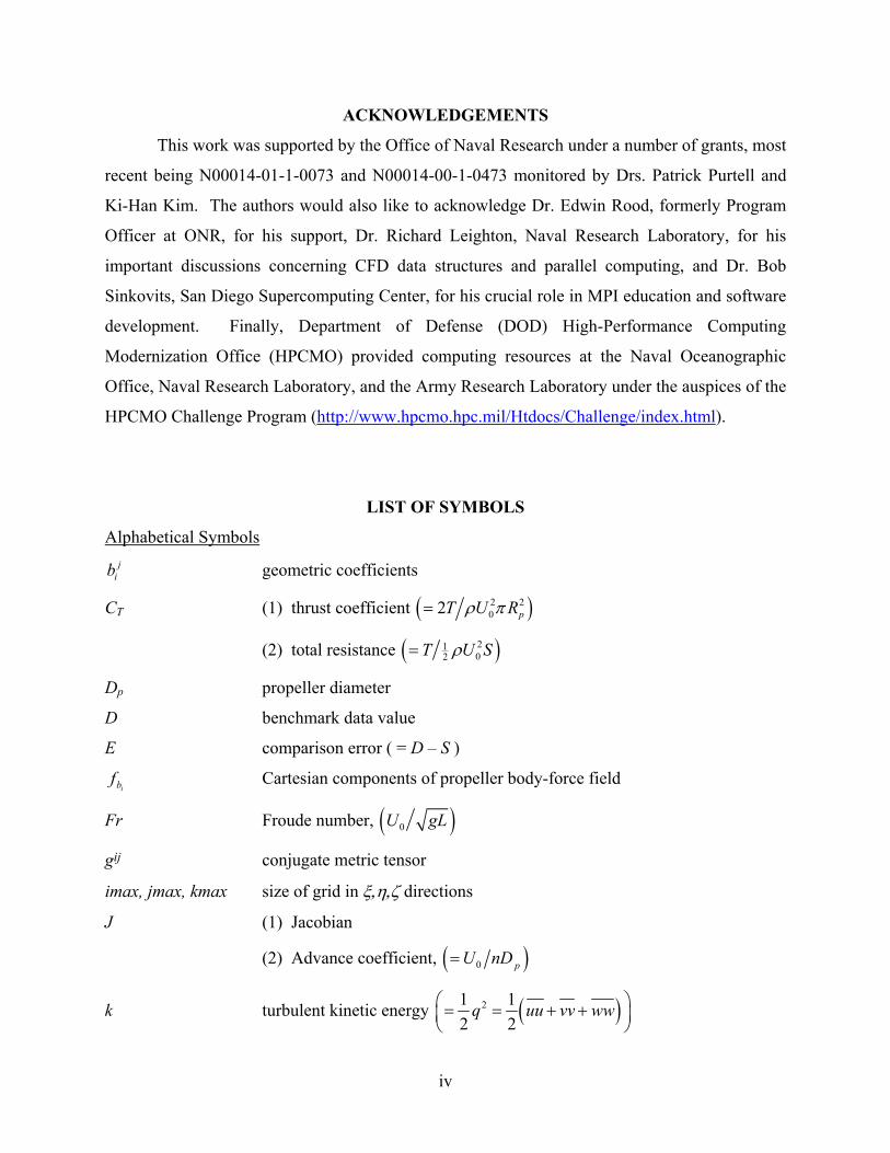
ACKNOWLEDGEMENTS

This work was supported by the Office of Naval Research under a number of grants, most

recent being N00014-01-1-0073 and N00014-00-1-0473 monitored by Drs. Patrick Purtell and

Ki-Han Kim. The authors would also like to acknowledge Dr. Edwin Rood, formerly Program

Officer at ONR, for his support, Dr. Richard Leighton, Naval Research Laboratory, for his

important discussions concerning CFD data structures and parallel computing, and Dr. Bob

Sinkovits, San Diego Supercomputing Center, for his crucial role in MPI education and software

development. Finally, Department of Defense (DOD) High-Performance Computing

Modernization Office (HPCMO) provided computing resources at the Naval Oceanographic

Office, Naval Research Laboratory, and the Army Research Laboratory under the auspices of the

HPCMO Challenge Program (http://www.hpcmo.hpc.mil/Htdocs/Challenge/index.html).

LIST OF SYMBOLS

Alphabetical Symbols

bij geometric coefficients

CT (1) thrust coefficient ( )2 202 pT U Rρ π=

(2) total resistance ( )2102T U Sρ=

Dp propeller diameter

D benchmark data value

E comparison error ( = D – S )

fbi Cartesian components of propeller body-force field

Fr Froude number, ( )0U gL

gij conjugate metric tensor

imax, jmax, kmax size of grid in ξ,η,ζ directions

J (1) Jacobian

(2) Advance coefficient, ( )0 pU nD=

k turbulent kinetic energy ( )21 12 2

q uu vv ww = = + +

v

KT thrust coefficient ( )2 4pT n Dρ=

KQ ` torque coefficient ( )2 5pQ n Dρ=

L characteristic length (ship length at design waterline)

n revolutions per second of propeller

p non-dimensionalized static pressure, ( )( )2o op p Uρ= −

$p piezometric pressure, 2 20

p p zU Frρ

∞ −= +

Re Reynolds number, ( )0U L ν=

Rφ effective Reynolds number

S (1) wetted surface area

(2) simulation value

Sφ, sφ source functions

t time

Ui Velocity components (U,V,W) in Cartesian or cylindrical coordinates

Ui modified contravariant velocity components

$Ui pseudovelocity components

U0 reference velocity (ship speed)

Uτ friction velocity, ( )wτ ρ=

UD experimental uncertainty

USN simulation numerical uncertainty

UV validation uncertainty

Vi contravariant velocity components

u ui j Reynolds stress tensor

xi Cartesian (x,y,z) or cylindrical (x,r,θ) coordinates

y+ wall coordinate ( )U yτ ν=

vi

Greek Symbols

φ velocity components (U,V,W)

κ von Kármán constant

ε turbulent dissipation

ν kinematic viscosity

νt eddy viscosity

ρ fluid density

ω specific dissipation rate

ωx, ωy, ωz angular velocity around x-, y-, and z-axis

τ time in computational domain

τw wall-shear stress

ξi curvilinear coordinates (ξ,η,ζ)

ζ wave elevation

∇ gradient operator

∇2 Laplacian operator

vii

FONT CONVENTIONS

The following conventions are used in this report:

Italic

is used for variables and mathematical symbols

Constant Width

is used for programs and procedures, input variables, and in examples to show the

contents of files or the output from commands. Constant Width Bold

is used in examples to show commands or other text that should be typed literally by the

user. (For example, mpirun -np 1 cfd_ship means to type "mpirun -np 1

cfd_ship" exactly as it appears in the text or the example)

Constant Width Italic

is used in examples to show variables for which a context-specific substitution should be

made. (The variable filename, for example, would be replaced by some actual

filename).

%

is the UNIX C shell prompt

1

1. INTRODUCTION

Reynolds-averaged Navier-Stokes (RANS) computational fluid dynamics (CFD) codes

have matured for most disciplines and are rapidly being integrated into the design process such

that the reality of physics-based simulation based design seems imminent. General-purpose

research codes are available for many engineering applications such as aerospace (Meakin and

Wissink, 1999; Bush et al., 1998), ship hydrodynamics (Hyams et al., 2000; Larsson et al.,

2000), and turbomachinery (Chima, 2001; Hall et al., 1999) whereas other applications, such as

automobile and industrial processes, primarily take advantage of commercial codes. Most codes,

especially commercial ones, can handle more than one application. Code development has

evolved from Ph.D. thesis projects to dedicated groups at academic institutes, government and

industry laboratories, and commercial companies. These groups struggle to keep pace with the

requirements of the design community by addressing issues of modeling, numerical methods,

high performance computing (HPC), structured and unstructured grids and grid generation, and

pre and post processing. Other pace setting issues include lack of trained users and consensus on

quality assessment verification and validation (V&V) methodology and procedures.

Present interest is in ship hydrodynamics, which has unique features in comparison to

related applications due large Reynolds number (Re) ≈ 109; small Mach number (incompressible

flow); tanker, cargo/container, and combatant geometries; ballast, motions, maneuvering,

restricted water, and ambient waves operating and environmental conditions; Froude number (Fr)

and free-surface effects (waves, spray, breaking, near-surface turbulence, and boundary-layer

and wake and vortex interactions); and propulsor-body interactions and cavitation. Detailed

physics vary considerably depending on geometry and operating and environmental conditions.

The status of ship hydrodynamics CFD for steady flow design conditions was assessed at

the recent Gothenburg 2000 Workshop on CFD in Ship Hydrodynamics (Larsson et al., 2000).

Twenty groups representing 16 (8 academic and 8 industrial) institutes and 1 commercial CFD

code company from 11 countries submitted results for one or more of three test cases for modern

tanker, container, and surface-combatant hull forms with validation focusing on, respectively,

turbulence modeling and full-scale Re; free-surface effects and propeller-hull interaction; and

free-surface effects. Verification was required for each group for at least one of the test cases

and the V&V approach of Stern et al. (2001) was recommended. Most codes used 2 or more

2

equation turbulence models and had free-surface capability; finite volume or difference and 2nd-

and 3rd-order accurate numerical methods; multi or single block structured grids; and either

pressure Poisson-equation or artificial compressibility formulations. Few codes included

capability for propulsor modeling, unstructured grids, or parallel computing. Most groups

conducted verification for resistance CT and many followed recommended procedures; however,

there were some problems due to solutions far from asymptotic range and lack of experience

with detailed verification procedures, especially for practical applications. Seven codes showed

grid convergence for CT with average number of grid points 1.5M and simulation numerical

uncertainty USN=3.65%. Some groups showed oscillatory convergence and variability between

grid studies, which indicates need for finer grids. Quantitative validation was performed for CT.

The average comparison error was E=5%, which approximately equals the validation uncertainty

UV=5% such that the codes are approximately validated at the 5% level, which interestingly is

also equal to the coefficient of variation for CT. The average experimental uncertainty was

UD=1.6%. Only qualitative validation was performed for point variables. The Reynolds stress

turbulence models performed best, however 2 equation models were also surprisingly good.

Both surface tracking and capturing methods showed good free surface results.

Advancements for off-design problems and unsteady flow, although warranted since

previous CFD Workshop Tokyo (Kodama, 1994), are still relatively rare. For off-design yaw,

steady turn, and shallow water problems, steady flow methods can still be used and have shown

fairly good agreement with data, although issues remain as to resolution of steep and breaking

waves and body and wave-induced vortices (Tahara et al., 1998; Alessandrini and Delhommeau,

1998; Hochbaum, 1999; Di Mascio and Campana, 1999; Ohmori et al., 2000). For unsteady

flow problems, studies are very limited partly due to the fact that not all steady flow methods are

easily extended to unsteady flow. Ohmori (1998) performs simulations of unsteady combined

sway and yaw motions as per captive model testing in towing tanks using planar motion

mechanisms; however, the free-surface is neglected, i.e., simulations are for the so-called double

body zero Froude number problem. Beddhu et al. (1998), Gentaz et al. (1999), and Yeung et al.

(2000) perform simulations for forced motions, and Sato et al. (1999) and Rhee and Stern (2001)

perform simulations for motions in regular head waves. With capability for more practical

geometries and conditions, coupled with continuing improvements in HPC resources, the

3

promise of CFD-based optimization will soon be realized (Tahara et al., 2000; and Dreyer,

2002).

This report provides documentation of code development of CFDSHIP-IOWA, which is a

general-purpose parallel unsteady RANS ship hydrodynamics code. It is intended for use both in

research and design at universities, and industrial and governmental laboratories. The approach

includes 2-equation turbulence, free-surface tracking, and body-force propulsor modeling;

structured overset-grid, higher-order finite-difference, and pressure-implicit split-operator

(PISO), numerical methods; parallel and portable high performance computing (HPC); and open

source, commented, and modular programming with revision control; and web site distribution

(http://www.iihr.uiowa.edu/~cfdship). The current version of CFDSHIP-IOWA has benefited

from predecessor thesis codes (Tahara and Stern, 1996; Rhee and Stern 2001), but as a complete

package represents significantly improved modeling, numerical methods, HPC, and overall code

development effort. Current version is primarily intended for steady and unsteady resistance and

propulsion simulations, including option of with or without free surface and body force modeling

or complete propulsor. Forthcoming versions will include capability for body motions enabling

steady and unsteady ship motions and maneuvering simulations.

Code development was done over period of last 10 years during which time earlier

versions were released (Paterson et al., 1998; Wilson et al., 1998) and used as intended for

numerous applications including: turbulence modeling (Walker, 2000; Gill, 2000); two phase

flow modeling (Larreteguy, et al., 1998); wave-induced separation (Kandysami, 2001);

maneuvering (Simonsen and Stern, 2003); surface-ship motions (Weymouth et al., 2003; Wilson

and Stern, 2002); optimization (Tahara et al., 2000); propulsor flows (Kim et al., 2003; Chen,

2000); and preliminary industrial design of DD21, i.e., 21st century US Navy destroyer, through

recent ONR Accelerated Hydrodynamics program. Also, simulations for naval surface

combatant were included at Gothenburg 2000 Workshop. Levels of verification and validation

and overall code performance demonstrated that CFDSHIP-IOWA was among the best codes for

the combatant test case (Wilson et al., 2000).

The report provides documentation of the modeling, numerical methods, and code

architecture for CFDSHIP-IOWA v3.03. An example simulation is presented to demonstrate

capabilities and concluding remarks are provided. This report and a suite of example problems

can be found on the CFDSHIP-IOWA website http://www.iihr.uiowa.edu/~cfdship.

4

2. CFD PROCESS

Overall philosophy for the CFD process is given in this section as a set of procedures to

guide engineers and scientists through the process of modeling fluid flow problems using a CFD

code. Although some of the elements of the CFD process are relatively straightforward,

development of a comprehensive process is useful for training non-expert CFD users,

establishing confidence in results from CFD codes, assessing risks in the use of CFD results in a

design environment, and streamlining the task of obtaining CFD solutions leading to reduced

manpower requirements. As described in the following paragraphs, the CFD process is

composed of two distinct parts, (i) selection or development of a general-purpose CFD code and

(ii) use of the CFD code for solution of a particular flow problem of interest. In general, the

former occurs only at infrequent intervals when need arises to make large shifts in technology,

whereas the latter must be followed for each simulation.

Development of any general-purpose CFD code has several common elements.

Specifically, formulation of the general initial and boundary value problem (IBVP) which is to

be solved numerically using a CFD code, development of numerical methods for approximate

solution of the IBVP, and documentation of the CFD code. Key issues in the formulation of the

IBVP are in definition of the scope and level of flow description (e.g., RANS, LES, DNS),

selection of governing partial differential equations (PDEs) and physical models for the fluid

flow, and selection of a comprehensive set of initial and boundary conditions required to solve a

wide range of applications. With regard to numerical methods, key issues include discretization

of the continuous modeled PDEs, initial and boundary conditions, development of numerical

algorithms for solution of the discretized modeled equations, and programming and testing the

algorithm in a CFD code. Finally, documentation of the CFD code is required to assist users in

running the code. Additional documentation may be required to assist other users in the

development of new models or numerical methods.

The CFD process for simulation of a fluid flow application is summarized here in six

distinctive phases as shown in Fig. 1. The process is initiated by clearly defining the purpose for

the CFD simulation and the acceptable levels of CFD simulation error and uncertainty (e.g.,

prediction of vehicle drag with validation of uncertainty of 5% over a specified range of

Reynolds numbers). The second step is to formulate the IBVP, which involves definition of the

required governing PDEs, physical models, and initial and boundary conditions for the

5

application of interest. In addition, the flow geometry, domain, and coordinate system are

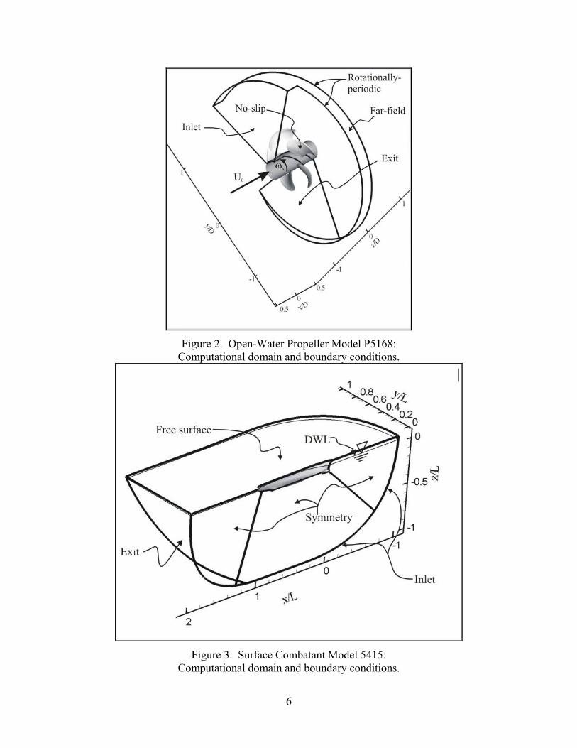
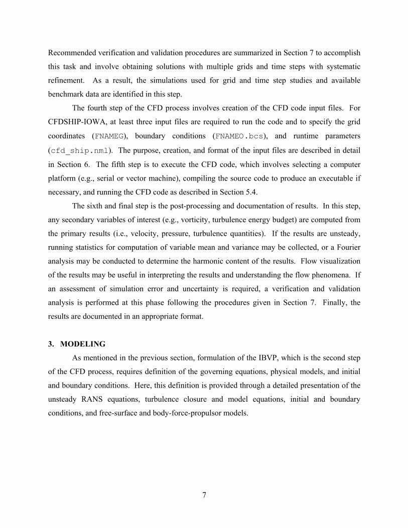
defined in this step. As an aid in later steps, it is often useful to construct sketches, such as those

shown in Figs. 2 and 3, which summarize geometry, domain, coordinate system, and boundary

conditions. It is assumed that the selected CFD code meets the requirements for the

CFD Process 1. Define purpose and required levels for V&V

2. Formulate the IBVP • Define continuous PDEs • Define physical models • Define initial and boundary conditions • Define geometry, domain, coordinate system

3. Plan simulation matrix

4. Create input files • Generate grid(s) • Prescribe boundary conditions • Prescribe initial conditions • Select flow conditions • Select models • Select numerical parameters and post-processing variables

5. Execute CFD code

6. Post-process and document results

Figure 1. CFD Process

particular application as defined in this step or can be modified to do so with an acceptable level

of effort. If further code development is required, issues with source code architecture and

availability become important as discussed in Section 4. These issues may impact whether the

user selects a commercial or research code.

The third step involves planning of the simulation matrix (i.e., number of simulations

required to study desired range of flow conditions). Depending on the purpose of the CFD

simulation and the environment, some or all cases may be selected to estimate simulation error

and uncertainty through comparison of the simulation results with available benchmark data.

6

Figure 2. Open-Water Propeller Model P5168:

Computational domain and boundary conditions.

Figure 3. Surface Combatant Model 5415:

Computational domain and boundary conditions.

7

Recommended verification and validation procedures are summarized in Section 7 to accomplish

this task and involve obtaining solutions with multiple grids and time steps with systematic

refinement. As a result, the simulations used for grid and time step studies and available

benchmark data are identified in this step.

The fourth step of the CFD process involves creation of the CFD code input files. For

CFDSHIP-IOWA, at least three input files are required to run the code and to specify the grid

coordinates (FNAMEG), boundary conditions (FNAMEO.bcs), and runtime parameters

(cfd_ship.nml). The purpose, creation, and format of the input files are described in detail

in Section 6. The fifth step is to execute the CFD code, which involves selecting a computer

platform (e.g., serial or vector machine), compiling the source code to produce an executable if

necessary, and running the CFD code as described in Section 5.4.

The sixth and final step is the post-processing and documentation of results. In this step,

any secondary variables of interest (e.g., vorticity, turbulence energy budget) are computed from

the primary results (i.e., velocity, pressure, turbulence quantities). If the results are unsteady,

running statistics for computation of variable mean and variance may be collected, or a Fourier

analysis may be conducted to determine the harmonic content of the results. Flow visualization

of the results may be useful in interpreting the results and understanding the flow phenomena. If

an assessment of simulation error and uncertainty is required, a verification and validation

analysis is performed at this phase following the procedures given in Section 7. Finally, the

results are documented in an appropriate format.

3. MODELING

As mentioned in the previous section, formulation of the IBVP, which is the second step

of the CFD process, requires definition of the governing equations, physical models, and initial

and boundary conditions. Here, this definition is provided through a detailed presentation of the

unsteady RANS equations, turbulence closure and model equations, initial and boundary

conditions, and free-surface and body-force-propulsor models.

8

3.1. Governing equations

High-fidelity resolution of a certain portion of the frequency spectrum of unsteady flow

physics and resultant fluid forces and moments can be obtained using unsteady RANS. In the

context of a triple decomposition, an instantaneous flow quantity ( , )f tx can be written as

( ) ( ) ( ) ( ) ( )( , ) , , , ,f t f f t f t F x t f t′′ ′ ′= + + = +x x x x x (1)

where ( )f x is the mean, ( , )f t′′ x are the organized, or deterministic, fluctuations, and ( , )f t′ x

are the turbulent, or random, fluctuations. It is assumed that the RANS equations solve for

( , ) ( ) ( , )F t f f t′′= +x x x and that the Reynolds-averaging process is based upon a time interval

large enough to average out ( , )f t′ x but also small enough to capture ( , )f t′′ x . This implies that

the frequencies of ( , )f t′′ x lay sufficiently outside the spectrum of turbulence and the effect of

turbulence upon ( , )F tx can be modeled as Reynolds stresses. This also implies that for unsteady

RANS, all turbulent production and dissipation is subgrid scale.

The code has been formulated to solve the RANS equations in either Cartesian or

cylindrical-polar base coordinate systems. In addition, both systems may be in either absolute

(i.e., earth-fixed inertial) or relative non-inertial (i.e., fixed to a moving body) reference frames.

Available options with corresponding input parameter values are listed in Table 1.

Table 1. Coordinate system options icoord Description Equations solved

1 Cartesian, absolute frame (2) - (3)

2 Cartesian, non-inertial relative frame (13)

3 Cylindrical, absolute frame (4) - (8)

4 Cylindrical, non-inertial relative frame (4) - (7), (14)

For Cartesian coordinates the continuous continuity and momentum equations in

nondimensional tensor form are

0∂

=∂

i

i

Ux

(2)

2

*ˆ 1i

i i ij i j b

j i j j j

U U UpU u u ft x x Re x x x

∂ ∂ ∂∂ ∂+ = − + − +

∂ ∂ ∂ ∂ ∂ ∂ (3)

9

where Ui = (U, V, W) are the Reynolds-averaged velocity components, xi = (x, y, z) are the

independent coordinate directions, 220

ˆρ

∞ −= +

p pp z Fr

U is the piezometric pressure

coefficient, i ju u are the Reynolds stresses which are a two-point correlation of the turbulent

fluctuations ui, *ibf is the non-dimensional body-force vector ( )2

0ρ=ibf L U where

ibf is a force

per unit volume which represents the effect of the propeller, 0=Fr U gL is the Froude

number, and Re = UoL/ν is the Reynolds number. All equations are nondimensionalized by

reference velocity Uo, length L, and density ρ.

For cylindrical-polar coordinates the continuity and momentum equations in

nondimensional vector form are

( )1 1 0rVU W

x r r r θ∂∂ ∂

+ + =∂ ∂ ∂

(4)

2 *ˆ 1 1 1ib

DU p U uu uv uw fDt x Re x r r θ ρ

∂ ∂ ∂ ∂ = − + ∇ + − − − + ∂ ∂ ∂ ∂ (5)

( )

22

2 2

*

ˆ 1 2

1 1 1ib

DV W p W VVDt r r Re r r

uv vv vw vv ww fx r r r

θ

θ ρ

∂ ∂ − = − + ∇ − − ∂ ∂ ∂ ∂ ∂ + − − − − − + ∂ ∂ ∂

(6)

( )

22 2

*

ˆ1 1 2

1 2 1ib

DW VW p V WWDt r r Re r r

uw vw ww vw fx r r r

θ θ

θ ρ

∂ ∂ + = − + ∇ + − ∂ ∂ ∂ ∂ ∂ + − − − − + ∂ ∂ ∂

(7)

where Ui = (U, V, W) are the velocity components in the axial, radial, and circumferential (x,r,θ)

directions and the operators D/Dt and 2∇ are defined as

2 2 2

22 2 2 2

1 1

D WU VDt t x r r

x r r r r

θ

θ

∂ ∂ ∂ ∂= + + +

∂ ∂ ∂ ∂∂ ∂ ∂ ∂

∇ = + + +∂ ∂ ∂ ∂

(8)

In the absolute frame, body motions are resolved by time-dependent grid motions, which,

as will be explained in section 3, are accounted for in the transformation from physical to

10

computational coordinates. An obvious consequence of moving-body simulations in the absolute

frame is that, except for the simple cases of inertial motions such as steady translation, they are

inherently unsteady.

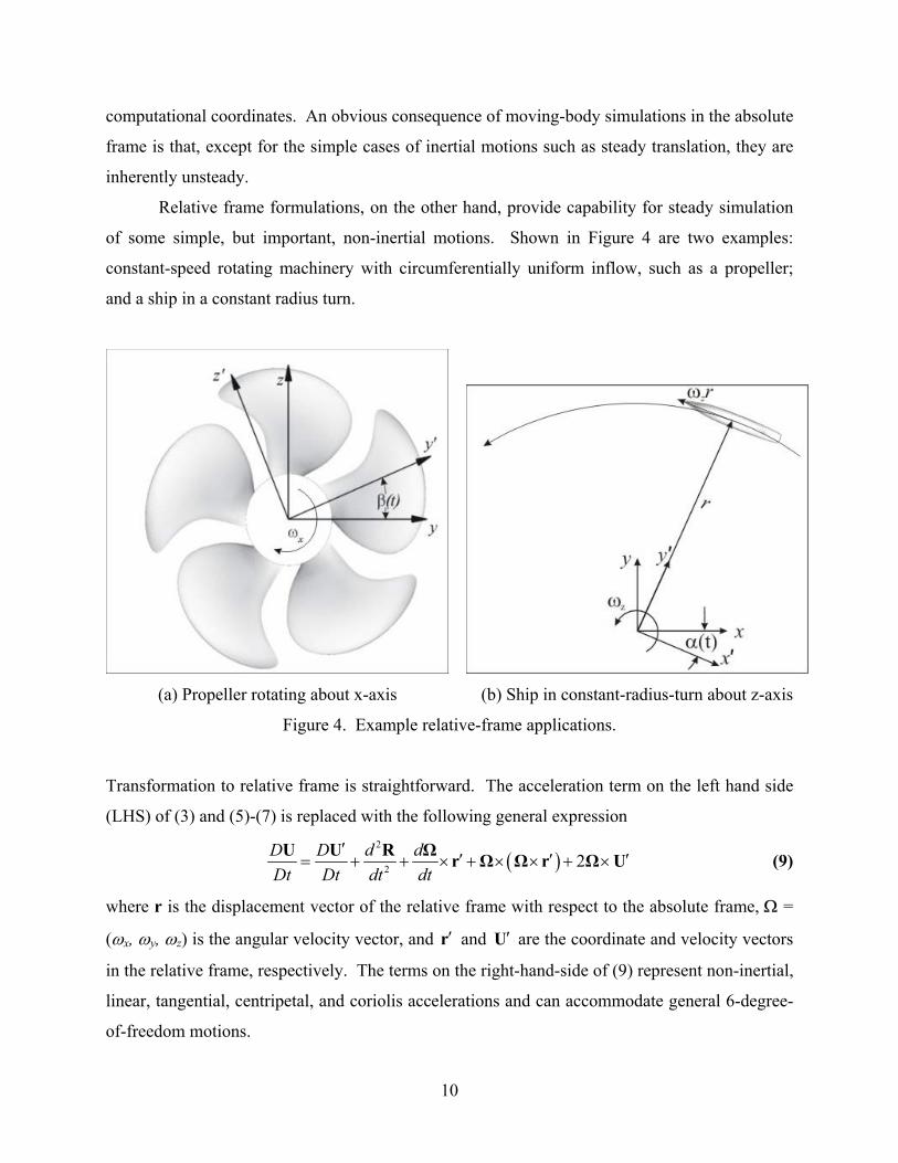
Relative frame formulations, on the other hand, provide capability for steady simulation

of some simple, but important, non-inertial motions. Shown in Figure 4 are two examples:

constant-speed rotating machinery with circumferentially uniform inflow, such as a propeller;

and a ship in a constant radius turn.

(a) Propeller rotating about x-axis (b) Ship in constant-radius-turn about z-axis

Figure 4. Example relative-frame applications.

Transformation to relative frame is straightforward. The acceleration term on the left hand side

(LHS) of (3) and (5)-(7) is replaced with the following general expression

( )2

2 2D D d dDt Dt dt dt

′′ ′ ′= + + × + × × + ×

U U R Ω r Ω Ω r Ω U (9)

where r is the displacement vector of the relative frame with respect to the absolute frame, Ω =

(ωx, ωy, ωz) is the angular velocity vector, and ′r and ′U are the coordinate and velocity vectors

in the relative frame, respectively. The terms on the right-hand-side of (9) represent non-inertial,

linear, tangential, centripetal, and coriolis accelerations and can accommodate general 6-degree-

of-freedom motions.

11

Currently, however, relative-frame motion in Cartesian coordinates is restricted to steady

rotation about either the x- or z-axes. For these simple cases, (9) reduces to the following

2

2 2

2

22 2

2

z z

x x z z

x x

y VD D y W x UDt Dt

z V

ω ωω ω ω ω

ω ω

′ ′ − −′ ′ ′ ′ ′= + − − − +

′ ′− +

U U (10)

where ( ), ,x y z′ ′ ′ and ( ), ,U V W′ ′ ′ are the coordinates and velocity components in the relative

frame. As shown in Figure 4, the relationship between frames is a function of time, defined by

the angle β(t) or α(t). In cylindrical coordinates, motion is restricted to steady rotation about the

x-axis, which reduces (9) to

2

02

2x x

x

D D r WDt Dt

Vω ω

ω

′ ′ ′= + − −

′+

U U (11)

In addition to modifying the acceleration terms, the initial and boundary conditions must be

transformed into relative frame. This results in a large solid-body rotation of the free-stream

velocity and is the usual approach to formulating relative-frame codes (e.g., Chen, 2000).

An alternative approach is used here which has the benefits of removing the solid-body

rotation, moving most of the non-inertial terms from the source-term on the RHS to the

convective terms on the LHS of (3) and (5)-(7), and simplifying calculation of vorticity and wall-

shear stress, such that the same algorithms may be used for either reference frame. To derive

such a system of equations, a new relative-frame velocity vector ( ), ,U V W′′ ′′ ′′ is defined with the

solid-body rotation removed. In Cartesian coordinates

z

x z

x

U U yV V z xW W y

ωω ω

ω

′′ ′ − ′′ ′= + − + ′′ ′ +

(12)

Rearranging (12) for ( ), ,U V W′ ′ ′ , substituting into (2), (3), and (10), and collecting terms

provides RANS equations in terms of ( ), ,U V W′′ ′′ ′′

12

( ) ( ) ( )

( ) ( ) ( )

2*

2

0

ˆ 1

ˆ 1

i

z x z x

j b zj j j

z x z x

U V Wx y z

U U U UU y U z x U yt x y z

p U uu f Vx Re x x x

V V V VU y U z x U yt x y z

py Re

ω ω ω ω

ω

ω ω ω ω

′′ ′′ ′′∂ ∂ ∂+ + =

′ ′ ′∂ ∂ ∂′′ ′′ ′′ ′′∂ ∂ ∂ ∂′′ ′ ′′ ′ ′ ′′ ′+ − + − + + −

′ ′ ′∂ ∂ ∂ ∂

′′∂ ∂ ∂= − + − + −

′ ′∂ ∂ ∂ ∂

′′ ′′ ′′ ′′∂ ∂ ∂ ∂′′ ′ ′′ ′ ′ ′′ ′+ − + − + + −′ ′ ′∂ ∂ ∂ ∂

′′∂ ∂= − +

′∂

( ) ( ) ( )

*

2*ˆ 1

i

i

j b x zj j j

z x z x

j b xj j j

V vu f W Ux x x

W W W WU y U z x U yt x y z

p W wu f Vz Re x x x

ω ω

ω ω ω ω

ω

∂− + − +

′ ′ ′∂ ∂ ∂

′′ ′′ ′′ ′′∂ ∂ ∂ ∂′′ ′ ′′ ′ ′ ′′ ′+ − + − + + −′ ′ ′∂ ∂ ∂ ∂

′′∂ ∂ ∂= − + − + +

′ ′ ′ ′∂ ∂ ∂ ∂

(13)

As a result, all of the centripetal and half the Coriolis terms have been effectively moved to the

LHS of (13) in the form of modified convective velocities. For cylindrical coordinates, similar

transformation may be performed. However, in this case, all of the non-inertial terms are moved

to the LHS such that the governing equations are exactly the same as (4)-(7) with

( ) ( ), , , ,U V W U V W′′ ′′ ′′= , except for the following modification of the substantial derivative

( )xW rD U VDt t x r r

ωθ

′′ ′−∂ ∂ ∂ ∂′′ ′′= + + +′ ′ ′ ′∂ ∂ ∂ ∂

(14)

It is noted that this approach is essentially the same as the Arbitrary Lagrangian Eulerian (ALE)

methods (Hirt et al., 1974) wherein the convective velocity is defined as the difference between

fluid particle velocity and the mesh velocity.

Although there are numerous subroutines that have coordinate-system dependent logic

(e.g., boundary condition formulation, calculation of wall-proximity functions and wall-shear

stress, and coordinate transformation including grid-velocity terms), users only are required to

specify consistent coordinate system (icoord), flow conditions (agvx, agvy, agvz),

and boundary conditions, the latter of which are discussed in Section 4.6.

13

3.2. Turbulence

CFDSHIP-IOWA is designed to use a linear closure model where the Reynolds stresses

are directly related to the mean rate-of-strain through an isotropic eddy viscosity νt. In Cartesian

coordinates, it is written as

23

jii j t ij

j i

UUu u kx x

ν δ ∂∂

− = + − ∂ ∂ (15)

where δij is the Kronecker delta and ( )21 12 2

k q uu vv ww= = + + is the turbulent kinetic energy.

In cylindrical coordinates,

23

1 23

1 23

2

2

2 2

t ij

t ij

t ij

t

t

t

U Vuv kr x

U Wuw kr x

V W Wvw kr r r

Uuux

VvvrW Vww

r r

ν δ

ν δθ

ν δθ

ν

ν

νθ

∂ ∂ − = + − ∂ ∂ ∂ ∂ − = + − ∂ ∂ ∂ ∂ − = + − − ∂ ∂ ∂ − = ∂ ∂ − = ∂

∂ − = + ∂

(16)

For unsteady flow, equations (15) and (16) are quasi-steady relationships where it is assumed

that − i ju u responds instantaneously to the mean rate of strain.

Substituting (15) for the Reynolds-stress term in (3), the momentum equations in

Cartesian coordinates become

21

i

i

ji i i t ij b

j i U j j j j i

UU U U UPU ft x x R x x x x x

ν ∂∂ ∂ ∂ ∂ ∂∂+ = − + + + + ∂ ∂ ∂ ∂ ∂ ∂ ∂ ∂

(17)

where

2ˆ3

= +P p k (18)

14

1 1

i

tUR Re

ν= + (19)

The same can be done for cylindrical coordinates where (16) is substituted into (5),(6), and (7)

2

*

1

1 1 12

i

i

U

t t tb

DU P UDt x R

U U V U W fx x r r x r r xν ν ν

θ θ ρ

∂= − + ∇

∂

∂ ∂ ∂ ∂ ∂ ∂ ∂ ∂ + + + + + + ∂ ∂ ∂ ∂ ∂ ∂ ∂ ∂

(20)

22 2

2 2

*

1 22

1 1 12

i

i

U

t t tb

DV W P W VW r VDt r r R r r

U V V V W W fx r x r r r r r r

ω ωθ

ν ν νθ θ ρ

∂ ∂ − − − = − + ∇ − − ∂ ∂

∂ ∂ ∂ ∂ ∂ ∂ ∂ ∂ + + + + + − + ∂ ∂ ∂ ∂ ∂ ∂ ∂ ∂

(21)

22 2

*

1 1 22

1 1 1 2 2 1i

i

U

t t tb

DW VW P V WV WDt r r R r r

U W V W W W V fx r x r r r r r r r

ωθ θ

ν ν νθ θ θ θ ρ

∂ ∂ + + = − + ∇ + − ∂ ∂

∂ ∂ ∂ ∂ ∂ ∂ ∂ ∂ + + + + − + + + ∂ ∂ ∂ ∂ ∂ ∂ ∂ ∂

(22)

In CFDSHIP-IOWA, eddy viscosity can be calculated using one of two models: Baldwin-

Lomax or the blended k-ω/k-ε (BKW), including an option for shear-stress transport (SST)

model (Menter, 1994). The turbulence model and options are selected using the input parameters

itm and itm_switch as described in Section 6.

For the Baldwin Lomax model (itm=1), details have previously been documented in

Stern et al. (1996). However, as illustrated in Paterson and Sinkovits (1999), care must be

exercised when using BL for geometries with multiple no-slip surfaces and multi-block grid

systems since the turbulent length scale is calculated as a weighted average based upon the wall

distance y+ to each no-slip surface in a given block. Since a search process through all blocks is

not performed, the length scale may be incorrect given certain blocking topologies. Therefore,

BL is not recommended for general application to complex geometries and/or grid systems.

The BKW model (itm=2) has proven to be robust, applicable to complex geometries and

flows, and fairly accurate. In nearly all circumstances, it is superior to k-ε models, which require

complicated near-wall models that are difficult to implement in a general fashion. The

15

governing equations for the eddy viscosity νt, turbulent kinetic energy k, and the turbulent

specific dissipation rate ω are as follows,

νω

=tk (23)

2

2

1 0

1 0ω ωω

νσ

νω ωσ ω

∂∂ ∂+ − − ∇ + = ∂ ∂ ∂

∂∂ ∂+ − − ∇ + = ∂ ∂ ∂

tj k k

j j k

tj

j j

k kU k st x x R

U st x x R

(24)

where the source terms, effective Reynolds numbers, and turbulence production are defined as

( )

( )

*

21 2

12 1ω ω ω

β ω

ω ωγ βω σω

= − +

∂ ∂= − + + −

∂ ∂

k k

j j

s R G k

ks R G Fk x x

(25)

11 Re

11 Reω

ω

σ ν

σ ν

= +

= +

kk t

t

R

R (26)

( ) ( ) ( )2 22 2 2 22 2 2τ ν∂ = = + + + + + + + + ∂

iij t y x z x z y x y z

j

UG U V U W V W U V W

x (27)

4

21 2 2

202

4500tanh min max ; ;0.09 Re

1max 2 ;10

ω

ω

ω ω

σωδ δ ω δ

ωσω

−

= ∂ ∂

= ∂ ∂

k

kj j

kkFCD

kCDx x

(28)

The blending function F1 was designed to be 1 in the sublayer and logarithmic regions of

boundary layers and gradually switch to zero in the wake region to take advantage of the

strengths of the k-ω and k-ε models, i.e., k-ω does not require near-wall damping functions and

uses simple Dirichlet boundary conditions and the k-ε does not exhibit sensitivity to the level of

free-stream turbulence as does the k-ω model. The distance to the nearest no-slip surface δ is

required for calculation of F1 and the model constants are calculated locally as a weighted

16

average, i.e., ( )1 1 1 21φ φ φ= + −F F where φ1 are the standard k-ω model and φ2 are the

transformed k-ε model constants in Table 2.

Table 2. Blended k-ω/k-ε model constants.

φ φ1 φ2 φ1, SST

σk 0.5 1.0 0.85

σω 0.5 0.856 0.5

β 0.075 0.0828 0.075

β∗ 0.09 0.09 0.09

κ 0.41 0.41 0.41

γ 0.0553 0.04403 0.0553

In addition to the standard BKW model, a SST model (Menter, 1994) is included as a user

specified option. The SST model accounts for transport of the principal turbulent stresses and

has shown improved results for flows with adverse pressure gradients. The SST model is

identical to the standard model except for a change in σk as shown in Table 2 and the definition

of eddy viscosity

( )2

2

2 2

0.31max 0.31 ,

2 500tanh max ,0.09

νω

νω ω

=Ω

=

tk

F

kFy y

(29)

where Ω is the absolute value of the vorticity, and y is the distance to the nearest wall. This

effectively reduces eddy viscosity in regions of high off-body vorticity such as that found in

separated flow or in a tip vortex.

3.3. Initial and Boundary Conditions

Formulation of an IBVP requires mathematical derivation of the initial and boundary

conditions for each dependent variable and for each type of condition that is to be simulated.

Complete presentation of the available palette of conditions and underlying numerics in

CFDSHIP-IOWA is deferred until Sections 4.5 and 4.6. Here, a brief discussion of the initial

and boundary condition modeling is provided.

17

Since CFDSHIP-IOWA can be run in two different modes, i.e., steady (time-asymptotic)

and unsteady (time-accurate), the initial conditions serve two purposes. For steady-flow

simulations, the initial conditions provide the zeroth iteration to an iterative scheme and can be

fairly crude. Usually, out of convenience, free-stream conditions are used throughout the

domain. For unsteady flow, on the other hand, the initial conditions serve as the solution at

time=0.0 and should therefore satisfy the governing equations at this time. General specification

for arbitrary geometries and conditions is nearly impossible; therefore, the available initial

condition corresponds to a start from rest (i.e., U = V = W = P = 0.0, k = kfst, ω = ωfst) with a

cubic polynomial acceleration to ship speed. Details of numerical implementation are provided

in Section 4.5.

As with most CFD codes, there are numerous BC types which, for convenience, can be

grouped into domain truncation boundaries, physical boundaries, and computational boundaries.

Physical BC’s are due to solid surfaces or water-air free surface, the latter of which is described

in the next section. For external-flow hydrodynamics, an infinite unbounded fluid often

represents the physical domain. This requires that the computational domain be truncated to a

size that can be economically filled with grid points, but has no influence on the computed

solution. Computational boundaries are due to grid topology, modeling assumptions, and multi-

block domain decomposition. Available options in CFDSHIP-IOWA are listed in Table 7 and

will be discussed in more complete detail in Section 4.6.

3.4. Free-surface

CFDSHIP-IOWA uses a surface tracking approach for modeling the free surface. The

kinematic free-surface boundary condition (KFSBC) is used to compute the evolution of the free

surface, while the dynamic free-surface boundary condition (DFSBC) provides boundary

conditions for velocity and pressure. Considering the KFSBC, the requirement that the wave

elevation ζ be a stream surface is satisfied by the condition

( ) 0D z

Dtζ −

= (30)

Expanding equation (30) gives a continuous 2D hyperbolic PDE for ζ

0U V Wt x y

∂ζ ∂ζ ∂ζ∂ ∂ ∂

+ + − = (31)

18

At the intersection of free- and no-slip surfaces (i.e., the contact line), equation (31) becomes

singular when the contact line is in motion but the fluid velocity is zero due to the viscous no-slip

boundary condition. This problem is overcome through the use of an approximate contact line

model where a small near-wall region is “blanked out” when solving equation (31) and the

solution in this region is linearly extrapolated from the interior of the domain. The numerical

method for solution of the KFSBC given by equation (31) is presented in Section 4.4.

The DFSBC requires that the normal and tangential stresses are continuous across the

free-surface

*ij j ij jn nτ τ= (32)

where nj is the unit normal vector to the free surface and τij

( )1Reij i j j i i jp U x U x u uδ ∂ ∂ ∂ ∂− = − + + − and τij* are the fluid- and external-stress tensors,

respectively. Although not included in this presentation, the effects of air and surface tension

can be included through the external-stress tensor τij*. The following approximations were used

to obtain free-surface boundary conditions from equation (32): (i) the external stress and surface

tension are assumed zero so that 0ij jnτ = ; and (ii) the gradients of the free surface and normal

velocity in the tangential directions are assumed small (i.e., 0xζ∂ ∂ , 0yζ∂ ∂ , 0W x∂ ∂ ,

and 0W y∂ ∂ ). Under these assumptions, expansion of equation (32) gives the following

approximate dynamic boundary conditions for pressure and tangential velocity components

2pFrζ

= (33)

( ),0

U Vz

∂∂

= (34)

Lastly, a zero-gradient condition is used for W, which is consistent with the approximations

employed for the dynamic condition

0Wz

∂∂

= (35)

3.5. Body-force propulsor

The momentum equations (3) include a body-force term ibf , which may be used to model

the effects of a propulsor without resolving the detailed blade flow. There are numerous

19

approaches to calculating ibf including simple prescribed distributions, which recover the total

thrust and torque, to more sophisticated methods which use a propeller performance code in an

interactive fashion with the RANS solver to capture propeller-hull interaction and to distribute

ibf according to the actual blade loading (e.g., Stern et al., 1994). For the latter, custom interface

software must be developed to extract effective wake from RANS solution and to produce ibf

calculated by performance code. This is not provided with CFDSHIP-IOWA, but can be easily

developed by experienced users with access to a propeller performance code.

CFDSHIP-IOWA does, however, include a prescribed axisymmetric body force with

axial and tangential components (Stern et al., 1988). The radial distribution of forces is based

the Hough and Ordway circulation distribution (Hough and Ordway, 1964) which has zero

loading at the root and tip. Therein,

( )

* *

* *

*

1

11θ θ

= −

−=

− +

bx x

bH H

f A r r

r rf AR r R

(36)

where

( ) ( )

( ) ( )( )

( ) ( )( )

*

2 2

2

1

10516 4 3 1

1054 3 1θ π

−=

−

= − + −

=+ −

=+ −

RP RHRH

Y_PROP_CENTER Z_PROP_CENTER

DXPROP RH RH

DXPROP RH RH

Tx

Q

rr

r y z

CA

KA

J

(37)

and where CT and KQ are the thrust and torque coefficients, J is the advance coefficient, RP is the

propeller radius non-dimensionalized by ship length, RH is the hub radius in decimal percent of

RP, and DXPROP is the mean chord length projected into the x-z plane. As derived, these forces

are defined over an "actuator cylinder" with volume defined by RP, RH, and DXPROP, i.e.,

( )( )2 21π −RP RH DXPROP . Integration of the body forces (36) over this analytical volume

exactly recovers the prescribed thrust and torque,

20

22 20 0

23 2 20 0

π

π

θ

ρ θ

ρ θ

=

=

∫ ∫ ∫

∫ ∫ ∫

P s

H p

P s

H p

R x

bxR x

R x

bR x

T L U f rdxd dr

Q L U f r dxd dr (38)

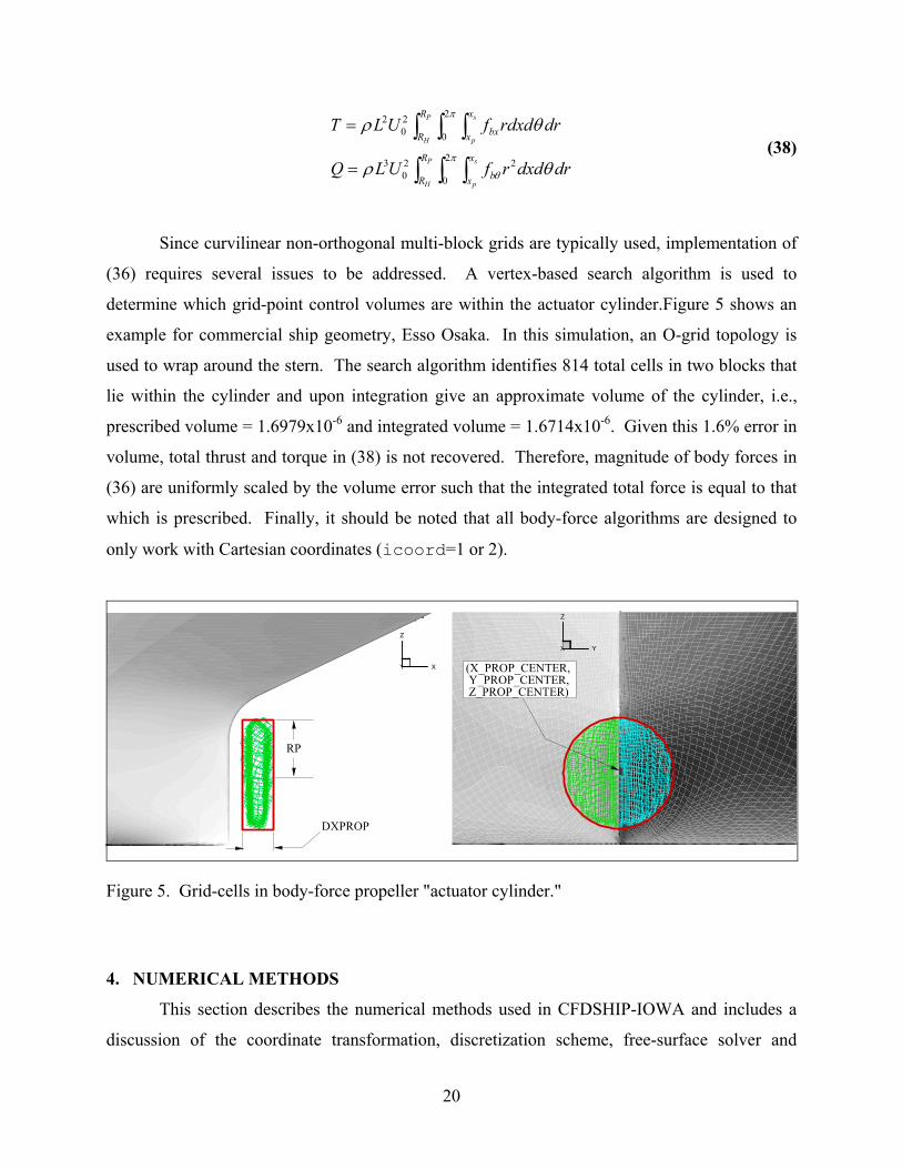
Since curvilinear non-orthogonal multi-block grids are typically used, implementation of

(36) requires several issues to be addressed. A vertex-based search algorithm is used to

determine which grid-point control volumes are within the actuator cylinder.Figure 5 shows an

example for commercial ship geometry, Esso Osaka. In this simulation, an O-grid topology is

used to wrap around the stern. The search algorithm identifies 814 total cells in two blocks that

lie within the cylinder and upon integration give an approximate volume of the cylinder, i.e.,

prescribed volume = 1.6979x10-6 and integrated volume = 1.6714x10-6. Given this 1.6% error in

volume, total thrust and torque in (38) is not recovered. Therefore, magnitude of body forces in

(36) are uniformly scaled by the volume error such that the integrated total force is equal to that

which is prescribed. Finally, it should be noted that all body-force algorithms are designed to

only work with Cartesian coordinates (icoord=1 or 2).

X Y

Z

(X_PROP_CENTER,Y_PROP_CENTER,Z_PROP_CENTER)

Y X

Z

DXPROP

RP

Figure 5. Grid-cells in body-force propeller "actuator cylinder."

4. NUMERICAL METHODS

This section describes the numerical methods used in CFDSHIP-IOWA and includes a

discussion of the coordinate transformation, discretization scheme, free-surface solver and

21

adaptive gridding, RANS solution algorithm and pressure-Poisson equation, initial and boundary

conditions, Chimera overset gridding, and calculation of forces and moments.

4.1. Coordinate transformation

The continuous governing equations are transformed from the physical domain in either

Cartesian (x,y,z,t) or cylindrical-polar (x,r,θ,t) coordinates into the computational domain in non-

orthogonal curvilinear coordinates (ξ, η, ζ, τ). A partial transformation is used in which only the

independent variables are transformed, leaving the velocity components Ui in the base

coordinates. The transformation relations are

( )1 ji ij b q

J ξ∂

∇ ⋅ =∂

q (39)

( ) 1 ji ji

bJ

φφξ

∂∇ =

∂ (40)

2

2 1 ij ij ii j i j iJg g f

Jφ φ φφ

ξ ξ ξ ξ ξ ∂ ∂ ∂ ∂

∇ = = + ∂ ∂ ∂ ∂ ∂ (41)

1 j ii j

xbt J tφ φ φ

τ ξ∂∂ ∂ ∂

= −∂ ∂ ∂ ∂

(42)

where qi represents the components of an arbitrary vector q(xi). The geometric coefficients jib

and ijg , the Jacobian J , and if are functions of coordinates only and are defined for Cartesian

grids as

∂ ∂ε∂ξ ∂ξ

=m n

il lmn j k

x xb (43)

2

1=ij i j

l lg b bJ

(44)

ξ η ζ

ξ η ζ

ξ η ζ

=x x x

J y y yz z z

(45)

( )1 ∂∂ξ

=i ijjf Jg

J (46)

22

where ε lmn is the permutation symbol with lmn cyclic. The grid-velocity terms ixt

∂∂

in (42),

which are used only for unsteady flows in an absolute frame of reference, are calculated directly

using finite difference expressions, as given in the following section.

Using the transformation relations, the continuity (2) and momentum (17) equations are

written as

( ) 01=

∂∂

ij

ij UbJ ξ

(47)

21 1 1 1ν

τ ξ ξ ξ ξ ξ ξ∂ ∂ ∂ ∂ ∂∂

+ = − + + + ∂ ∂ ∂ ∂ ∂ ∂ ∂ i

jk k km k mi i i tU i j i bik k k m k m

eff

UU U UPa b g b b fJ R J J

(48)

where

eff

kj

mtm

jjkj

kU R

fxb

JUb

Ja

i−

∂

∂−

∂∂

−=τξ

ν11 (49)

Note that the convective-term coefficient i

kUa in (49) contains contributions from both the linear

Reynolds-stress closure (15) and the grid velocity (42), the latter of which introduces non-inertial

accelerations due to body motions.

Splitting the viscous term into normal and cross components and rearranging gives the

continuous form of the momentum equations in the computational domain

21 1

i i

k ii ki i iU i Uk i i k

eff

U U U Pa g b sR Jτ ξ ξ ξ ξ

∂ ∂ ∂ ∂+ − = − +

∂ ∂ ∂ ∂ ∂ (50)

2 2 2

12 13 231 2 1 3 2 3

2 1 1i

jk mi i i tU j i bik m

eff

UU U Us g g g b b fR J J

νξ ξ ξ ξ ξ ξ ξ ξ

∂ ∂ ∂ ∂ ∂= + + + + ∂ ∂ ∂ ∂ ∂ ∂ ∂ ∂

(51)

4.2. Discretization scheme

For temporal discretization of equations for k-ω (24), KFSBC (31), and momentum (50),

a general formula for an Euler backward difference is given by

1 21 ( )φ φ φ φτ τ

− −∂= + +

∂ ∆n n n

n m mmwt wt wt (52)

23

where the weights, wtn, wtm, wtmm, determine the order of the difference expression and are given

in Table 3 for the first- and second-order formulations. For steady state and time-accurate

solutions, first-order formulation and second-order formulations are used, respectively, and are

Table 3. Finite-difference weights for temporal discretization. Scheme itemp_order wtn wtm wtmm

1st order 1 1 -1 0

2nd order 2 3/2 -2 1/2

specified using the input variable itemp_order. Eq. (52) is also used to compute grid

velocity terms ixt

∂∂

in Eq. (42) where the general variable φ is replaced with the grid coordinates

xi.

For spatial discretization of equations for k-ω (24), KFSBC (31), geometric coefficients

(43), Jacobian (45), and momentum (50), the convective (or first derivative) terms are discretized

with the following higher-order upwind formula

( ) ( )1 12 2ξ ξ

φ δ φ δ φξ

− +∂= + + −

∂ k k

k k k k k

k

U U U U U (53)

where

2 1 1 2i mm i m i n i p i pp iw w w w wξδ φ φ φ φ φ φ−− − + += + + + + (54)

2 1 1 2i pp i p i n i m i mm iw w w w wξδ φ φ φ φ φ φ+− − + += − − − − − (55)

Six convective schemes are available in CFDSHIP-IOWA and their weighting coefficients are

supplied in Table 4.

Table 4. Finite-difference weights for spatial discretization of convective terms. Scheme ispat_order wmm wm wn wp wpp

1st order upwind 1 0 -1 1 0 0

2nd order central 2 0 -1/2 0 1/2 0

2nd order upwind 3 1/2 -2 3/2 0 0

2nd order upwind biased (Quick) 4 1/8 -7/8 3/8 3/8 0

3rd order upwind biased 5 1/6 -1 1/2 1/3 0

4th order central 6 1/12 -2/3 0 2/3 1/12

24

The user may specify the order of accuracy for the momentum equations and the KFSBC using

the input variable ispat_order, however, 2nd-order upwind is sufficient for most simulations.

For the BKW, equation (24) is discretized, by default, using the same scheme as the momentum

equations. However, order-of-accuracy can be set to a lower-order scheme using namelist

variable itm_spat_order. To maintain stability, it is occasionally necessary to set the

turbulence model discretizaiton to 1st-order upwind. Evaluation of the transformation relations

in equations (43) and (45) is accomplished using the 2nd-order central scheme.

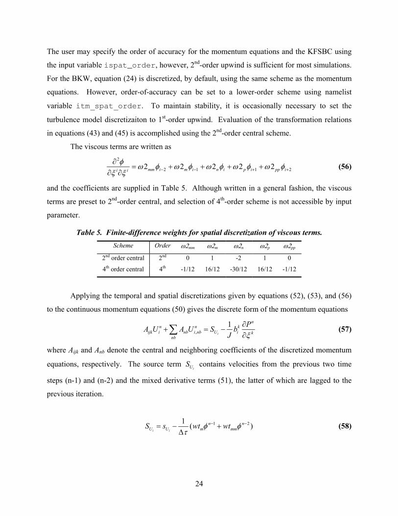
The viscous terms are written as

2

2 1 1 22 2 2 2 2φ ω φ ω φ ω φ ω φ ω φξ ξ − − + +∂

= + + + +∂ ∂ mm i m i n i p i pp ii i (56)

and the coefficients are supplied in Table 5. Although written in a general fashion, the viscous

terms are preset to 2nd-order central, and selection of 4th-order scheme is not accessible by input

parameter.

Table 5. Finite-difference weights for spatial discretization of viscous terms. Scheme Order ω2mm ω2m ω2n ω2p ω2pp

2nd order central 2nd 0 1 -2 1 0

4th order central 4th -1/12 16/12 -30/12 16/12 -1/12

Applying the temporal and spatial discretizations given by equations (52), (53), and (56)

to the continuous momentum equations (50) gives the discrete form of the momentum equations

,1

i

nn n k

ijk i nb i nb U i knb

PA U A U S bJ ξ

∂+ = −

∂∑ (57)

where Aijk and Anb denote the central and neighboring coefficients of the discretized momentum

equations, respectively. The source term iUS contains velocities from the previous two time

steps (n-1) and (n-2) and the mixed derivative terms (51), the latter of which are lagged to the

previous iteration.

1 21 ( )i i

n nU U m mmS s wt wtφ φ

τ− −= − +

∆ (58)

25

4.3. RANS solution algorithm & pressure Poisson equation

The pressure-implicit split-operator (PISO) algorithm for solving the incompressible

Navier-Stokes equations (Issa, 1985) uses a predictor-corrector approach to advance the

momentum equation while enforcing the continuity equation. In the predictor step, the

momentum equation (57) is advanced implicitly using the pressure field from the previous time

step Pn-1

1

* *,

1ξ

−∂+ = −

∂∑n

kijk i nb i nb i i k

nb

PA U A U S bJ

(59)

where superscript ‘*’ is used to denote advancement to an intermediate time level.

In the corrector step, the velocity is updated explicitly

*

** 1ˆξ

∂= −

∂k

i i i kijk

PU U bJA

(60)

using a pressure obtained from a derived Poisson equation and where the psuedo-velocity is

defined as

*,

1ˆ = −

∑i i nb i nbnbijk

U S A UA

(61)

A pressure-Poisson equation is derived by taking the divergence of equation (60)

*

**1 1 1 1ˆξ ξ ξ ξ

∂ ∂ ∂ ∂= − ∂ ∂ ∂ ∂

j j j ki i i i i ij j j k

ijk

Pb U b U b bJ J J JA

(62)

and by realizing that the LHS of equation (62) goes to zero upon convergence

*1 1 ˆ

jkj

i ij k jijk

Jg P b UJ A Jξ ξ ξ

∂ ∂ ∂= ∂ ∂ ∂

(63)

Because a regular, or collocated, grid approach is used, solution of equation (63) requires special

treatment to avoid odd-even decoupling. Fourth-order artificial dissipation is implicitly added by

taking a linear combination of full- and half-cell operators (Sotiropoulos and Abdallah, 1992)

( ) * * * 1ˆ ˆ1 ji ijLP LP NP b U

Jγ γ

ξ∂

− + + =∂

(64)

where L is the full-cell formulation, L is the half-cell formulation, and N is the operator

containing mixed-derivative terms

26

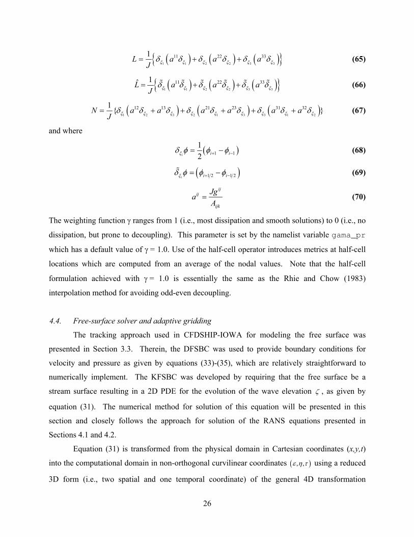
( ) ( ) ( ) 1 1 2 2 3 3

11 22 331ξ ξ ξ ξ ξ ξδ δ δ δ δ δ= + +L a a a

J (65)

( ) ( ) ( ) 1 1 2 2 3 3

11 22 331L a a aJ ξ ξ ξ ξ ξ ξδ δ δ δ δ δ= + +% % % % % % (66)

( ) ( ) ( )1 2 3 2 1 3 3 1 2

12 13 21 23 31 321 ξ ξ ξ ξ ξ ξ ξ ξ ξδ δ δ δ δ δ δ δ δ= + + + + +N a a a a a aJ

(67)

and where

( )1 112ξδ φ φ φ+ −= −

i i i (68)

( )1 2 1 2ξδ φ φ φ+ −= −%i i i (69)

=ij

ij

ijk

JgaA

(70)

The weighting function γ ranges from 1 (i.e., most dissipation and smooth solutions) to 0 (i.e., no

dissipation, but prone to decoupling). This parameter is set by the namelist variable gama_pr

which has a default value of γ = 1.0. Use of the half-cell operator introduces metrics at half-cell

locations which are computed from an average of the nodal values. Note that the half-cell

formulation achieved with γ = 1.0 is essentially the same as the Rhie and Chow (1983)

interpolation method for avoiding odd-even decoupling.

4.4. Free-surface solver and adaptive gridding

The tracking approach used in CFDSHIP-IOWA for modeling the free surface was

presented in Section 3.3. Therein, the DFSBC was used to provide boundary conditions for

velocity and pressure as given by equations (33)-(35), which are relatively straightforward to

numerically implement. The KFSBC was developed by requiring that the free surface be a

stream surface resulting in a 2D PDE for the evolution of the wave elevation ζ , as given by

equation (31). The numerical method for solution of this equation will be presented in this

section and closely follows the approach for solution of the RANS equations presented in

Sections 4.1 and 4.2.

Equation (31) is transformed from the physical domain in Cartesian coordinates (x,y,t)

into the computational domain in non-orthogonal curvilinear coordinates ( ), ,ε η τ using a reduced

3D form (i.e., two spatial and one temporal coordinate) of the general 4D transformation

27

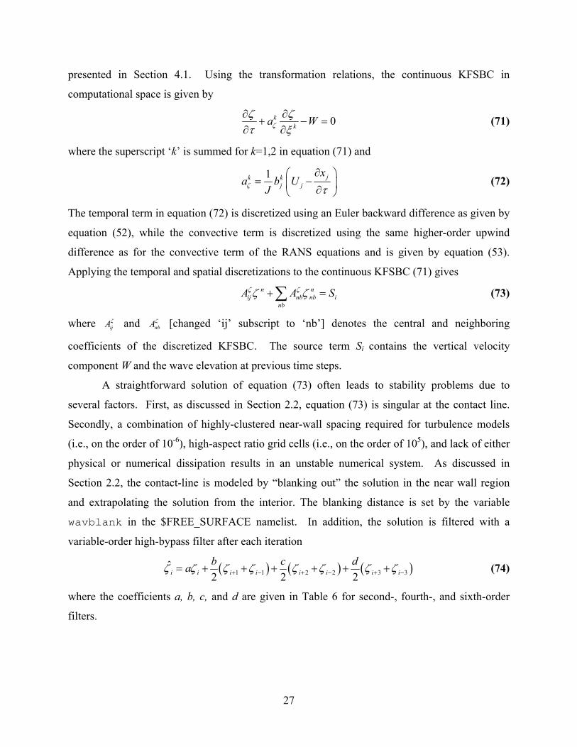
presented in Section 4.1. Using the transformation relations, the continuous KFSBC in

computational space is given by

0kka Wζ

ζ ζτ ξ

∂ ∂+ − =

∂ ∂ (71)

where the superscript ‘k’ is summed for k=1,2 in equation (71) and

1 jk kj j

xa b U

Jζ τ∂

= − ∂ (72)

The temporal term in equation (72) is discretized using an Euler backward difference as given by

equation (52), while the convective term is discretized using the same higher-order upwind

difference as for the convective term of the RANS equations and is given by equation (53).

Applying the temporal and spatial discretizations to the continuous KFSBC (71) gives

n nij nb nb i

nbA A Sζ ζζ ζ+ =∑ (73)

where ijAζ and nbAζ [changed ‘ij’ subscript to ‘nb’] denotes the central and neighboring

coefficients of the discretized KFSBC. The source term Si contains the vertical velocity

component W and the wave elevation at previous time steps.

A straightforward solution of equation (73) often leads to stability problems due to

several factors. First, as discussed in Section 2.2, equation (73) is singular at the contact line.

Secondly, a combination of highly-clustered near-wall spacing required for turbulence models

(i.e., on the order of 10-6), high-aspect ratio grid cells (i.e., on the order of 105), and lack of either

physical or numerical dissipation results in an unstable numerical system. As discussed in

Section 2.2, the contact-line is modeled by “blanking out” the solution in the near wall region

and extrapolating the solution from the interior. The blanking distance is set by the variable

wavblank in the $FREE_SURFACE namelist. In addition, the solution is filtered with a

variable-order high-bypass filter after each iteration

( ) ( ) ( )1 1 2 2 3 3ˆ

2 2 2i i i i i i i ib c daζ ζ ζ ζ ζ ζ ζ ζ+ − + − + −= + + + + + + (74)

where the coefficients a, b, c, and d are given in Table 6 for second-, fourth-, and sixth-order

filters.

28

Table 6. Filter coefficients.

Order a b c d

2nd ½ ½ 0 0

4th 5/8 ½ -1/8 0

6th 11/16 15/32 -3/16 1/32

By transforming the filter from physical to wave number space (Lele, 1992), it can be shown that

the 4th and 6th order filters remove energy at the highest wave number ( k x π∆ ) while leaving

the low wave numbers unchanged. Since the 2nd order filter is overly dissipative, its use should

be avoided. The filter coefficients are specified in the boundary condition file (ifsfilter= 2,

4, or 6) and are default to the 4th-order filter.

The discrete KFSBC given by equation (73) is solved on all block faces identified as a

free-surface boundary using the iterative solvers as described in Section 3.2. After the filtering

operation, the solution is used to conform the volume grid to the new wave elevation through the

use of cubic-spline interpolation in the ζ curvilinear coordinate of the original grid system. This

is equivalent to a “rigid-wire” approach where the grid points slide along the ζ coordinate as

shown in Figure 6.

X Y

ZOrig gridX Y

ZConformed grid

DWL, z/L=0

Figure 6. Dynamic Free-Surface Adaptive Grid.

In general, this approach is fairly robust, but is susceptible to poor grid quality if there is large

difference between the original and conformed grid or if there is severe geometry changes in the

ζ , or girthwise, direction.

29

4.5. Initial conditions

Solution of the IBVP requires initial conditions. For steady-flow simulations, the time-

marching process serves as an iteration loop and the initial conditions provide the zeroth

iteration. Usually, a fairly “poor” initial guess (e.g., free-stream at all grid points, except for no-

slip boundaries) is sufficient such that the algorithm is capable of damping out any initial

transients. For unsteady flow, on the other hand, the initial conditions serve as the solution at

time=0 and initial conditions which do not satisfy governing equations can prevent the

simulation from converging. Excluding custom and/or novel unsteady problems, most

applications can be served by the two initial condition options available in the code.

The first option (mode=0) sets all variables to uniform free stream, i.e., the dependent

variables have the following values U=UINF, V=VINF, W=WINF, p=0, k=kfst=10-7, ω=ωfst=9.0,

and νt,fst=1.1x10-8 where (UINF, VINF, WINF) permits specification of free-stream unit

vector. For steady flow, an impulsive start is used where velocity is set to no-slip values at the

first time step (iteration). In contrast, for unsteady flow, the no-slip boundaries are smoothly

ramped from free-stream values to no-slip values using a cubic polynomial. For time <

time_ramp_end, the no-slip boundaries are set to the following

( )( )( )

3 2

1

1

1

2 3

INF

INF

INF

U U ramp

V V ramp

W W ramp

time timeramp

= −

= −

= −

= − + time_ramp_end time_ramp_end

(75)

This represents a smooth acceleration of the ship from rest and provides initial conditions that

satisfy continuity.

The second option (mode=1) sets initial conditions by reading a restart file. While a

previous simulation typically generates this Fortran binary file, it can also be created by the user

to prescribe either initial conditions or boundary conditions. For the latter, the restart file must

be used in conjunction with boundary condition ibtyp =14 which is described below. Format

of the restart file is described in Appendix A.6.

30

4.6 Boundary conditions

As discussed in Section 2, the CFD Process requires formulation of an IBVP where

boundary conditions (BC) must be specified on all faces of the computational domain. As with

most CFD codes, there are numerous BC types, which for discussion here, can be grouped into

domain truncation boundaries, physical boundaries, and computational boundaries. The

formulation of each BC type is described in detail and guidance provided on when and how each

BC used.

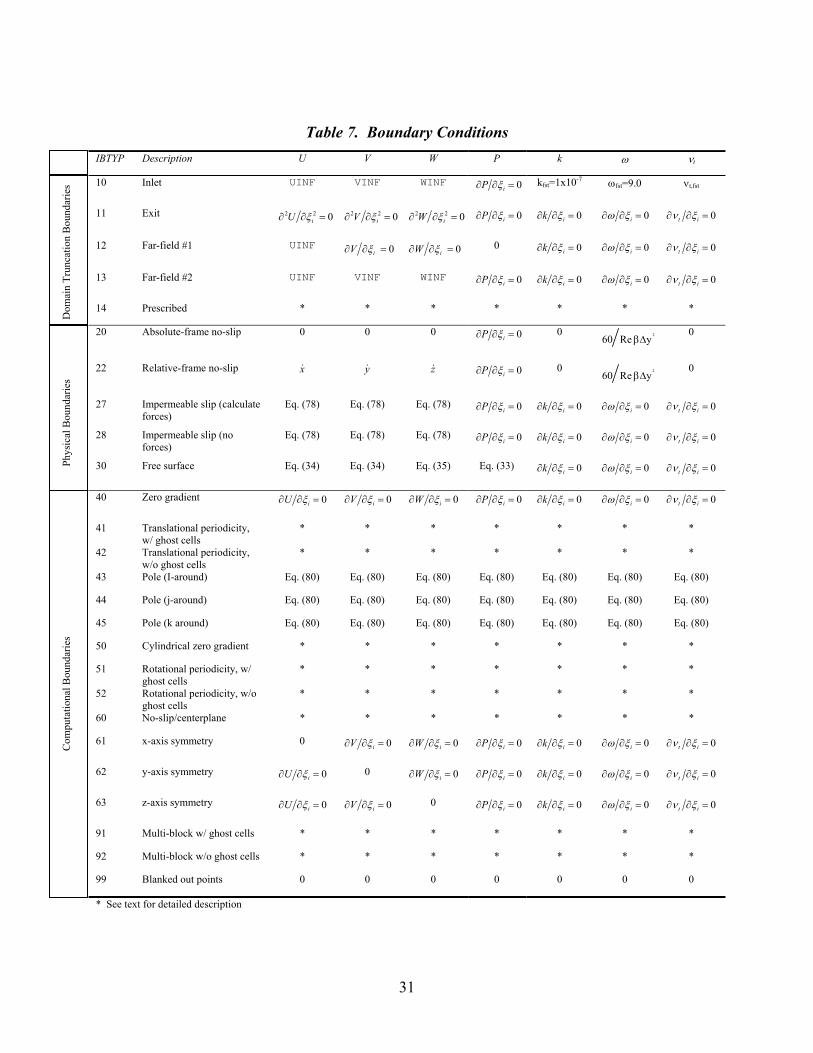
Twenty-six different BC types are available in CFDSHIP-IOWA and are summarized in

Table 7. Each face of each mesh must be specified and can be broken into an arbitrary number

of rectangular patches over which a different boundary condition can be applied. Numerically,

the 26 different conditions consist of combinations of Dirichlet and Neumann boundary

conditions for the nondimensional flow variables U, V, W, p , k, ω and νt. Note that BC for νt

are implemented so that eddy-viscosity gradients in equation (17) can be evaluated near

boundaries without changing finite-difference stencil. Dirichlet conditions are prescribed values

or lagged data from donor regions (i.e., periodic or multiblock). Neumann conditions are

prescribed gradients, which are evaluated using one-sided finite differences. For zero-gradient

conditions, two functions are used in CFDSHIP-IOWA to evaluate first and second derivatives

( )13

a a b= + −zero_fd ibcord (76)

2a b= −zero_sd (77)

where a and b are the values one and two grid points inside the boundary in the ibdir

coordinate direction, respectively. Details unique to each BC type are now described.

31

Table 7. Boundary Conditions IBTYP Description U V W P k ω νt

10 Inlet UINF VINF WINF 0∂ ∂ =iP ξ

kfst=1x10-7 ωfst=9.0 νt,fst

11 Exit 2 2 0∂ ∂ =iU ξ

2 2 0∂ ∂ =iV ξ

2 2 0∂ ∂ =iW ξ

0∂ ∂ =iP ξ

0∂ ∂ =ik ξ 0∂ ∂ =iω ξ

0∂ ∂ =t iν ξ

12 Far-field #1 UINF 0∂ ∂ =iV ξ

0∂ ∂ =iW ξ

0 0∂ ∂ =ik ξ 0∂ ∂ =iω ξ

0∂ ∂ =t iν ξ

13 Far-field #2 UINF VINF WINF 0∂ ∂ =iP ξ

0∂ ∂ =ik ξ 0∂ ∂ =iω ξ

0∂ ∂ =t iν ξ

14 Prescribed * * * * * * *

20 Absolute-frame no-slip 0 0 0 0∂ ∂ =iP ξ

0 2

60 Re yβ∆

0

22 Relative-frame no-slip x& y& z& 0∂ ∂ =iP ξ

0 2

60 Re yβ∆

0

27 Impermeable slip (calculate forces)

Eq. (78) Eq. (78) Eq. (78) 0∂ ∂ =iP ξ

0∂ ∂ =ik ξ 0∂ ∂ =iω ξ

0∂ ∂ =t iν ξ

28 Impermeable slip (no forces)

Eq. (78) Eq. (78) Eq. (78) 0∂ ∂ =iP ξ

0∂ ∂ =ik ξ 0∂ ∂ =iω ξ

0∂ ∂ =t iν ξ

30 Free surface Eq. (34) Eq. (34) Eq. (35) Eq. (33) 0∂ ∂ =ik ξ 0∂ ∂ =iω ξ

0∂ ∂ =t iν ξ

40 Zero gradient 0∂ ∂ =iU ξ

0∂ ∂ =iV ξ

0∂ ∂ =iW ξ

0∂ ∂ =iP ξ

0∂ ∂ =ik ξ 0∂ ∂ =iω ξ

0∂ ∂ =t iν ξ

41 Translational periodicity, w/ ghost cells

* * * * * * *

42 Translational periodicity, w/o ghost cells

* * * * * * *

43 Pole (I-around) Eq. (80) Eq. (80) Eq. (80) Eq. (80) Eq. (80) Eq. (80) Eq. (80)

44 Pole (j-around) Eq. (80) Eq. (80) Eq. (80) Eq. (80) Eq. (80) Eq. (80) Eq. (80)

45 Pole (k around) Eq. (80) Eq. (80) Eq. (80) Eq. (80) Eq. (80) Eq. (80) Eq. (80)

50 Cylindrical zero gradient * * * * * * *

51 Rotational periodicity, w/ ghost cells

* * * * * * *

52 Rotational periodicity, w/o ghost cells

* * * * * * *

60 No-slip/centerplane * * * * * * *

61 x-axis symmetry 0 0∂ ∂ =iV ξ

0∂ ∂ =iW ξ

0∂ ∂ =iP ξ

0∂ ∂ =ik ξ 0∂ ∂ =iω ξ

0∂ ∂ =t iν ξ

62 y-axis symmetry 0∂ ∂ =iU ξ

0 0∂ ∂ =iW ξ

0∂ ∂ =iP ξ

0∂ ∂ =ik ξ 0∂ ∂ =iω ξ

0∂ ∂ =t iν ξ

63 z-axis symmetry 0∂ ∂ =iU ξ

0∂ ∂ =iV ξ

0 0∂ ∂ =iP ξ

0∂ ∂ =ik ξ 0∂ ∂ =iω ξ

0∂ ∂ =t iν ξ

91 Multi-block w/ ghost cells * * * * * * *

92 Multi-block w/o ghost cells * * * * * * *

99 Blanked out points 0 0 0 0 0 0 0

* See text for detailed description

Dom

ain

Trun

catio

n B

ound

arie

s Ph

ysic

al B

ound

arie

s C

ompu

tatio

nal B

ound

arie

s

32

Domain truncation boundaries

For external-flow hydrodynamics, an infinite unbounded fluid often represents the

physical domain. This requires that the computational domain be truncated to a size that can be

economically filled with grid points, but has no influence on the computed solution. Actual

location of boundaries and influence on solution must be evaluated as part of the verification grid

studies which is discussed in Section 7. However, BC types used on truncated domain

boundaries are listed in Table 7 and represent inlet, exit, far-field, and prescribed boundaries.

For the inlet boundary condition (ibtyp=10), the velocity field is set by the input

parameters UINF, VINF, WINF, pressure is zero gradient, and the turbulence is set to the free

stream values 71.0 10 , 9.0fst fstk x ω−= = . The user specified freestream-velocity unit vector

defined by UINF, VINF, WINF provides capability to specify the angle of attack to the

vehicle.

The exit boundary condition, ibtyp = 11 is derived assuming that the boundary is far

downstream such that streamwise viscous effects are zero, i.e., 2 2 2

2 2 2 0i i i

U V Wξ ξ ξ

∂ ∂ ∂= = =

∂ ∂ ∂. This

allows velocity on boundary to be calculated using zero_sd from (77) and all other

variables extrapolated using zero_fd from (76).

There are two far-field conditions, ibtyp=12 and 13. The latter (ibtyp=13) specifies

that velocity field is set by the input parameters UINF, VINF, WINF and pressure and

turbulence variables are zero gradient. This is preferred option, but requires that boundary

location be sufficiently far from vehicle. The former (ibtyp=12), on the other hand, sets the

axial-component of velocity to UINF and pressure to zero while all other variables are assumed

to be zero gradient.

Prescribed boundary condition, ibtyp=14, must be used in combination with a user-

generated restart file, format of which is documented in Appendix A.6. This condition holds all

variables constant to those in the restart file except for pressure, which is calculated assuming a

zero-gradient condition. Typically, this condition is used when specifying either an analytical

(e.g., Blasius flat plate boundary layer) or previously computed flow. An example of the latter

33

may be an isolated propeller blade simulation, where the wake from upstream is computed by a

previous simulation, and used to prescribe inflow boundary conditions.

Physical boundary conditions

Physical BC’s are due to either solid surfaces or water-air free surface. Available options

are listed in Table 7.

There are two no-slip boundary conditions. The first (ibtyp=20) is for surfaces which

are moving with the grid and the second (ibtyp=22) is for surfaces which are moving in the

relative-frame system provided angular velocities (agvx or agvz), which are defined in the

namelist input file cfd_ship.nml.

Impermeable slip boundary conditions are specified using ibtyp=27 and 28, the only

difference being whether or not the specified boundary be included (27) or not (28) in the

calculation of forces and moments. This distinction is useful since impermeable slip boundaries

are often used, for example, to model water-tunnel walls or stream surfaces and it may not be

desired to include the forces on these boundaries in the integration process. The boundary

condition is formulated using contravariant velocity components at one point off the boundary

and by forcing the normal component to be zero. For example, on a j=1 slip surface, the

velocity boundary conditions are

( )( )( )

,1,

,1,

,1,

U i k U x U x U x

V i k U y U y U y

W i k U z U z U z

ξ ξ η η ζ ζ

ξ ξ η η ζ ζ

ξ ξ η η ζ ζ

= + +

= + +

= + +

(78)

where

( ) ( ) ( )( )

( ) ( ) ( )( )

1 1 11 2 3

3 3 31 2 3

1 , 2, , 2, , 2,

0

1 , 2, , 2, , 2,

U U i k b V i k b W i k bJ

U

U U i k b V i k b W i k bJ

ξ

η

ζ

= + +

=

= + +

(79)

and where all other variables are calculated using a zero gradient condition. Similar expressions

can be dervied for i=constant and k=constant surfaces.

As indicated in Table 7, free surface (ibtyp=30) BC have been described earlier in

Section 3.

34

Computational boundaries

Computational boundaries are due to grid topology, modeling assumptions, and multi-

block domain decomposition. Available options in CFDSHIP-IOWA are listed in Table 7 and

include zero-gradient, translational and rotational periodicity, pole singularities, symmetry, and

multi-block boundaries. Each type is now described.

Zero-gradient boundaries (ibtyp=40) assume that all variables have zero gradient

behavior. This condition is provided, but not often used because symmetry conditions, which set

the normal component of velocity to zero, are typically more appropriate.

Translational periodicity, as shown in Figure 8, can be prescribed using either ibtyp =

41 or 42, the difference being that the former uses 2 ghost cells on each boundary to maintain

solver order-of-accuracy and the latter uses a simple weighted average of the adjacent field point

Figure 8. Translational periodic boundary conditions, ibtyp=41 & 42.

values. This boundary condition can be used in either Cartesian or cylindrical coordinates. Note

that all flow variables are assumed periodic.

Pole boundary conditions are based upon simple average of variables one grid point off

the pole in the interior of the domain with three orientations available: i-around (ibtyp=43), j-

around (ibtyp=44), and k-around (ibtyp=45). The orientation specifies the summation

index, e.g., for k-around and ibdir=+2, the U component of velocity on the pole would be

35

( )1( , , ) , 1,1

kbce

k kbcsU i j k U i j k

kbce kbcs =

= +− + ∑ (80)

Rotational periodicity about the x-axis, as shown in Figure 9, can be prescribed using

either ibtyp =51 or 52. As with translational periodicity, the difference between the two is that

the former uses 2 ghost cells on each boundary to maintain solver order-of-accuracy and the

latter uses a simple weighted average of the adjacent field point values. However, in this case,

since the radial and circumferential components are the periodic variables, V and W velocity

components are calculated using the following transformation,

( )1

cos sinsin cos

tan

rV V WV V W

z yθ

θ θθ θ

θ −

= += − +

=

(81)

Note that this boundary condition is restricted to Cartesian grids (icoord=1/2) and with

periodicity about the x-axis only.

Figure 9. Rotational periodic boundary conditions, ibtyp=51 & 52.

Centerplane condition (ibtyp=60) is a boundary condition used for half-domain ship-

hull simulations where part of the boundary is no-slip and part is centerplane, as shown in Figure

10. Demarcation between the no-slip/centerplane is determined by testing the y-coordinate, i.e.,

if 61.0 10y x −≤ then the boundary point is assume to be centerplane, where all variables are

36

Figure 10. Centerplane/no-slip boundary condition, ibtyp=60.

calculated using zero_fd, except for the V-component of velocity which is set to zero,

otherwise the point is treated as no-slip. This boundary condition is typically used to resolve

bow, stern, and/or keel using a staircase resolution (e.g., Stern et al., 1996). It is restricted to

Cartesian grids (icoord=1/2).

Symmetry conditions (ibtyp=61, 62, 63) are available for each coordinate direction.

Formulation is simple: normal component of velocity is set to zero (61, U=0; 62, V=0, 63,

W=0), and all other flow variables are assumed to be zero gradient.

CFDSHIP-IOWA utilizes 2 types of multi-block boundary conditions, pointwise

continuous (i.e., abutted-block interface) and overset (i.e., Chimera), examples of both are shown

in Figure 11.

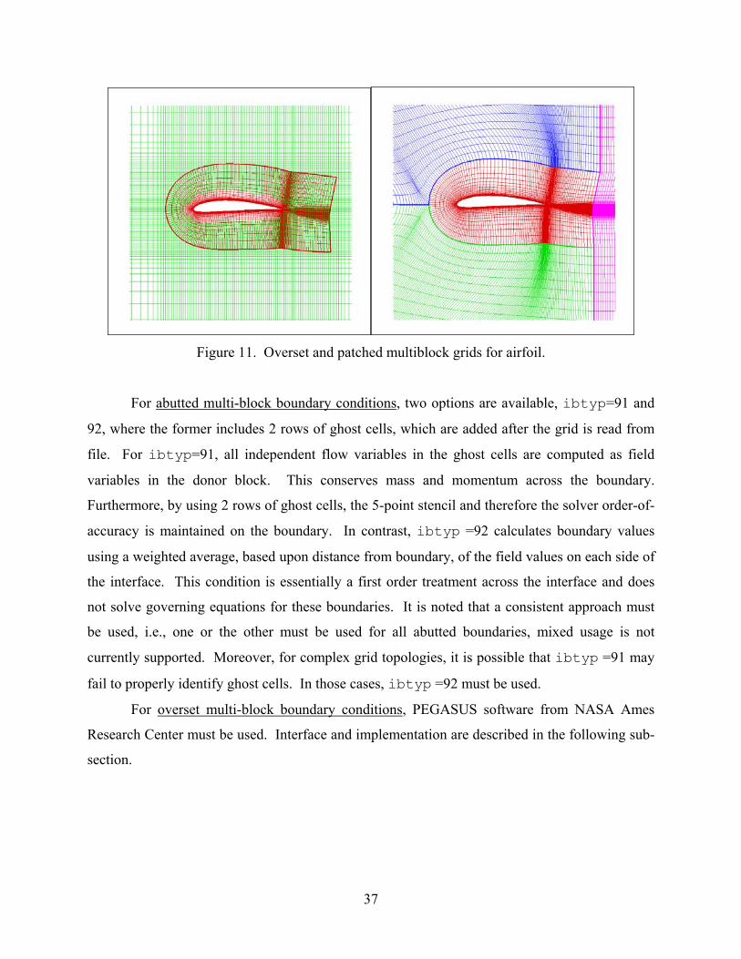
37

Figure 11. Overset and patched multiblock grids for airfoil.

For abutted multi-block boundary conditions, two options are available, ibtyp=91 and

92, where the former includes 2 rows of ghost cells, which are added after the grid is read from

file. For ibtyp=91, all independent flow variables in the ghost cells are computed as field

variables in the donor block. This conserves mass and momentum across the boundary.

Furthermore, by using 2 rows of ghost cells, the 5-point stencil and therefore the solver order-of-

accuracy is maintained on the boundary. In contrast, ibtyp =92 calculates boundary values

using a weighted average, based upon distance from boundary, of the field values on each side of

the interface. This condition is essentially a first order treatment across the interface and does

not solve governing equations for these boundaries. It is noted that a consistent approach must

be used, i.e., one or the other must be used for all abutted boundaries, mixed usage is not

currently supported. Moreover, for complex grid topologies, it is possible that ibtyp =91 may

fail to properly identify ghost cells. In those cases, ibtyp =92 must be used.

For overset multi-block boundary conditions, PEGASUS software from NASA Ames

Research Center must be used. Interface and implementation are described in the following sub-

section.

38

4.7 Chimera overset gridding

Capability for simulations using Chimera-style overset domain decomposition is

accomplished through interface with PEGASUS version 5.1 (Suhs, et al., 2001), which is the

latest version of the PEGASUS series of mesh interpolation codes, originally developed at

NASA Ames Research Center. The main purpose for the development of version 5.1 was to

decrease the number of user inputs required and to allow for easier operation of the code. A

basic description of Chimera methodology is described in the Version 4 manual (Suhs and

Tramel, 1991). It should be noted that PEGASUS is restricted to U.S. institutions and

researchers due to export control regulations. Other options for computation of interpolation

coefficients include CHALMESH (Petersson, 1999), OVERTURE (Quinlan et al., 2002) and

PEGISUE (Denny, 2002).

CFDSHIP-IOWA is designed to use double-fringe hole and outer boundaries and level-2

interpolation. Figure 12 shows an example of an overset grid system for an airfoil to aid in

defining terminology. Comparing Figures 12a and 12b, it can be seen that double-fringe blanks

out 2 layers of cells around the outer and hole boundaries. Both layers are interpolated from the

donor mesh. This permits use of the normal 5-point stencil for all field points and maintains

order of accuracy near boundaries. Single-fringe boundaries, on the other hand, require use of 3-

point stencils for the field points adjacent to hole and outer boundaries, which results in

reduction of the order-of-accuracy. The downside in using a double fringe is that it requires

more mesh points and makes it more difficult to obtain the required overlap between hole

boundaries and outer boundaries.

Figure 12c shows the impact of enabling level-2 interpolation. This is a method where

once the minimum hole has been established; the hole is enlarged to improve the communication

among meshes. In addition, it can be seen that the outer boundary of the foil mesh has been

moved inward. This is accomplished in PEGASUS by comparing relative grid quality between

interpolation and donor meshes so as to reduce mesh disparity, which can severely impact

accuracy. In addition, level-2 interpolation provides capability to create holes with refinement

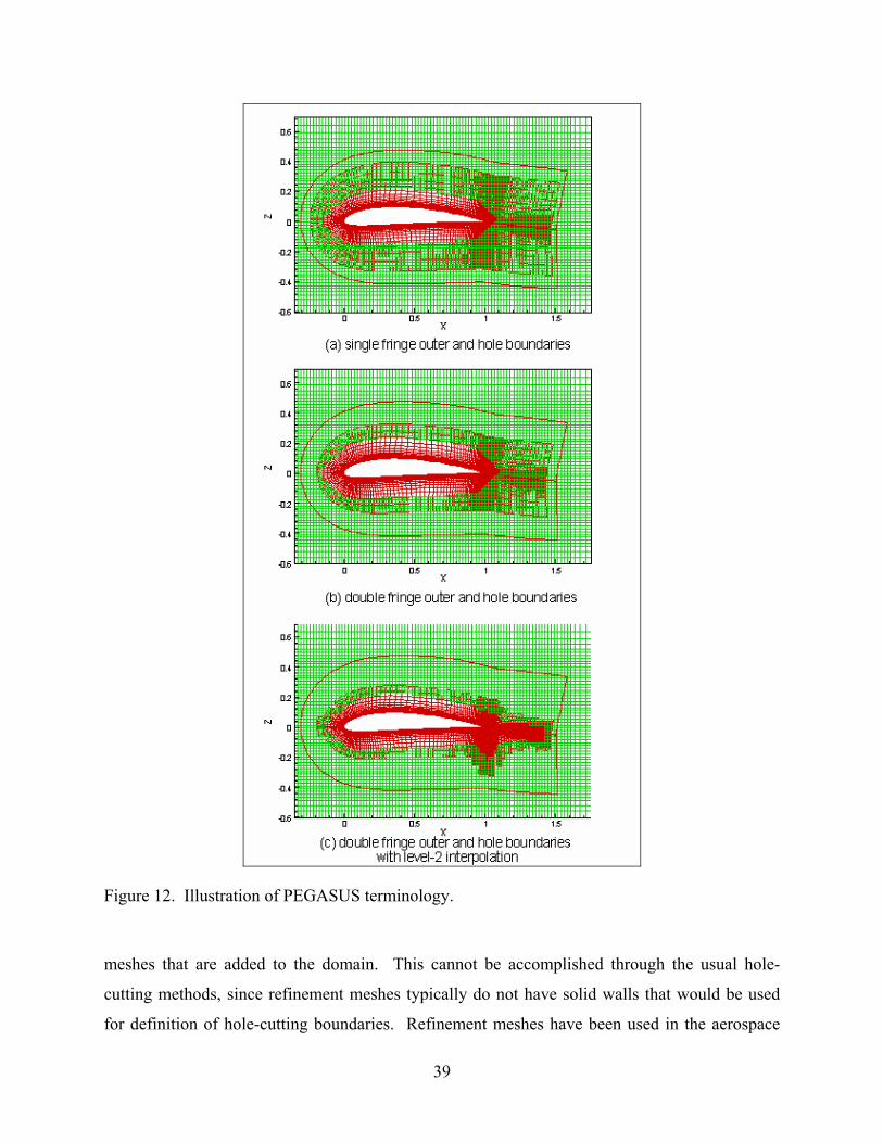
39

Figure 12. Illustration of PEGASUS terminology.

meshes that are added to the domain. This cannot be accomplished through the usual hole-

cutting methods, since refinement meshes typically do not have solid walls that would be used

for definition of hole-cutting boundaries. Refinement meshes have been used in the aerospace

40

community (e.g., Meakin, R., 1999) for flow adaptive refinement within context of structured

flow solvers.

Given a valid PEGASUS interpolation file (i.e., in PEGASUS standard naming

convention, XINTOUT), implementation in CFDSHIP-IOWA is straightforward. This file

should be renamed FNAMEI.xintout since CFDSHIP-IOWA automatically looks for this file

in the execution directory. If it exists, the file is read and a summary is printed in the standard

output. Otherwise, the code continues and prints a notification message that

FNAMEI.xintout does not exist. It should be emphasized that in the boundary condition

input file FNAMEI.bcs Chimera outer boundaries remain unspecified, which for most

problems, greatly simplifies and shortens this input file.

As a summary, Figure 13 provides a flowchart summarizing the overset-grid process.

Further details can be found in the appropriate domain connectivity software, which in this case

is PEGASUS version 5.1.

4.8 Calculation of forces and moments

The fluid forces and moments acting on all solid surfaces are obtained by integration of

the normal and tangential stresses over all no-slip (ibtyp=20,22) and some of the user-

identified slip boundaries (i.e., ibtyp=27). The fluid stress tensor on a no-slip surface is

comprised of components due to pressure and viscous stress

1Re

jiij ij

j i

UUpx x

τ δ ∂∂

= − + + ∂ ∂ (82)

On the solid surfaces, the fluid forces and moments are determined through integration of (82)

ij iSF n dSτ= ∫ (83)

M r F= × (84)

where jn is the unit-vector normal to a ξj-coordinate surface, dSj is the local surface area

element, and r is the position vector

41

( ) ( ) ( )

( ) ( ) ( )

1 2 32 2 2

1 2 2

2 2 2

1 2 2

ˆˆ ˆj j jj

j j j

j j j j i k

b i b j b knb b b

dS b b b d dξ ξ

+ +=

+ +

= + +

(85)

and where (i,j,k) are cyclic. Integration of wetted surface area S and equations (83)-(84) is

accomplished using a cell-centered 2D trapezoidal rule. Calculation of the force is broken down

into contributions from piezometric pressure (cppiezo), hydrostatic pressure (cphydro), which is

valid only for Fr≠0, and viscous shear stress (cf). These contributions, along with the total force

(ctot), are written for each base coordinate direction every iteration. The moments are treated in

a similar fashion.

For overset grid-systems with overlapping surface meshes on solid surfaces, forces and

moments computed by CFDSHIP-IOWA will contain errors due to multiply defined values and

hole boundaries. Special tools must be used to make flow variables single-valued. Currently,

the force and moment computation (FOMOCO) tools from NASA (Chan and Buning, 1996)

represent the only option for performing this task. Two programs make up this toolset, MIXSUR

and OVERINT where the former creates a single-valued mixed surface with triangular zipper

grids and the latter performs integration over this new surface. Unlike the NASA flow solver

OVERFLOW, which reads MIXSUR output as in input file and computes forces and moments

on the fly by calling OVERINT as a subroutine, CFDSHIP-IOWA currently uses these tools in a

stand-alone post-processing fashion. Future versions may more tightly integrate with these tools

or appropriate alternatives.

42

Figure 13. Flowchart of Overset Grid Process

CAD Surface Geometry

Generate surface grids (domains)GRIDGEN

Generate volume grids (blocks) • Near-body : hyperbolic extrusion • Off-body : Cartesian box grids

GRIDGEN

fnamei.bcs fnamei.inp gridname.grd

Compute block-to-block connectivityPegasus v5.1

Convert ASCII grid to unformatted (grid.tmp)

grd-atob

Modify fnamei.inp to create Overflow input file

(over.tmp)

Run peg_setup

Modify peg_in_raw • ORPHFIX=.F. • OFFSET as needed • $HCUT defined as needed

fnamei.xintout

Verify successful domain connectivity achieved • study STD out file • run peg_plot • run peg_diag

Run cfd_ship

43

4.9 Algebraic equation solver

The overall method is fully implicit and there are four locations in the code that require

iterative solvers: momentum predictor step (59); pressure equation (64); turbulence model

equations (24); and KFSBC (31). Currently, a line-ADI scheme with a pentadiagonal solver and

under relaxation is used to solve the algebraic equations. The pentadiagonal solver is modified

to account for hole boundaries

( )

( )

1

1

i i i

i i i

i i i

i i i

i i i

i i i i i

a a IBLANKb b IBLANKc c IBLANKd d IBLANKe e IBLANKf f IBLANK IBLANK φ

==

= −

==

= + −

(86)

where IBLANK is 0 for a hole or fringe point and 1 for a field point, ai, bi, ci, di, ei correspond to

5 diagonals of the pentadiagnoal matrix, fi is the right hand side, and φi corresponds to the flow

variable on the hole or outer boundary fringe.

4.10 Algorithm summary and flowchart

Figures 14 and 15 summarize the algorithmic structure of CFDSHIP-IOWA in

flowcharts, including pre- and post-processing functions, major time marching and iteration

loops, and input and output files.

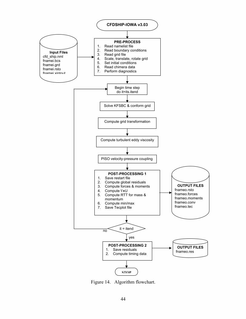
44

Figure 14. Algorithm flowchart.

Begin time step do it=its,itend

Solve KFSBC & conform grid

Compute grid transformation

Compute turbulent eddy viscosity

PISO velocity-pressure coupling

POST-PROCESSING 11. Save restart file 2. Compute global residuals 3. Compute forces & moments 4. Compute ∇•U 5. Compute RTT for mass &

momentum 6. Compute min/max 7. Save Tecplot file

POST-PROCESSING 21. Save residuals 2. Compute timing data

OUTPUT FILESfnameo.rsto fnameo.forces fnameo.moments fnameo.conv fnameo.tec

OUTPUT FILESfnameo.res

CFDSHIP-IOWA v3.03

Input Files cfd_ship.nml fnamei.bcs fnamei.grd fnamei.rsto fnamei xintout

PRE-PROCESS1. Read namelist file 2. Read boundary conditions 3. Read grid file 4. Scale, translate, rotate grid 5. Set initial conditions 6. Read chimera data 7. Perform diagnostics

STOP

it = itend

yes

no

45

Figure 15. Detailed flowchart for PISO velocity-pressure coupling solver

Begin PISO velocity-pressure coupling

Calculate upwind coefficients & source terms of momentum eqns

Setup LHS of momentum penta-diagonal solver

Solve momentum equations

do itv=1,ituvw

Velocity b.c.’s • call chimera_eval • call bc_mb (patched) • call uvwbc

Compute residuals & check convergence

uresid<tol_uvwor

itv = ituvw

yes

no

Calculate coefficients of pressure-Poisson equation

Setup LHS of pressure penta-diagonal solver

Compute psuedo-velocities

do itp=itvpc

Pressure b.c.’s • call chimera_eval • call bc_mb (patched) • call uvwbc

Compute residuals & check convergence

presid < tol_pr or

iter = itpr

yes

no

Compute source term

do iter=itpr

Solve pressure equation

Explicit momentum correction

Velocity b.c.’s • call chimera_eval • call bc_mb (patched) • call uvwbc

Itp = itvpc

yes

no

end PISO

46

5. CODE DEVELOPMENT AND HIGH-PERFORMANCE COMPUTING

Development of CFDSHIP-IOWA has taken place over the past 8 years, a period in

which high-performance computing (HPC) platforms have evolved from Cray YMP vector

processors to the array of architectures found today which includes commercial off-the-shelf

(COTS) Beowulf clusters, SGI scalable distributed-shared non-uniform memory access (NUMA)

architectures, and IBM pipelined superscalar architectures. Developing application codes which

are portable and which are capable of harnessing a given platform’s capability, is a challenging

task. In addition, CFDSHIP-IOWA had to meet other objectives such as supporting student

theses and project research, as well as vertical transition to other universities, industry, and

government labs.

The approach used to meet these objectives has been based upon a flexible data structure,

capability for both serial and parallel computing, adherence to standards such as MPI, modern

programming using Fortran90/95, and interface with existing 3rd-party software for grid

generation and boundary condition specification (GRIDGEN), Chimera overset grid methods

(PEGASUS, Chimera Grid Tools, FOMOCO), and post-processing and visualization

(TECPLOT). It is noted that development has taken place concurrently with several DOD

HPCMO Challenge Projects from 1996 to the present (Rood, 1997; Rood, 1998; Rood, 1999;

Rood, 2000; Kim, 2001). The following sections present an overview of the code and data

structures, parallel computing, portability, and distribution, extraction, compilation and

execution.

5.1. Code and data structures

Code and data structures are critical to successful implementation of scalable parallel

computing and portability. Unfortunately, highly efficient code is often hard to understand by

users. Because CFDSHIP-IOWA was designed to support research and development of new

models, it is well documented with in-code comment statements and the structure at the

subroutine level is based upon 3D index-ordered arrays, which are intuitively easier to

understand in context of structured-grid CFD, and which lends itself naturally to distributed

multi-block computing.

Top-level structure of the code, which is also shown in Figure 14, is as follows

• program cfdship_iowa

47

o pre_process

o free_surface

o grid_transformation

o eddyvs

o piso

o post_process1

o post_process2

In process of writing code, several guidelines were adopted. At top-level, all arrays are dynamic,

1D, and allocatable to fit current grid size. At subroutine level, computation is performed on a

single block; all arrays are 3D and either explicit-shape dummy arrays (both array and

dimensions are in argument list) or automatic arrays (arrays which are not in argument list and

which are created/destroyed upon entry/exit of a given procedure). Index pointers are used to

indicate relative location in 1D array and are defined as follows,

first(1)=1

length(1)=imax(1)*jmax(1)*kmax(1)

last(1)=length(1)

ntot=length(1)

do m=2,nmesh

first(m)=last(m-1)+1

length(m)=imax(m)*jmax(m)*kmax(m)

last(m)=first(m)+length(m)-1

ntot=ntot+length(m)

enddo

(87)

Fortran90 module procedures are used in preference over COMMON blocks to share definitions

and values of data between program units due to ease of code maintenance and data-hiding

capability. To reduce coding errors, IMPLICIT NONE statements are used in all routines.

By design, this approach easily permits parallel multi-block implementation via message-

passing interface (MPI) and the single-program multiple data (SPMD) paradigm. As shown in

the code fragment in Figure 16, serial implementation for a given function performs a DO loop

over each block with the locn pointer set to first(m). This passes each block to the

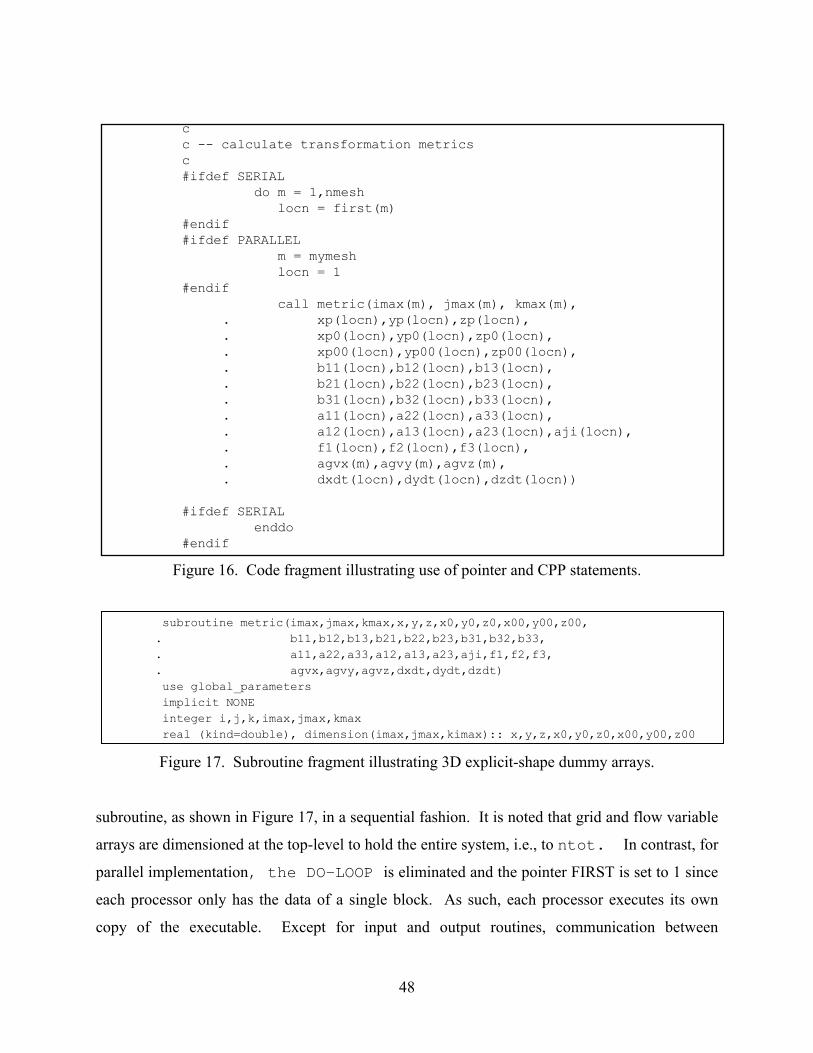
48

cc -- calculate transformation metricsc#ifdef SERIAL do m = 1,nmesh locn = first(m)#endif#ifdef PARALLEL m = mymesh locn = 1#endif call metric(imax(m), jmax(m), kmax(m), . xp(locn),yp(locn),zp(locn), . xp0(locn),yp0(locn),zp0(locn), . xp00(locn),yp00(locn),zp00(locn), . b11(locn),b12(locn),b13(locn), . b21(locn),b22(locn),b23(locn), . b31(locn),b32(locn),b33(locn), . a11(locn),a22(locn),a33(locn), . a12(locn),a13(locn),a23(locn),aji(locn), . f1(locn),f2(locn),f3(locn), . agvx(m),agvy(m),agvz(m), . dxdt(locn),dydt(locn),dzdt(locn))

#ifdef SERIAL enddo#endif

Figure 16. Code fragment illustrating use of pointer and CPP statements.

subroutine metric(imax,jmax,kmax,x,y,z,x0,y0,z0,x00,y00,z00, . b11,b12,b13,b21,b22,b23,b31,b32,b33, . a11,a22,a33,a12,a13,a23,aji,f1,f2,f3, . agvx,agvy,agvz,dxdt,dydt,dzdt) use global_parameters implicit NONE integer i,j,k,imax,jmax,kmax real (kind=double), dimension(imax,jmax,kimax):: x,y,z,x0,y0,z0,x00,y00,z00

Figure 17. Subroutine fragment illustrating 3D explicit-shape dummy arrays.

subroutine, as shown in Figure 17, in a sequential fashion. It is noted that grid and flow variable

arrays are dimensioned at the top-level to hold the entire system, i.e., to ntot. In contrast, for

parallel implementation, the DO-LOOP is eliminated and the pointer FIRST is set to 1 since

each processor only has the data of a single block. As such, each processor executes its own

copy of the executable. Except for input and output routines, communication between

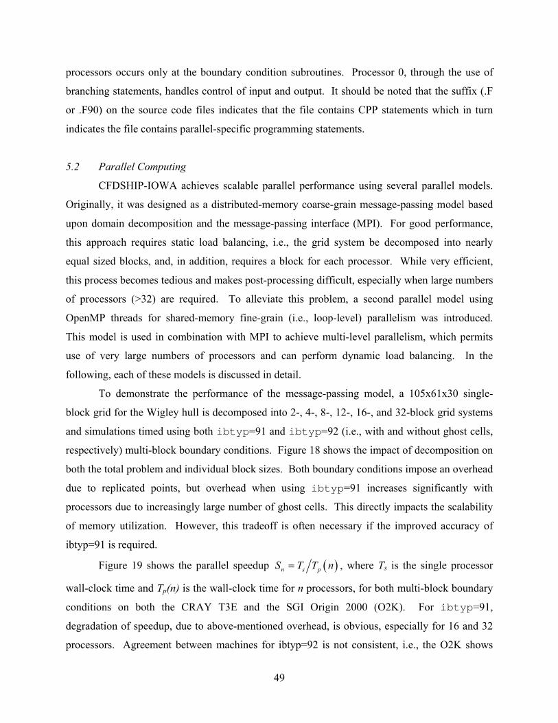
49

processors occurs only at the boundary condition subroutines. Processor 0, through the use of

branching statements, handles control of input and output. It should be noted that the suffix (.F

or .F90) on the source code files indicates that the file contains CPP statements which in turn

indicates the file contains parallel-specific programming statements.

5.2 Parallel Computing

CFDSHIP-IOWA achieves scalable parallel performance using several parallel models.

Originally, it was designed as a distributed-memory coarse-grain message-passing model based

upon domain decomposition and the message-passing interface (MPI). For good performance,

this approach requires static load balancing, i.e., the grid system be decomposed into nearly

equal sized blocks, and, in addition, requires a block for each processor. While very efficient,

this process becomes tedious and makes post-processing difficult, especially when large numbers

of processors (>32) are required. To alleviate this problem, a second parallel model using

OpenMP threads for shared-memory fine-grain (i.e., loop-level) parallelism was introduced.

This model is used in combination with MPI to achieve multi-level parallelism, which permits

use of very large numbers of processors and can perform dynamic load balancing. In the

following, each of these models is discussed in detail.

To demonstrate the performance of the message-passing model, a 105x61x30 single-

block grid for the Wigley hull is decomposed into 2-, 4-, 8-, 12-, 16-, and 32-block grid systems

and simulations timed using both ibtyp=91 and ibtyp=92 (i.e., with and without ghost cells,

respectively) multi-block boundary conditions. Figure 18 shows the impact of decomposition on

both the total problem and individual block sizes. Both boundary conditions impose an overhead

due to replicated points, but overhead when using ibtyp=91 increases significantly with

processors due to increasingly large number of ghost cells. This directly impacts the scalability

of memory utilization. However, this tradeoff is often necessary if the improved accuracy of

ibtyp=91 is required.

Figure 19 shows the parallel speedup ( )n s pS T T n= , where Ts is the single processor

wall-clock time and Tp(n) is the wall-clock time for n processors, for both multi-block boundary

conditions on both the CRAY T3E and the SGI Origin 2000 (O2K). For ibtyp=91,

degradation of speedup, due to above-mentioned overhead, is obvious, especially for 16 and 32

processors. Agreement between machines for ibtyp=92 is not consistent, i.e., the O2K shows

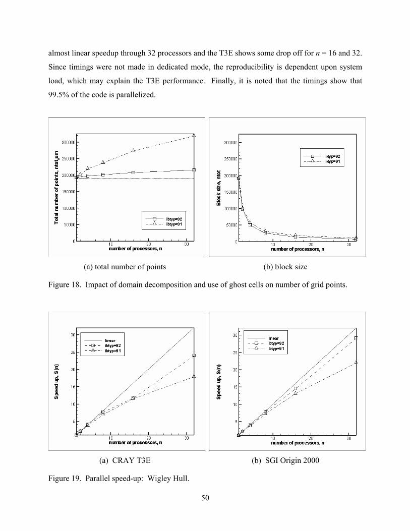
50

almost linear speedup through 32 processors and the T3E shows some drop off for n = 16 and 32.

Since timings were not made in dedicated mode, the reproducibility is dependent upon system

load, which may explain the T3E performance. Finally, it is noted that the timings show that

99.5% of the code is parallelized.

(a) total number of points (b) block size

Figure 18. Impact of domain decomposition and use of ghost cells on number of grid points.

(a) CRAY T3E (b) SGI Origin 2000

Figure 19. Parallel speed-up: Wigley Hull.

51

Shared-memory fine-grain (i.e., loop level) parallelism is introduced using OpenMP

which was designed to exploit certain characteristics of shared-memory architectures. Systems

that don't fit the classic shared-memory architecture (e.g., Beowulf clusters) may use OpenMP

but typical performance is very poor due to high latencies in communication. Currently,

CFDSHIP-IOWA implementation of OpenMP is only supported on the SGI Origin and IBM SP

machines through the use of the automatic parallelization option (-apo) in the Fortran 90

compiler. In particular, the SGI Origin uses a distributed-shared memory (DSM) architecture,

which can effectively utilize the shared-memory model.

To demonstrate performance, parallel simulations were performed on the NAVO O2K

using a surface-piercing flat plate (SPFP) with grid dimensions of 105x61x30 and with number

of processors ranging from 1 to 32. Figure 20 shows that speedup stalls at about 4 for this

problem on this machine. Analysis of cache utilization shows that the code is “non-cache

friendly” for scalable shared-memory applications. While this is an area of work for the future,

even a speed-up of 4 is useful for dynamic load balancing.

number of threads, n

Spee

dup,

S(n)

10 20 301

2

3

4

5

6

7

8

9

10

11

12

OMPLinear

Figure 20. Parallel speedup, shared memory on NAVO O2K.

Mixed-mode, or multi-level, parallelism utilizes both MPI and OpenMP to achieve

dynamic load balancing. Relative block size and the total number of processors specified by the

52

input variable total_num_procs sets the number of OpenMP threads that are used for each

block,

( )( )

_ max int _ _ ,1_

float ntotnum thrd total num procs

float ntot sum =

(88)

Table 8 shows an example for a 4-block grid system for an open-water propeller. The largest

block is 8.5 times bigger than the smallest block and comprises 65% of the total number of grid

points. The distribution of processors for total_num_procs = 16 and 32 are shown.

Unfortunately, performance studies have not yet been undertaken for a simple single-block grid

such as the SPFP or the Wigley Hull. However, based upon the OpenMP results, it should be

expected that using 10 or 20 processors on Block 4 may be inefficient and that domain

decomposition should be used to bring it’s sub-blocks closer to the size of blocks 1-3.

Table 8. Dynamic load balancing for 4-block grid system.

block block_size (ntot)

num_thrd

total_num_procs = 16

num_thrd

total_num_procs = 32

1 102951 2 4

2 102951 2 4

3 56203 1 2

4 480751 10 20

ntot_sum = 742856 Total procs used = 15 Total procs used = 30

5.3 Portability

The code was designed to be portable across the range of machines currently available at

the DOD High-Performance Computing Modernization Program (HPCMP) centers. Currently

this includes the SGI Origin 2000 & Origin 3000, Cray T3E, Cray SV1, Cray T90, and IBM SP2.

In addition, the code has been compiled on the DEC Alpha, HP Workstation, and Intel X86

personal computers, the latter of which uses Compaq Visual Fortran.

Portability is achieved through the use of MPI, the C preprocessor CPP, and the UNIX

make utility. Vendor-optimized MPI is available on nearly all platforms. Otherwise, the

generic MPICH libraries can be used. CPP is used to build either the parallel or serial versions

from a single source code. MPI- and serial-specific code is isolated through the use of

53

‘#IFDEF SERIAL’, ‘#IFDEF PARALLEL’, and ‘#ENDIF’ CPP directives. Although not

typically required, the source code for either version can be readily obtained by simply running

CPP with the appropriate directives (i.e., -DSERIAL or –DPARALLEL). In addition, directives

are used to set MPI data types to MPI_REAL for all machines except for the CRAY T3E, which

requires MPI_DOUBLE_PRECISION. The code is written in FORTRAN and compiles with

Fortran 90. The makefile will build platform specific versions by invoking the correct compiler

options and the CPP directives. The machines and options available are shown in Table 9.

Table 9. Supported platforms and make options.

Machine make argument (Serial/Parallel) SGI Origin 2000 O2K/O2K_MPI SGI Power Challenge Array PCA/PCA_MPI CRAY T3E T3E/T3E_MPI CRAY T90 T90/NA DEC Alpha DEC/DEC_MPI HP workstation HP/NA Intel X86 Processor None (Visual Fortran) Beowulf Cluster (Portland Group Compiler) CLUSTER/CLUSTER_MPI

5.4 Code distribution, extraction, compilation and execution

CFDSHIP-IOWA source code is distributed as a compressed tar file, which can be

uncompressed and extracted using the following UNIX command,

%tar –xvf | uncompress cfdship.tar.Z

The following files are included in the distribution

filename Description

readme Description of files

makefile UNIX makefile

cfdship_mods.F90 Definition of Fortran modules

cfdship_chimera.F90 Interface with PEGASUS

cfdship_bcs.f Boundary conditions

cfdship_frsf.f Free surface

cfdship_ke.F Discretization/solution of k-ε turbulence model

54

cfdship_ko.F Discretization/solution of k-ω turbulence model

cfdship_main.F Main program

cfdship_mom.f Discretization/solution of momentum equation

cfdship_mpsr.F Multi-processor versions of subroutines

cfdship_pres.f Discretization/solution of pressure equation

cfdship_ship.f Propeller body force, forces and moments

cfdship_stio.F Setup and input/output routines

cfdship_turb.F Turbulence closure

cfdship_util.f Solvers, interpolation routines,utilities

Tools/convert_chimera.F90 Converts XINTOUT file to either ASCII or unformatted format

Tools/decomp.f Partitions grid into sub-blocks for parallel computing

Tools/grd-atob.f90 Converts grid file from ASCII to unformatted format

Tools/grid-btoa.f90 Converts grid file from unformatted to ASCII format

Tools/grid-restrict.f Creates coarse and medium grids given fine grid

Tools/inlet-rst.f Creates restart file given inlet profile

Tools/prolong.f Interpolates coarse-grid solution onto medium and fine grids and creates restart files

Tools/redist.f90 Changes distribution of grid points

Tools/slicer.f90 Extracts subset of data from restart file

Tools/xyz-to-xrt.f Convert grid from Cartesian to cylindrical coordinates

The file extension indicates the presence of CPP statements (i.e., .F or .F90) and whether the

code is written in fixed (i.e., .f or .F) or free-formats (i.e., .f90 or .F90).

After uncompressing and extracting all files, the flow code is compiled using the

makefile along with machine specific option listed in Table 9. For example, to compile the flow

code on the SGI Origin 2000 with MPI parallelism, the following should be typed

%make O2K_MPI

Execution is platform dependent and requires site-specific preparation of job scripts and

queue submission. However, serial jobs are executed with the following command,

%cfd_ship >standard_output_file

whereas parallel jobs are executed using the mpirun command

55

%mpirun –np 12 cfd_ship >standard_output_file

In either mode, the code automatically looks for the NAMELIST input file cfd_ship.nml,

preparation and contents of which are described in the next section.

6. CREATING INPUT FILES AND POST-PROCESSING

The fourth and sixth steps of the CFD Process, as defined in Section 2, are focused on

creating input files and post-processing of simulation results, respectively. While these steps are

common to all CFD codes, the mechanics of undertaking these tasks are usually unique and can

potentially represent a significant amount of time in the overall CFD Process. Because of this,

an overall framework and graphical user interface, most notably in commercial codes, is often

utilized to simplify the process and hide low-level details from user. Another approach is to use

scripting languages to automate repetitive tasks like grid generation and setting of parameters. In

recognition of the challenge this presents to small groups developing research codes, there are

current efforts sponsored by HPCMP CHSSI to develop extensible frameworks for managing

input file creation, file formats, and communication between tools. Unfortunately, until such

software is available to the CFD community, users of CFDSHIP-IOWA will be required to have

first hand knowledge of how to create and manipulate data files.

6.1 Input files

CFDSHIP-IOWA reads 5 different input files to provide data for computational grid,

initial conditions, boundary conditions, flow conditions, selection of models, and specification of

numerical parameters and post-processing variables. Table 10 summarizes the filenames,

Fortran unit numbers, and descriptions of the input files. Detailed presentation of the file format

is provided in Appendix A. Here, the purpose of, and the method for creating, each file is

described.

56

Table 10. Input files

Filename Unit Number Description cfd_ship.nml (fixed filename) 8 Namelist input for runtime variables grid file (no filename restrictions) 15 Grid file in ASCII Plot3D format FNAMEO.bcs 25 Boundary condition data FNAMEO.xintout 45 Chimera interpolation coefficients FNAMEI.rsto 35 Restart file from previous simulation

The master control file for CFDSHIP-IOWA is named cfd_ship.nml. Its purpose is

to specify initial conditions, flow conditions, selection of models, and specification of numerical

parameters and post-processing variables. All input parameters belong to one of nine namelists

(control, flow_parameters, grid parameters, iteration, solver,

turbulence, free_surface, propeller, filenames). A namelist is a list of

variable names that are always read or written as a group. Namelist input provides a convenient

interface for a research CFD code since default values can be set for most variables, and new

variables can be added in future versions without making previous input files obsolete. In

general, cfd_ship.nml is created by copying an existing file and modifying variables using a

text editor as required. Detailed description of the namelists, variables, and default values are

included in Appendix A.2 and an example can be found in Appendix B.1.

The grid file contains (x, y, z) or (x, r, θ) coordinates of the structured-grid multi-block

system. Note that for Cartesian and cylindrical-polar grids, the icoord variable in namelist

CONTROL must be set to (1/2) or (3/4), respectively. The grid file format is ASCII Plot3D, the

details of which are specified in Appendix A.1. Method for generating grid file is at the

discretion of the user.

The boundary condition file specifies boundary condition types on all faces, which may

be arbitrarily broken into rectangular sub-patches, of the computational domain, including multi-

block interfaces. For each patch, the following information must be specified in the

FNAMEI.bcs input file: ibtyp is the boundary condition type, ibdir is the inward pointing

normal direction in computation coordinate direction (+1/-1, +2/-2, or +3/-3), ibcs, ibce,

jbcs, jbce, kbcs, kbce are the starting and ending indices in the (ξ,η,ζ) coordinates

directions, ibcord is a flag used to set the discretization order-of-accuracy for Neumann

boundary conditions, i.e., ibcord=0 for first order and 1 for second order, and ifsfilter is

57

a flag which is only used for free-surface boundaries and sets the filter type as described in

Section 4.4. For multi-block and periodic conditions, the following additional information is

required: ndmesh is the donor block number, idbdir is the inward-pointing normal in the

donor block, and idcs, idce, jdcs, jdce, kdcs, kdce are the starting and ending

indices for the donor block. Detailed description of the file format is provided in Appendix A.3

and an example is provided in Appendix B.3. The recommended procedure for setting boundary

conditions and creating FNAMEI.bcs is to use GRIDGEN software from Pointwise, Inc.

wherein CFDSHIP-IOWA is one of the supported analysis software options (AS/W). This

allows use of the GRIDGEN graphical user interface which greatly reduces time and errors.

The final two input files are optional. Restart files are only required if initial conditions,

or prescribed boundary conditions (ibtyp=14), are set by previous simulations. If a restart file

is to be read, the variable mode in NAMELIST CONTROL must be set to 1. Restart file is

typically created by previous simulation, however, users can write custom software similar to the

provided tool inlet-rst.f which can write a restart file for specifying an inlet profile. The

file containing Chimera overset grid interpolation coefficients is required only when using

overset grids. This file is created following flowchart depicted in Figure 13.

6.2 Output files & post-processing

Output files provide access to the simulation results and can be used to assess iterative

convergence, determine forces and moments, and analyze details of the flow field. As shown in

Table 11, there are 8 output files that contain simulation results, however, the restart file is

typically not used for post-processing. Four of the files are used for assessing iterative

convergence. FNAMEO.res contains residuals, average divergence, and evaluation of mass and

momentum balance over the computational domain, using the Reynolds-transport theorem, at

each time step (or global iteration). FNAMEO.forces and FNAMEO.moments provide forces

and moments acting on the no-slip surfaces at each time step and are useful for assessing

iterative convergence of integral variables. Forces and moments are broken down into 9

components with contributions due to skin friction, piezometric pressure, and hydrostatic

pressure in each of the 3 coordinate directions. FNAMEO.conv and FNAMEO.fsconv

contain iterative convergence history of the point variables (U, P, Uτ) and free-surface wave

58

elevation ζ, respectively. Writing frequency is specified by the namelist variable

it_save_conv, which is otherwise set to a default value of 500 time steps (or global

iterations).

The remaining output file is the global solution file, which contains all independent and

dependent flow variables. By default, the solution is written only on the last time step for steady

flows or every 500 time steps for unsteady flows. If solutions are required more frequently, for

example to construct animations, the namelist variable it_save_tec can be used to specify

desired time-step frequency. This file is formatted as an ASCII Tecplot file and therefore is

directly readable by the commercial visualization software Tecplot.

Table 11. Output files

Filename Unit Number Description FNAMEO.rsto 16 Restart file FNAMEO.tec 26 Global solution file in TECPLOT format FNAMEO.res 36 Solution residuals FNAMEO.conv 46 Iterative history of pressure, friction velocity, and

velocity along no-slip surfaces FNAMEO.forces 56 Iterative history of forces FNAMEO.moments 57 Iterative history of moments FNAMEO.fsconv 66 Iterative history of free surface FNAMEO_bodyforces.tec 86 Grid, blanking variable indicating whether point is

in/out of propeller disk, and body-force components.

7. RECOMMENDED VERIFICATION AND VALIDATION PROCEDURES

CFD is fast becoming an integral tool in the engineering design process as it is applied to

increasing complex geometry and physics. As with use of experimental fluid dynamics (EFD) in

making design decisions, assessment of quality of results is imperative, which has accelerated

progress on development of verification and validation (V&V) methodology and procedures for

estimating numerical and modeling errors and uncertainties in CFD simulations. However, in

spite of the progress, the various viewpoints have not yet fully converged and current

methodology and procedures are not yet standardized.

Here, however, the recommended V&V procedures are those provided by Stern et al.

(2001) and for which Wilson et al. (2001) presented a detailed case study for a RANS simulation

of an established benchmark for ship hydrodynamics. The methodology and procedures

59

presented therein provides a pragmatic approach for estimating simulation errors and

uncertainties. The philosophy is strongly influenced by EFD uncertainty analysis. The approach

allows for treatment of simulation errors as either stochastic or deterministic and properly takes

into account uncertainties in both the simulation and the data in assessing the level of validation.

A brief summary of the methodology and procedures is provided in the following.

7.1 Methodology

The simulation error Sδ is defined as the difference between a simulation result S and the

truth T and is composed of modeling SMδ and numerical SNδ errors ( S SM SNS Tδ δ δ= − = + )

with corresponding simulation uncertainty given by 2 2 2S SM SNU U U= + . For certain conditions,

both the sign and magnitude of the numerical error can be estimated as SNSNSN εδδ += * where

*SNδ is an estimate of the sign and magnitude of SNδ and εSN is the error in that estimate. The

simulation value is corrected to provide a numerical benchmark SC, which is defined by

*C SNS S δ= − (89)

with error equation SNSMCS TSC

εδδ +=−= and corresponding uncertainty equation

222NSSMS CC

UUU += where CSU is the uncertainty in the corrected simulation and NSC

U is the

uncertainty estimate for εSN.

Verification is defined as a process for assessing simulation numerical uncertainty SNU and,

when conditions permit, estimating the sign and magnitude ∗SNδ of the simulation numerical

error itself and the uncertainty in that error estimate NSCU . Numerical error is decomposed into

contributions from iteration number Iδ , grid size Gδ , time step Tδ , and other parameters Pδ ,

which gives the following expression for the simulation numerical uncertainty

2 2 2 2 2SN I G T PU U U U U= + + + (90)

For situations when the solution is corrected to produce a numerical benchmark CS , the

estimated simulation numerical error *SNδ and corrected uncertainty NSC

U are given by

* * * * *SN I G T Pδ δ δ δ δ= + + + (91)

2 2 2 2 2C C C C CS N I G T PU U U U U= + + + (92)

60

Validation is defined as a process for assessing simulation modeling uncertainty SMU by

using benchmark experimental data and, when conditions permit, estimating the sign and

magnitude of the modeling error SMδ itself. The comparison error E is given by the difference in

the data D and simulation S values

( )D SMA SPD SNE D S δ δ δ δ= − = − + + (93)

where SMδ has been decomposed into the sum of δSPD, error from the use of previous data such

as fluid properties, and δSMA, error from modeling assumptions. To determine if validation has

been achieved, E is compared to the validation uncertainty UV given by

2 2 2 2V D SN SPDU U U U= ++ (94)

If |E| < VU , the combination of all the errors in D and S is smaller than UV and validation is

achieved at the VU level. If UV <<|E|, the sign and magnitude of E=δSMA can be used to make

modeling improvements. For the corrected approach, the equations equivalent to equations (93)

and (94) are

( )C C D SMA SPD SNE D S δ δ δ ε= − = − + + (95)

2 2 2 2 2 2C C CV E SMA D SPD S NU U U U U U= − = + + (96)

7.2 Procedures

The overall CFD V&V procedures can be conveniently grouped into four consecutive

steps: preparation, verification, validation, and documentation.

Verification is accomplished through parameter convergence studies using multiple solutions

(at least 3) with systematic parameter refinement by varying the kth input parameter kx∆ while

holding all other parameters constant. Iterative errors must be accurately estimated or negligible

in comparison to errors due to input parameters before accurate convergence studies can be

conducted. Changes between medium-fine 12

ˆˆ21 kk SS

k−=ε and coarse-medium

23ˆˆ

32 kk SSk

−=ε

solutions are used to define the convergence ratio

21 32k kkR ε ε= (97)

61

and to determine convergence condition where 1

ˆkS ,

2ˆ

kS , 3

ˆkS correspond to solutions with fine,

medium, and coarse input parameter, respectively, corrected for iterative errors. Three

convergence conditions are possible:

(i) Monotonic convergence: 0 < kR < 1

(ii) Oscillatory convergence: kR < 0 (98)

(iii) Divergence: kR > 1

For condition (i), generalized RE is used to estimate kU or ∗kδ and

CkU . For condition (ii),

uncertainties are estimated simply by attempting to bound the error based on oscillation

maximums SU and minimums SL, i.e., ( )12k U LU S S= − . For condition (iii), errors and

uncertainties cannot be estimated.

For convergence condition (i), generalized RE is used to estimate the error 1kREδ ∗ due to

selection of the kth input parameter and order-of-accuracy pk

1

21

1k

k kRE pkrε

δ ∗ =−

(99)

)rln(

)ln(p

k

2132k

kkεε

= (100)

Correction of equation (99) through a multiplication factor Ck accounts for effects of higher-

order terms and provides a quantitative metric to determine proximity of the solutions to the

asymptotic range

−== ∗∗

121

11 k

k

k pk

kREkk rCC

εδδ (101)

where the correction factor is given by

1

1−

−=

estk

k

pk

pk

k rr

C (102)

and estkp is an estimate for the limiting order of accuracy as spacing size goes to zero and the

asymptotic range is reached so that 1kC → . When solutions are far from the asymptotic range,

62

kC is sufficiently less than or greater than 1, only the magnitude of the error is estimated through

the uncertainty kU

1 1

(1 )k kk k RE k REU C Cδ δ∗ ∗= + − (103)

When solutions are close to the asymptotic range, kC is close to 1 so that ∗kδ is estimated using

equation (101) and CkU is estimated by

∗−=1

)1(kC REkk CU δ (104)

Alternatively, a factor of safety approach proposed in Roach (1998) can be used to define kU

and CkU .

Validation is accomplished through comparisons with benchmark EFD data, including

experimental uncertainty estimates UD. If the three variables UV, |E|, and Ureqd (programmatic

validation requirement) are considered, there are six combinations. For three cases, |E|<UV and

validation is achieved at the UV level, but for only one of these UV <Ureqd so that validation is

also achieved at Ureqd. In these cases, attempting to estimate modeling errors δSMA is not feasible

from an uncertainty standpoint. For the three other cases, UV <|E| and using the sign and

magnitude of E to estimate δSMA is feasible from an uncertainty standpoint. In one of these cases,

UV<|E|<Ureqd so that validation is successful at the |E| level from a programmatic standpoint.

Similar conclusions can be reached using the corrected comparison error and corrected validation

uncertainty.

8. EXAMPLE SIMULATION: OPEN-WATER PROPELLER P5168

In this section, an example simulation for DTMB open-water propeller P5168 is

presented and discussed. The intention is to demonstrate some of the capabilities of the code

including overset gridding, non-inertial relative frames, and detailed high-fidelity resolution of

both geometry and physics. Discussion follows the CFD process defined in Figure 1. Input files

for both the example and other training problems, including some with free-surface effects, may

be downloaded from the CFDSHIP-IOWA website, http://www.iihr.uiowa.edu/~cfdship.

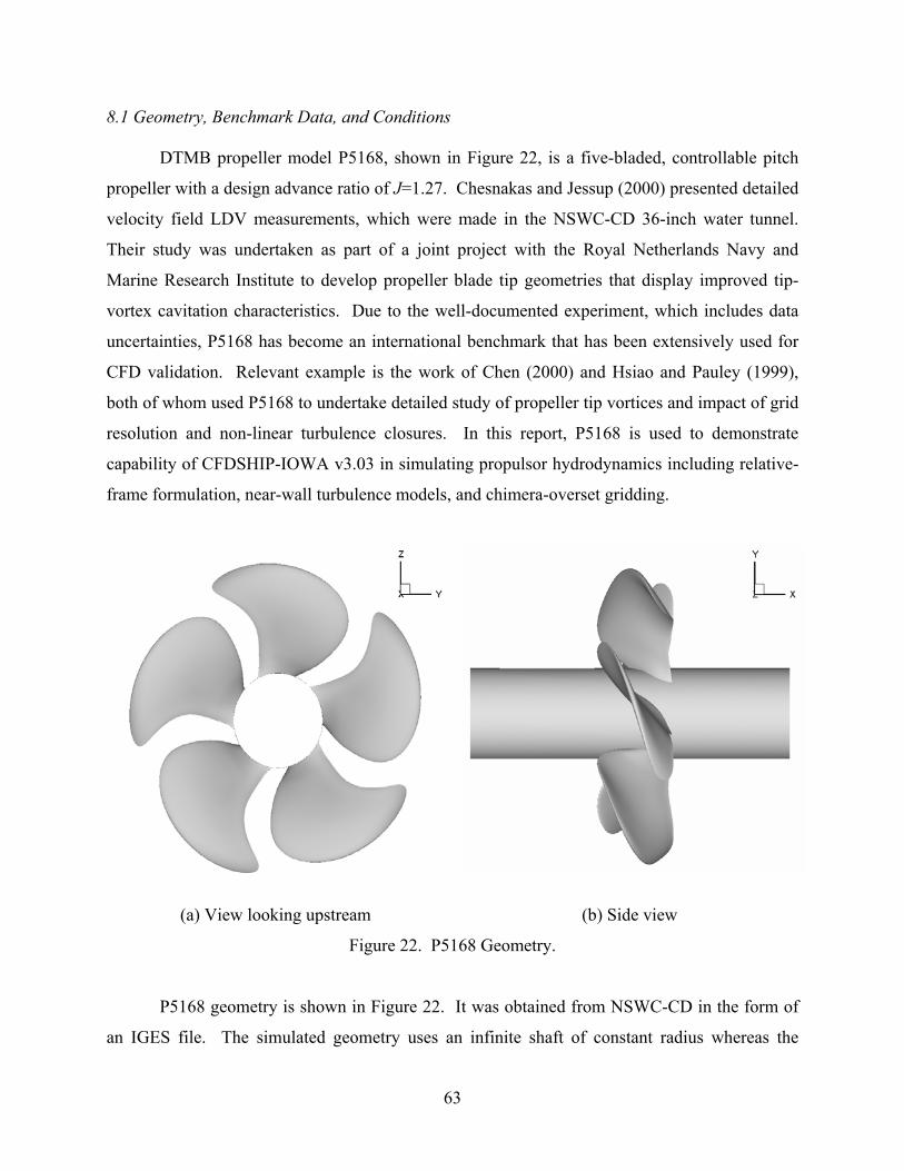
63

8.1 Geometry, Benchmark Data, and Conditions

DTMB propeller model P5168, shown in Figure 22, is a five-bladed, controllable pitch

propeller with a design advance ratio of J=1.27. Chesnakas and Jessup (2000) presented detailed

velocity field LDV measurements, which were made in the NSWC-CD 36-inch water tunnel.

Their study was undertaken as part of a joint project with the Royal Netherlands Navy and

Marine Research Institute to develop propeller blade tip geometries that display improved tip-

vortex cavitation characteristics. Due to the well-documented experiment, which includes data

uncertainties, P5168 has become an international benchmark that has been extensively used for

CFD validation. Relevant example is the work of Chen (2000) and Hsiao and Pauley (1999),

both of whom used P5168 to undertake detailed study of propeller tip vortices and impact of grid

resolution and non-linear turbulence closures. In this report, P5168 is used to demonstrate

capability of CFDSHIP-IOWA v3.03 in simulating propulsor hydrodynamics including relative-

frame formulation, near-wall turbulence models, and chimera-overset gridding.

(a) View looking upstream (b) Side view

Figure 22. P5168 Geometry.

P5168 geometry is shown in Figure 22. It was obtained from NSWC-CD in the form of

an IGES file. The simulated geometry uses an infinite shaft of constant radius whereas the

64

experimental geometry included a cylindrical fairwater that extended 96.8mm downstream of the

hub. In addition, the tested geometry, as shown in Figure 1 of Chesnakas and Jessup (2000), had

a small increase in hub radius near the propeller, a feature which is not included in the CFD

model. Since the focus here is simulation at near-design operating conditions, it is assumed that

the inflow is uniform in the circumferential direction and that the flow is steady. This allows the

computational domain to be reduced to a single blade passage through the use of rotationally

periodic boundary conditions. The overall domain, which was shown in Figure 2, extends 0.65D

upstream, 1.5D downstream, and 1.5D outward in the radial direction.

The flow conditions and fluid properties are based upon the experimental conditions at

J=1.1, which is slightly off the design point and is used since it results in a stronger tip vortex

than J=1.27. This condition also corresponds to n=1450 rpm, U=10.70m/s, T=4715N, Q=481N-

m. Non-dimensional parameters used in CFDSHIP-IOWA are Re=3.0x106 and ωx=-2π/J=-

5.712. Flow conditions are specified in the namelist input file, cfd_ship.nml. The file

used for P5168 is included in the Appendix B.1 as an example.

For detailed propulsor simulations (as opposed to using a propeller body force), the only

model choice is that of turbulence model. For the simulations here, the standard blended k-ω/k-ε

turbulence model was used, i.e., itm=2, itm_switch=0.

Steady flow simulations use free-stream initial conditions where all flow variables are set

to UINF=1 and VINF=WINF=0. This is achieved by setting mode=0 in the cfd_ship.nml

file. As shown in Figure 2, the following boundary conditions were used for a single-blade

propeller simulation: relative-frame no-slip (ibtyp=22) on the blade and hub surfaces, prescribed

velocity (ibtyp=14) on the upstream inlet plane, exit (ibtyp=12) on the downstream exit plane,

far-field (ibtyp=13) on the outer boundaries, and rotationally-periodic (ibtyp=52) on the periodic

faces. The prescribed velocity profile is

( )2

1 1 h

h

r rU rr rδ

−= − − −

(105)

where rh = 0.122199 is the hub radius and rδ = 0.185 is the boundary layer thickness at the inlet

plane. Inlet profile in equation (105) was determined by Chen (2000) to give proper loading at

the blade root. Remaining block boundaries are either patched multi-block (ibtyp=92) or

Chimera outer boundaries, the latter of which requires use of PEGASUS v5.1 from NASA Ames

65

and which will be further discussed in the next paragraph. An example boundary condition file

is included in the Appendix B.3.

8.2 Computational Grids and Input Parameters

Generating high-quality patched-multi-block grids for open-water propellers is

challenging due radial pitch distribution, especially beyond the tip, requirements for rotational

periodicity, and need for boundary-layer resolution near blade and hub surfaces. Together, these

issues make it difficult to control both skewness and expansion ratios. CFDSHIP-IOWA v3.03

is fairly sensitive to grid quality such that grids used in earlier versions (especially those based

upon the Finite Analytic method) often result in unstable simulations.

(a) Passage blocks (b) Blade blocks

Figure 23. P5168 Overset Grid System.

Although a best practices document for CFDSHIP-IOWA does not yet exist (e.g., a

document similar to Chan et al., 2002), the following guidelines can be provided. As a rule of

thumb, CFDSHIP-IOWA gives most accurate results using expansion ratios less than 1.5 and, in

general, values greater than 3 should be avoided since simulation stability is sensitive to this

parameter. At multi-block interfaces, spacing on each side of the interface should be similar.

For boundary-layer resolution, near-wall spacing should be set such that the non-dimensional

66

wall coordinate y u yτ ν+ = is less than 2.5 and ideally near 1.0. Overset gridding provides an

approach to achieve these metrics and obtain high-quality grids, especially for complex

geometries.

The overset grid system used for P5168 is shown in Figure 23. This system is based

upon a series of H-type “passage” blocks, which are generated without regard for the blade

geometry, and O-type “blade” blocks, which are generated without regard for the periodic

surfaces.

Table 11. P5168 Grid Parameters

fine medium coarse

Block # Name imax jmax kmax total imax jmax kmax total imax jmax kmax total

1 passage1 61 81 81 400,221 43 58 58 144,652 31 41 41 52,111

2 passage2 61 81 81 400,221 43 58 58 144,652 31 41 41 52,111

3 passage3 61 81 81 400,221 43 58 58 144,652 31 41 41 52,111

4 passage4 61 81 81 400,221 43 58 58 144,652 31 41 41 52,111

5 inner_p 41 61 31 77,531 29 43 22 27,434 21 31 16 10,416

6 inner_s 41 61 31 77,531 29 43 22 27,434 21 31 16 10,416

7 tip_p1 45 61 31 85,095 32 43 22 30,272 23 31 16 11,408

8 tip_s1 45 61 31 85,095 32 43 22 30,272 23 31 16 11,408

9 tip_p2 45 61 31 85,095 32 43 22 30,272 23 31 16 11,408

10 tip_s2 45 61 31 85,095 32 43 22 30,272 23 31 16 11,408

11 tip_p3 41 61 45 112,545 29 43 32 39,904 21 31 23 14,973

12 tip_s3 41 61 45 112,545 29 43 32 39,904 21 31 23 14,973

13 root_p1 45 61 65 178,425 32 43 46 63,296 23 31 33 23,529

14 root_p2 41 61 65 162,565 29 43 46 57,362 21 31 33 21,483

15 root_p3 45 61 65 178,425 32 43 46 63,296 23 31 33 23,529

16 root_s1 45 61 65 178,425 32 43 46 63,296 23 31 33 23,529

17 root_s2 41 61 65 162,565 29 43 46 57,362 21 31 33 21,483

18 root_s3 45 61 65 178,425 32 43 46 63,296 23 31 33 23,529

19 phantom 121 51 11 67,881 121 51 11 67,881 121 51 11 67,881

Total 3,360,246 Total 1,202,280 Total 441,936

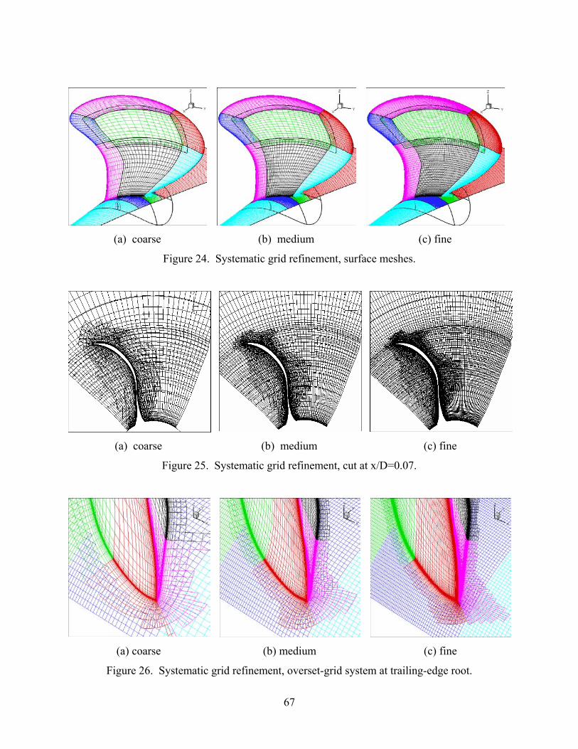
67

(a) coarse (b) medium (c) fine

Figure 24. Systematic grid refinement, surface meshes.

(a) coarse (b) medium (c) fine

Figure 25. Systematic grid refinement, cut at x/D=0.07.

(a) coarse (b) medium (c) fine

Figure 26. Systematic grid refinement, overset-grid system at trailing-edge root.

68

This approach improves grid quality, as measured by orthogonality and expansion ratios,

accelerates grid-generation process, and permits the use of overset refinement meshes (e.g., Kim

et al., 2003). The grid system is generated using GRIDGEN from Pointwise, Inc. and was

designed for a 3-grid verification study as shown in Table 11 and with near-wall spacing less

than 5x10-6 on all grids. The fine grid was generated using GRIDGEN. The medium and coarse

grids were obtained from the fine grid using a 2 refinement ratio in each coordinate direction.

A grid-sequencing tool based upon linear interpolation in computational space is used. This

results in a coarse grid, which is systematically similar to the fine grid due to the fact it is created

through grid halving. In contrast, the medium grid is not exactly systematically similar to the

fine grid due to handwork in GRIDGEN required to correct geometry errors introduced in using

linear interpolation. Figure 24 shows the surface grids for each grid system. Total number of

grid points range from 3.36 to 0.44 million points for the fine and coarse grids, respectively.

Before running CFDSHIP-IOWA, overset-grid interpolation coefficients must be

computed using overset-grid communication software. Execution of PEGASUS version 5.1 is

accomplished following the instructions in Section 4.7 of this report and using the sample input

file found in Appendix B.2. Therein, it can be seen that a novel approach has been taken where

two separate hole cutters ($HCUT NAME) have been defined. The first one is a traditional

external-type HCUT named “blade_cutter.” This HCUT creates a hole in the passage blocks due

to the blade surfaces and uses a phantom mesh at the root of the blade so as to create the required

“leak-free” surface. The second one is an internal-type hole cutter named “passage_cutter”

whose purpose is to trim away points in the blade blocks that extend past the periodic surfaces.

Figures 25 and 26 show the composite grid system for coarse, medium, and fine grids. Note that

the fringe boundaries are a function of grid resolution. This is due to Level-2 interpolation.

Impact on verification grid studies is unknown.

Numerical parameters are specified in the cfd_ship.nml file of which an example for

P5168 can be found in the Appendix B.1. Therein, it can be seen that the following numerical

parameters were specified: 2nd-order upwind spatial accuracy (ispat_order=3); 1st-order

backward temporal accuracy, or steady flow (itemp_order=1); Cartesian relative-frame

coordinate system (icoord=2); time step of delt=0.01, free stream velocities components of

uinf=1 and vinf=winf=0; starting and ending iterations of its=1 and itend=10000;

69

iterative frequency of writing convergence history (it_save_conv), restart file

(it_save_rst), and tecplot file (it_save_tec) of 50, 500, and 5000, respectively; number

of momentum (ituvw), velocity-pressure coupling (itvpc), pressure (itpr), and turbulence

(itturb) sub-iterations of 5, 3, 5, and 5, respectively; relaxation factors of rfv=0.2,

rfvb=0.2, rfp=0.1, and rfpb=0.05; fully half-cell formulation of the pressure equation

(gama_pr=1.0); line-solvers are turned on for each coordinate direction iswp1=1, iswp2=1,

iswp3=1; pressure reference coordinate location is specified to be mref=1, iref=1,

jref=41, kref=21; and convective discretization of the k and ω equations is set to 1st-order

upwind (ispat_order_tm=1).

8.3 Computing Platforms

Simulations were undertaken using two computer systems, the 512-processor SGI Origin

3800 at the Army Research Laboratory Major-Shared Resource Center (ARL-MSRC,

http://www.arl.hpc.mil/) and the 72-processor Linux Beowulf cluster at the Penn State Applied

Research Laboratory. The former is a distributed-shared parallel computer, which is capable of

using mixed-mode parallelism (i.e., code is compiled as make O2K_MPI_OMP) and the latter is

a distributed parallel computer, which is capable of MPI parallelism only (i.e., code is compiled

as make CLUSTER_MPI). As shown in Table 11, block-size distribution is not uniform, i.e.,

passage blocks are a factor of 5 larger than the smallest block. Therefore, on the SGI, some

degree of load balancing was achieved through the use of OMP threads, which is an automatic

process if total_num_proc is specified in the cfd_ship.nml file. Setting

total_num_proc = 38, 4 OpenMP threads were used on the passage blocks, 1 thread on

blocks 5-10, and 2 threads on the remaining blocks. The computational rate was 5.5x10-5

processor-secs/grid-point/iteration. For comparison, on the Linux cluster, where OMP threads

cannot be used for load balancing, computational rate was 6.9x10-4 processor-secs/grid-

point/iteration.

8.4 Verification and Validation Results

Typically, iterative convergence is assessed using both force and moment histories and

residuals based upon the change in variable between iterations. However, in simulations with

70

overlapping surface grids, iterative history of forces and moments are not currently available due

to the lack of a run-time interface with FOMOCO. As discussed in Section 4.8, FOMOCO,

which is a part of the suite of Chimera Grid Tools, computes forces and moments on overlapping

grids only as a post-processing step. Therefore, iterative convergence is demonstrated through

the use of residuals. Coarse grid simulation was run for 15,000 iterations and shows 4 orders

magnitude drop for all variables. A grid sequencing approach was used wherein coarse- and

medium-grid solutions were used as medium- and fine-grid simulation initial conditions,

respectively. Medium simulation was run 5000 iterations and fine simulation was run 1000

iterations. Based upon previous experience, it is assumed that UI is approximately zero for all

grids.

Table 12. P5168 Thrust and Torque Coefficients and Comparison to Data.

EFD Data Coarse Medium Fine

KT

E%=(D-S)/D*100

ε

0.313 0.310

1.0%

0.318

-1.6%

0.008

0.322

-2.9%

0.004

10KQ

E%=(D-S)/D*100

ε

0.783 0.765

2.3%

0.793

-1.3%

0.028

0.805

-2.8%

0.012

Comparing thrust and torque coefficients to EFD data and calculating changes between

grids ε, as done in Table 12, it is shown that near-blade integral quantities display monotonic

grid convergence as indicated by the convergence ratios of RG = 0.5 and RG = 0.42 for thrust and

torque, respectively. Based upon the rules of Equation (99), grid uncertainty can be estimated

using RE and is shown in Table 13. Since UD is not available for KT and KQ, validation

uncertainty UV is not calculated.

Table 13. Verification of P5168 Thrust and Torque Coefficients.

pG δ∗RE CG UGC UI USN

KT 2.0 0.004 1.0 0.0 0.0 0.004

KQ 2.4 0.015 1.29 0.0043 0.0 0.015

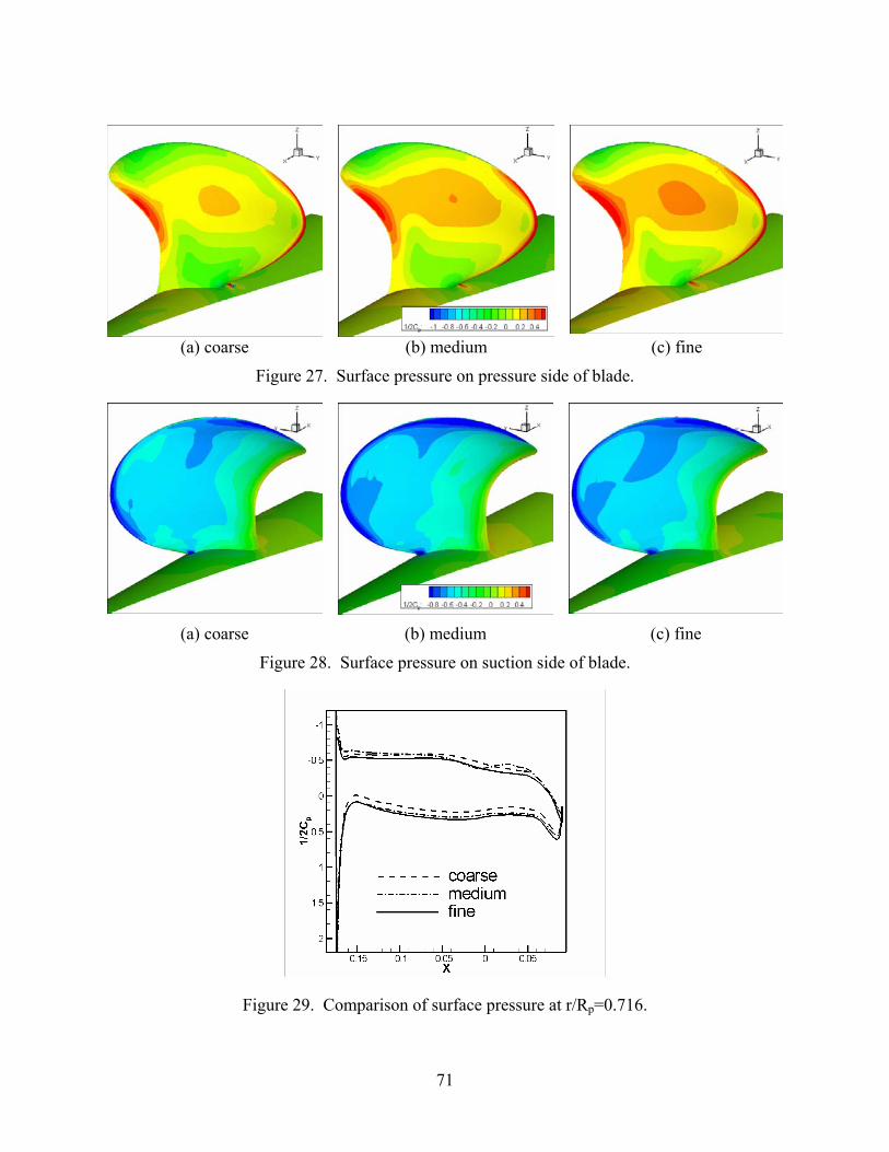
71

(a) coarse (b) medium (c) fine

Figure 27. Surface pressure on pressure side of blade.

(a) coarse (b) medium (c) fine

Figure 28. Surface pressure on suction side of blade.

Figure 29. Comparison of surface pressure at r/Rp=0.716.

72

Surface pressure contours are shown, for each grid system, in Figures 27 and 28. In

general, typical blade pressure distributions are shown with maximum loading at approximately

¾ span, high magnitude on the pressure-side leading- and trailing-edges, and low magnitude on

the suction-side tip. Contours also display monotonic grid convergence with fine grid displaying

highest resolution of detail. Figure 29 shows a comparison of surface pressure at r/Rp=0.716.

Pressure-side of blade displays monotonic grid convergence whereas suction side displays more

oscillatory behavior along the chord.

Figure 30 highlights the grid convergence of the tip and root vortices using iso-surfaces

of intrinsic swirl parameter (Berdahl and Thompson, 1993) at level τ = 8.0 colored by

normalized helicity H Uω= × , the latter of which indicates direction of rotation. Counter-

rotating root vortices display increasing strength, as indicated by increased persistence and

organization in the downstream direction, with increasing grid resolution. Similar observation

can be made for tip vortex, i.e., fine grid shows tip vortex with longest persistence, however, the

very short persistence of the coarse grid suggests grid in tip-vortex region is not in the

asymptotic range.

(a) coarse (b) medium (c) fine

Figure 30. Tip- and root-vortex visualization using iso-surface of intrinsic swirl parameter (τ = 8.0) colored by normalized helicity.

Figure 31 shows a comparison of simulation to data for axial-velocity contours at

x/D=0.1193. In general, all three solutions show resolution of the global trends, i.e., thin blade

wakes with increasing wake thickness near hub, maximum velocity on the suction side, and

73

(a) coarse grid (b) medium grid

(c) fine grid (d) EFD data Figure 31. Axial velocity contours at x/D=0.1193.

contours typical of a tip vortex at r/D=0.5. Moreover, resolution of blade wakes and tip-vortex

show grid convergence in that a general trend of improved resolution with grid can be observed.

However, detailed comparison of certain contour levels between the 3 solutions indicates some

degree of oscillatory grid convergence. This is more clearly shown in Figure 32 which shows

the axial velocity as a function of circumferential position at a constant radius of r/D = 0.465.

This figure shows the blade-to-blade variability of the data. Overall, the 3 solutions display a

non-monotonic divergent condition, which may be due to both a coarse grid solution outside of

74

the asymptotic range and grids which are not exactly systematically similar; observations

supported by Figure 30 and previously discussed in section 8.2, respectively. However, medium

and fine grids appear to be converging towards the data which suggests that a finer grid 4th

solution at approximately 9.5 million grid points, which would be a very large grid for a single-

blade simulation, would provide 3 solutions in the asymptotic range. This represents the

principal challenge of RE based error estimation and points to the need for continued research

and development in automatic generation of geometrically similar overset grids and interpolation

coefficients, and single-grid error estimation techniques (e.g., Celik et al., 2003).

Figure 32. Comparison of circumferential distribution of axial velocity at r/D=0.465 and

x/D=0.1193.

75

9. CONCLUDING REMARKS

CFDSHIP-IOWA is a general-purpose unsteady Reynolds-averaged Navier-Stokes CFD

code that has been developed to handle a broad range of ship hydrodynamics problems. Purpose

of this report was to provide: detailed documentation of the modeling, numerical methods, and

code development; user instructions on creating input files and post-processing; recommended

verification and validation procedures; and an example simulation. As a framework for

achieving successful simulations, an approach based upon formulation of an initial boundary

value problem and execution of a well-defined CFD process was developed and followed

throughout the report. An example simulation, and other recent applications, demonstrates the

capability of CFDSHIP-IOWA v3.03 to simulate practical ship hydrodynamics problems.

Successful use in both thesis and project research and transition to other organizations

demonstrates the success of the overall design objectives.

Largely due to successes such as those shown and referred to herein, role of CFD in

analysis and design of future marine vehicles continues to expand. Beyond higher-fidelity

simulation of resistance and propulsion problems, albeit including new applications and off-

design conditions, it is anticipated that future simulations will move towards including

environmental effects (e.g., seaway, stratification, shallow water), simulation-based design and

optimization, resolving complex maneuvering scenarios of multiple-body configurations (e.g.,

submarine or surface-ship launch of adjunct vehicles), and supporting improved modeling of

acoustic and non-acoustic signatures. However, in spite of continued advancements in HPC

hardware, the magnitude of these problems are expected to be on the order of 20-50 million grid

points and therefore require continued development of more accurate numerics and faster

computing algorithms. Areas of future development include improved algebraic solvers,

adaptive gridding, ideally using a single-grid error-estimation equation, implementation of

geometry manipulation protocols for specification of vehicle configurations and

maneuvering/seakeeping scenarios, multi-phase level-set methods for robust free-surface

simulations, and hybrid RANS-LES models for numerous applications.

76

REFERENCES

Alessandrini B, Delhommeau G, Viscous Free Surface Flow past a Ship in Drift and in Rotating Motion, Proc. 22nd Sympo. on Naval Hydro., Washington, DC, 1998. Beddhu, M., Jiang, M.Y., Taylor LK, and Whitfield DL, Computation of Steady and Unsteady Flows with a Free Surface Around the Wigley Hull, Applied Mathematics and Computation, Vol. 89, 1998, pp. 67-84. Berdahl, C.H., and Thompson, D.S., “Eduction of Swirling Structure Using the Velocity Gradient Tensor,” AIAA Journal, Vol. 31, No. 1, 1993. Bush, R.H., Power, G.D., and Towne, C.E., “WIND: The Production Flow Solver of the NPARC Alliance,” AIAA-98-0835, 36th Aerospace Sciences Meeting & Exhibit, Reno, NV, January 1998. Celik, I., Hu, G., and Badeau, A., “Further Refinement and Benchmarking of a Single-Grid Error Estimation Technique,” AIAA Paper 2003-0628, Reno, NV, 2003. Chan, W.M., Gomez, R.J., Rogers, S.E., and Buning, P.G., “Best Practices in Overset Grid Generation,” AIAA Paper 2002-3191, Proceedings 32nd AIAA Fluid Dynamics Conference, St. Louis, MO, 2002. Chan, W. M. and Buning, P. G., User's Manual for FOMOCO Utilities - Force and Moment Computation Tools for Overset Grids, NASA TM 110408, July, 1996 Chen, B., “RANS Simulations of Tip Vortex Flows for a Finite-Span Hydrofoil and a Marine Propulsor,” Ph.D. Thesis, The University of Iowa, 2000. Chesnakas, C., and Jessup, J., “Experimental Characterization of Propeller Tip Flow,” Proceedings 22nd Symposium on Naval Hydrodynamics, 2000. Chima, R. V., "Swift - Multiblock Analysis Code for Turbomachinery, User's Manual and Documentation," Version 110, http://www.grc.nasa.gov/WWW/5810/webpage/rvc.htm June. 2001. Di Mascio A, Campana EF, The Numerical Simulation of the Yaw Flow of a Free-Surface Ship, Proc. 7th International Conf. on Num. Ship Hydro., Nantes, France, 1999. Dreyer, J.J., “Hydrodynamic Shape Optimization of Propulsor Configurations Using a Continuous Adjoint Formulation,” Ph.D. Thesis, Department of Mechanical Engineering, The Pennsylvania State University, February 2002. Gentaz, L, Guillerm, PE, Alessandrini, B, Delhommeau, G, Three-Dimensional Free Surface Viscous Flow around a Ship in Forced Motion, Proc. 7th International Conf. on Num. Ship Hydro., Nantes, France, 1999.

77

Gill, “Performance of the SST & BSL k-w Turbulence Models in the Prediction of the Flow Around a Surface Piercing Flat Plate with Stokes’ Waves External Flow,” Master Thesis, The University of Iowa, 2000.

Hall, E.J., Heidegger, N.J., and Delaney, R.A.: ADPAC v1.0 - User's Manual, NASA Contract NAS3-27394, CR-206600, February 1999.

Hirt, C.W., A.A. Amsden, and J.L. Cook, "An Arbitrary Lagrangian-Eulerian Computing Method for All Flow Speeds," J. Comp. Phys., Vol. 14, p. 227, 1974. Hochbaum A.C. and Schumann, C., “Free-Surface Viscous Flow Around Ship Models,” Proc. 7th International Conf. on Num. Ship Hydro., Nantes, France, 1999. Hough, G. and Ordway, D., “The generalized actuator disk,” Technical Report TAR-TR 6401, Therm Advanced Research, Inc., 1964. Hyams, D.G., Sreenivas, K., Sheng, C., Nichols, S., Taylor, L.K., Briley, W.R., and Whitfield, D.L., "An Unstructured Multielement Solution Algorithm for Complex Geometry Hydrodynamic Simulations," 23rd Symposium on Naval Hydrodynamics, Val de Reuil, France, September 2000. Hsiao, C. and Pauley, L.L., 1999, “Numerical Computation of Tip Vortex Flow Generated by a Marine Propeller,” ASME Journal of Fluids Engineering, Vol. 121, pp. 638-645. Issa, R.I., 1985, “Solution of the Implicitly Discretized Fluid Flow Equations by Operator-Splitting,” J. Comp. Phys., Vol. 62, pp. 40-65. Judge, C.Q., Oweis, G.F., Ceccio, S.L., Jessup, S.D., Chesnakas, C.J., and Fry, D.J., “Tip-Leakage Vortex Inception on a Ducted Rotor,” Cavitation 2001. Kandysamy, M., “RANS Simulations of Free-Surface Wave-Induced Separation Around a Surface-Piercing NACA 0024 Hydrofoil,” Master Thesis, The University of Iowa, 2001. Kim, K.H., “Unsteady RANS Simulation For Surface Ship Dynamics,” DoD High Performance Computing Modernization Program 2001 Users Group Conference, 18-21 June 2001, Biloxi, MS Kim, J., Paterson, E., and Stern, F., "Sub-Visual Caviation and Acoustic Modeling for Ducted Marine Propulsor," 8th International Conference on Numerical Ship Hydrodynamics, Busan, Korea, September 2003. Kodama, Y., Takeshi, H., Hinatsu, M., Hino, T., Uto, S., Hirata, N. Murashige, S., “Proceedings CFD Workshop Tokyo, Ship Research Institute, 1994. Larreteguy, A.; Drew, D; Carrica, P.,and Bonetto, F.; “A Numerical Model for Three Dimensional Polydisperse Bubbly Flows around Surface Ships,” IV World Congress on Computational Mechanics, Buenos Aires, Argentina, June1998.

78

Larsson, L., Stern, F., Bertram, V. (eds.), Proceedings of Gothenburg 2000: A Workshop on Numerical Ship Hydrodynamics, Gothenburg, Sweden, 2000.. Lele, S.K., 1992, “Compact Finite Difference Schemes with Spectral-Like Resolution,” J. Comp. Phys., Vol. 103, pp. 16-42. Meakin, R., “Adaptive Spatial Partitioning and Refinement for Overset Structured Grids,” in Adaptive Methods for Compressible CFD, Special Issue of Computer Methods in Applied Mechanics and Engineering, North-Holland, 1999. Menter, F.R., “Two-Equation Eddy Viscosity Turbulence Models for Engineering Applications,” AIAA Journal, Vol. 32, No. 8., August 1994. Ohmori T, Finite-Volume Simulation of Flows about a Ship in Maneuvering Motion, J. Marine Sci. and Technol., 1998; 3(3) Paterson, E.G., Kim, J., and Stern, F., “Unsteady RANS Simulation of an Integrated Marine Propulsor,” Proceedings of the 7th International Conference on Numerical Ship Hydrodynamic, Nantes, France, July 1999. Paterson, E.G., and Sinkovits, R.S., “Performance, Scalability, and Portability of a MPI-based version of CFDSHIP-IOWA: Results of a NAVO PET Tiger-Team Collaboration,” Proceedings of the 9th Department of Defense High-Performance Computing Modernization Program Users Group Meeting, Monterey, CA, July 1999. Paterson, E., Wilson, R., Stern, F., “CFDSHIP-IOWA and Steady Flow RANS Simulation of DTMB Model 5415,” Proceedings of the 1st Marine CFD Applications Symposium, McClean, VA, May 1998. Paterson, E.G., Hyman, M., Stern, F., Carrica, P., Bonetto, F., and Drew, D.,"Near- and Far-Field CFD for a Naval Combatant Including Thermal Stratification and Two-Fluid Modeling," Proceedings of the 21st Symposium on Naval Hydrodynamics, Trondheim, Norway, June, 1996. Petersson, N.A., “An Algorithm for Assembling Overlapping Grid Systems,” SIAM J. Sci. Comp., Vol. 20, No. 6, pp. 1995-2022, 1999. Rhee, S.H., and Stern, F., “Unsteady RANS Method For Surface Ship Boundary Layer and Wake and Wave Field,” Int. J. Num. Fluids, Vol. 37, pp. 445-478, 2001. Rhie C.M. and Chow, W.L., 1983, “A Numerical Study of the Turbulent Flow Past an Isolated Airfoil with Trailing Edge Separation,” AIAA J., Vol. 21, pp. 1525-1532. Rood, E.P., “Complementary RANS and LES Computations for DDG-51 and Transition to DD-21 Acquisition,” Proceedings of the 9th Department of Defense High-Performance Computing Modernization Program Users Group Meeting, Monterey, CA, July 1999.

79

Rood, E.P., “Time-Domain Computational Ship Hydrodynamics: Features of the Flow Around the DDG-51”, Proceedings of the DoD HPCMP Users' Group Meeting, Houston, 1998. Rood, E.P., “Time-Domain Computational Ship Hydrodynamics”, Proceedings of the DoD HPCMP Users' Group Meeting, San Diego, CA 1997. Sato Y, Miyata H, Sato T, CFD Simulation of Three-Dimensional Motion of a Ship in Waves: Application to an Advancing Ship in Regular Heading Waves, J. Marine Sci. and Technol., 1999; 4(4)

Simonsen, C. And Stern, F., “Flow Structure Around An Appended Tanker Hull Form In Simple Maneuvering Conditions,” 8th International Conference On Numerical Ship Hydrodynamics, September 22-25, 2003, Busan, Korea.

Sotiropoulos, F. and Abdallah, S., “A Primitive Variable Method for the Solution of Three-Dimensional Incompressible Viscous Flows,” J. Comp. Phys., Vol. 103, p.336, 1992. Stern, F., Wilson, R.V., Coleman, H., and Paterson, E.G., "Comprehensive Approach to Verification and Validation of CFD Simulations," ASME Journal of Fluids Engineering, December 2001. Stern, F., Paterson, E.G., and Tahara, Y., "CFDSHIP-IOWA: Computational Fluid Dynamics Method for Surface-Ship Boundary Layers, Wakes, and Wave Fields," IIHR Report #381, September 1996. Suhs, N.E., Dietz, W.E., Rogers, S.E., Nash, S.M., and Onufer, J., T., “PEGASUS User’s Guide, Version 5.1e,” November 2000, http://www.nas.nasa.gov/~rogers/pegasus/uguide.html. Suhs, N.E. and Tramel, R.W., "PEGSUS 4.0 User's Manual", AEDC-TR-91-8, November 1991. Tahara Y, Longo J, Stern F, Himeno Y, Comparison of CFD and EFD for the Series 60 CB=0.6 in Steady Yaw Motion, Proc. 22nd Sympo. on Naval Hydro., Washington, DC, 1998.. Tahara, Y., Paterson, E.G., Stern, F., and Himeno, Y., “Wave-Field Minimization of Surface Combatants using CFD-Based Optimization Methods,” 23rd Symposium on Naval Hydrodynamics, Val de Reuil, France, September 2000. Weymouth G., Wilson, R., And Stern, F., “RANS CFD Prediction of Pitch and Heave Ship Motions in Head Seas,” 8th International Conference On Numerical Ship Hydrodynamics, September 22-25, 2003, Busan, Korea. Wilson, R., Paterson, E., and Stern, F., “Unsteady RANS Simulation of Model 5415 in Waves,” Proceedings of the 22nd Symposium on Naval Hydrodynamics, Washington D.C., August 1998.

80

Wilson, R., Paterson, E.G., and Stern, F., “Verification and Validation for Model 5415 Flow and Wave Fields,” Gothenburg 2000 Workshop on CFD in Ship Hydrodynamics, Gothenburg, Sweden, September 2000. Wilson, R.V., Stern, F., Coleman, H., and Paterson, E.G., "Results of Verification and Validation of a RANS Code Simulation for a Cargo/Container Ship," ASME Journal of Fluids Engineering, December 2001.

Wilson, R. And Stern, F., “Verification And Validation For RANS Simulation Of A Naval Surface Combatant,” Standards For CFD In The Aerospace Industry, AIAA 2002-0904, Aerospace Sciences Meeting, Reno, Nevada, 14-17 January 2002.

Wilson, R.V. and F. Stern, “Unsteady RANS Simulation of a Surface Combatant With Roll Motion”, Proceedings Of 24th Symposium On Naval Hydrodynamics, Fukuoka, Japan, July 8-13, 2002.

Yeung, R.W., Roddier, D., Alessandrini, B., Gentaz, L, and Liao, S.-W., “On Roll Hydrodynamics of Cylinders Fitted with Bilge Keels,” Proceedings, 23rd Symposium on Naval Hydrodynamics, Val de Reuil, France, September 2000.

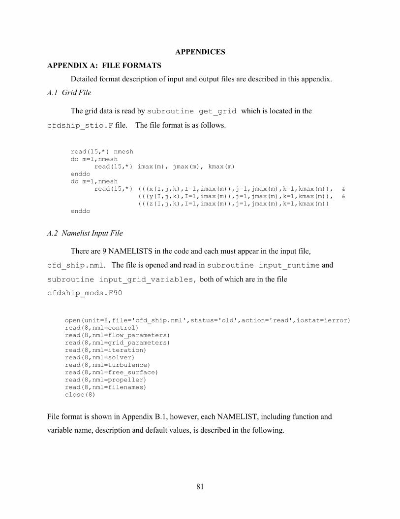
81

APPENDICES

APPENDIX A: FILE FORMATS

Detailed format description of input and output files are described in this appendix.

A.1 Grid File

The grid data is read by subroutine get_grid which is located in the

cfdship_stio.F file. The file format is as follows.

read(15,*) nmesh do m=1,nmesh read(15,*) imax(m), jmax(m), kmax(m) enddo do m=1,nmesh read(15,*) (((x(I,j,k),I=1,imax(m)),j=1,jmax(m),k=1,kmax(m)), & (((y(I,j,k),I=1,imax(m)),j=1,jmax(m),k=1,kmax(m)), & (((z(I,j,k),I=1,imax(m)),j=1,jmax(m),k=1,kmax(m)) enddo

A.2 Namelist Input File

There are 9 NAMELISTS in the code and each must appear in the input file,

cfd_ship.nml. The file is opened and read in subroutine input_runtime and

subroutine input_grid_variables, both of which are in the file

cfdship_mods.F90

open(unit=8,file='cfd_ship.nml',status='old',action='read',iostat=ierror) read(8,nml=control) read(8,nml=flow_parameters) read(8,nml=grid_parameters) read(8,nml=iteration) read(8,nml=solver) read(8,nml=turbulence) read(8,nml=free_surface) read(8,nml=propeller) read(8,nml=filenames) close(8)

File format is shown in Appendix B.1, however, each NAMELIST, including function and

variable name, description and default values, is described in the following.

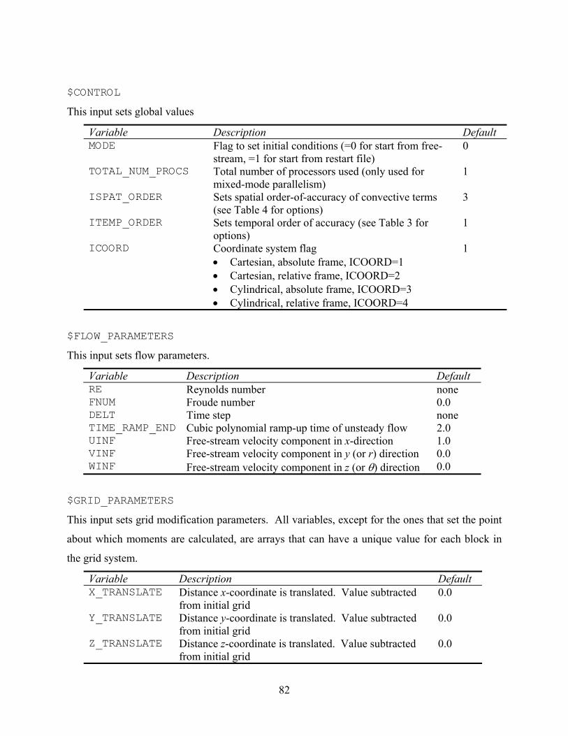
82

$CONTROL

This input sets global values

Variable Description Default MODE Flag to set initial conditions (=0 for start from free-

stream, =1 for start from restart file) 0

TOTAL_NUM_PROCS Total number of processors used (only used for mixed-mode parallelism)

1

ISPAT_ORDER Sets spatial order-of-accuracy of convective terms (see Table 4 for options)

3

ITEMP_ORDER Sets temporal order of accuracy (see Table 3 for options)

1

ICOORD Coordinate system flag • Cartesian, absolute frame, ICOORD=1 • Cartesian, relative frame, ICOORD=2 • Cylindrical, absolute frame, ICOORD=3 • Cylindrical, relative frame, ICOORD=4

1

$FLOW_PARAMETERS

This input sets flow parameters.

Variable Description Default RE Reynolds number none FNUM Froude number 0.0 DELT Time step none TIME_RAMP_END Cubic polynomial ramp-up time of unsteady flow 2.0 UINF Free-stream velocity component in x-direction 1.0 VINF Free-stream velocity component in y (or r) direction 0.0 WINF Free-stream velocity component in z (or θ) direction 0.0

$GRID_PARAMETERS

This input sets grid modification parameters. All variables, except for the ones that set the point

about which moments are calculated, are arrays that can have a unique value for each block in

the grid system.

Variable Description Default X_TRANSLATE Distance x-coordinate is translated. Value subtracted

from initial grid 0.0

Y_TRANSLATE Distance y-coordinate is translated. Value subtracted from initial grid

0.0

Z_TRANSLATE Distance z-coordinate is translated. Value subtracted from initial grid

0.0

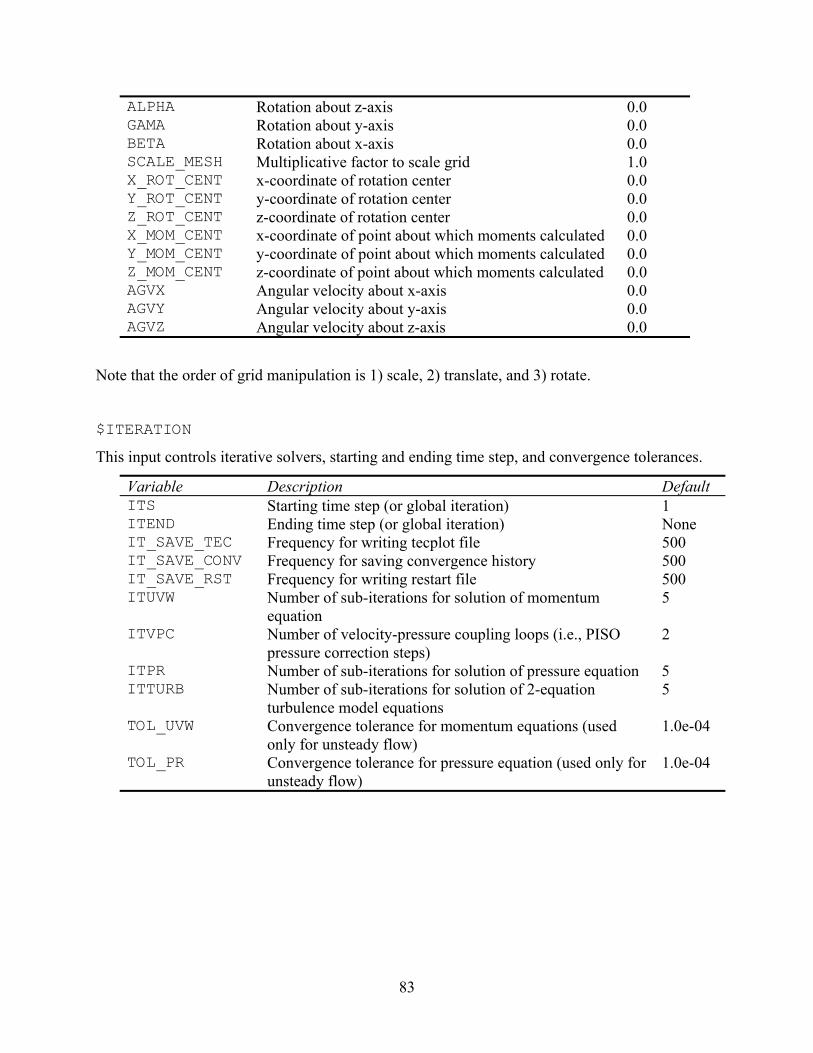
83

ALPHA Rotation about z-axis 0.0 GAMA Rotation about y-axis 0.0 BETA Rotation about x-axis 0.0 SCALE_MESH Multiplicative factor to scale grid 1.0 X_ROT_CENT x-coordinate of rotation center 0.0 Y_ROT_CENT y-coordinate of rotation center 0.0 Z_ROT_CENT z-coordinate of rotation center 0.0 X_MOM_CENT x-coordinate of point about which moments calculated 0.0 Y_MOM_CENT y-coordinate of point about which moments calculated 0.0 Z_MOM_CENT z-coordinate of point about which moments calculated 0.0 AGVX Angular velocity about x-axis 0.0 AGVY Angular velocity about y-axis 0.0 AGVZ Angular velocity about z-axis 0.0

Note that the order of grid manipulation is 1) scale, 2) translate, and 3) rotate.

$ITERATION

This input controls iterative solvers, starting and ending time step, and convergence tolerances.

Variable Description Default ITS Starting time step (or global iteration) 1 ITEND Ending time step (or global iteration) None IT_SAVE_TEC Frequency for writing tecplot file 500 IT_SAVE_CONV Frequency for saving convergence history 500 IT_SAVE_RST Frequency for writing restart file 500 ITUVW Number of sub-iterations for solution of momentum

equation 5

ITVPC Number of velocity-pressure coupling loops (i.e., PISO pressure correction steps)

2

ITPR Number of sub-iterations for solution of pressure equation 5 ITTURB Number of sub-iterations for solution of 2-equation

turbulence model equations 5

TOL_UVW Convergence tolerance for momentum equations (used only for unsteady flow)

1.0e-04

TOL_PR Convergence tolerance for pressure equation (used only for unsteady flow)

1.0e-04

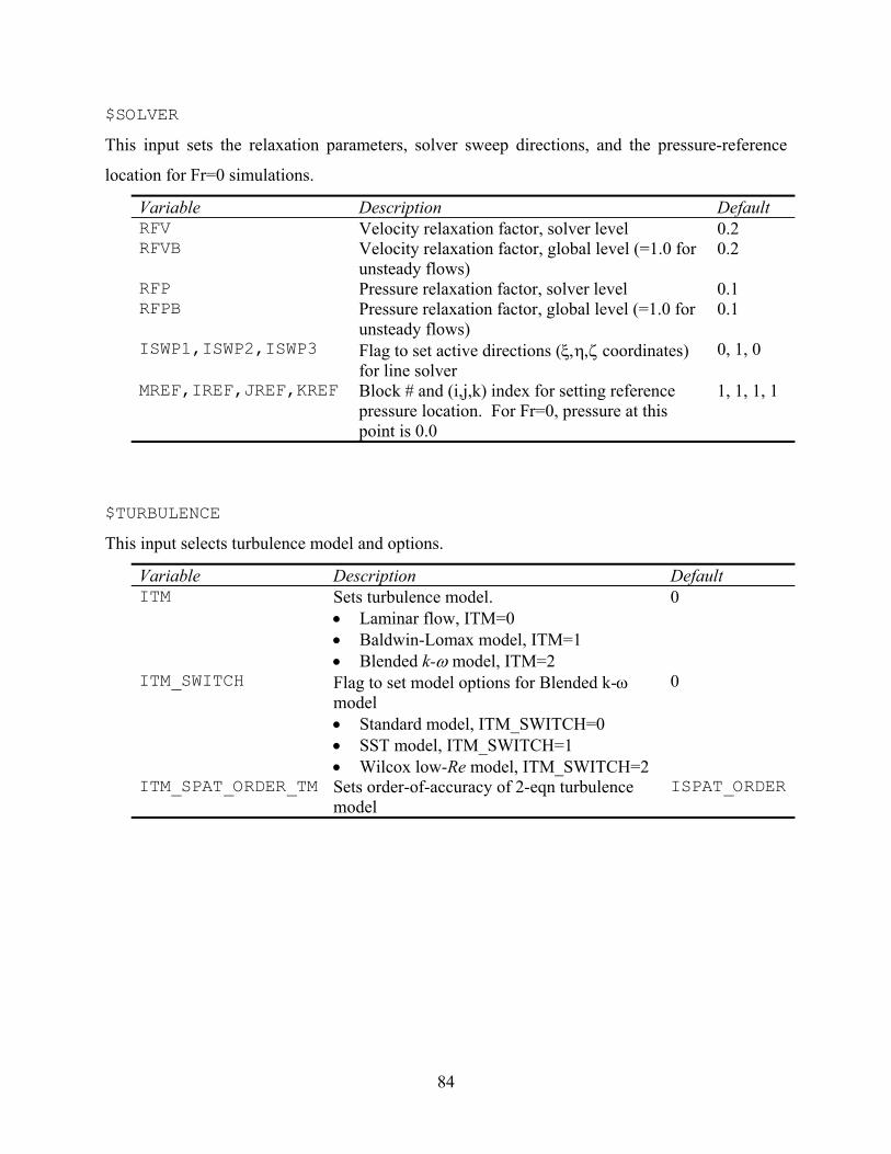
84

$SOLVER

This input sets the relaxation parameters, solver sweep directions, and the pressure-reference

location for Fr=0 simulations.

Variable Description Default RFV Velocity relaxation factor, solver level 0.2 RFVB Velocity relaxation factor, global level (=1.0 for

unsteady flows) 0.2

RFP Pressure relaxation factor, solver level 0.1 RFPB Pressure relaxation factor, global level (=1.0 for

unsteady flows) 0.1

ISWP1,ISWP2,ISWP3 Flag to set active directions (ξ,η,ζ coordinates) for line solver

0, 1, 0

MREF,IREF,JREF,KREF Block # and (i,j,k) index for setting reference pressure location. For Fr=0, pressure at this point is 0.0

1, 1, 1, 1

$TURBULENCE

This input selects turbulence model and options.

Variable Description Default ITM Sets turbulence model.

• Laminar flow, ITM=0 • Baldwin-Lomax model, ITM=1 • Blended k-ω model, ITM=2

0

ITM_SWITCH Flag to set model options for Blended k-ω model • Standard model, ITM_SWITCH=0 • SST model, ITM_SWITCH=1 • Wilcox low-Re model, ITM_SWITCH=2

0

ITM_SPAT_ORDER_TM Sets order-of-accuracy of 2-eqn turbulence model

ISPAT_ORDER

85

$FREE_SURFACE

This input sets parameters for free-surface solver and dynamic grid conforming process.

Variable Description Default ITFSMAX Number of free-surface iterations 5 TOL_FS Convergence tolerance for free-surface solution (only used for

unsteady simulations) 1.0e-04

WAVBLANK Blanking distance for near-wall region of free-surface 0.0 IFS Frequency, in global time steps, of free-surface solution 5 ICFM Flag indicating whether grid is conformed to free surface or

design waterline (z/L=0.0). ICFM=0, no conform; ICFM =1, conform turned on.

0

$PROPELLER

This input controls the prescribed body-force described in Section 2.5.

Variable Description Default IPROP number of propellers 0 CT Thrust coefficient 0.0 CKQ Torque coefficient 0.0 ADVANCE_COEF Propeller advance coefficient 0.0 DXPROP Propeller disk thickness 0.0 RP Propeller radius 0.0 X_PROP_CENTER x-coordinate of propeller center 0.0 Y_PROP_CENTER y-coordinate of propeller center 0.0 Z_PROP_CENTER z-coordinate of propeller center 0.0 RH Propeller hub radius (in decimal % of RP) 0.0 SHAFTALPHA Angle of propeller shaft with x-coordinate 0.0

$FILENAMES

This input sets the filename extensions.

Variable Description Default FGRID Variable which sets filename for grid file None FNAMEI Variable which sets “previous_simulation” filename prefix None FNAMEO Variable which sets “current_simulation” filename prefix None

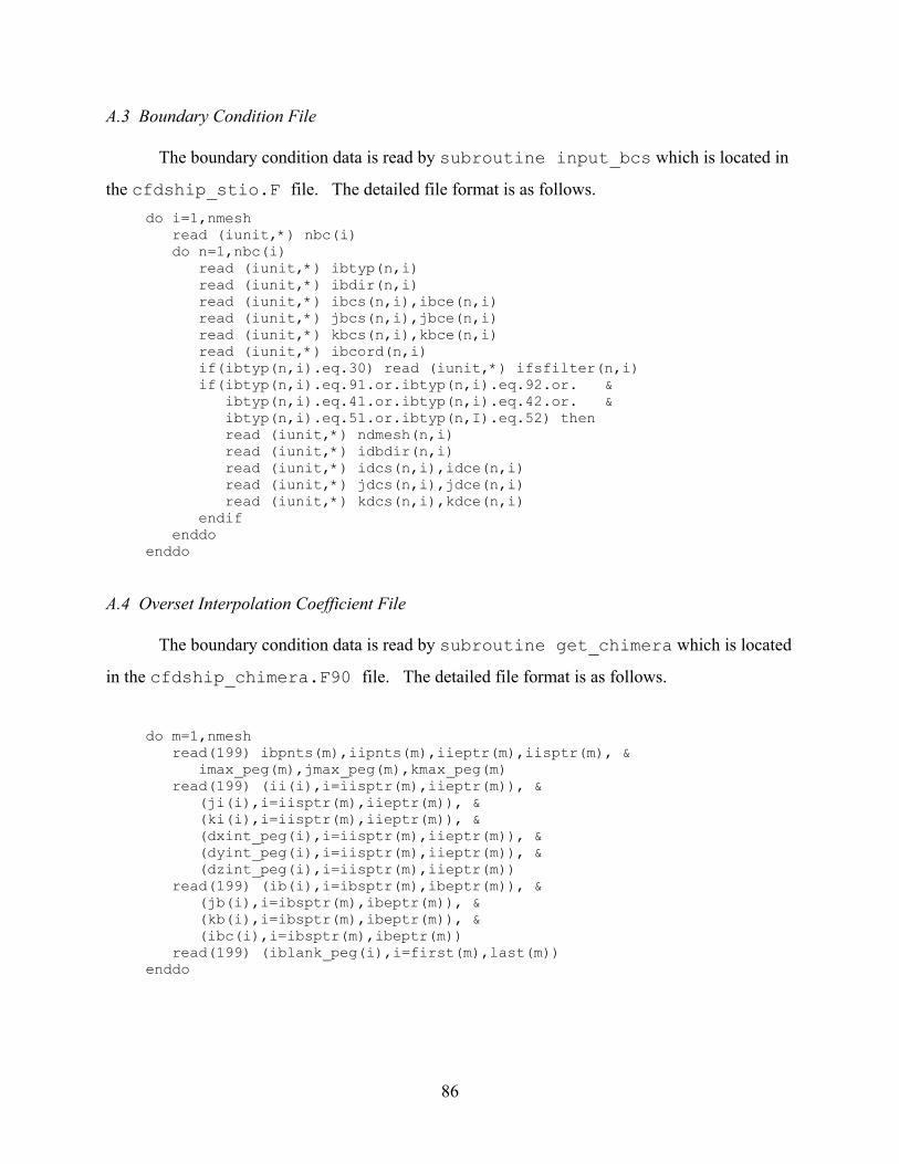
86

A.3 Boundary Condition File

The boundary condition data is read by subroutine input_bcs which is located in

the cfdship_stio.F file. The detailed file format is as follows. do i=1,nmesh read (iunit,*) nbc(i) do n=1,nbc(i) read (iunit,*) ibtyp(n,i) read (iunit,*) ibdir(n,i) read (iunit,*) ibcs(n,i),ibce(n,i) read (iunit,*) jbcs(n,i),jbce(n,i) read (iunit,*) kbcs(n,i),kbce(n,i) read (iunit,*) ibcord(n,i) if(ibtyp(n,i).eq.30) read (iunit,*) ifsfilter(n,i) if(ibtyp(n,i).eq.91.or.ibtyp(n,i).eq.92.or. & ibtyp(n,i).eq.41.or.ibtyp(n,i).eq.42.or. & ibtyp(n,i).eq.51.or.ibtyp(n,I).eq.52) then read (iunit,*) ndmesh(n,i) read (iunit,*) idbdir(n,i) read (iunit,*) idcs(n,i),idce(n,i) read (iunit,*) jdcs(n,i),jdce(n,i) read (iunit,*) kdcs(n,i),kdce(n,i) endif enddo enddo A.4 Overset Interpolation Coefficient File

The boundary condition data is read by subroutine get_chimera which is located

in the cfdship_chimera.F90 file. The detailed file format is as follows.

do m=1,nmesh read(199) ibpnts(m),iipnts(m),iieptr(m),iisptr(m), & imax_peg(m),jmax_peg(m),kmax_peg(m) read(199) (ii(i),i=iisptr(m),iieptr(m)), & (ji(i),i=iisptr(m),iieptr(m)), & (ki(i),i=iisptr(m),iieptr(m)), & (dxint_peg(i),i=iisptr(m),iieptr(m)), & (dyint_peg(i),i=iisptr(m),iieptr(m)), & (dzint_peg(i),i=iisptr(m),iieptr(m)) read(199) (ib(i),i=ibsptr(m),ibeptr(m)), & (jb(i),i=ibsptr(m),ibeptr(m)), & (kb(i),i=ibsptr(m),ibeptr(m)), & (ibc(i),i=ibsptr(m),ibeptr(m)) read(199) (iblank_peg(i),i=first(m),last(m)) enddo

87

A.5 Global Solution File

The global solution file is written by subroutine save_tec which is located in the

cfdship_stio.F file. The detailed file format is as follows.

write(26,10) write(26,20) do m=1,nmesh write(26,30) imax(m),jmax(m),kmax(m) write(26,40) (((x(i,j,k,m),i=1,imax(m)),j=1,jmax(m)),k=1,kmax(m)) write(26,40) (((y(i,j,k,m),i=1,imax(m)),j=1,jmax(m)),k=1,kmax(m)) write(26,40) (((z(i,j,k,m),i=1,imax(m)),j=1,jmax(m)),k=1,kmax(m)) write(26,40) (((u(i,j,k,m),i=1,imax(m)),j=1,jmax(m)),k=1,kmax(m)) write(26,40) (((v(i,j,k,m),i=1,imax(m)),j=1,jmax(m)),k=1,kmax(m)) write(26,40) (((w(i,j,k,m),i=1,imax(m)),j=1,jmax(m)),k=1,kmax(m)) write(26,40) (((pr(i,j,k,m),i=1,imax(m)),j=1,jmax(m)),k=1,kmax(m)) write(26,40) (((zut(i,j,k,m),i=1,imax(m)),j=1,jmax(m)),k=1,kmax(m)) write(26,40) (((yplus(i,j,k,m),i=1,imax(m)),j=1,jmax(m)),k=1,kmax(m)) write(26,40) (((uplus(i,j,k,m),i=1,imax(m)),j=1,jmax(m)),k=1,kmax(m)) write(26,41) (((iblank(i,j,k,m),i=1,imax(m)),j=1,jmax(m)),k=1,kmax(m)) write(26,40) (((ak(i,j,k,m),i=1,imax(m)),j=1,jmax(m)),k=1,kmax(m)) write(26,40) (((ao(i,j,k,m),i=1,imax(m)),j=1,jmax(m)),k=1,kmax(m)) enddo 10 format('TITLE = "TITLE STRING"') 20 format('VARIABLES = X, Y, Z, U, V, W, P, ZUT, YPLUS, UPLUS, IBLANK',', K, OMEGA') 30 format('ZONE I =',I3,', J=',I3,', K=',I3,', F=BLOCK') 40 format(6e14.6) 41 format(30i4)

A.6 Restart File

The restart file is read by subroutine get_restart and is written by

subroutine save_restart, both of which are located in the cfdship_stio.F file.

The detailed file format is as follows.

read(35) ntot_orig, nmesh do m=1,nmesh read(35) first_orig(m), last_orig(m), length_orig(m) read(35) imax_orig(m), jmax_orig(m), kmax_orig(m) enddo read(35) ((((x0(i,j,k,m),i=1,imax(m)),j=1,jmax(m)),k=1,kmax(m)),m=1,nmesh) read(35) ((((y0(i,j,k,m),i=1,imax(m)),j=1,jmax(m)),k=1,kmax(m)),m=1,nmesh) read(35) ((((z0(i,j,k,m),i=1,imax(m)),j=1,jmax(m)),k=1,kmax(m)),m=1,nmesh) read(35) ((((u0(i,j,k,m),i=1,imax(m)),j=1,jmax(m)),k=1,kmax(m)),m=1,nmesh) read(35) ((((v0(i,j,k,m),i=1,imax(m)),j=1,jmax(m)),k=1,kmax(m)),m=1,nmesh) read(35) ((((w0(i,j,k,m),i=1,imax(m)),j=1,jmax(m)),k=1,kmax(m)),m=1,nmesh) read(35) ((((pr0(i,j,k,m),i=1,imax(m)),j=1,jmax(m)),k=1,kmax(m)),m=1,nmesh) read(35) ((((zut0(i,j,k,m),i=1,imax(m)),j=1,jmax(m)),k=1,kmax(m)),m=1,nmesh)

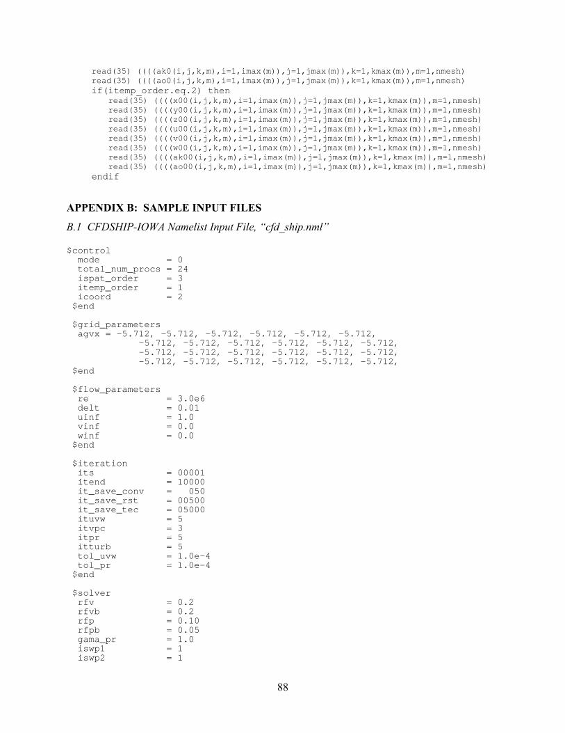
88

read(35) ((((ak0(i,j,k,m),i=1,imax(m)),j=1,jmax(m)),k=1,kmax(m)),m=1,nmesh) read(35) ((((ao0(i,j,k,m),i=1,imax(m)),j=1,jmax(m)),k=1,kmax(m)),m=1,nmesh) if(itemp_order.eq.2) then read(35) ((((x00(i,j,k,m),i=1,imax(m)),j=1,jmax(m)),k=1,kmax(m)),m=1,nmesh) read(35) ((((y00(i,j,k,m),i=1,imax(m)),j=1,jmax(m)),k=1,kmax(m)),m=1,nmesh) read(35) ((((z00(i,j,k,m),i=1,imax(m)),j=1,jmax(m)),k=1,kmax(m)),m=1,nmesh) read(35) ((((u00(i,j,k,m),i=1,imax(m)),j=1,jmax(m)),k=1,kmax(m)),m=1,nmesh) read(35) ((((v00(i,j,k,m),i=1,imax(m)),j=1,jmax(m)),k=1,kmax(m)),m=1,nmesh) read(35) ((((w00(i,j,k,m),i=1,imax(m)),j=1,jmax(m)),k=1,kmax(m)),m=1,nmesh) read(35) ((((ak00(i,j,k,m),i=1,imax(m)),j=1,jmax(m)),k=1,kmax(m)),m=1,nmesh) read(35) ((((ao00(i,j,k,m),i=1,imax(m)),j=1,jmax(m)),k=1,kmax(m)),m=1,nmesh) endif

APPENDIX B: SAMPLE INPUT FILES

B.1 CFDSHIP-IOWA Namelist Input File, “cfd_ship.nml”

$control mode = 0 total_num_procs = 24 ispat_order = 3 itemp_order = 1 icoord = 2 $end $grid_parameters agvx = -5.712, -5.712, -5.712, -5.712, -5.712, -5.712, -5.712, -5.712, -5.712, -5.712, -5.712, -5.712, -5.712, -5.712, -5.712, -5.712, -5.712, -5.712, -5.712, -5.712, -5.712, -5.712, -5.712, -5.712, $end $flow_parameters re = 3.0e6 delt = 0.01 uinf = 1.0 vinf = 0.0 winf = 0.0 $end $iteration its = 00001 itend = 10000 it_save_conv = 050 it_save_rst = 00500 it_save_tec = 05000 ituvw = 5 itvpc = 3 itpr = 5 itturb = 5 tol_uvw = 1.0e-4 tol_pr = 1.0e-4 $end $solver rfv = 0.2 rfvb = 0.2 rfp = 0.10 rfpb = 0.05 gama_pr = 1.0 iswp1 = 1 iswp2 = 1

89

iswp3 = 1 mref = 1 iref = 1 jref = 41 kref = 21 $end $turbulence itm = 2 itm_switch = 0 ispat_order_tm = 1 $end $free_surface $end $propeller $end $filenames fgrid = "p5168_14b_c1.grd" fnamei = "p5168_14b_c1" fnameo = "p5168_14b_c1" $end B.2 PEGASUS v5.1 Namelist Input File, “peg.in”

$GLOBAL FRINGE = 2, PROJECT =.T., $END $MESH NAME = 'BLK-1', KINCLUDE= 2, -1, OFFSET=1, $END $MESH NAME = 'BLK-2', KINCLUDE= 2, -1, OFFSET=1,$END $MESH NAME = 'BLK-3', KINCLUDE= 2, -1, OFFSET=1,$END $MESH NAME = 'BLK-4', KINCLUDE= 2, -1, OFFSET=1,$END $MESH NAME = 'BLK-5', KINCLUDE= 2, -1, OFFSET=1,$END $MESH NAME = 'BLK-6', KINCLUDE= 2, -1, OFFSET=1,$END $MESH NAME = 'BLK-7', KINCLUDE= 2, -1, OFFSET=1,$END $MESH NAME = 'BLK-8', KINCLUDE= 2, -1, OFFSET=1,$END $MESH NAME = 'BLK-9', KINCLUDE= 2, -1, OFFSET=1,$END $MESH NAME = 'BLK-10', KINCLUDE= 2, -1, OFFSET=1,$END $MESH NAME = 'BLK-11', KINCLUDE= 2, -1, OFFSET=1,$END $MESH NAME = 'BLK-12', KINCLUDE= 2, -1, OFFSET=1,$END $MESH NAME = 'BLK-13', KINCLUDE= 2, -1, LINCLUDE= 2, -1, $END $MESH NAME = 'BLK-14', KINCLUDE= 2, -1, LINCLUDE= 2, -1, $END $MESH NAME = 'BLK-15', KINCLUDE= 2, -1, LINCLUDE= 2, -1, $END $MESH NAME = 'BLK-16', KINCLUDE= 2, -1, LINCLUDE= 2, -1, $END

90

$MESH NAME = 'BLK-17', KINCLUDE= 2, -1, LINCLUDE= 2, -1, $END $MESH NAME = 'BLK-18', KINCLUDE= 2, -1, LINCLUDE= 2, -1, $END $MESH NAME = 'BLK-19', KINCLUDE= 2, -1, PHANTOM=.T.,$END $HCUT NAME = 'blade_cutter', INTERNAL=.F., MEMBER = 'BLK-19', 'BLK-5','BLK-6','BLK-7','BLK-8','BLK-9','BLK-10','BLK-11', 'BLK-12','BLK-13','BLK-14','BLK-15','BLK-16','BLK-17','BLK-18', INCLUDE = 'BLK-1','BLK-2','BLK-3','BLK-4', CARTX=-81.6, 81.6, $END $HCUT NAME = 'passage_cutter', INTERNAL=.T., MEMBER = 'BLK-1','BLK-2','BLK-3','BLK-4', INCLUDE = 'BLK-5','BLK-6','BLK-7','BLK-8','BLK-9','BLK-10','BLK-11', 'BLK-12','BLK-13','BLK-14','BLK-15','BLK-16','BLK-17','BLK-18', $END $LEVEL2 EXCLUDE='BLK-1','BLK-2','BLK-3','BLK-4', $END $BCINP ISPARTOF = 'BLK-1', IBTYP = 5, 40, 5, 5, 5, 5, IBDIR = 3, -1, -3, 2, 1, -2, JBCS = 1, 61, 1, 1, 1, 1, JBCE = 61, 61, 61, 61, 1, 61, KBCS = 1, 1, 1, 1, 1, 81, KBCE = 81, 81, 81, 1, 81, 81, LBCS = 1, 1, 81, 1, 1, 1, LBCE = 1, 81, 81, 81, 81, 81, $END $BCINP ISPARTOF = 'BLK-2', IBTYP = 5, 5, 40, 5, 40, 5, IBDIR = 2, 3, -1, -3, 1, -2, JBCS = 1, 1, 61, 1, 1, 1, JBCE = 61, 61, 61, 61, 1, 61, KBCS = 1, 1, 1, 1, 1, 81, KBCE = 1, 81, 81, 81, 81, 81, LBCS = 1, 1, 1, 81, 1, 1, LBCE = 81, 1, 81, 81, 81, 81, $END $BCINP ISPARTOF = 'BLK-3', IBTYP = 5, 5, 5, 40, 40, 5, IBDIR = 2, 3, -3, -1, 1, -2, JBCS = 1, 1, 1, 61, 1, 1, JBCE = 61, 61, 61, 61, 1, 61, KBCS = 1, 1, 1, 1, 1, 81, KBCE = 1, 81, 81, 81, 81, 81, LBCS = 1, 1, 81, 1, 1, 1, LBCE = 81, 1, 81, 81, 81, 81, $END $BCINP ISPARTOF = 'BLK-4', IBTYP = 5, 5, 5, 40, 5, 5, IBDIR = 2, -1, 3, 1, -3, -2, JBCS = 1, 61, 1, 1, 1, 1, JBCE = 61, 61, 61, 1, 61, 61,

91

KBCS = 1, 1, 1, 1, 1, 81, KBCE = 1, 81, 81, 81, 81, 81, LBCS = 1, 1, 1, 1, 81, 1, LBCE = 81, 81, 1, 81, 81, 81, $END $BCINP ISPARTOF = 'BLK-5', IBTYP = 5, IBDIR = 2, JBCS = 1, JBCE = 41, KBCS = 1, KBCE = 1, LBCS = 1, LBCE = 31, $END $BCINP ISPARTOF = 'BLK-6', IBTYP = 5, IBDIR = 2, JBCS = 1, JBCE = 41, KBCS = 1, KBCE = 1, LBCS = 1, LBCE = 31, $END $BCINP ISPARTOF = 'BLK-7', IBTYP = 5, 40, 40, 40, IBDIR = 2, 1, 3, -3, JBCS = 1, 1, 1, 1, JBCE = 45, 1, 45, 45, KBCS = 1, 1, 1, 1, KBCE = 1, 61, 61, 61, LBCS = 1, 1, 1, 31, LBCE = 31, 31, 1, 31, $END $BCINP ISPARTOF = 'BLK-8', IBTYP = 5, 40, 40, 40, IBDIR = 2, -1, 3, -3, JBCS = 1, 45, 1, 1, JBCE = 45, 45, 45, 45, KBCS = 1, 1, 1, 1, KBCE = 1, 61, 61, 61, LBCS = 1, 1, 1, 31, LBCE = 31, 31, 1, 31, $END $BCINP ISPARTOF = 'BLK-9', IBTYP = 5, 40, 40, 40, IBDIR = 2, -1, -3, 3, JBCS = 1, 45, 1, 1, JBCE = 45, 45, 45, 45, KBCS = 1, 1, 1, 1, KBCE = 1, 61, 61, 61, LBCS = 1, 1, 31, 1, LBCE = 31, 31, 31, 1, $END $BCINP ISPARTOF = 'BLK-10', IBTYP = 5, 40, 40, 40, IBDIR = 2, 1, -3, 3,

92

JBCS = 1, 1, 1, 1, JBCE = 45, 1, 45, 45, KBCS = 1, 1, 1, 1, KBCE = 1, 61, 61, 61, LBCS = 1, 1, 31, 1, LBCE = 31, 31, 31, 1, $END $BCINP ISPARTOF = 'BLK-11', IBTYP = 5, 40, 40, 40, 40, IBDIR = 2, -3, -3, 1, -1, JBCS = 1, 1, 25, 1, 41, JBCE = 41, 25, 41, 1, 41, KBCS = 1, 1, 1, 1, 1, KBCE = 1, 61, 61, 61, 61, LBCS = 1, 45, 45, 1, 1, LBCE = 45, 45, 45, 45, 45, $END $BCINP ISPARTOF = 'BLK-12', IBTYP = 5, 40, 40, 40, 40, IBDIR = 2, -3, -3, -1, 1, JBCS = 1, 17, 1, 41, 1, JBCE = 41, 41, 17, 41, 1, KBCS = 1, 1, 1, 1, 1, KBCE = 1, 61, 61, 61, 61, LBCS = 1, 45, 45, 1, 1, LBCE = 45, 45, 45, 45, 45, $END $BCINP ISPARTOF = 'BLK-13', IBTYP = 5, 5, 40, 40, 40, 40, IBDIR = 2, 2, -1, -3, 1, 3, JBCS = 1, 1, 45, 1, 1, 1, JBCE = 45, 45, 45, 45, 1, 45, KBCS = 1, 1, 1, 1, 1, 1, KBCE = 1, 1, 61, 61, 61, 61, LBCS = 51, 1, 1, 65, 1, 1, LBCE = 65, 51, 65, 65, 65, 1, $END $BCINP ISPARTOF = 'BLK-14', IBTYP = 5, 5, 40, 40, 40, IBDIR = 2, 2, -1, 1, 3, JBCS = 1, 1, 41, 1, 1, JBCE = 41, 41, 41, 1, 41, KBCS = 1, 1, 1, 1, 1, KBCE = 1, 1, 61, 61, 61, LBCS = 51, 1, 1, 1, 1, LBCE = 65, 51, 65, 65, 1, $END $BCINP ISPARTOF = 'BLK-15', IBTYP = 5, 5, 40, 40, 40, 40, IBDIR = 2, 2, -1, -3, 1, 3, JBCS = 1, 1, 45, 1, 1, 1, JBCE = 45, 45, 45, 45, 1, 45, KBCS = 1, 1, 1, 1, 1, 1, KBCE = 1, 1, 61, 61, 61, 61, LBCS = 51, 1, 1, 65, 1, 1, LBCE = 65, 51, 65, 65, 65, 1, $END $BCINP ISPARTOF = 'BLK-16',

93

IBTYP = 40, 5, 5, 40, 40, 40, IBDIR = 3, 2, 2, 1, -1, -3, JBCS = 1, 1, 1, 1, 45, 1, JBCE = 45, 45, 45, 1, 45, 45, KBCS = 1, 1, 1, 1, 1, 1, KBCE = 61, 1, 1, 61, 61, 61, LBCS = 1, 51, 1, 1, 1, 65, LBCE = 1, 65, 51, 65, 65, 65, $END $BCINP ISPARTOF = 'BLK-17', IBTYP = 40, 5, 5, 40, 40, IBDIR = 3, 2, 2, 1, -1, JBCS = 1, 1, 1, 1, 41, JBCE = 41, 41, 41, 1, 41, KBCS = 1, 1, 1, 1, 1, KBCE = 61, 1, 1, 61, 61, LBCS = 1, 1, 51, 1, 1, LBCE = 1, 51, 65, 65, 65, $END $BCINP ISPARTOF = 'BLK-18', IBTYP = 40, 5, 5, 40, 40, 40, IBDIR = 3, 2, 2, 1, -1, -3, JBCS = 1, 1, 1, 1, 45, 1, JBCE = 45, 45, 45, 1, 45, 45, KBCS = 1, 1, 1, 1, 1, 1, KBCE = 61, 1, 1, 61, 61, 61, LBCS = 1, 1, 51, 1, 1, 65, LBCE = 1, 51, 65, 65, 65, 65, $END $BCINP ISPARTOF = 'BLK-19', IBTYP = 5, IBDIR = 2, JBCS = 1, JBCE = -1, KBCS = 1, KBCE = 1, LBCS = 1, LBCE = -1, $END B.3 Boundary condition file

6 ! number of boundary surfaces ===> BLK#-1 52 !*** periodic MB #1= type #52 3 ! coordinate direction normal to surface 1 61 ! start, end in i-direction 1 81 ! start, end in j-direction 1 1 ! start, end in k-direction 1 ! flag for order of first derivative bc 1 ! donor mesh -3 ! coordinate direction normal to surface 1 61 ! donor mesh start, end in i-direction 1 81 ! donor mesh start, end in j-direction 81 81 ! donor mesh start, end in k-direction 92 !*** patched MB #2= type #92 -1 ! coordinate direction normal to surface 61 61 ! start, end in i-direction 1 81 ! start, end in j-direction 1 81 ! start, end in k-direction 1 ! flag for order of first derivative bc 2 ! donor mesh

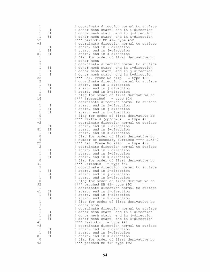
94

1 ! coordinate direction normal to surface 1 1 ! donor mesh start, end in i-direction 1 81 ! donor mesh start, end in j-direction 1 81 ! donor mesh start, end in k-direction 52 !*** periodic MB #1= type #52 -3 ! coordinate direction normal to surface 1 61 ! start, end in i-direction 1 81 ! start, end in j-direction 81 81 ! start, end in k-direction 1 ! flag for order of first derivative bc 1 ! donor mesh 3 ! coordinate direction normal to surface 1 61 ! donor mesh start, end in i-direction 1 81 ! donor mesh start, end in j-direction 1 1 ! donor mesh start, end in k-direction 22 !*** Rel. Frame No-slip = type #22 2 ! coordinate direction normal to surface 1 61 ! start, end in i-direction 1 1 ! start, end in j-direction 1 81 ! start, end in k-direction 0 ! flag for order of first derivative bc 14 !*** Prescribed = type #14 1 ! coordinate direction normal to surface 1 1 ! start, end in i-direction 1 81 ! start, end in j-direction 1 81 ! start, end in k-direction 0 ! flag for order of first derivative bc 13 !*** Farfield (dp/dn=0) = type #13 -2 ! coordinate direction normal to surface 1 61 ! start, end in i-direction 81 81 ! start, end in j-direction 1 81 ! start, end in k-direction 0 ! flag for order of first derivative bc 6 ! number of boundary surfaces ===> BLK#-2 22 !*** Rel. Frame No-slip = type #22 2 ! coordinate direction normal to surface 1 61 ! start, end in i-direction 1 1 ! start, end in j-direction 1 81 ! start, end in k-direction 0 ! flag for order of first derivative bc 41 !*** Periodic = type #41 3 ! coordinate direction normal to surface 1 61 ! start, end in i-direction 1 81 ! start, end in j-direction 1 1 ! start, end in k-direction 0 ! flag for order of first derivative bc 92 !*** patched MB #3= type #92 -1 ! coordinate direction normal to surface 61 61 ! start, end in i-direction 1 81 ! start, end in j-direction 1 81 ! start, end in k-direction 1 ! flag for order of first derivative bc 3 ! donor mesh 1 ! coordinate direction normal to surface 1 1 ! donor mesh start, end in i-direction 1 81 ! donor mesh start, end in j-direction 1 81 ! donor mesh start, end in k-direction 41 !*** Periodic = type #41 -3 ! coordinate direction normal to surface 1 61 ! start, end in i-direction 1 81 ! start, end in j-direction 81 81 ! start, end in k-direction 0 ! flag for order of first derivative bc 92 !*** patched MB #1= type #92

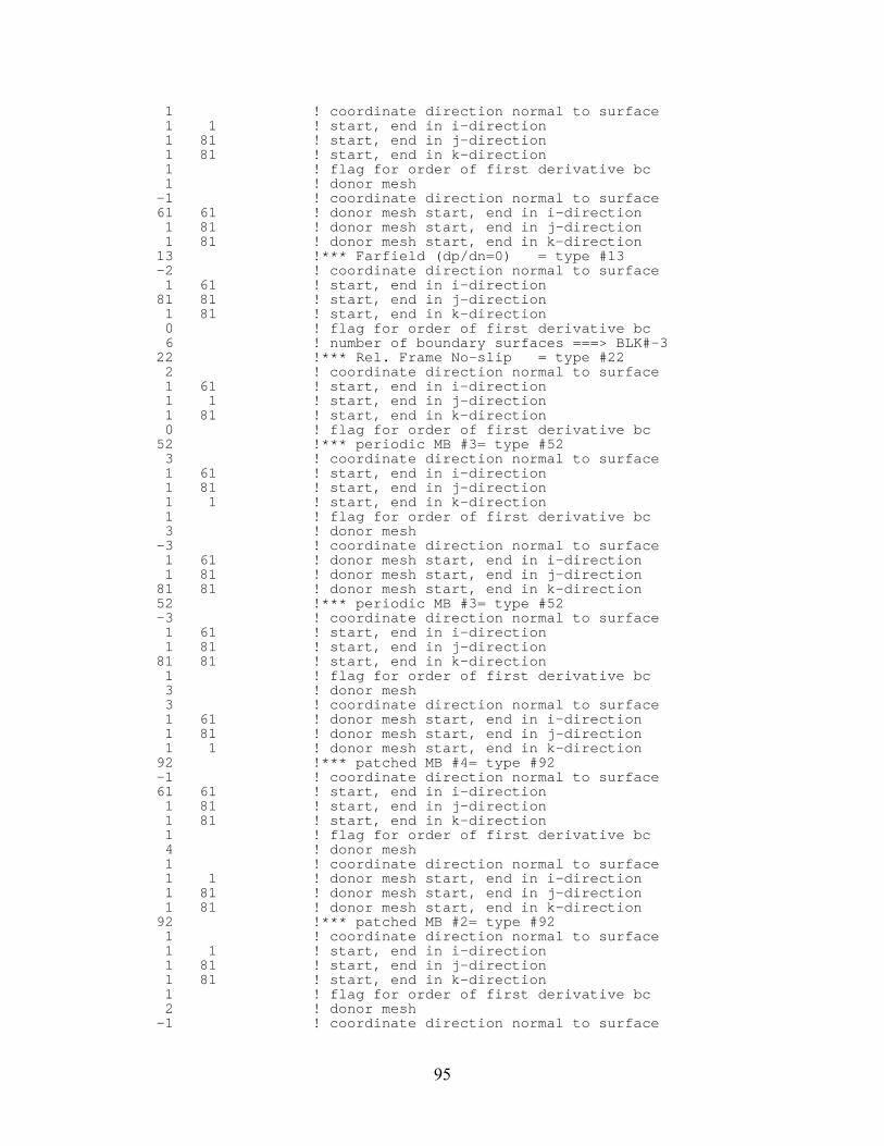
95

1 ! coordinate direction normal to surface 1 1 ! start, end in i-direction 1 81 ! start, end in j-direction 1 81 ! start, end in k-direction 1 ! flag for order of first derivative bc 1 ! donor mesh -1 ! coordinate direction normal to surface 61 61 ! donor mesh start, end in i-direction 1 81 ! donor mesh start, end in j-direction 1 81 ! donor mesh start, end in k-direction 13 !*** Farfield (dp/dn=0) = type #13 -2 ! coordinate direction normal to surface 1 61 ! start, end in i-direction 81 81 ! start, end in j-direction 1 81 ! start, end in k-direction 0 ! flag for order of first derivative bc 6 ! number of boundary surfaces ===> BLK#-3 22 !*** Rel. Frame No-slip = type #22 2 ! coordinate direction normal to surface 1 61 ! start, end in i-direction 1 1 ! start, end in j-direction 1 81 ! start, end in k-direction 0 ! flag for order of first derivative bc 52 !*** periodic MB #3= type #52 3 ! coordinate direction normal to surface 1 61 ! start, end in i-direction 1 81 ! start, end in j-direction 1 1 ! start, end in k-direction 1 ! flag for order of first derivative bc 3 ! donor mesh -3 ! coordinate direction normal to surface 1 61 ! donor mesh start, end in i-direction 1 81 ! donor mesh start, end in j-direction 81 81 ! donor mesh start, end in k-direction 52 !*** periodic MB #3= type #52 -3 ! coordinate direction normal to surface 1 61 ! start, end in i-direction 1 81 ! start, end in j-direction 81 81 ! start, end in k-direction 1 ! flag for order of first derivative bc 3 ! donor mesh 3 ! coordinate direction normal to surface 1 61 ! donor mesh start, end in i-direction 1 81 ! donor mesh start, end in j-direction 1 1 ! donor mesh start, end in k-direction 92 !*** patched MB #4= type #92 -1 ! coordinate direction normal to surface 61 61 ! start, end in i-direction 1 81 ! start, end in j-direction 1 81 ! start, end in k-direction 1 ! flag for order of first derivative bc 4 ! donor mesh 1 ! coordinate direction normal to surface 1 1 ! donor mesh start, end in i-direction 1 81 ! donor mesh start, end in j-direction 1 81 ! donor mesh start, end in k-direction 92 !*** patched MB #2= type #92 1 ! coordinate direction normal to surface 1 1 ! start, end in i-direction 1 81 ! start, end in j-direction 1 81 ! start, end in k-direction 1 ! flag for order of first derivative bc 2 ! donor mesh -1 ! coordinate direction normal to surface

96

61 61 ! donor mesh start, end in i-direction 1 81 ! donor mesh start, end in j-direction 1 81 ! donor mesh start, end in k-direction 13 !*** Farfield (dp/dn=0) = type #13 -2 ! coordinate direction normal to surface 1 61 ! start, end in i-direction 81 81 ! start, end in j-direction 1 81 ! start, end in k-direction 0 ! flag for order of first derivative bc 6 ! number of boundary surfaces ===> BLK#-4 22 !*** Rel. Frame No-slip = type #22 2 ! coordinate direction normal to surface 1 61 ! start, end in i-direction 1 1 ! start, end in j-direction 1 81 ! start, end in k-direction 0 ! flag for order of first derivative bc 11 !*** Exit = type #11 -1 ! coordinate direction normal to surface 61 61 ! start, end in i-direction 1 81 ! start, end in j-direction 1 81 ! start, end in k-direction 0 ! flag for order of first derivative bc 41 !*** Periodic = type #41 3 ! coordinate direction normal to surface 1 61 ! start, end in i-direction 1 81 ! start, end in j-direction 1 1 ! start, end in k-direction 0 ! flag for order of first derivative bc 92 !*** patched MB #3= type #92 1 ! coordinate direction normal to surface 1 1 ! start, end in i-direction 1 81 ! start, end in j-direction 1 81 ! start, end in k-direction 1 ! flag for order of first derivative bc 3 ! donor mesh -1 ! coordinate direction normal to surface 61 61 ! donor mesh start, end in i-direction 1 81 ! donor mesh start, end in j-direction 1 81 ! donor mesh start, end in k-direction 41 !*** Periodic = type #41 -3 ! coordinate direction normal to surface 1 61 ! start, end in i-direction 1 81 ! start, end in j-direction 81 81 ! start, end in k-direction 0 ! flag for order of first derivative bc 13 !*** Farfield (dp/dn=0) = type #13 -2 ! coordinate direction normal to surface 1 61 ! start, end in i-direction 81 81 ! start, end in j-direction 1 81 ! start, end in k-direction 0 ! flag for order of first derivative bc 1 ! number of boundary surfaces ===> BLK#-5 22 !*** Rel. Frame No-slip = type #22 2 ! coordinate direction normal to surface 1 41 ! start, end in i-direction 1 1 ! start, end in j-direction 1 31 ! start, end in k-direction 0 ! flag for order of first derivative bc 1 ! number of boundary surfaces ===> BLK#-6 22 !*** Rel. Frame No-slip = type #22 2 ! coordinate direction normal to surface 1 41 ! start, end in i-direction 1 1 ! start, end in j-direction 1 31 ! start, end in k-direction

97

0 ! flag for order of first derivative bc 4 ! number of boundary surfaces ===> BLK#-7 22 !*** Rel. Frame No-slip = type #22 2 ! coordinate direction normal to surface 1 45 ! start, end in i-direction 1 1 ! start, end in j-direction 1 31 ! start, end in k-direction 0 ! flag for order of first derivative bc 92 !*** patched MB #8= type #92 1 ! coordinate direction normal to surface 1 1 ! start, end in i-direction 1 61 ! start, end in j-direction 1 31 ! start, end in k-direction 1 ! flag for order of first derivative bc 8 ! donor mesh -1 ! coordinate direction normal to surface 45 45 ! donor mesh start, end in i-direction 1 61 ! donor mesh start, end in j-direction 1 31 ! donor mesh start, end in k-direction 92 !*** patched MB #16= type #92 3 ! coordinate direction normal to surface 1 45 ! start, end in i-direction 1 61 ! start, end in j-direction 1 1 ! start, end in k-direction 1 ! flag for order of first derivative bc 16 ! donor mesh -3 ! coordinate direction normal to surface 1 45 ! donor mesh start, end in i-direction 1 61 ! donor mesh start, end in j-direction 65 65 ! donor mesh start, end in k-direction 92 !*** patched MB #11= type #92 -3 ! coordinate direction normal to surface 1 45 ! start, end in i-direction 1 61 ! start, end in j-direction 31 31 ! start, end in k-direction 1 ! flag for order of first derivative bc 11 ! donor mesh 1 ! coordinate direction normal to surface 1 1 ! donor mesh start, end in i-direction 1 61 ! donor mesh start, end in j-direction 45 1 ! donor mesh start, end in k-direction 4 ! number of boundary surfaces ===> BLK#-8 22 !*** Rel. Frame No-slip = type #22 2 ! coordinate direction normal to surface 1 45 ! start, end in i-direction 1 1 ! start, end in j-direction 1 31 ! start, end in k-direction 0 ! flag for order of first derivative bc 92 !*** patched MB #7= type #92 -1 ! coordinate direction normal to surface 45 45 ! start, end in i-direction 1 61 ! start, end in j-direction 1 31 ! start, end in k-direction 1 ! flag for order of first derivative bc 7 ! donor mesh 1 ! coordinate direction normal to surface 1 1 ! donor mesh start, end in i-direction 1 61 ! donor mesh start, end in j-direction 1 31 ! donor mesh start, end in k-direction 92 !*** patched MB #15= type #92 3 ! coordinate direction normal to surface 1 45 ! start, end in i-direction 1 61 ! start, end in j-direction 1 1 ! start, end in k-direction

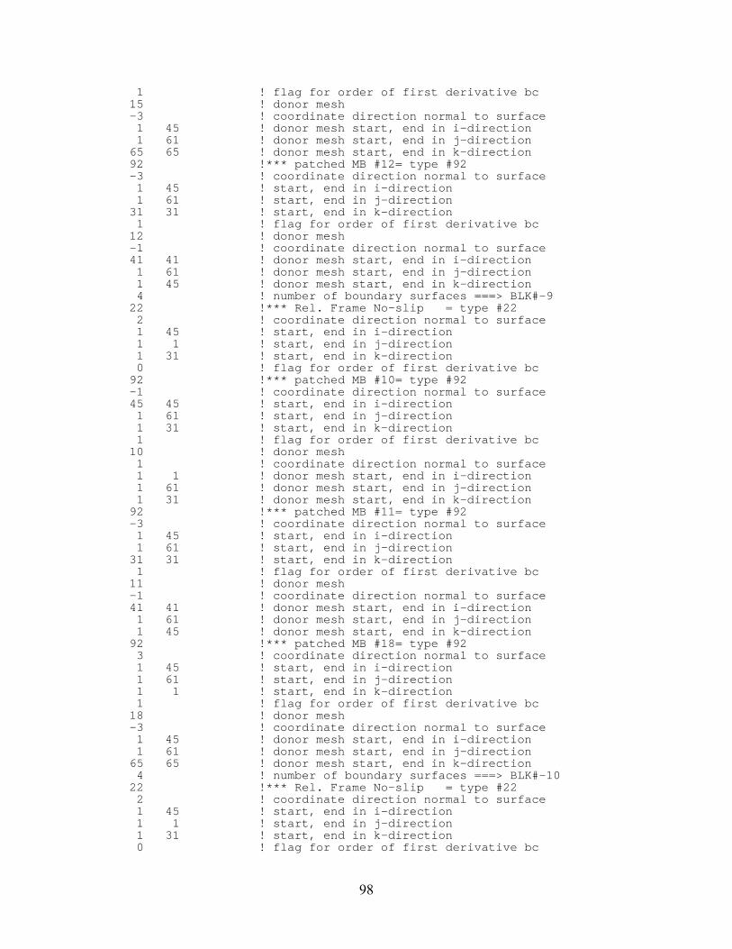
98

1 ! flag for order of first derivative bc 15 ! donor mesh -3 ! coordinate direction normal to surface 1 45 ! donor mesh start, end in i-direction 1 61 ! donor mesh start, end in j-direction 65 65 ! donor mesh start, end in k-direction 92 !*** patched MB #12= type #92 -3 ! coordinate direction normal to surface 1 45 ! start, end in i-direction 1 61 ! start, end in j-direction 31 31 ! start, end in k-direction 1 ! flag for order of first derivative bc 12 ! donor mesh -1 ! coordinate direction normal to surface 41 41 ! donor mesh start, end in i-direction 1 61 ! donor mesh start, end in j-direction 1 45 ! donor mesh start, end in k-direction 4 ! number of boundary surfaces ===> BLK#-9 22 !*** Rel. Frame No-slip = type #22 2 ! coordinate direction normal to surface 1 45 ! start, end in i-direction 1 1 ! start, end in j-direction 1 31 ! start, end in k-direction 0 ! flag for order of first derivative bc 92 !*** patched MB #10= type #92 -1 ! coordinate direction normal to surface 45 45 ! start, end in i-direction 1 61 ! start, end in j-direction 1 31 ! start, end in k-direction 1 ! flag for order of first derivative bc 10 ! donor mesh 1 ! coordinate direction normal to surface 1 1 ! donor mesh start, end in i-direction 1 61 ! donor mesh start, end in j-direction 1 31 ! donor mesh start, end in k-direction 92 !*** patched MB #11= type #92 -3 ! coordinate direction normal to surface 1 45 ! start, end in i-direction 1 61 ! start, end in j-direction 31 31 ! start, end in k-direction 1 ! flag for order of first derivative bc 11 ! donor mesh -1 ! coordinate direction normal to surface 41 41 ! donor mesh start, end in i-direction 1 61 ! donor mesh start, end in j-direction 1 45 ! donor mesh start, end in k-direction 92 !*** patched MB #18= type #92 3 ! coordinate direction normal to surface 1 45 ! start, end in i-direction 1 61 ! start, end in j-direction 1 1 ! start, end in k-direction 1 ! flag for order of first derivative bc 18 ! donor mesh -3 ! coordinate direction normal to surface 1 45 ! donor mesh start, end in i-direction 1 61 ! donor mesh start, end in j-direction 65 65 ! donor mesh start, end in k-direction 4 ! number of boundary surfaces ===> BLK#-10 22 !*** Rel. Frame No-slip = type #22 2 ! coordinate direction normal to surface 1 45 ! start, end in i-direction 1 1 ! start, end in j-direction 1 31 ! start, end in k-direction 0 ! flag for order of first derivative bc

99

92 !*** patched MB #9= type #92 1 ! coordinate direction normal to surface 1 1 ! start, end in i-direction 1 61 ! start, end in j-direction 1 31 ! start, end in k-direction 1 ! flag for order of first derivative bc 9 ! donor mesh -1 ! coordinate direction normal to surface 45 45 ! donor mesh start, end in i-direction 1 61 ! donor mesh start, end in j-direction 1 31 ! donor mesh start, end in k-direction 92 !*** patched MB #12= type #92 -3 ! coordinate direction normal to surface 1 45 ! start, end in i-direction 1 61 ! start, end in j-direction 31 31 ! start, end in k-direction 1 ! flag for order of first derivative bc 12 ! donor mesh 1 ! coordinate direction normal to surface 1 1 ! donor mesh start, end in i-direction 1 61 ! donor mesh start, end in j-direction 45 1 ! donor mesh start, end in k-direction 92 !*** patched MB #13= type #92 3 ! coordinate direction normal to surface 1 45 ! start, end in i-direction 1 61 ! start, end in j-direction 1 1 ! start, end in k-direction 1 ! flag for order of first derivative bc 13 ! donor mesh -3 ! coordinate direction normal to surface 1 45 ! donor mesh start, end in i-direction 1 61 ! donor mesh start, end in j-direction 65 65 ! donor mesh start, end in k-direction 5 ! number of boundary surfaces ===> BLK#-11 22 !*** Rel. Frame No-slip = type #22 2 ! coordinate direction normal to surface 1 41 ! start, end in i-direction 1 1 ! start, end in j-direction 1 45 ! start, end in k-direction 0 ! flag for order of first derivative bc 92 !*** patched MB #12= type #92 -3 ! coordinate direction normal to surface 1 25 ! start, end in i-direction 1 61 ! start, end in j-direction 45 45 ! start, end in k-direction 1 ! flag for order of first derivative bc 12 ! donor mesh -3 ! coordinate direction normal to surface 41 17 ! donor mesh start, end in i-direction 1 61 ! donor mesh start, end in j-direction 45 45 ! donor mesh start, end in k-direction 92 !*** patched MB #12= type #92 -3 ! coordinate direction normal to surface 25 41 ! start, end in i-direction 1 61 ! start, end in j-direction 45 45 ! start, end in k-direction 1 ! flag for order of first derivative bc 12 ! donor mesh -3 ! coordinate direction normal to surface 17 1 ! donor mesh start, end in i-direction 1 61 ! donor mesh start, end in j-direction 45 45 ! donor mesh start, end in k-direction 92 !*** patched MB #7= type #92 1 ! coordinate direction normal to surface

100

1 1 ! start, end in i-direction 1 61 ! start, end in j-direction 1 45 ! start, end in k-direction 1 ! flag for order of first derivative bc 7 ! donor mesh -3 ! coordinate direction normal to surface 45 1 ! donor mesh start, end in i-direction 1 61 ! donor mesh start, end in j-direction 31 31 ! donor mesh start, end in k-direction 92 !*** patched MB #9= type #92 -1 ! coordinate direction normal to surface 41 41 ! start, end in i-direction 1 61 ! start, end in j-direction 1 45 ! start, end in k-direction 1 ! flag for order of first derivative bc 9 ! donor mesh -3 ! coordinate direction normal to surface 1 45 ! donor mesh start, end in i-direction 1 61 ! donor mesh start, end in j-direction 31 31 ! donor mesh start, end in k-direction 5 ! number of boundary surfaces ===> BLK#-12 22 !*** Rel. Frame No-slip = type #22 2 ! coordinate direction normal to surface 1 41 ! start, end in i-direction 1 1 ! start, end in j-direction 1 45 ! start, end in k-direction 0 ! flag for order of first derivative bc 92 !*** patched MB #11= type #92 -3 ! coordinate direction normal to surface 17 41 ! start, end in i-direction 1 61 ! start, end in j-direction 45 45 ! start, end in k-direction 1 ! flag for order of first derivative bc 11 ! donor mesh -3 ! coordinate direction normal to surface 25 1 ! donor mesh start, end in i-direction 1 61 ! donor mesh start, end in j-direction 45 45 ! donor mesh start, end in k-direction 92 !*** patched MB #11= type #92 -3 ! coordinate direction normal to surface 1 17 ! start, end in i-direction 1 61 ! start, end in j-direction 45 45 ! start, end in k-direction 1 ! flag for order of first derivative bc 11 ! donor mesh -3 ! coordinate direction normal to surface 41 25 ! donor mesh start, end in i-direction 1 61 ! donor mesh start, end in j-direction 45 45 ! donor mesh start, end in k-direction 92 !*** patched MB #8= type #92 -1 ! coordinate direction normal to surface 41 41 ! start, end in i-direction 1 61 ! start, end in j-direction 1 45 ! start, end in k-direction 1 ! flag for order of first derivative bc 8 ! donor mesh -3 ! coordinate direction normal to surface 1 45 ! donor mesh start, end in i-direction 1 61 ! donor mesh start, end in j-direction 31 31 ! donor mesh start, end in k-direction 92 !*** patched MB #10= type #92 1 ! coordinate direction normal to surface 1 1 ! start, end in i-direction 1 61 ! start, end in j-direction

101

1 45 ! start, end in k-direction 1 ! flag for order of first derivative bc 10 ! donor mesh -3 ! coordinate direction normal to surface 45 1 ! donor mesh start, end in i-direction 1 61 ! donor mesh start, end in j-direction 31 31 ! donor mesh start, end in k-direction 6 ! number of boundary surfaces ===> BLK#-13 22 !*** Rel. Frame No-slip = type #22 2 ! coordinate direction normal to surface 1 45 ! start, end in i-direction 1 1 ! start, end in j-direction 51 65 ! start, end in k-direction 0 ! flag for order of first derivative bc 22 !*** Rel. Frame No-slip = type #22 2 ! coordinate direction normal to surface 1 45 ! start, end in i-direction 1 1 ! start, end in j-direction 1 51 ! start, end in k-direction 0 ! flag for order of first derivative bc 92 !*** patched MB #14= type #92 -1 ! coordinate direction normal to surface 45 45 ! start, end in i-direction 1 61 ! start, end in j-direction 1 65 ! start, end in k-direction 1 ! flag for order of first derivative bc 14 ! donor mesh 1 ! coordinate direction normal to surface 1 1 ! donor mesh start, end in i-direction 1 61 ! donor mesh start, end in j-direction 1 65 ! donor mesh start, end in k-direction 92 !*** patched MB #10= type #92 -3 ! coordinate direction normal to surface 1 45 ! start, end in i-direction 1 61 ! start, end in j-direction 65 65 ! start, end in k-direction 1 ! flag for order of first derivative bc 10 ! donor mesh 3 ! coordinate direction normal to surface 1 45 ! donor mesh start, end in i-direction 1 61 ! donor mesh start, end in j-direction 1 1 ! donor mesh start, end in k-direction 92 !*** patched MB #18= type #92 1 ! coordinate direction normal to surface 1 1 ! start, end in i-direction 1 61 ! start, end in j-direction 1 65 ! start, end in k-direction 1 ! flag for order of first derivative bc 18 ! donor mesh -1 ! coordinate direction normal to surface 45 45 ! donor mesh start, end in i-direction 1 61 ! donor mesh start, end in j-direction 1 65 ! donor mesh start, end in k-direction 22 !*** Rel. Frame No-slip = type #22 3 ! coordinate direction normal to surface 1 45 ! start, end in i-direction 1 61 ! start, end in j-direction 1 1 ! start, end in k-direction 0 ! flag for order of first derivative bc 5 ! number of boundary surfaces ===> BLK#-14 22 !*** Rel. Frame No-slip = type #22 2 ! coordinate direction normal to surface 1 41 ! start, end in i-direction 1 1 ! start, end in j-direction

102

51 65 ! start, end in k-direction 0 ! flag for order of first derivative bc 22 !*** Rel. Frame No-slip = type #22 2 ! coordinate direction normal to surface 1 41 ! start, end in i-direction 1 1 ! start, end in j-direction 1 51 ! start, end in k-direction 0 ! flag for order of first derivative bc 92 !*** patched MB #15= type #92 -1 ! coordinate direction normal to surface 41 41 ! start, end in i-direction 1 61 ! start, end in j-direction 1 65 ! start, end in k-direction 1 ! flag for order of first derivative bc 15 ! donor mesh 1 ! coordinate direction normal to surface 1 1 ! donor mesh start, end in i-direction 1 61 ! donor mesh start, end in j-direction 1 65 ! donor mesh start, end in k-direction 92 !*** patched MB #13= type #92 1 ! coordinate direction normal to surface 1 1 ! start, end in i-direction 1 61 ! start, end in j-direction 1 65 ! start, end in k-direction 1 ! flag for order of first derivative bc 13 ! donor mesh -1 ! coordinate direction normal to surface 45 45 ! donor mesh start, end in i-direction 1 61 ! donor mesh start, end in j-direction 1 65 ! donor mesh start, end in k-direction 22 !*** Rel. Frame No-slip = type #22 3 ! coordinate direction normal to surface 1 41 ! start, end in i-direction 1 61 ! start, end in j-direction 1 1 ! start, end in k-direction 0 ! flag for order of first derivative bc 6 ! number of boundary surfaces ===> BLK#-15 22 !*** Rel. Frame No-slip = type #22 2 ! coordinate direction normal to surface 1 45 ! start, end in i-direction 1 1 ! start, end in j-direction 51 65 ! start, end in k-direction 0 ! flag for order of first derivative bc 22 !*** Rel. Frame No-slip = type #22 2 ! coordinate direction normal to surface 1 45 ! start, end in i-direction 1 1 ! start, end in j-direction 1 51 ! start, end in k-direction 0 ! flag for order of first derivative bc 92 !*** patched MB #16= type #92 -1 ! coordinate direction normal to surface 45 45 ! start, end in i-direction 1 61 ! start, end in j-direction 1 65 ! start, end in k-direction 1 ! flag for order of first derivative bc 16 ! donor mesh 1 ! coordinate direction normal to surface 1 1 ! donor mesh start, end in i-direction 1 61 ! donor mesh start, end in j-direction 1 65 ! donor mesh start, end in k-direction 92 !*** patched MB #8= type #92 -3 ! coordinate direction normal to surface 1 45 ! start, end in i-direction 1 61 ! start, end in j-direction

103

65 65 ! start, end in k-direction 1 ! flag for order of first derivative bc 8 ! donor mesh 3 ! coordinate direction normal to surface 1 45 ! donor mesh start, end in i-direction 1 61 ! donor mesh start, end in j-direction 1 1 ! donor mesh start, end in k-direction 92 !*** patched MB #14= type #92 1 ! coordinate direction normal to surface 1 1 ! start, end in i-direction 1 61 ! start, end in j-direction 1 65 ! start, end in k-direction 1 ! flag for order of first derivative bc 14 ! donor mesh -1 ! coordinate direction normal to surface 41 41 ! donor mesh start, end in i-direction 1 61 ! donor mesh start, end in j-direction 1 65 ! donor mesh start, end in k-direction 22 !*** Rel. Frame No-slip = type #22 3 ! coordinate direction normal to surface 1 45 ! start, end in i-direction 1 61 ! start, end in j-direction 1 1 ! start, end in k-direction 0 ! flag for order of first derivative bc 6 ! number of boundary surfaces ===> BLK#-16 22 !*** Rel. Frame No-slip = type #22 3 ! coordinate direction normal to surface 1 45 ! start, end in i-direction 1 61 ! start, end in j-direction 1 1 ! start, end in k-direction 0 ! flag for order of first derivative bc 22 !*** Rel. Frame No-slip = type #22 2 ! coordinate direction normal to surface 1 45 ! start, end in i-direction 1 1 ! start, end in j-direction 51 65 ! start, end in k-direction 0 ! flag for order of first derivative bc 22 !*** Rel. Frame No-slip = type #22 2 ! coordinate direction normal to surface 1 45 ! start, end in i-direction 1 1 ! start, end in j-direction 1 51 ! start, end in k-direction 0 ! flag for order of first derivative bc 92 !*** patched MB #15= type #92 1 ! coordinate direction normal to surface 1 1 ! start, end in i-direction 1 61 ! start, end in j-direction 1 65 ! start, end in k-direction 1 ! flag for order of first derivative bc 15 ! donor mesh -1 ! coordinate direction normal to surface 45 45 ! donor mesh start, end in i-direction 1 61 ! donor mesh start, end in j-direction 1 65 ! donor mesh start, end in k-direction 92 !*** patched MB #17= type #92 -1 ! coordinate direction normal to surface 45 45 ! start, end in i-direction 1 61 ! start, end in j-direction 1 65 ! start, end in k-direction 1 ! flag for order of first derivative bc 17 ! donor mesh 1 ! coordinate direction normal to surface 1 1 ! donor mesh start, end in i-direction 1 61 ! donor mesh start, end in j-direction

104

1 65 ! donor mesh start, end in k-direction 92 !*** patched MB #7= type #92 -3 ! coordinate direction normal to surface 1 45 ! start, end in i-direction 1 61 ! start, end in j-direction 65 65 ! start, end in k-direction 1 ! flag for order of first derivative bc 7 ! donor mesh 3 ! coordinate direction normal to surface 1 45 ! donor mesh start, end in i-direction 1 61 ! donor mesh start, end in j-direction 1 1 ! donor mesh start, end in k-direction 5 ! number of boundary surfaces ===> BLK#-17 22 !*** Rel. Frame No-slip = type #22 3 ! coordinate direction normal to surface 1 41 ! start, end in i-direction 1 61 ! start, end in j-direction 1 1 ! start, end in k-direction 0 ! flag for order of first derivative bc 22 !*** Rel. Frame No-slip = type #22 2 ! coordinate direction normal to surface 1 41 ! start, end in i-direction 1 1 ! start, end in j-direction 1 51 ! start, end in k-direction 0 ! flag for order of first derivative bc 22 !*** Rel. Frame No-slip = type #22 2 ! coordinate direction normal to surface 1 41 ! start, end in i-direction 1 1 ! start, end in j-direction 51 65 ! start, end in k-direction 0 ! flag for order of first derivative bc 92 !*** patched MB #16= type #92 1 ! coordinate direction normal to surface 1 1 ! start, end in i-direction 1 61 ! start, end in j-direction 1 65 ! start, end in k-direction 1 ! flag for order of first derivative bc 16 ! donor mesh -1 ! coordinate direction normal to surface 45 45 ! donor mesh start, end in i-direction 1 61 ! donor mesh start, end in j-direction 1 65 ! donor mesh start, end in k-direction 92 !*** patched MB #18= type #92 -1 ! coordinate direction normal to surface 41 41 ! start, end in i-direction 1 61 ! start, end in j-direction 1 65 ! start, end in k-direction 1 ! flag for order of first derivative bc 18 ! donor mesh 1 ! coordinate direction normal to surface 1 1 ! donor mesh start, end in i-direction 1 61 ! donor mesh start, end in j-direction 1 65 ! donor mesh start, end in k-direction 6 ! number of boundary surfaces ===> BLK#-18 22 !*** Rel. Frame No-slip = type #22 3 ! coordinate direction normal to surface 1 45 ! start, end in i-direction 1 61 ! start, end in j-direction 1 1 ! start, end in k-direction 0 ! flag for order of first derivative bc 22 !*** Rel. Frame No-slip = type #22 2 ! coordinate direction normal to surface 1 45 ! start, end in i-direction 1 1 ! start, end in j-direction

105

1 51 ! start, end in k-direction 0 ! flag for order of first derivative bc 22 !*** Rel. Frame No-slip = type #22 2 ! coordinate direction normal to surface 1 45 ! start, end in i-direction 1 1 ! start, end in j-direction 51 65 ! start, end in k-direction 0 ! flag for order of first derivative bc 92 !*** patched MB #17= type #92 1 ! coordinate direction normal to surface 1 1 ! start, end in i-direction 1 61 ! start, end in j-direction 1 65 ! start, end in k-direction 1 ! flag for order of first derivative bc 17 ! donor mesh -1 ! coordinate direction normal to surface 41 41 ! donor mesh start, end in i-direction 1 61 ! donor mesh start, end in j-direction 1 65 ! donor mesh start, end in k-direction 92 !*** patched MB #13= type #92 -1 ! coordinate direction normal to surface 45 45 ! start, end in i-direction 1 61 ! start, end in j-direction 1 65 ! start, end in k-direction 1 ! flag for order of first derivative bc 13 ! donor mesh 1 ! coordinate direction normal to surface 1 1 ! donor mesh start, end in i-direction 1 61 ! donor mesh start, end in j-direction 1 65 ! donor mesh start, end in k-direction 92 !*** patched MB #9= type #92 -3 ! coordinate direction normal to surface 1 45 ! start, end in i-direction 1 61 ! start, end in j-direction 65 65 ! start, end in k-direction 1 ! flag for order of first derivative bc 9 ! donor mesh 3 ! coordinate direction normal to surface 1 45 ! donor mesh start, end in i-direction 1 61 ! donor mesh start, end in j-direction 1 1 ! donor mesh start, end in k-direction