Introduction to Computer Graphics - Computing Science - Simon

General-Purpose Computing on Graphics Processing Units
for Storage Networks
A Major Qualifying Project Report
submitted to the Faculty of
Worcester Polytechnic Institute
in partial fulfilment of the requirements for the
Degree of Bachelor of Science
By
__________________________________
Adam Chaulk
__________________________________
Andrew Paon
Date: March 15, 2014
Sponsoring Organization: EMC Corporation
__________________________________
Professor Emmanuel O. Agu, Advisor
2
1 ABSTRACT The purpose of this Major Qualifying Project was to investigate different areas in which
Graphics Processing Units (GPUs) could be used by EMC to increase performance. The project
researched various CUDA GPU programming tools and libraries that could be of use to EMC.
CUDA implementations of linear algebra operations such as dot products, matrix multiplication,
and SAXPY, which were of interest to multiple teams at EMC, were investigated. Finally, this
paper discusses a SQLite3 virtual table using CUDA to accelerate SQL queries.

3
2 ACKNOWLEDGEMENTS We would like to thank the following people, without whom our project would not have been possible.
Professor Emmanuel Agu, whose quick feedback and critical insights kept us focused from the
beginning.
Jon Krasner, whose vision and big-picture perspective lent purpose to our time on this MQP.
Steve Chalmer, whose technical expertise and willingness to answer all our questions helped us to accomplish more than we could have by ourselves.

4
TABLE OF CONTENTS 1 ABSTRACT.................................................................................................................................. 2
2 ACKNOWLEDGEMENTS............................................................................................................. 3
TABLE OF FIGURES .......................................................................................................................... 6
3 INTRODUCTION......................................................................................................................... 7
3.1 The Goal of this MQP ......................................................................................................... 7
4 BACKGROUND........................................................................................................................... 8
4.1 EMC .................................................................................................................................... 8
4.2 Databases ........................................................................................................................... 8
4.2.1 Relational Databases ................................................................................................... 8
4.2.2 SQL ............................................................................................................................... 9
4.2.3 Overview of Relational Database Management Systems ......................................... 11
4.2.4 SQLite......................................................................................................................... 11
4.3 Classification of Machine Architectures .......................................................................... 11
4.3.1 Single Instruction – Single Data ................................................................................. 12
4.3.2 Single Instruction – Multiple Data ............................................................................. 12
4.4 GPU .................................................................................................................................. 13
4.4.1 History of the GPU ..................................................................................................... 13
4.4.2 Graphics Operations on GPUs ................................................................................... 14
4.4.3 General Purpose GPU Programming ......................................................................... 14
4.4.4 CPU vs. GPU ............................................................................................................... 15
4.4.5 GPGPU Applications .................................................................................................. 15
4.4.6 GPGPU Restrictions ................................................................................................... 16
4.5 CUDA ................................................................................................................................ 16
5 METHODOLOGY ...................................................................................................................... 18
5.1 Research ........................................................................................................................... 18
5.1.1 Tools & libraries ......................................................................................................... 18
5.1.2 CUDA by Example ...................................................................................................... 20
5.1.3 Udacity Intro to Parallel Programming ...................................................................... 20
5.1.4 Using SQLite............................................................................................................... 21
5.2 Environment..................................................................................................................... 22

5
5.2.1 VirtualBox and Debian ............................................................................................... 22
5.2.2 SSH ............................................................................................................................. 22
5.2.3 GPU Information........................................................................................................ 22
5.3 Linear Algebra Tests ......................................................................................................... 23
5.3.1 Dot Products .............................................................................................................. 24
5.3.2 Matrix Multiply .......................................................................................................... 24
5.3.3 SAXPY ......................................................................................................................... 24
5.3.4 Linear Algebra Test Parameters ................................................................................ 25
5.4 Virtual Tables ................................................................................................................... 25
6 RESULTS .................................................................................................................................. 27
6.1 Linear Algebra Results...................................................................................................... 27
6.1.1 Dot Products .............................................................................................................. 27
6.1.2 Matrix Multiply .......................................................................................................... 28
6.1.3 SAXPY ......................................................................................................................... 29
6.1.4 Column-major vs. row-major .................................................................................... 29
6.2 Implementing the Virtual Table ....................................................................................... 30
6.2.1 Stripping down book example................................................................................... 30
6.2.2 Memory management............................................................................................... 31
6.3 Virtual Table Results ........................................................................................................ 32
7 CONCLUSIONS......................................................................................................................... 34
7.1 Viability of leveraging the GPU ........................................................................................ 34
7.2 OpenCL ............................................................................................................................. 34
8 BIBLIOGRAPHY ........................................................................................................................ 35
9 APPENDIX A: TABLE OF TOOLS AND LIBRARIES ...................................................................... 38
6
TABLE OF FIGURES Figure 1. Example relational database table .................................................................................. 8
Figure 2. Example table schema ..................................................................................................... 9
Figure 3. Single Instruction, Single Data ....................................................................................... 12
Figure 4. Single Instruction, Multiple Data ................................................................................... 13
Figure 5. DirectX Graphics Pipeline [15] ....................................................................................... 14
Figure 6. Data Transfer between CPU & GPU ............................................................................... 16
Figure 7: Methodology Overview ................................................................................................. 18
Figure 8: CUDA Spreadsheet Snippet............................................................................................ 19
Figure 9: CUDA Lesson Plan .......................................................................................................... 21
Figure 10: Information of GPU used in this Project ...................................................................... 23
Figure 11: Dot Product Algorithm ................................................................................................. 27
Figure 12: Matrix Multiplication Algorithm .................................................................................. 28
Figure 13: Integer SAXPY Algorithm.............................................................................................. 29
Figure 14: GPU/CPU Insertions Benchmark .................................................................................. 33
Figure 15: GPU/CPU Insertions Benchmark (zoomed) ................................................................. 33

7
3 INTRODUCTION With the advancement of computing technologies and the need for computational power,
companies are looking for methods to increase performance. General-purpose computing on
graphics processing units, known as GPGPU, allows developers to utilize graphics processing
units (GPUs) to accelerate computation tasks. NVIDIA’s Compute Unified Device Architecture
(CUDA), is a parallel computing language that enables a significant performance increase
through the use of GPUs. As GPUs became more widely used, programmers leveraged their
capabilities for problems such as floating-point arithmetic, matrices and vectors, and other
parallelizable operations. Now, companies such as EMC Corporation, are searching for ways
GPUs can be applied to enhance the performance of their products. This Major Qualifying
Project (MQP) entails applying GPGPU and CUDA to the storage world.
3.1 The Goal of this MQP Listed below are the major goals of this project:
Research CUDA tools and libraries for GPU programming
Program GPUs using CUDA for linear-algebra operations and benchmark performance
Explore performance enhancements for SQL queries using SQLite
Implement a SQLite virtual table with CUDA

8
4 BACKGROUND
4.1 EMC
This project is sponsored by EMC Corporation. EMC, founded in 1979 [1], provides IT solutions
to businesses, such as data storage, cloud computing, and information security. The company
currently has a market capitalization of approximately 58 billion dollars [2], and is one of the
world’s largest providers of data storage solutions. Some of their competitors in this area
include companies such as HP, Dell, IBM, and Cisco [3].
4.2 Databases
At its core, a database is just an organized collection of digital data. Database management
systems provide an interface that allows users to add, view, and modify data within the
database.
4.2.1 Relational Databases
One common type of database is the relational database, which is based on E.F. Codd’s
relational model of data [4]. Codd represents all data as sets of primitive data types and their
associations. In a relational database, data is stored in a collection of tables. Figure 1 shows a
sample layout of a table in a relational database.
Students
Student_ID Lname Fname City Major
1 Chaulk Adam Boston Computer Science 2 Paon Andrew Providence Computer Science
Figure 1. Example relational database table

9
A relational database is made up of a list of rows, or entries. There are two entries in Figure 1,
and each contains information about one student. Each entry in a table has the same data
structure [5], or schema. The schema for the table in Figure 1 is described in Figure 2.
Field name Data Type
Student_ID INTEGER
Lname STRING
Fname STRING
City STRING
Major STRING
Figure 2. Example table schema
Each element of the schema describes one column in the table. Thus, the first element in every
row is an integer valued student ID number; the second column is a string for last name, etc.
4.2.2 SQL
Structured Query Language, or SQL, was developed in 1974 by scientists at the IBM research
laboratory [6]. SQL is a declarative language used to manage data in a relational database. The
commands in SQL are divided into two main categories: the Data Definition Language (DDL) and
the Data Manipulation Language (DML) [7].
The DDL is used to express the structure of the information contained in a database. In order to
create a table structured like that in Figure 1, a user would use the CREATE command.
CREATE Table Students {
10
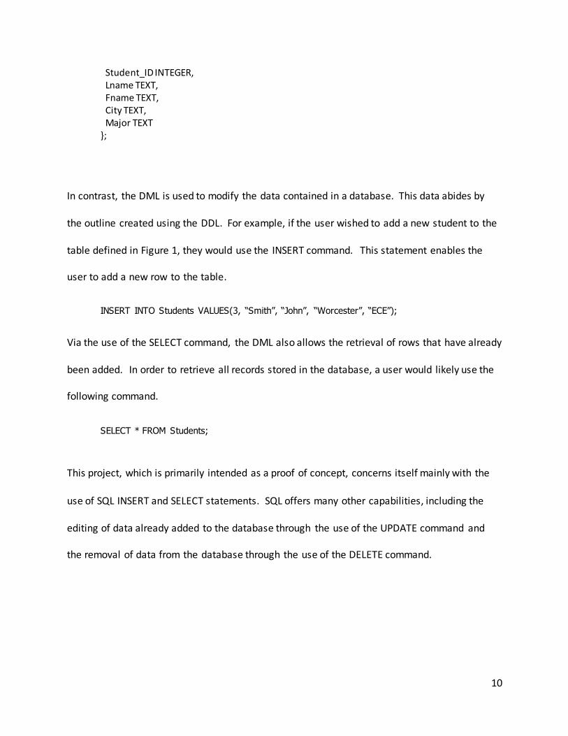
Student_ID INTEGER, Lname TEXT, Fname TEXT, City TEXT, Major TEXT };
In contrast, the DML is used to modify the data contained in a database. This data abides by
the outline created using the DDL. For example, if the user wished to add a new student to the
table defined in Figure 1, they would use the INSERT command. This statement enables the
user to add a new row to the table.
INSERT INTO Students VALUES(3, “Smith”, “John”, “Worcester”, “ECE”);
Via the use of the SELECT command, the DML also allows the retrieval of rows that have already
been added. In order to retrieve all records stored in the database, a user would likely use the
following command.
SELECT * FROM Students;
This project, which is primarily intended as a proof of concept, concerns itself mainly with the
use of SQL INSERT and SELECT statements. SQL offers many other capabilities, including the
editing of data already added to the database through the use of the UPDATE command and
the removal of data from the database through the use of the DELETE command.

11
4.2.3 Overview of Relational Database Management Systems
There is an assortment of Relational Database Management Systems (DBMS) that implement
SQL commands and Codd’s relational model. Some of the most prevalent systems include
Oracle, Microsoft SQL Server, PostgreSQL, and SQLite [8].
Oracle and Microsoft SQL Server Databases are proprietary enterprise-grade database
solutions. They are intended to handle vast amounts of data stored centrally on a database
server [9] [10]. PostgreSQL is an open-source DBMS; it boasts enterprise-grade power and
exceptional SQL standards compliance [11].
4.2.4 SQLite
The implementation chosen for this project is SQLite, version 3.7.6.3. SQLite is an open source
DBMS that is fundamentally different from the implementations discussed above. Instead of
following a client-server model, it is meant to “provide local data storage for individual
applications and devices” [12]. It claims to compete not with the larger scale server-client
database systems discussed previously, but with the fopen() system call. It is used in many
areas, including embedded systems, small websites, and data analysis. However, SQLite is not
well suited for most networking applications, high concurrency, or data sets larger than a
terabyte. Given these simplifications, SQLite is much more lightweight than other DBMSs
available. This fact makes it more straightforward for a developer to understand and make
changes to the system.
4.3 Classification of Machine Architectures
In 1966, Michael J. Flynn proposed a classification for computer architectures. The system
describes the number of concurrent operations and the amount of data the instructions

12
operate on. The classification is broken into four classes: Single Instruction – Single Data (SISD),
Single Instruction – Multiple Data (SIMD), Multiple Instruction – Single Data (MISD), and
Multiple Instruction, Multiple Data (MIMD) [13]. This project will focus on two of these
architectures, namely SISD and SIMD.
4.3.1 Single Instruction – Single Data
The simplest of Flynn’s classifications, SISD, is implemented as a single core processor. In this
architecture, single machine instructions are run sequentially on single pieces of data in
memory. Figure 3 demonstrates this behavior; each arrow signifies a single instruction, and
each instruction is executed at a different point on the arbitrary time scale.
Figure 3. Single Instruction, Single Data
4.3.2 Single Instruction – Multiple Data
In contrast to the traditional CPU SISD architecture the SIMD architecture executes a single
instruction on multiple memory locations in parallel (SIMD). Figure 4 demonstrates this
behavior; it shows the data at each location in memory being operated on simultaneously.

13
Figure 4. Single Instruction, Multiple Data
This design is implemented by a piece of hardware called the Graphics Processing Unit, or GPU.
4.4 GPU
4.4.1 History of the GPU
GPUs, known colloquially as video cards, emerged out of necessity in the early 1990s to
accelerate the 2d graphics in GUI systems like Microsoft Windows. At a similar time, a
company called Silicon Graphics released a programming interface called OpenGL to its graphics
hardware. They did this for two ends: to popularize 3d graphics, and to secure OpenGL a place
as the industry standard in graphics programming [14].
In 2001, NVIDIA released their GeForce 3 series chip, which implemented Microsoft’s DirectX
8.0. This meant their hardware contained programmable vertex and pixel shaders, which
allowed developers some precise control over the actual operations being performed on the
GPU [14].

14
4.4.2 Graphics Operations on GPUs
GPUs can now be used to speed up graphics as well as non-graphics tasks. Graphics operations
are achieved by processing data through a pipeline of smaller, parallelizable tasks. Figure 5
demonstrates the DirectX pipeline as an example of a graphics pipeline.
Figure 5. DirectX Graphics Pipeline [15]
A simplified diagram of the OpenGL graphics pipeline is shown in Figure 5, and is at a level of
depth adequate for this explanation [16]. Each stage of the graphics pipeline is very similar in
concept, so the Vertex Processing stage is chosen for further analysis. The primary purpose of
the Vertex Processing stage is to transform the information in a vertex data structure to a
location on-screen [17]. This is accomplished through the use of a program called the vertex
shader. One instance of the vertex shader is run on the GPU for each vertex element to be
displayed [18]. Ideally, every vertex would be operated on in parallel, but this is limited in
practice by the number of cores available on the GPU.
4.4.3 General Purpose GPU Programming
These shaders expect to receive graphics data (e.g. color, location) as arguments, and expect to
return modified graphical data as outputs. However, within the shader, these values are simply
arbitrary numeric values on which the programmer can perform arbitrary operations.

15
Developers soon began to write code in the shaders for more generic number-crunching tasks,
by transferring arbitrary information posing as graphical information back and forth between
the CPU and GPU. This was the birth of General Purpose GPU (GPGPU) Programming [14].
4.4.4 CPU vs. GPU
The modern CPU typically has a higher clock rate than the GPU. While the current generation
Intel and AMD processors typically have clock rates on the order of 3-4GHz [19] [20], current
NVIDIA cards like the GeForce GTX 980 falls just over 1GHz [21]. However, while a CPU will
likely have 2-4 processing cores, a GPU may have as many as 1-2 thousand [21]. Each of these
cores is lower power than a CPU core, and thus is suited to less complex operations. GPUs work
well in environments where many small tasks can be performed in parallel to achieve some
larger goal.
4.4.5 GPGPU Applications
Many numerical algorithms can be made faster through GPGPU programming. Successful
acceleration has been achieved in the areas of crypto-currency mining, scientific computing,
image processing, and many others [22].
GPUs have been successfully used to speed up many diverse applications. For instance, there
exists a program called cRARk, whose purpose is to crack forgotten passwords on Windows RAR
archives. Developed by a man named Pavel Semjanov, this program runs on any modern
NVIDIA GPU [23]. CRARk boasts a speedup from 283 password checks per second on traditional
CPU-based methods to 4281 per second on GPUs [24].

16
NVIDIA lists a wide variety of GPGPU applications on their website [25]. Some of the more
interesting uses include: acceleration for MATLAB (up to 22 times speedup) [26], a molecular
dynamics simulator called LAMMPS (up to 18 times speedup) [27], and a life sciences 3D
visualizer called Amira (up to 70 times speedup) [28].
4.4.6 GPGPU Restrictions
Perhaps the largest restriction on the processing of a GPU is data transfer rate between the
CPU and GPU [29]. In order for the GPU to process data, the CPU must transfer data from its
memory across the computer’s bus to GPU memory. This is a slow process, and must be
repeated in the opposite direction once the GPU has finished its work. Figure 6 illustrates these
transfers.
Figure 6. Data Transfer between CPU & GPU
Consequently, the use of the GPU is best suited in situations where many operations can be
performed on data, with relatively few data transfers. Otherwise, the relative processing speed
on the GPU may become irrelevant due to the transfer overhead.
4.5 CUDA
In 2006, NVIDIA Corporation released CUDA (Compute Unified Device Architecture) as a
platform for general purpose parallel computing using their GPUs. CUDA allows the
17
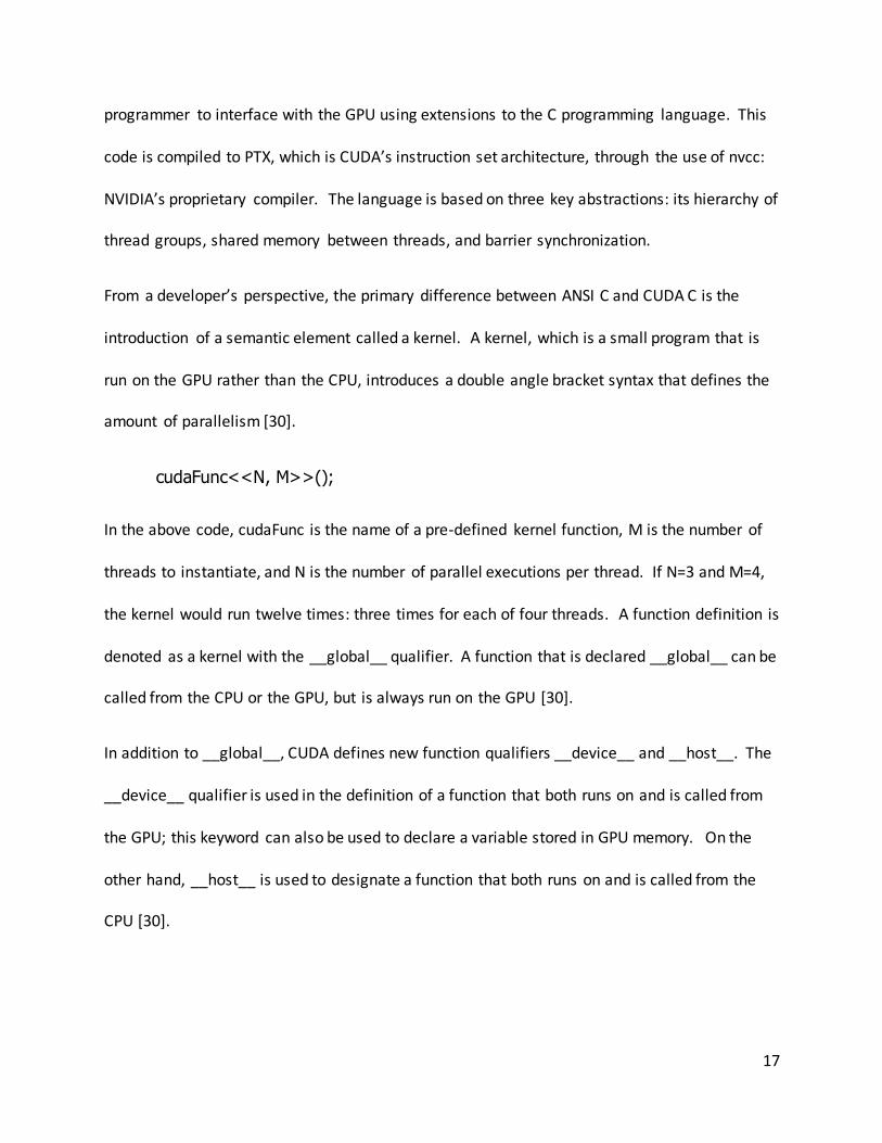
programmer to interface with the GPU using extensions to the C programming language. This
code is compiled to PTX, which is CUDA’s instruction set architecture, through the use of nvcc:
NVIDIA’s proprietary compiler. The language is based on three key abstractions: its hierarchy of
thread groups, shared memory between threads, and barrier synchronization.
From a developer’s perspective, the primary difference between ANSI C and CUDA C is the
introduction of a semantic element called a kernel. A kernel, which is a small program that is
run on the GPU rather than the CPU, introduces a double angle bracket syntax that defines the
amount of parallelism [30].
cudaFunc<<N, M>>();
In the above code, cudaFunc is the name of a pre-defined kernel function, M is the number of
threads to instantiate, and N is the number of parallel executions per thread. If N=3 and M=4,
the kernel would run twelve times: three times for each of four threads. A function definition is
denoted as a kernel with the __global__ qualifier. A function that is declared __global__ can be
called from the CPU or the GPU, but is always run on the GPU [30].
In addition to __global__, CUDA defines new function qualifiers __device__ and __host__. The
__device__ qualifier is used in the definition of a function that both runs on and is called from
the GPU; this keyword can also be used to declare a variable stored in GPU memory. On the
other hand, __host__ is used to designate a function that both runs on and is called from the
CPU [30].

18
5 METHODOLOGY Figure 7 gives an overview of the procedures taken in order to achieve a working virtual table.
Figure 7: Methodology Overview
5.1 Research
The first phase of the project consisted of researching CUDA, SQLite, and GPGPU in general. The
sections below outline the steps taken to gain an understanding of the technologies prevalent
to this MQP.
5.1.1 Tools & libraries
As a first step into the world of CUDA, the first major accomplishment was researching many of
the tools and libraries available. These components were organized in a spreadsheet, and split
into three key sections: infrastructure, libraries, and tools. The three categories are listed in
ascending order of abstraction: infrastructure APIs are low-level building blocks, and libraries
are higher-level collections of infrastructure components. The tools category is an assortment
of programs used to improve the CUDA programming experience (e.g. IDEs and profilers). The
complete spreadsheet is available in Appendix B, but a small snippet is shown below.
CUDA Libraries Research
Linear Algebra Tests
Virtual Table Research
Virtual Table Implementation

19
General Libraries
Name Description URL
AmgX acceleration in the computationally intense linear solver portion of simulations
https://developer.nvidia.com/amgx
ArrayFire GPU function library, including functions for math, signal and image processing, statistics
https://developer.nvidia.com/arrayfire
cuBLAS GPU-accelerated version of the complete standard BLAS library
https://developer.nvidia.com/cublas
cuBLAS-XT set of routines which accelerate Level 3 BLAS (Basic Linear Algebra Subroutine)
https://developer.nvidia.com/cublasxt
CUDA Math Library
collection of standard mathematical functions, providing high performance on NVIDIA GPUs
https://developer.nvidia.com/cuda-math-library
CULA Tools dramatically improve the computation speed of sophisticated mathematics
https://developer.nvidia.com/em-photonics-cula-tools
Figure 8: CUDA Spreadsheet Snippet
The following sections contain tools, libraries, and resources directly of interest to this project.
5.1.1.1 cuBLAS
cuBLAS, or the CUDA Basic Linear Algebra Subroutines (cuBLAS) library, is a GPU-optimized set
of Linear Algebra functions. Just as Thrust is a CUDA analogue to the C++ STL, cuBLAS is based
on Intel’s MKL BLAS. cuBLAS boasts support for all standard BLAS routines, as well as
tremendous speedup. cuBLAS was used in the tests to perform matrix multiplication,
specifically using the cublasSgemm() function. This is useful because this function performs the
matrix multiplications and allows us to transpose the matrices all in one function call.
5.1.1.2 Thrust
One of the most prevalent API sets available is Thrust. Thrust is a library that closely emulates
the C++ Standard Template Library. One useful element of Thrust is the provision of data
structures, such as vectors, that can be created in CPU or GPU-space. The Thrust library was
specifically used in the GPU integer SAXPY algorithm in order to create and populate vectors on
the CPU and GPU, and performing vector transformations.
20
5.1.1.3 Nsight
Nsight is a CUDA development platform released by NVIDIA, with editions for Visual Studio and
Eclipse. This is a useful tool, containing features like GPU-oriented debugging functionality and
code profiling. Because much of this development was performed on a virtual machine, Nsight
was not directly used in this project.
5.1.2 CUDA by Example
CUDA by Example [31] is a book written by senior developers of the CUDA platform team. It
contains lessons and examples aimed to get readers working with CUDA as quickly as possible.
In order to gain as much knowledge in this area as possible, a schedule of chapters to read was
designed in order to complete the book in its entirety by the end of the MQP.
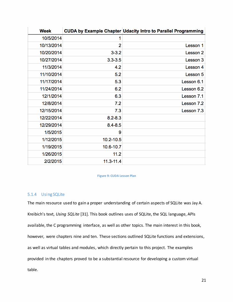
5.1.3 Udacity Intro to Parallel Programming
Udacity offers an introductory-level course on Parallel Programming. Although this course does
not dive as deeply into the language as CUDA by Example, it is a useful resource that should
provide much insight prior to the start of coding. A lesson plan from this course was arranged
to supplement the readings from CUDA by Example, as shown in Figure 9.
21
Figure 9: CUDA Lesson Plan
5.1.4 Using SQLite
The main resource used to gain a proper understanding of certain aspects of SQLite was Jay A.
Kreibich's text, Using SQLite [31]. This book outlines uses of SQLite, the SQL language, APIs
available, the C programming interface, as well as other topics. The main interest in this book,
however, were chapters nine and ten. These sections outlined SQLite functions and extensions,
as well as virtual tables and modules, which directly pertain to this project. The examples
provided in the chapters proved to be a substantial resource for developing a custom virtual
table.

22
5.2 Environment
The following sections describe the environment uses to complete this project.
5.2.1 VirtualBox and Debian
Because of the complexity of installing CUDA on a Windows machine, VirtualBox and a Linux
distribution were required. Debian 7 was the Linux version chosen.
5.2.2 SSH
The local machines used did not have a GPU, so an external resource to run the CUDA code was
necessary. The remote machine all of the code ran on was a SUSE Linux machine. SSH was used
to gain terminal access to modify and run code.
5.2.3 GPU Information
The CUDA installation provides a useful program called deviceQuery that provides all of the
necessary information about the GPU installed in the machine. Figure 10 shows the output of
program for the GPU used in this project.

23
Figure 10: Information of GPU used in this Project
5.3 Linear Algebra Tests
A first area of investigation was to find the types of problems most likely to yield the most
performance improvements, specifically linear algebra operations. These types of problems
directly apply to different users in EMC, specifically the FAST(Fully Automated Storage Tiering)
Engine and the meta-data paging developers. The FAST team runs algorithms that determine
which back-end devices data lives on, ranging from solid-state drives, Serial Attached SCSI (SAS)
drives, and Serial ATA (SATA) drives. The meta-data paging team develops algorithms to ensure
the meta-data associated with active drives are already in memory, using a variety of database
algorithms to keep track of this data.

24
5.3.1 Dot Products
The first test performed was the integer dot product algorithm. The dot product is calculated
with the formula below, given two vectors X and Y with a size of N:
𝑋 ∙ 𝑌 = 𝑋1 ∗ 𝑌1 + 𝑋2 ∗ 𝑌2 +. . . +𝑋𝑁 ∗ 𝑌𝑁
This test was completed by starting with a size of N=100, and incrementing by 1000 until N <
100100. The dot product is one type of linear algebra operation that could be useful to some of
the meta-data paging developers at EMC, who run algorithms to determine if meta-data is
already in memory.
5.3.2 Matrix Multiply
The second test executed to become accustomed to programming in CUDA was the matrix
multiplication algorithm. This test uses the CUBLAS, a commonly used Linear Algebra
Subroutine library, for matrix functions, providing an easy interface to run operations on
matrices with C code. A major issue was the column ordering of the matrices. The CUBLAS
library uses column ordering, while C matrices are stored in row order. Hence, a function was
needed to transpose the matrices when the matrices are transferred onto the GPU, and
transpose the data again once it is transferred onto the host. Square matrices were used in this
example (NxN).
5.3.3 SAXPY
SAXPY (Single-Precision A·X Plus Y) is a combination of scalar multiplication and vector addition.
The chart below shows the timing for running { (a* X) + Y } using on both the CPU and GPU
using the thrust library functions. Thrust here is used to generate the CPU and GPU vectors, and
performs the transformation operations for the GPU. In this graph, the y-axis is a log scale in
25
milliseconds. The vectors the vector size on the x-axis ranges from 100 to 100100 in increments
of 1000. Below is the function used to calculate SAXPY on the CPU.
void saxpy_cpu_float(float A, thrust::host_vector<float>& X, thrust::host_vector<float>& Y)
{
for(int i = 0; i < X.size(); i++)
{
Y[i] = (A * X[i]) + Y[i];
}
}
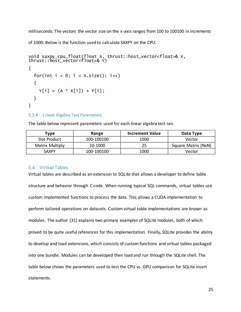
5.3.4 Linear Algebra Test Parameters
The table below represent parameters used for each linear algebra test ran.
Type Range Increment Value Data Type
Dot Product 100-100100 1000 Vector
Matrix Multiply 10-1000 25 Square Matrix (NxN)
SAXPY 100-100100 1000 Vector
5.4 Virtual Tables
Virtual tables are described as an extension to SQLite that allows a developer to define table
structure and behavior through C code. When running typical SQL commands, virtual tables use
custom implemented functions to process the data. This allows a CUDA implementation to
perform tailored operations on datasets. Custom virtual table implementations are known as
modules. The author [31] explains two primary examples of SQLite modules, both of which
proved to be quite useful references for this implementation. Finally, SQLite provides the ability
to develop and load extensions, which consists of custom functions and virtual tables packaged
into one bundle. Modules can be developed then load and run through the SQLite shell. The
table below shows the parameters used to test the CPU vs. GPU comparison for SQLite insert
statements.

26
Table 1: Parameters for SQLite Insertion Benchnmark
Elements CPU GPU Ratio (GPU/CPU)
10 54.546 46.655 0.855333
50 55.836 51.607 0.92426
100 63.451 55.617 0.876535
500 76.378 76.987 1.007974
1000 80.424 111.846 1.390704
5000 190.073 362.673 1.908072
10000 377.843 618.979 1.638191
50000 1621.624 3319.754 2.047179
100000 2716.473 6451.976 2.37513
500000 13766.28 29348.19 2.13189
1000000 30754.51 60059.45 1.952867

27
6 RESULTS
6.1 Linear Algebra Results
The following sections show the performance increases found from CPU to GPU for linear
algebra operations. These performance increases shown below are important for the FAST(Fully
Automated Storage Tiering) Engine and the meta-data paging teams.
6.1.1 Dot Products
As Figure 11 shows, GPUs perform at a relatively consistent level, while the CPU increases
logarithmically as the number of elements in the vector increases. Even as the vector size
increases, the GPU performs at a steady pace. Vector size represents the number of elements in
each of the two vectors input into the dot product algorithm. The crossover point in which the
GPU outperforms the CPU occurs at a vector size of around 200 elements.
Figure 11: Dot Product Algorithm
vector size ≈ 200
28
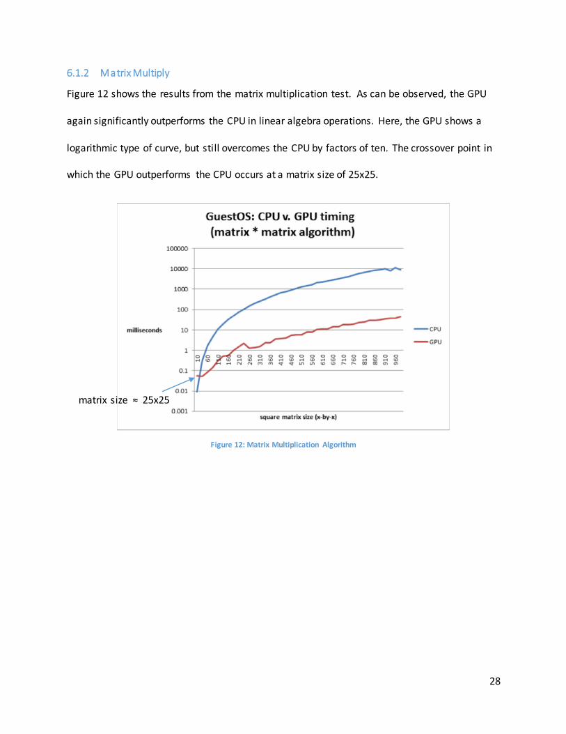
6.1.2 Matrix Multiply
Figure 12 shows the results from the matrix multiplication test. As can be observed, the GPU
again significantly outperforms the CPU in linear algebra operations. Here, the GPU shows a
logarithmic type of curve, but still overcomes the CPU by factors of ten. The crossover point in
which the GPU outperforms the CPU occurs at a matrix size of 25x25.
Figure 12: Matrix Multiplication Algorithm
matrix size ≈ 25x25
29
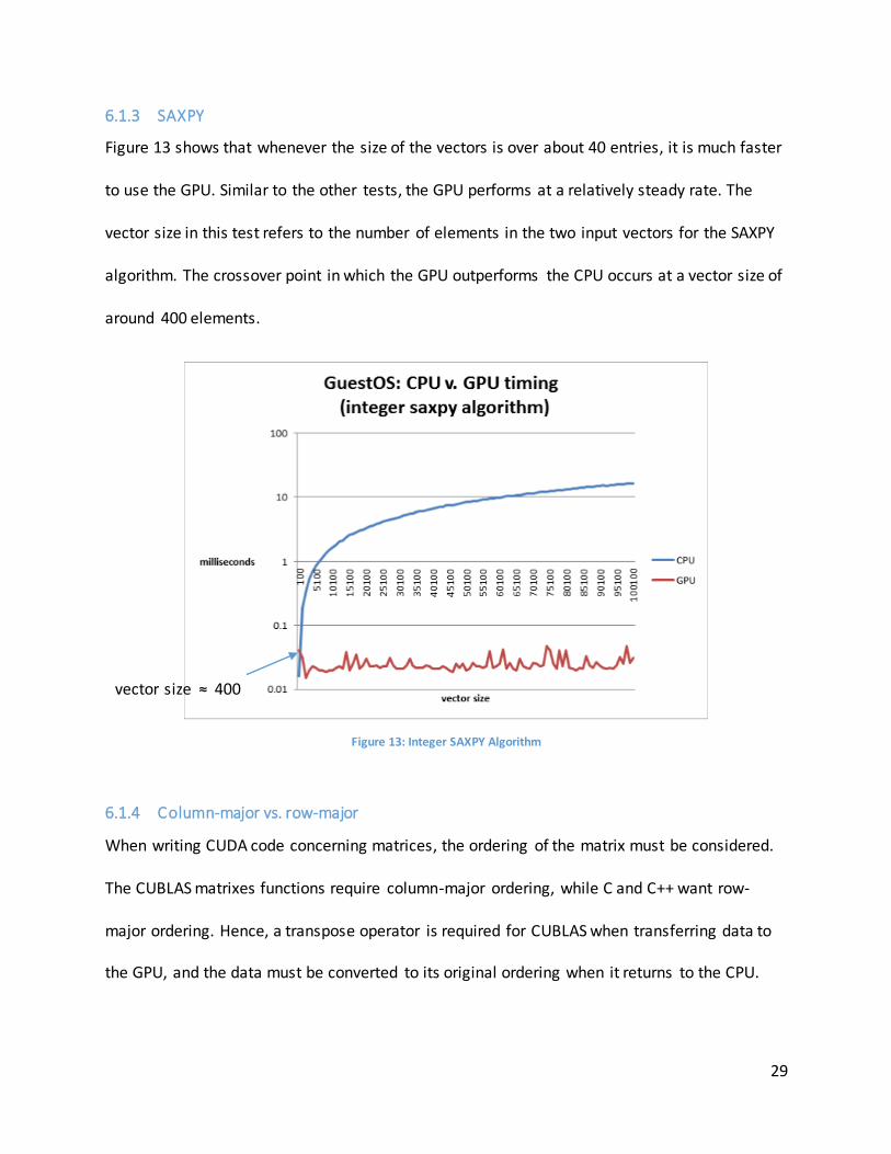
6.1.3 SAXPY
Figure 13 shows that whenever the size of the vectors is over about 40 entries, it is much faster
to use the GPU. Similar to the other tests, the GPU performs at a relatively steady rate. The
vector size in this test refers to the number of elements in the two input vectors for the SAXPY
algorithm. The crossover point in which the GPU outperforms the CPU occurs at a vector size of
around 400 elements.
Figure 13: Integer SAXPY Algorithm
6.1.4 Column-major vs. row-major
When writing CUDA code concerning matrices, the ordering of the matrix must be considered.
The CUBLAS matrixes functions require column-major ordering, while C and C++ want row-
major ordering. Hence, a transpose operator is required for CUBLAS when transferring data to
the GPU, and the data must be converted to its original ordering when it returns to the CPU.
vector size ≈ 400

30
Concerning the virtual table ordering, column major tables will speed up operations such as
"like" and "match," since whole chunks of column data can be examined in parallel. This will
also avoid the need to transpose the database storage from CPU memory to GPU memory,
since the data will be put directly into the GPU.
6.2 Implementing the Virtual Table
The next major step in the project was the implementation of a virtual table with GPU
functionality. The following sections outline the steps taken to complete that goal.
6.2.1 Stripping down book example
Virtual tables are fairly complex, and inherently difficult to debug. Each virtual table extension
must implement a subset of virtual table functions (e.g. xCreate, xConnect, xDisconnect, etc.)
depending on its purpose. To start, SQL functions needed to be mapped to CUDA, determining
a minimal, working set of required virtual table functions. This was accomplished by starting
with the virtual table example, "dblist.c," from Chapter 10 of Using SQLite. The dblist module
provided from the book takes the “PRAGMA database_list” SQLite command output and
presents it as a table. The purpose of this module is to show the necessary functions needed for
a SQLite module.
The next step, for testing purposes, was a function call to the matrix tests described above.
This allowed for CUDA code to be called within SQLite, as shown below.
sqlite3> select doMatrixTest() from sql_database_list where name=”main”;
In order to determine which virtual table functions were necessary, print statements were
added within each function to show when it was being called. In order to create a barebones
31
module, extraneous function implementations were removed and code simplifications were
made. In the end, the functions that needed to be implemented were xConnect, xOpen, xFilter,
xNext, xEof, and xColumn. The following section shows a step-by-step example of how these
functions are used.
The xConnect() function is used to create a virtual table, and is called in response to the
“CREATE VIRTUAL TABLE” statement. This function also establishes a connection to the newly
created virtual table. The xOpen() function is used to create a new cursor for reading or writing
to the virtual table. The xFilter() function is used to search the virtual table. This function takes
in the cursor opened by xOpen(), as well as a search index chosen by the xBestIndex() function.
The xFilter() and xBestIndex() functions are the primary areas in which query optimization
occurs. xNext() is used by the xFilter() function and advances the virtual table cursor the next
row. xColumn() is called multiple times per row, as it extracts the value of the N-th column for
the current row. Finally, the xEof() function determines if the cursor points to a valid row of
data. Hence, this function is called after every xFilter() and xNext() call.
The custom virtual implementation used in this project uses these functions described above,
and removed non-essential functions. This allowed for the above functions to be implemented
with CUDA code.
6.2.2 Memory management
One concern with virtual table performance is memory management. Because column-based
ordering is required for the GPU implementation, memory management becomes considerably
more complicated than row-based models. Hence, the memory management overhead cannot

32
be greater than the performance gains from the column-based pattern matching. To achieve
this, each column must be contiguous in memory. This becomes difficult, as it is uncertain how
many rows may be added, which may lead to a large number of memory reallocations.
For the CPU implementation, memory is allocated based on a fixed amount defined in a
constant. This approach is inefficient, but makes it easier to manage than having varying table
sizes. The GPU table is designed to be relatively more efficient, since it uses a column-major
ordering. This ordering allows for more efficient memory access for parallel searching and
pattern matching, achieving performance gains over normal C row-major ordering. The GPU still
uses a pre-allocated limit to the number of rows that the table can use. This technique is
necessary in order to maintain contiguous memory and limits reallocation. If this strategy was
not used, continuous memory allocations would cause fragmentation in the memory space
available and non-contiguous memory would result in a significant performance hit for parallel
searching. The major penalty on the GPU side occurs when string data is transferred from the
CPU to the GPU and back. Because of this performance loss, it may be an improvement to
perform the searches on the CPU.
6.3 Virtual Table Results
In order to test the effectiveness of a CUDA SQLite virtual table, a set of benchmarks were run
in order to see the GPU comparison. As Figure 14 shows, the CPU significantly outperforms the
GPU as the number of rows increase. This may be due to the memory transfer across the PCI
barrier. A more optimized memory model would greatly increase the effectiveness of this
study, but this implementation did not focus on code optimization as much as developing a
working virtual table.

33
Figure 14: GPU/CPU Insertions Benchmark
Figure 15 shows a zoomed-in version of Figure 14, giving a clearer view of the compressed
range of data points from 10-10000 rows.
Figure 15: GPU/CPU Insertions Benchmark (zoomed)
0
10000
20000
30000
40000
50000
60000
70000
1 10 100 1000 10000 100000 1000000
Tim
e (
ms)
Number of Rows
GPU/CPU Insertions Benchmark
CPU
GPU
0
100
200
300
400
500
600
700
1 10 100 1000 10000
Tim
e (
ms)
Number of Rows
GPU/CPU Insertions Benchmark (zoomed)
CPU
GPU

34
7 CONCLUSIONS
7.1 Viability of leveraging the GPU
Based on the linear algebra tests and the SQLite virtual table implementation, this proof of
concept project could be useful in multiple areas in EMC. As stated above, the FAST Engine and
the meta-data paging developers could benefit from the linear algebra and other types of
problems. Using certain libraries, such as the Thrust or CUBLAS libraries could also be
advantageous for some of their applications. The SQLite virtual table could also be of use for
the meta-data paging team, as well as future work involving a complete port of SQLite to CUDA.
This step would be time consuming, but beneficial for those users.
7.2 OpenCL
OpenCL is an open-source alternative to CUDA. It was developed by KHRONOS Group, well
known as the developers of OpenGL. It will be wise for the successors in this project to
consider migrating the existing codebase from CUDA to OpenCL. This provides a few key
advantages; first and foremost is its multi-vendor support. Though CUDA claims more frequent
updates than OpenCL, its use implies that only NVIDIA GPUs can be used. On the other hand,
OpenCL boasts an ability to run code on any modern GPU [32].

35
8 BIBLIOGRAPHY
[1] "Milestones: 1979-1989," EMC, 2015. [Online]. Available:
http://www.emc.com/corporate/emc-at-glance/milestones/milestones-1989-1979.htm.
[Accessed 1 March 2015].
[2] "EMC: Summary for EMC Corporation Common Stock," Yahoo Finance, 1 March 2015.
[Online]. Available: http://finance.yahoo.com/q?s=EMC. [Accessed 1 March 2015].
[3] "EMC Competitors," Yahoo Finance, 1 March 2015. [Online]. Available: http://finance.yahoo.com/q/co?s=EMC+Competitors. [Accessed 1 March 2015].
[4] E. F. Codd, "Relational completeness of data base sublanguages," Prentice-Hall, 1972.
[5] S. S. L. Edd Dumbill, "An Incredibly Brief Introduction to Relational Databases: Appendix B -
Learning Rails," in Learning Rails, O'Reilly Media, 2008, p. 448.
[6] R. F. B. Donald D. Chamberlin, "SEQUEL: A STRUCTURED ENGLISH QUERY LANGUAGE," IBM
Research Laboratory, San Jose, California, 1974.
[7] "SQL Commands," Art Branch Inc., [Online]. Available: http://www.sqlcommands.net/.
[Accessed 2 March 2015].
[8] "DB-Engines Ranking - popularity ranking of relational DBMS," solid IT, 2015. [Online].
Available: http://db-engines.com/en/ranking/relational+dbms. [Accessed 2 March 2015].
[9] "Database 12c | Oracle," Oracle, 2015. [Online]. Available: https://www.oracle.com/database/index.html. [Accessed 2 March 2015].
[10] "SQL Server 2014 | Microsoft," Microsoft, 2015. [Online]. Available:
http://www.microsoft.com/en-us/server-cloud/products/sql-server/. [Accessed 2 March 2015].
[11] "PostgreSQL: About," The PostgreSQL Global Development Group, 2015. [Online].
Available: http://www.postgresql.org/about/. [Accessed 2 March 2015].
[12] D. R. Hipp, "Appropriate Uses for SQLite," [Online]. Available:
http://sqlite.org/whentouse.html. [Accessed 2 March 2015].
[13] M. J. Flynn, "Some Computer Architectures and Their Effectiveness," IEEE Transactions on
Computers, Vols. c-21, no. 9, pp. 948-960, 1972.
[14] E. K. Jason Sanders, CUDA By Example, Boston: Pearson Education, Inc., 2011.

36
[15] "Direct 3D Architecture," 2015. [Online]. Available: https://i-msdn.sec.s-
msft.com/dynimg/IC412590.png. [Accessed 2 March 2015].
[16] "Rendering Pipeline Overview - OpenGL," 1 January 2015. [Online]. Available: https://www.opengl.org/wiki/Rendering_Pipeline_Overview. [Accessed 2 March 2015].
[17] "Graphics Pipeline Definition from PC Magazine Encyclopedia," PCMag Digital Group, 2015.
[Online]. Available: http://www.pcmag.com/encyclopedia/term/43933/graphics -pipeline.
[Accessed 2 March 2015].
[18] "Vertex Shader - OpenGL.org," 16 January 2015. [Online]. Available: https://www.opengl.org/wiki/Vertex_Shader. [Accessed 2 March 2015].
[19] "5th Generation Intel Core i7 Processors," Intel Corporation, [Online]. Available:
http://www.intel.com/content/www/us/en/processors/core/core-i7-processor.html.
[Accessed 2 March 2015].
[20] "AMD Phenom II Processors," Advanced Micro Devices, Inc, 2015. [Online]. Available:
http://www.amd.com/en-us/products/processors/desktop/phenom-ii. [Accessed 2 March
2015].
[21] "GeForce GTX 980 | Specifications | GeForce," NVIDIA Corporation, 2015. [Online].
Available: http://www.geforce.com/hardware/desktop-gpus/geforce-gtx-
980/specifications. [Accessed 2 March 2015].
[22] "GPGPU.org :: General Purpose computation on Graphics Processing Units," 2015. [Online]. Available: http://gpgpu.org/. [Accessed 3 March 2015].
[23] P. Semjanov, "cRARk - freeware RAR password recovery," 25 July 2014. [Online]. Available:
http://www.crark.net/#purpose. [Accessed 3 March 2015].
[24] N. Mohr, "Do more with graphics: power up with GPGPU," TechRadar, 3 February 2013.
[Online]. Available: http://www.techradar.com/us/news/computing-components/graphics-cards/do-more-with-graphics-power-up-with-gpgpu-1128214. [Accessed 3 March 2015].
[25] "GPU Applications | High Performance Computing," NVIDIA Corporation, 2015. [Online].
Available: http://www.nvidia.com/object/gpu-applications.html. [Accessed 3 March 2015].
[26] "MATLAB Acceleration on Tesla and Quadro GPUs," NVIDIA Corporation, 2015. [Online].
Available: http://www.nvidia.com/object/tesla-matlab-accelerations.html. [Accessed 3
March 2015].
[27] "LAMMPS Molecular Dynamics Simulator," Sandia, 2015. [Online]. Available:

37
http://lammps.sandia.gov/. [Accessed 3 March 2015].
[28] "Amira 3D Software for Life Sciences," FEI, 2015. [Online]. Available:
http://www.fei.com/software/amira-3d-for-life-sciences/. [Accessed 3 March 2015].
[29] M. Harris, "How to Optimize Data Transfers in CUDA C/C++," NVIDA Corporation, 4
December 2012. [Online]. Available: http://devblogs.nvidia.com/parallelforall/how-
optimize-data-transfers-cuda-cc/. [Accessed 3 March 2015].
[30] "Programming Guide :: CUDA Toolkit Documentation," NVIDIA Corporation, 1 August 2014.
[Online]. Available: http://docs.nvidia.com/cuda/cuda-c-programming-guide/#axzz3TLxREdNg. [Accessed 3 March 2015].
[31] J. A. Kreibich, Using SQLite, Sebastopol, CA: O'Reilly, 2010.

38
9 APPENDIX A: TABLE OF TOOLS AND LIBRARIES Infrastructure
Name Description URL
GPUDirect
Enables 3rd party network adapters and other devices to directly read and write CUDA host and device memory on NVIDIA Tesla™ and Quadro™ products. GPUDirect technology also includes direct transfers between GPUs
https://developer.nvidia.com/gpudirect
LLVM
open source compiler infrastructure on which NVIDIA's CUDA Compiler (NVCC) is based on. Developers can create or extend programming languages with support for GPU acceleration using the CUDA Compiler SDK
https://developer.nvidia.com/cuda-llvm-compiler
MPI Solutions for GPUs
enables applications threads to communicate across compute nodes, supports GPU accelerated nodes
https://developer.nvidia.com/mpi-solutions-gpus
OpenACC
collection of compiler directives to specify loops and regions of code in standard C, C++ and Fortran to be offloaded from a host CPU to an attached accelerator
http://www.openacc-standard.org/
Thrust
open source library of parallel algorithms and data structures. Perform GPU accelerated sort, scan, transform, and reductions with just a few lines of code
https://developer.nvidia.com/thrust https://code.google.com/p/thrust/
General Libraries
Name Description URL
AmgX acceleration in the computationally intense linear solver portion of simulations
https://developer.nvidia.com/amgx
ArrayFire GPU function library, including functions for math, signal and image processing, statistics
https://developer.nvidia.com/arrayfire
cuBLAS GPU-accelerated version of the complete standard BLAS library
https://developer.nvidia.com/cublas
cuBLAS-XT set of routines which accelerate Level 3 BLAS (Basic Linear Algebra Subroutine)
https://developer.nvidia.com/cublasxt
CUDA Math Library
collection of standard mathematical functions, providing high performance on NVIDIA GPUs
https://developer.nvidia.com/cuda-math-library
CULA Tools dramatically improve the computation speed of sophisticated mathematics
https://developer.nvidia.com/em-photonics-cula-tools
cuDNN GPU accelerated library of primitives for deep neural networks
https://developer.nvidia.com/cuDNN
cuFFT simple interface for computing FFTs up to 10x faster
https://developer.nvidia.com/cufft
cuRAND library performs high quality GPU accelerated random number generation (RNG)
https://developer.nvidia.com/curand
cuSPARSE collection of basic linear algebra subroutines https://developer.nvidia.com/cu

39
used for sparse matrices sparse
Geometry Performance Primatives(GPP)
geometry engine that is optimized for GPU acceleration
https://developer.nvidia.com/geometric-performance-primitives-gpp
HiPLAR
(High Performance Linear Algebra in R) delivers high performance linear algebra (LA) routines for the R platform for statistical computing
https://developer.nvidia.com/hiplar
IMSL Fortran Numerical Library
set of mathematical and statistical functions that offloads work to GPUs
https://developer.nvidia.com/imsl-fortran-numerical-library
KALDI The CUDA matrix library seamless wrapper of CUDA computation
http://kaldi.sourceforge.net/cudamatrix.html
Labview
LabView enables engineers and scientists to create applications using a powerful high level programming language and advanced tools
http://zone.ni.com/devzone/cda/tut/p/id/11972
MAGMA collection of next gen linear algebra routines https://developer.nvidia.com/magma
Math Premium
takes advantage of the NVIDIA CUDA architecture to dramatically accelerate mathematics on the .NET platform
https://developer.nvidia.com/nmath
Mathematics
Mathematicia by Wolfram is a comprehensive technical computing solution ,enabling complex computational applications to be build
https://developer.nvidia.com/matlab-cuda
Matlab Matlab by Mathworks, has native support for CUDA in the Parallel Computing Toolbox
https://developer.nvidia.com/matlab-cuda
NPP
accelerated library with a very large collection of 1000's of image processing primitives and signal processing primitives
https://developer.nvidia.com/npp
NVBIO
C++ framework for High Throughput Sequence Sequence Analysis for both short and long read alignment
https://developer.nvidia.com/nvbio
OpenCV open source library for computer vision, image processing and machine learning
https://developer.nvidia.com/opencv
Paralution
library for sparse iterative methods with special focus on multi-core and accelerator technology such as GPUs
https://developer.nvidia.com/paralution
Tools
Name Description URL
Allinea DDT
single tool that can debug hybrid MPI, OpenMP and CUDA applications on a single workstation or GPU cluster
https://developer.nvidia.com/allinea-ddt
CUDA-GDB
debugging experience that allows you to debug both the CPU and GPU portions of your application simultaneously
https://developer.nvidia.com/cuda-gdb

40
CUDA-MEMCHECK
Identifies memory access errors in your GPU code and allows you to locate and resolve problems quickly. reports runtime execution errors, identifying situations that could result in an “unspecified launch failure” error while your application is running
https://developer.nvidia.com/CUDA-MEMCHECK
NVIDIA CUDA Profiling Tools Interface (CUPTI)
performance analysis tools with detailed information about GPU usage in a system
https://developer.nvidia.com/cuda-profiling-tools-interface
NVIDIA Nsight Development platform, debugging and profile tools http://www.nvidia.com/nsight
NVIDIA Visual Profiler
performance profiling tool to give feedback to optimize CUDA aplications
https://developer.nvidia.com/nvidia-visual-profiler
PAPI CUDA Component
hardware performance counter measurement technology for the NVIDIA CUDA platform which provides access to the hardware counters inside the GPU. Provides detailed performance counter information regarding the execution of GPU kernels
https://developer.nvidia.com/papi-cuda-component
TAU Performance System
profiling and tracing toolkit for performance analysis of hybrid parallel programs written in CUDA, and pyCUDA., and HMPP
http://www.cs.uoregon.edu/research/tau/home.php
TotalView
GUI-based tool that allows you to debug one or many processes/threads with complete control over program execution
https://developer.nvidia.com/totalview-debugger
VampirTrace
performance monitor which comes with CUDA, and PyCUDA support to give detailed insight into the runtime behavior of accelerators. Enables extensive performance analysis and optimization of hybrid programs.
https://developer.nvidia.com/vampirtrace