General Mission Analysis Tool (GMAT) - User Guidegmat.sourceforge.net/doc/R2011a/help-a4.pdf · 1...
170
General Mission Analysis Tool (GMAT) User Guide
Transcript of General Mission Analysis Tool (GMAT) - User Guidegmat.sourceforge.net/doc/R2011a/help-a4.pdf · 1...

General MissionAnalysis Tool (GMAT)
User Guide

General Mission Analysis Tool (GMAT): User Guide2011a
iii
Table of ContentsIntroduction ................................................................................................................ 1
Introducing GMAT .............................................................................................. 1GMAT Interface Design/Philosophy ..................................................................... 1System Requirements ........................................................................................ 1Installation ......................................................................................................... 1Data and Configuration ....................................................................................... 1
File Structure ............................................................................................. 1Configuring GMAT Data Files ..................................................................... 3Configuring the MATLAB Interfaces ............................................................. 4
Support and Resources ...................................................................................... 5Release Notes ........................................................................................................... 6
New Features .................................................................................................... 6OrbitView ................................................................................................... 6User-Defined Celestial Bodies ..................................................................... 6Ephemeris Output ...................................................................................... 7SPICE Integration for Spacecraft ................................................................. 7Plugins ...................................................................................................... 7GUI/Script Synchronization ......................................................................... 8Estimation [Alpha] ...................................................................................... 8User Documentation ................................................................................... 9
Screenshot ( ) ........................................................................................ 9Improvements .................................................................................................... 9
Automatic MATLAB Detection ..................................................................... 9Dynamics Model Numerics ......................................................................... 9Script Editor [Windows] .............................................................................. 9Regression Testing ................................................................................... 10Visual Improvements ................................................................................ 10
Compatibility Changes ...................................................................................... 11Platform Support ...................................................................................... 11Script Syntax Changes ............................................................................. 11
Fixed Issues .................................................................................................... 12Known Issues .................................................................................................. 12
How To .................................................................................................................... 15Reporting mission parameters ........................................................................... 15Running GMAT Scripts from MATLAB ............................................................... 15
Overview .................................................................................................. 15Procedure ................................................................................................ 15
Creating ephemeris files ................................................................................... 17Creating a Report ............................................................................................. 17
Objective and Overview ............................................................................ 17Creating and Configuring the Resource Tree .............................................. 18
Visualizing a trajectory ...................................................................................... 23Samples and Tutorials .............................................................................................. 24
Propagating a Spacecraft ................................................................................. 24Objective and Overview ............................................................................ 24Configuring Resources ............................................................................. 24Configuring the Mission Tree .................................................................... 28Running the Mission ................................................................................. 30
Designing a Hohmann Transfer ......................................................................... 31Objective and Overview ............................................................................ 31Creating and Configuring the Resource Tree .............................................. 32Creating and Configuring the Mission Tree ................................................ 33Running the Mission ................................................................................. 39
LEO Station Keeping ........................................................................................ 40
General Mission Analy-sis Tool (GMAT)
iv
Objective and Overview ............................................................................ 40Creating and Configuring the Resource Tree .............................................. 41Creating and Configuring the Mission Sequence ........................................ 42Running the Mission ................................................................................. 47
Algebraic Optimization ...................................................................................... 48Objective and Overview ............................................................................ 48Creating and Configuring the Resource Tree .............................................. 48Creating and Configuring the Mission Tree ................................................ 50The resulting view of Resource, Mission, and Output Trees ......................... 52Running the Mission ................................................................................. 52
Mars B-Plane Targeting .................................................................................... 53Objective and Overview ............................................................................ 53Creating and Configuring the Resource Tree .............................................. 54Creating and Configuring the Mission Sequence ........................................ 59The resulting view of Resource, Mission, and Output Trees ......................... 65Running the Mission ................................................................................. 65
Reference Guide ...................................................................................................... 67I. Resources .................................................................................................... 69
Array ........................................................................................................ 70Barycenter ............................................................................................... 71CelestialBodies ......................................................................................... 72CoordinateSystem .................................................................................... 75DifferentialCorrector .................................................................................. 76EphemerisFile .......................................................................................... 79EphemerisPropagator ............................................................................... 80FiniteBurn ................................................................................................ 81Formation ................................................................................................. 83FuelTank .................................................................................................. 84GroundStation .......................................................................................... 86ImpulsiveBurn .......................................................................................... 87LibrationPoint ........................................................................................... 89MATLABFunction ...................................................................................... 90OpenGLPlot ............................................................................................. 91Propagator ............................................................................................... 96ReportFile .............................................................................................. 102SolarSystem ........................................................................................... 105Spacecraft .............................................................................................. 107SQP ....................................................................................................... 112String ..................................................................................................... 115Thruster ................................................................................................. 116Variable ................................................................................................. 121VF13adOptimizer .................................................................................... 122XYPlot ................................................................................................... 123
II. Commands ................................................................................................. 125Achieve .................................................................................................. 126BeginFiniteBurn ...................................................................................... 127BeginMissionSequence ........................................................................... 128CallFunction ........................................................................................... 129Else ....................................................................................................... 131EndFiniteBurn ......................................................................................... 132Equation ................................................................................................. 133For ......................................................................................................... 134If ............................................................................................................ 136Maneuver ............................................................................................... 138Minimize ................................................................................................. 139NonLinearConstraint ............................................................................... 141Optimize ................................................................................................. 143PenUp ................................................................................................... 145

General Mission Analy-sis Tool (GMAT)
v
PenDown ............................................................................................... 146Propagate .............................................................................................. 147Report .................................................................................................... 150Save ...................................................................................................... 151ScriptEvent ............................................................................................. 152Stop ....................................................................................................... 153Target .................................................................................................... 154Toggle ................................................................................................... 156Vary ....................................................................................................... 158While ..................................................................................................... 161
Index ..................................................................................................................... 163

vi
List of Tables1. Multiple platforms ................................................................................................. 122. Windows .............................................................................................................. 133. Mac OS X ............................................................................................................ 144. Linux ................................................................................................................... 14

vii
List of Examples1. Creating an array ................................................................................................. 702. Creating and populating a matrix ........................................................................... 703. Example Script ..................................................................................................... 794. Example Script ..................................................................................................... 805. Example Script ..................................................................................................... 836. Creating a default FuelTank and attaching it to a Spacecraft ................................... 857. Example Script ..................................................................................................... 868. Example Script ..................................................................................................... 909. Creating a default Spacecraft .............................................................................. 11110. Example Script ................................................................................................. 12211. Targeting geosynchronous orbit using an impulsive burn ..................................... 155
1
IntroductionIntroducing GMAT
GMAT is an open-source mission analysis and design tool.
GMAT Interface Design/Philosophy
System Requirements
Installation
Data and ConfigurationBelow we discuss the files and data distributed with GMAT and that are required for GMATexecution. GMAT requires many data files such as planetary ephemeris, Earth orientationdata, leap second files and gravity files to name just a few. Below we describe how thosefiles are organized and describe the controls provided so that you can customize the datafiles GMAT uses at run time.
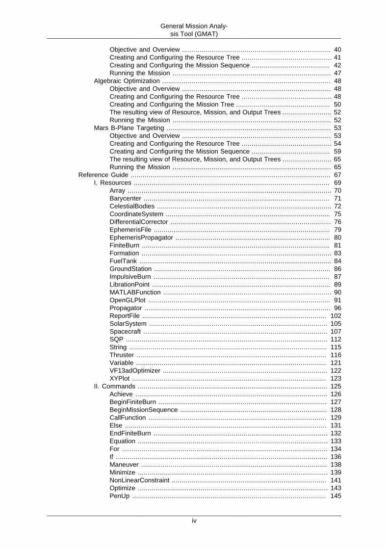
File StructureThe default directory structure for GMAT is shown below and is broken down into eight maindirectories. These directories organize the files and data used to run GMAT including binarylibraries, data files, texture maps, to 3-D models among many others. The only two files inthe GMAT root directory are the license.txt file and the README.txt file. A summary of thecontents of each folder is described in further detail in the sections below.
GMAT Directory Structure
bin Folder
The bin filder contains all binary files required for the core functionality in GMAT (third-par-ty, alpha and beta libraries are placed in the plugins folder). These libraries include the exe-cutable file (GMAT.exe on Windows, GMAT.app on Mac, etc.) and libraries for the GUI. Thebin folder also contains two text files: gmat_startup_file.txt, and gmat.ini. The startup file is
Introduction
2
discussed in detail in a separate section below. The gmat.ini files is used to configure someGUI panels, set paths to external web links, and define "tool tip" messages.
data Folder
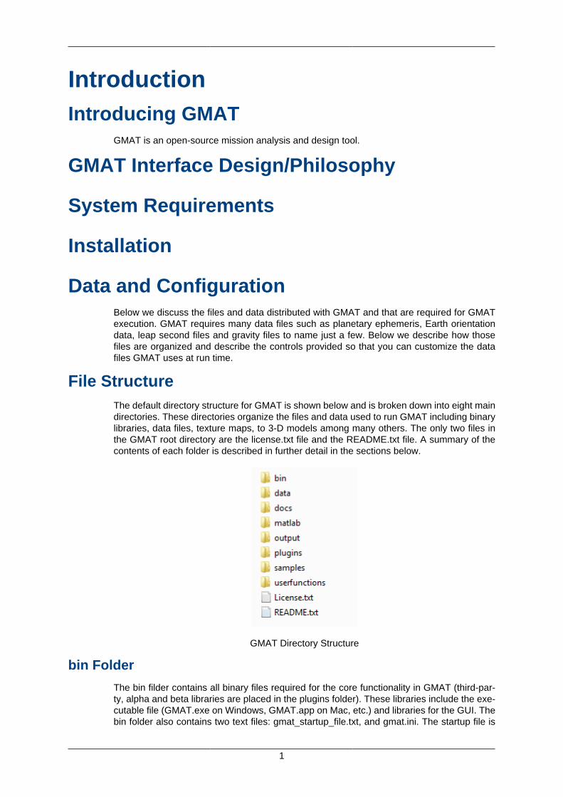
The data folder contains all data files required to run GMAT and is organized accordingto data types as shown in the figure below. The gravity folder contains a folder for eachdefault central body modeled in GMAT and in those folders are files containing gravitationalcoefficients. The gui_config folder contains files for configuring some of the dialog boxes forGMAT Resources and Commands. These files allow you to custom configure a GUI for auser-provided plugin. Furthermore, some of the built-in dialog box designs employ an ini filefor their configuration.
data Folder Structure
The graphics folder contains four subfolders: splash, stars, icons and texture. The splashfolder contains the GMAT splash screen that is displayed briefly while GMAT is initializing.The stars folder contains a star catalogue used for displaying stars in 3D graphics. The texturefolder contains texture maps used for 3D graphics. The icons folder contains graphics filesfor icons and images loaded at run time. These include the GMAT logo, images used onthe about panel and welcome screen, and icons for the Toolbar, Resource Tree and MissionTree.
The planetary_coeff folder contains Earth Orientation Parameters (EOP) provided by the In-ternational Earth Rotation Service (IERS) and nutation coefficients for different nutation the-ories. The planetary_ephem folder contains two folders: de and spk. The de folder containsthe binary Digital Ephemeris DE405 files for the 8 planets, the Moon, and pluto developedand distributed by JPL. The spk folder contains an spk kernel built from the DE421 file andkernels for selected comets, asteroids and moons. All ephemeris files distributed with GMATare in the little-endian representation.
The last two sub-folders in the data folder are time and vehicle. The time folder contains theJPL leap second kernel naif0009.tls and the GMAT leap second file tai-utc.dat. The vehiclefolder contains two sub folders: ephem and models. The ephem subfolder contains SPKephemeris files - including orbit, attitude, frame, and time kernels - for selected spacecraft.The models folder contains 3D model files.
docs Folder
Documentation for GMAT is contained in the docs folder and includes PDF versions of theUser's Guide, Mathematical Specification, Design Specification, and Requirements Specifi-cation to name a few. There is also a subfolder named help that contains html help files.
matlab Folder
The matlab folder contains m-files required for GMAT's MATLAB interfaces including theinterface to fmincon, and interfaces for driving GMAT from MATLAB. All files in the matlabfolder must be included in your MATLAB path for the MATLAB interfaces to function properly.
Introduction
3
output Folder
The output folder is the default location for file output such as ephemeris files and reportfiles. If no path information is provided for reports or ephemeris files created during a GMATsession, then those files will be written to the output folder.
plugins Folder
The plugins folder is for third-party libraries and for functionality that is still in alpha or betastatus. A "proprietary" sub folder within the plugins directory is for third-party libraries thatcannot be distributed as open source files and is an empty folder in the open source distri-bution.
samples Folder
The samples folder contains many sample missions ranging from Hohmann transfer to Li-bration point station-keeping, to Mars B-Plane targetting. These files are intended to demon-strate GMAT's capabilities and to provide you with potential staring points for building com-mon mission types for your application and flight regime.
userfunctions Folder
The userfunctions folder contains two subfolders: gmat and matlab. These folders are wheregmat and matlab functions are stored that are called in the GMAT command sequences forsample missions distributed with GMAT. You can also store your own custom GMAT andMATLAB functions in these folders.
Configuring GMAT Data FilesYou can configure the data files GMAT loads at run time by editing the file namedgmat_startup_file.txt located in the bin directory. The startup file contains path information tofiles such as ephemeris, earth orientation data and graphics files among others. By editingthe startup file, you can customize which files are loaded and used during a GMAT session.Below we describe the customization features available in the startup file. The order of linesin the startup file does not matter.
Leap Second and EOP files
GMAT reads several files that are used for high fidelity modelling of time and coordinatesystems. These files are the leap second files and the Earth Orientation Parameters (EOP)provided by the IERS. The EOP file is updated daily by the IERS. To update your local filewith the latest data, simply replace the data in file eopc04.62-now, (located in the directory ./data/planetary_coeff/ ) with the data provided by the IERS in the link here. There are two leapsecond files provided with GMAT. The file named naif0009.tls located in the .\data\time folderis used by the JPL SPICE libraries when computing ephemeredes. When a new leap seondis added, you can replace your old SPICE leap second file with the new file located here here.
GMAT reads the file tai-utc.dat in the .\data\time folder for all time computations requiring leapseconds that are not performed by the SPICE utilities. You can modify this file if a new leapsecond is added by simply duplicating the last row and updating it with the correct informationfor the new leap second. For example, if a new leapsecond were added on 01 Jul 2013, thenyou would add the following line to the tai-utc.dat file:
2013 JUL 1 =JD 2456474.5 TAI-UTC= 35.0 S + (MJD - 41317.) X 0.0
Loading Custom Plugins
Custom plugins are loaded by adding a line to your startup file describing the name andlocation of the plugin library. In order for a plugin to work with GMAT, the plugin library must
Introduction
4
be placed in the folder referenced in the startup file. You specify the path to a plugin using the"PLUGIN" keyword and specify the file by providing its name without the file extension (.dllon Windows). For example, to load a Windows plugin named libVF13Optimizer.dll located inthe \bin\proprietary folder, you add this line to your startup file:
PLUGIN = ./proprietary/libVF13Optimizer
User-defined Function Paths
If you create custom GMAT or MATLAB functions for your application, you can provide thepath to those files and GMAT will locate them at run time. The default startup file is configuredso you can place GMAT files in the ./userfunctions/gmat folder and place MATLAB functionsin the /userfunctions/matlab folder GMAT automatically searches those locatations at runtime. You can change the location of the search path to your GMAT or MATLAB functionsby changing these lines in your startup file to reflect the location of your files with respectto the GMAT bin folder:
GMAT_FUNCTION_PATH = ../userfunctions/gmat MATLAB_FUNCTION_PATH = ../userfunctions/matlab
If you wish to organize your custom functions in multiple folders, you can add multiple searchpaths to the startup file. For example,
GMAT_FUNCTION_PATH = ../MyFunctions/utils GMAT_FUNCTION_PATH = ../MyFunctions/StateConversion GMAT_FUNCTION_PATH = ../MyFunctions/TimeConversion
Configuring the MATLAB InterfacesGMAT supports several MATLAB interfaces and to use these interfaces the following MAT-LAB folders must be added to your system path:
MATLAB/bin/win32 MATLAB/bin MATLAB/runtime/win32
Caution
The above folders are added to your system path during MATLAB installa-tion. However, for some versions of MATLAB (2010a for example), MATLABand Windows are distributed with libraries that have the same name. This maycause the Windows libraries to load instead of the MATLAB libraries. As a re-sult, you may need to put the folders above at the beginning of your systempath.
If you have multilple versions of MATLAB installed, GMAT will use the version that appearsfirst in your system path and that version must be registered as a COM server using theMATLAB regserver command. To register the desired version of MATLAB, using a commandprompt change directory to the bin folder of the desired MATLAB release and run the followingcommand.
matlab.exe -regserver

Introduction
5
Finally you must add to your MATLAB path all files in the matlab directory which is locatedin the GMAT root directory.
Support and Resources
6
Release NotesThe General Mission Analysis Tool (GMAT) version R2011a was released April 29, 2011 onthe following platforms:
Windows (XP, Vista, 7) Beta
Mac OS X (10.6) Alpha
Linux Alpha
This is the first release since September 2008, and is the 4th public release for the project.In this release:
• 100,000 lines of code were added• 798 bugs were opened and 733 were closed• Code was contributed by 9 developers from 4 organizations• 6216 system tests were written and run nightly
New Features
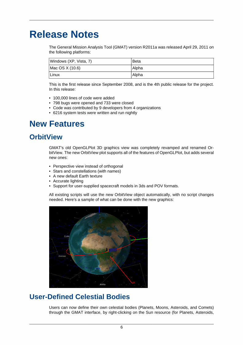
OrbitViewGMAT's old OpenGLPlot 3D graphics view was completely revamped and renamed Or-bitView. The new OrbitView plot supports all of the features of OpenGLPlot, but adds severalnew ones:
• Perspective view instead of orthogonal• Stars and constellations (with names)• A new default Earth texture• Accurate lighting• Support for user-supplied spacecraft models in 3ds and POV formats.
All existing scripts will use the new OrbitView object automatically, with no script changesneeded. Here's a sample of what can be done with the new graphics:
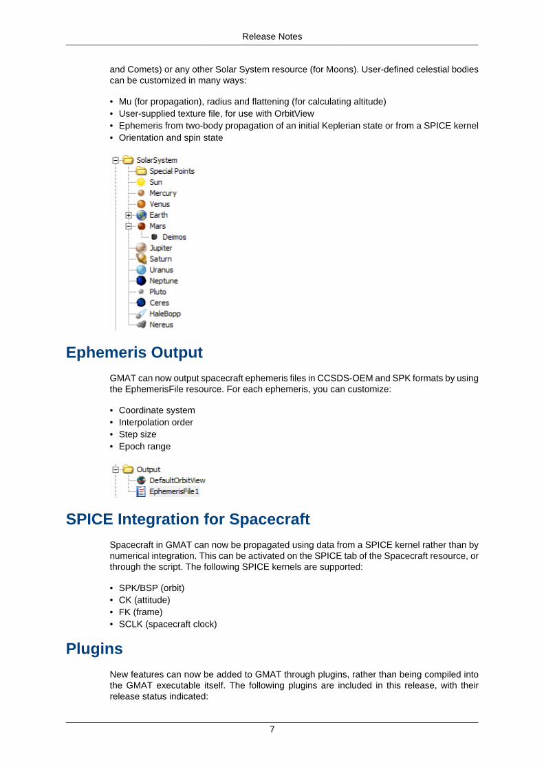
User-Defined Celestial BodiesUsers can now define their own celestial bodies (Planets, Moons, Asteroids, and Comets)through the GMAT interface, by right-clicking on the Sun resource (for Planets, Asteroids,
Release Notes
7
and Comets) or any other Solar System resource (for Moons). User-defined celestial bodiescan be customized in many ways:
• Mu (for propagation), radius and flattening (for calculating altitude)• User-supplied texture file, for use with OrbitView• Ephemeris from two-body propagation of an initial Keplerian state or from a SPICE kernel• Orientation and spin state
Ephemeris OutputGMAT can now output spacecraft ephemeris files in CCSDS-OEM and SPK formats by usingthe EphemerisFile resource. For each ephemeris, you can customize:
• Coordinate system• Interpolation order• Step size• Epoch range
SPICE Integration for SpacecraftSpacecraft in GMAT can now be propagated using data from a SPICE kernel rather than bynumerical integration. This can be activated on the SPICE tab of the Spacecraft resource, orthrough the script. The following SPICE kernels are supported:
• SPK/BSP (orbit)• CK (attitude)• FK (frame)• SCLK (spacecraft clock)
PluginsNew features can now be added to GMAT through plugins, rather than being compiled intothe GMAT executable itself. The following plugins are included in this release, with theirrelease status indicated:
Release Notes
8
libMatlabPlugin Beta
libFminconOptimizer (Windows only) Beta
libGmatEstimation Alpha (preview)
Plugins can be enabled or disabled through the startup file (gmat_startup_file.txt),located in the GMAT bin directory. All plugins are disabled by default.
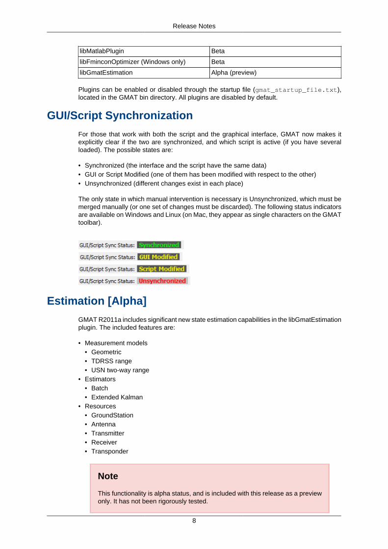
GUI/Script Synchronization
For those that work with both the script and the graphical interface, GMAT now makes itexplicitly clear if the two are synchronized, and which script is active (if you have severalloaded). The possible states are:
• Synchronized (the interface and the script have the same data)• GUI or Script Modified (one of them has been modified with respect to the other)• Unsynchronized (different changes exist in each place)
The only state in which manual intervention is necessary is Unsynchronized, which must bemerged manually (or one set of changes must be discarded). The following status indicatorsare available on Windows and Linux (on Mac, they appear as single characters on the GMATtoolbar).
Estimation [Alpha]
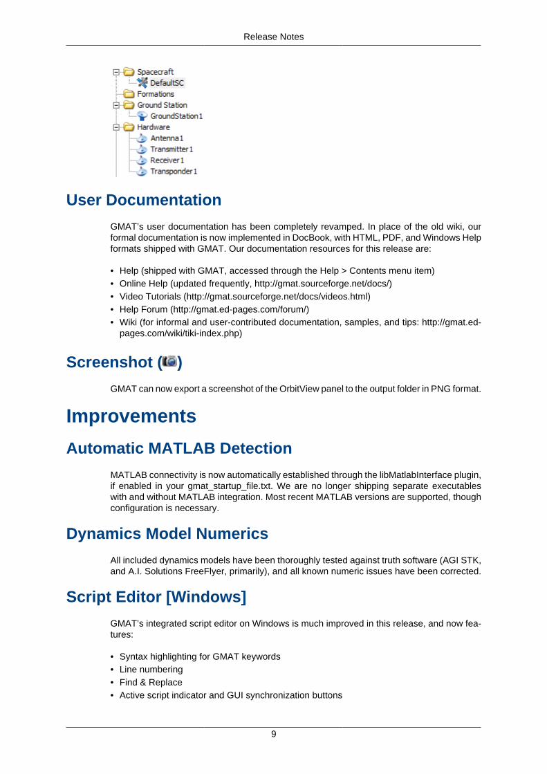
GMAT R2011a includes significant new state estimation capabilities in the libGmatEstimationplugin. The included features are:
• Measurement models• Geometric• TDRSS range• USN two-way range
• Estimators• Batch• Extended Kalman
• Resources• GroundStation• Antenna• Transmitter• Receiver• Transponder
Note
This functionality is alpha status, and is included with this release as a previewonly. It has not been rigorously tested.
Release Notes
9
User Documentation
GMAT’s user documentation has been completely revamped. In place of the old wiki, ourformal documentation is now implemented in DocBook, with HTML, PDF, and Windows Helpformats shipped with GMAT. Our documentation resources for this release are:
• Help (shipped with GMAT, accessed through the Help > Contents menu item)• Online Help (updated frequently, http://gmat.sourceforge.net/docs/)• Video Tutorials (http://gmat.sourceforge.net/docs/videos.html)• Help Forum (http://gmat.ed-pages.com/forum/)• Wiki (for informal and user-contributed documentation, samples, and tips: http://gmat.ed-
pages.com/wiki/tiki-index.php)
Screenshot ( )
GMAT can now export a screenshot of the OrbitView panel to the output folder in PNG format.
Improvements
Automatic MATLAB Detection
MATLAB connectivity is now automatically established through the libMatlabInterface plugin,if enabled in your gmat_startup_file.txt. We are no longer shipping separate executableswith and without MATLAB integration. Most recent MATLAB versions are supported, thoughconfiguration is necessary.
Dynamics Model Numerics
All included dynamics models have been thoroughly tested against truth software (AGI STK,and A.I. Solutions FreeFlyer, primarily), and all known numeric issues have been corrected.
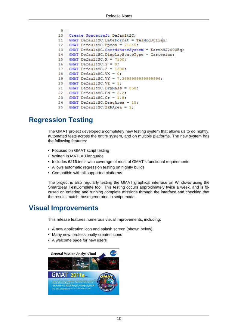
Script Editor [Windows]
GMAT’s integrated script editor on Windows is much improved in this release, and now fea-tures:
• Syntax highlighting for GMAT keywords• Line numbering• Find & Replace• Active script indicator and GUI synchronization buttons
Release Notes
10
Regression Testing
The GMAT project developed a completely new testing system that allows us to do nightly,automated tests across the entire system, and on multiple platforms. The new system hasthe following features:
• Focused on GMAT script testing• Written in MATLAB language• Includes 6216 tests with coverage of most of GMAT’s functional requirements• Allows automatic regression testing on nightly builds• Compatible with all supported platforms
The project is also regularly testing the GMAT graphical interface on Windows using theSmartBear TestComplete tool. This testing occurs approximately twice a week, and is fo-cused on entering and running complete missions through the interface and checking thatthe results match those generated in script mode.
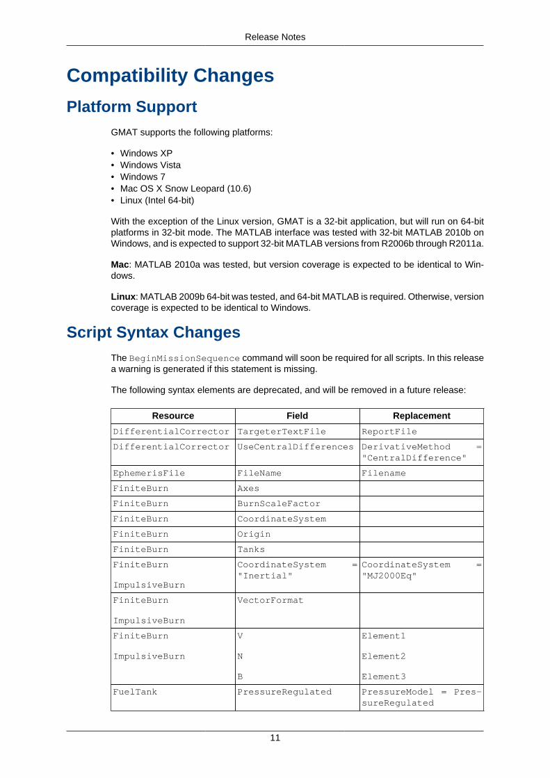
Visual Improvements
This release features numerous visual improvements, including:
• A new application icon and splash screen (shown below)• Many new, professionally-created icons• A welcome page for new users
Release Notes
11
Compatibility Changes
Platform SupportGMAT supports the following platforms:
• Windows XP• Windows Vista• Windows 7• Mac OS X Snow Leopard (10.6)• Linux (Intel 64-bit)
With the exception of the Linux version, GMAT is a 32-bit application, but will run on 64-bitplatforms in 32-bit mode. The MATLAB interface was tested with 32-bit MATLAB 2010b onWindows, and is expected to support 32-bit MATLAB versions from R2006b through R2011a.
Mac: MATLAB 2010a was tested, but version coverage is expected to be identical to Win-dows.
Linux: MATLAB 2009b 64-bit was tested, and 64-bit MATLAB is required. Otherwise, versioncoverage is expected to be identical to Windows.
Script Syntax ChangesThe BeginMissionSequence command will soon be required for all scripts. In this releasea warning is generated if this statement is missing.
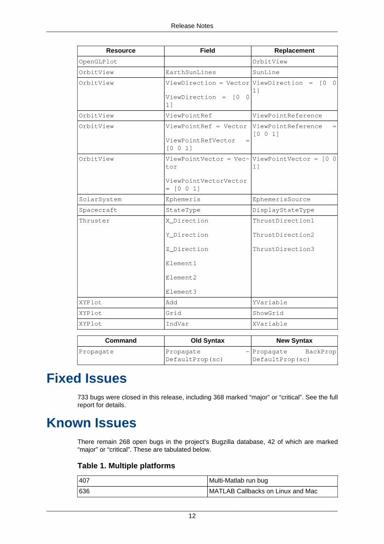
The following syntax elements are deprecated, and will be removed in a future release:
Resource Field Replacement
DifferentialCorrector TargeterTextFile ReportFile
DifferentialCorrector UseCentralDifferences DerivativeMethod ="CentralDifference"
EphemerisFile FileName Filename
FiniteBurn Axes
FiniteBurn BurnScaleFactor
FiniteBurn CoordinateSystem
FiniteBurn Origin
FiniteBurn Tanks
FiniteBurn
ImpulsiveBurn
CoordinateSystem ="Inertial"
CoordinateSystem ="MJ2000Eq"
FiniteBurn
ImpulsiveBurn
VectorFormat
FiniteBurn
ImpulsiveBurn
V
N
B
Element1
Element2
Element3
FuelTank PressureRegulated PressureModel = Pres-sureRegulated
Release Notes
12
Resource Field Replacement
OpenGLPlot OrbitView
OrbitView EarthSunLines SunLine
OrbitView ViewDirection = Vector
ViewDirection = [0 01]
ViewDirection = [0 01]
OrbitView ViewPointRef ViewPointReference
OrbitView ViewPointRef = Vector
ViewPointRefVector =[0 0 1]
ViewPointReference =[0 0 1]
OrbitView ViewPointVector = Vec-tor
ViewPointVectorVector= [0 0 1]
ViewPointVector = [0 01]
SolarSystem Ephemeris EphemerisSource
Spacecraft StateType DisplayStateType
Thruster X_Direction
Y_Direction
Z_Direction
Element1
Element2
Element3
ThrustDirection1
ThrustDirection2
ThrustDirection3
XYPlot Add YVariable
XYPlot Grid ShowGrid
XYPlot IndVar XVariable
Command Old Syntax New Syntax
Propagate Propagate -DefaultProp(sc)
Propagate BackPropDefaultProp(sc)
Fixed Issues733 bugs were closed in this release, including 368 marked “major” or “critical”. See the fullreport for details.
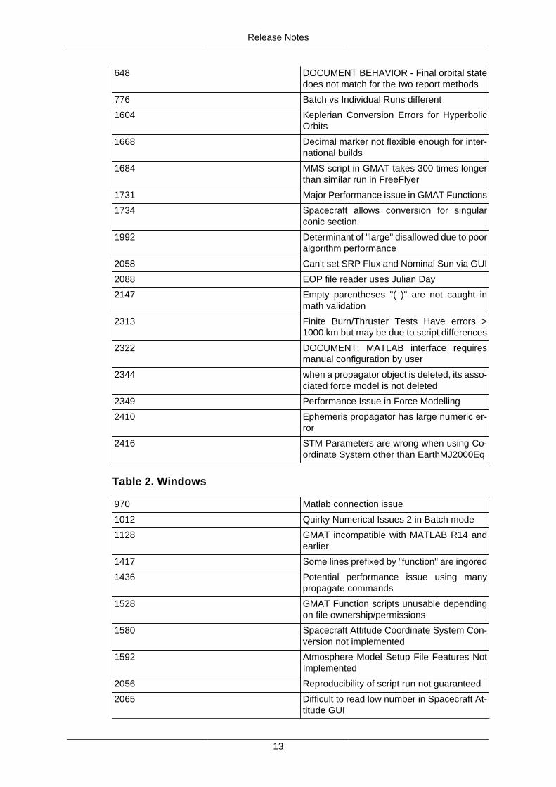
Known IssuesThere remain 268 open bugs in the project’s Bugzilla database, 42 of which are marked“major” or “critical”. These are tabulated below.
Table 1. Multiple platforms
407 Multi-Matlab run bug
636 MATLAB Callbacks on Linux and Mac
Release Notes
13
648 DOCUMENT BEHAVIOR - Final orbital statedoes not match for the two report methods
776 Batch vs Individual Runs different
1604 Keplerian Conversion Errors for HyperbolicOrbits
1668 Decimal marker not flexible enough for inter-national builds
1684 MMS script in GMAT takes 300 times longerthan similar run in FreeFlyer
1731 Major Performance issue in GMAT Functions
1734 Spacecraft allows conversion for singularconic section.
1992 Determinant of "large" disallowed due to pooralgorithm performance
2058 Can't set SRP Flux and Nominal Sun via GUI
2088 EOP file reader uses Julian Day
2147 Empty parentheses "( )" are not caught inmath validation
2313 Finite Burn/Thruster Tests Have errors >1000 km but may be due to script differences
2322 DOCUMENT: MATLAB interface requiresmanual configuration by user
2344 when a propagator object is deleted, its asso-ciated force model is not deleted
2349 Performance Issue in Force Modelling
2410 Ephemeris propagator has large numeric er-ror
2416 STM Parameters are wrong when using Co-ordinate System other than EarthMJ2000Eq
Table 2. Windows
970 Matlab connection issue
1012 Quirky Numerical Issues 2 in Batch mode
1128 GMAT incompatible with MATLAB R14 andearlier
1417 Some lines prefixed by "function" are ingored
1436 Potential performance issue using manypropagate commands
1528 GMAT Function scripts unusable dependingon file ownership/permissions
1580 Spacecraft Attitude Coordinate System Con-version not implemented
1592 Atmosphere Model Setup File Features NotImplemented
2056 Reproducibility of script run not guaranteed
2065 Difficult to read low number in Spacecraft At-titude GUI
Release Notes
14
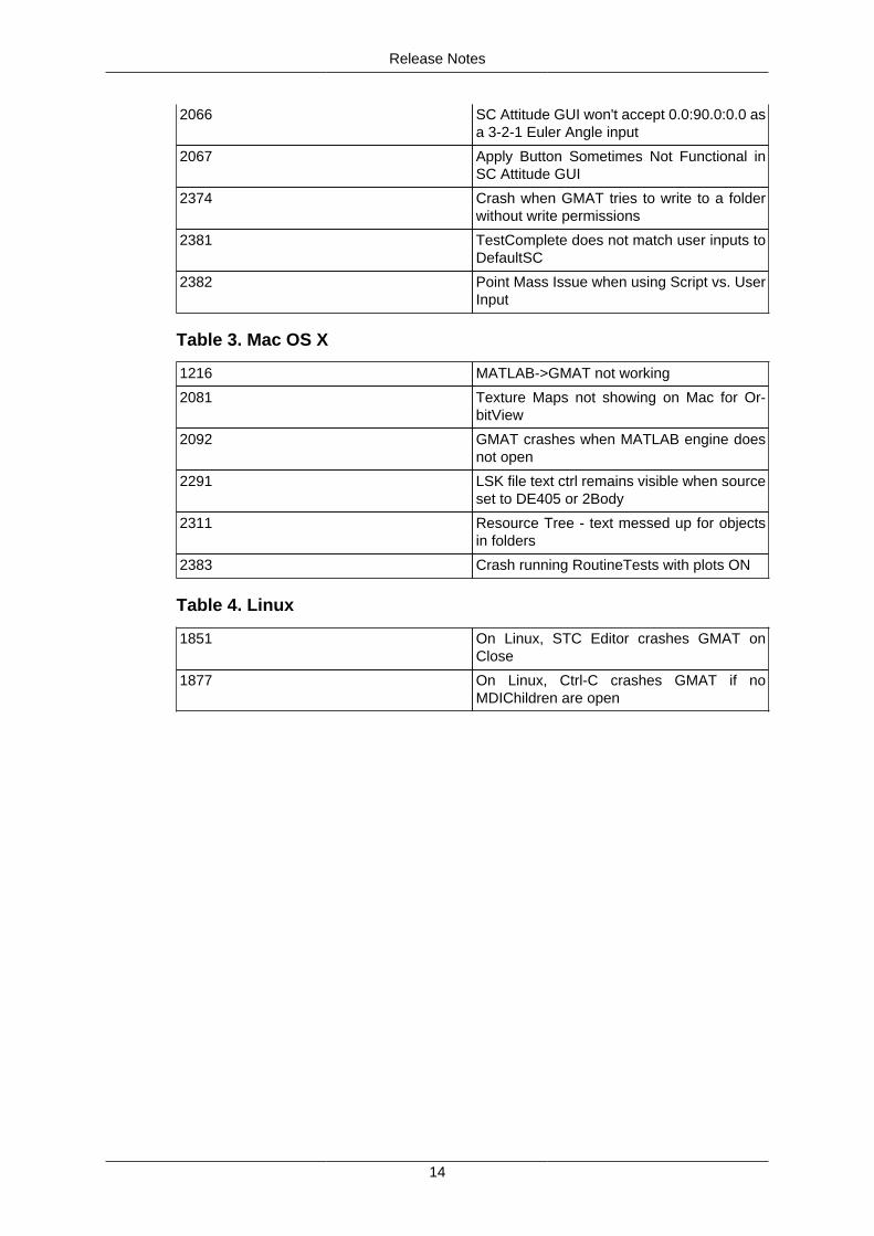
2066 SC Attitude GUI won't accept 0.0:90.0:0.0 asa 3-2-1 Euler Angle input
2067 Apply Button Sometimes Not Functional inSC Attitude GUI
2374 Crash when GMAT tries to write to a folderwithout write permissions
2381 TestComplete does not match user inputs toDefaultSC
2382 Point Mass Issue when using Script vs. UserInput
Table 3. Mac OS X
1216 MATLAB->GMAT not working
2081 Texture Maps not showing on Mac for Or-bitView
2092 GMAT crashes when MATLAB engine doesnot open
2291 LSK file text ctrl remains visible when sourceset to DE405 or 2Body
2311 Resource Tree - text messed up for objectsin folders
2383 Crash running RoutineTests with plots ON
Table 4. Linux
1851 On Linux, STC Editor crashes GMAT onClose
1877 On Linux, Ctrl-C crashes GMAT if noMDIChildren are open
15
How To
Reporting mission parameters
Running GMAT Scripts from MATLAB
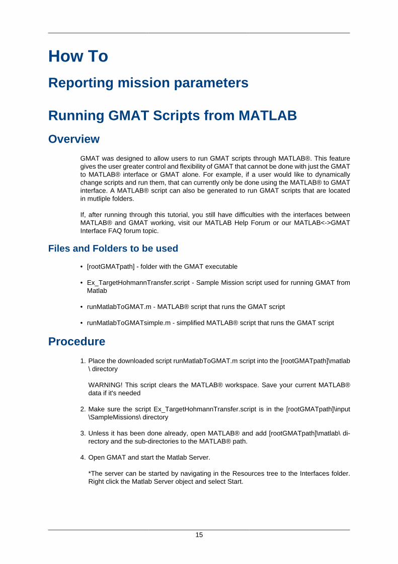
Overview
GMAT was designed to allow users to run GMAT scripts through MATLAB®. This featuregives the user greater control and flexibility of GMAT that cannot be done with just the GMATto MATLAB® interface or GMAT alone. For example, if a user would like to dynamicallychange scripts and run them, that can currently only be done using the MATLAB® to GMATinterface. A MATLAB® script can also be generated to run GMAT scripts that are locatedin mutliple folders.
If, after running through this tutorial, you still have difficulties with the interfaces betweenMATLAB® and GMAT working, visit our MATLAB Help Forum or our MATLAB<->GMATInterface FAQ forum topic.
Files and Folders to be used
• [rootGMATpath] - folder with the GMAT executable
• Ex_TargetHohmannTransfer.script - Sample Mission script used for running GMAT fromMatlab
• runMatlabToGMAT.m - MATLAB® script that runs the GMAT script
• runMatlabToGMATsimple.m - simplified MATLAB® script that runs the GMAT script
Procedure
1. Place the downloaded script runMatlabToGMAT.m script into the [rootGMATpath]\matlab\ directory
WARNING! This script clears the MATLAB® workspace. Save your current MATLAB®data if it's needed
2. Make sure the script Ex_TargetHohmannTransfer.script is in the [rootGMATpath]\input\SampleMissions\ directory
3. Unless it has been done already, open MATLAB® and add [rootGMATpath]\matlab\ di-rectory and the sub-directories to the MATLAB® path.
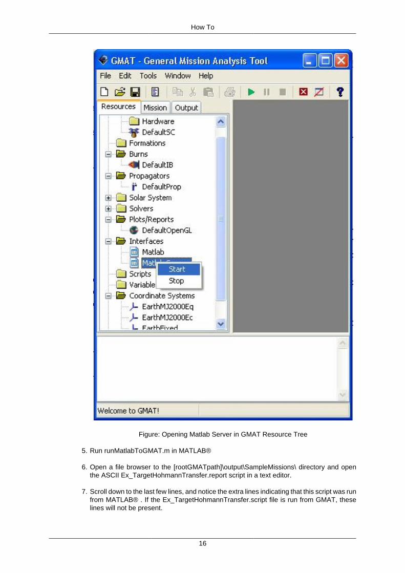
4. Open GMAT and start the Matlab Server.
*The server can be started by navigating in the Resources tree to the Interfaces folder.Right click the Matlab Server object and select Start.
How To
16
Figure: Opening Matlab Server in GMAT Resource Tree
5. Run runMatlabToGMAT.m in MATLAB®
6. Open a file browser to the [rootGMATpath]\output\SampleMissions\ directory and openthe ASCII Ex_TargetHohmannTransfer.report script in a text editor.
7. Scroll down to the last few lines, and notice the extra lines indicating that this script was runfrom MATLAB® . If the Ex_TargetHohmannTransfer.script file is run from GMAT, theselines will not be present.
How To
17
8. Congratulations - you have finished the main section of this tutorial. Be sure to open therunMatlabToGMAT.m script, to understand how GMAT is controlled by MATLAB® . ThisMATLAB® script is heavily commented to explain what is being done. If you still have ques-tions, feel free to post them at our GMAT Source Forge forums (http://sourceforge.net/projects/gmat/)
Additional Instructions
The runMatlabToGMAT.m Matlab script might be too complicated for novice MATLAB®users. If so, use a simplified version of the script, runMatlabToGMATsimple.m. For thisscript a .m file is needed, so copy the Ex_TargetHohmannTransfer.script and rename thecopy as Ex_TargetHohmannTransfer.m . Follow the above instructions but first rename therunMatlabToGMAT.m file to runMatlabToGMATsimple.m.
Creating ephemeris files
Creating a Report
Objective and Overview
The objective of this tutorial is to demonstrate how to report parameters out to a file usingtwo different reporting techniques, as well as how to use strings to improve the readabilityof a report file.
Download the script file: ReportFile.script
Prerequisites
• Objects modified (use if you have trouble with this tutorial):
• ReportFile
• Commands modified (use if you have trouble with this tutorial):
• Report Command
• ScriptEvent Command
Mission Description
• Objective: Use the Report Object to output parameters to an ascii file
• Assume: N/A
• Find: N/A
How To
18
Resource, Mission, and Output Trees
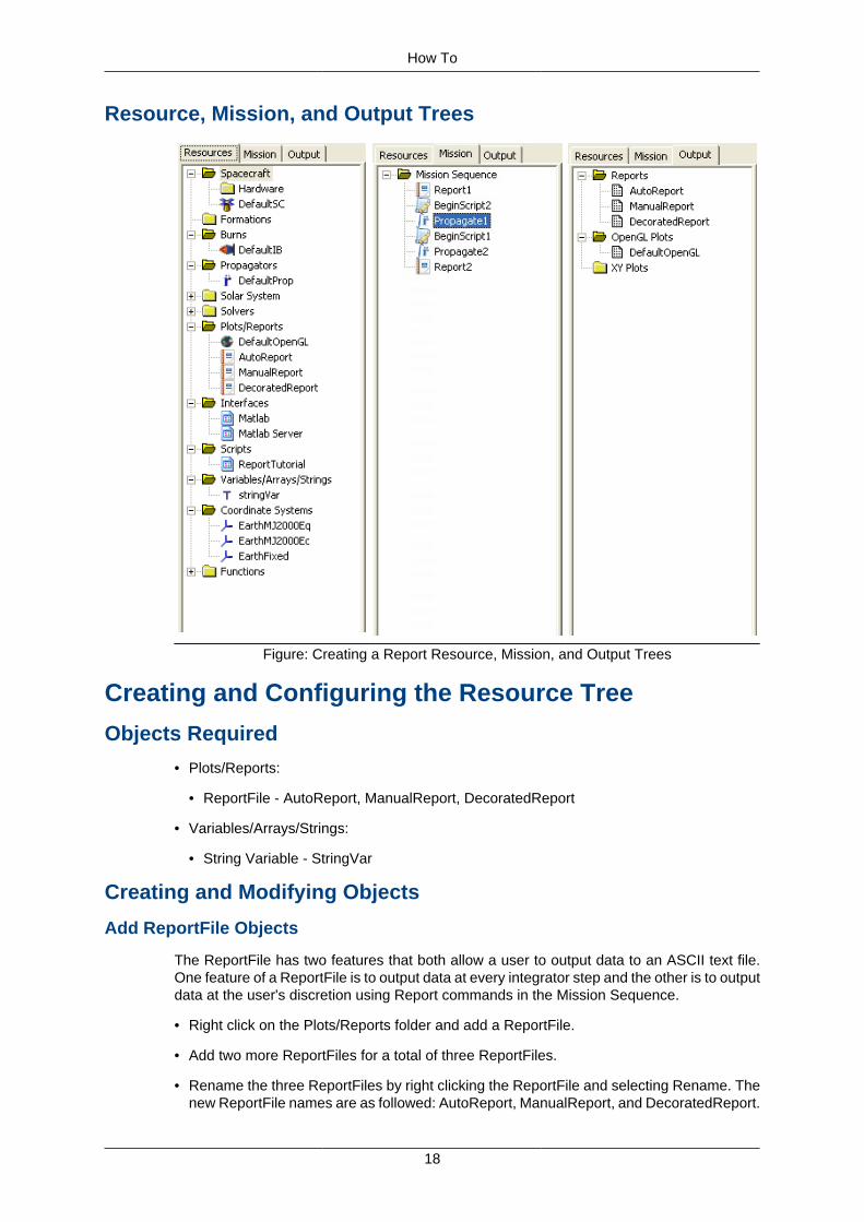
Figure: Creating a Report Resource, Mission, and Output Trees
Creating and Configuring the Resource Tree
Objects Required
• Plots/Reports:
• ReportFile - AutoReport, ManualReport, DecoratedReport
• Variables/Arrays/Strings:
• String Variable - StringVar
Creating and Modifying Objects
Add ReportFile Objects
The ReportFile has two features that both allow a user to output data to an ASCII text file.One feature of a ReportFile is to output data at every integrator step and the other is to outputdata at the user's discretion using Report commands in the Mission Sequence.
• Right click on the Plots/Reports folder and add a ReportFile.
• Add two more ReportFiles for a total of three ReportFiles.
• Rename the three ReportFiles by right clicking the ReportFile and selecting Rename. Thenew ReportFile names are as followed: AutoReport, ManualReport, and DecoratedReport.
How To
19
• Verify that your Plots/Reports Resource Tree settings are identical to the image below.
Figure: Plots/Reports Resource Tree Folder
Configure AutoReport ReportFile
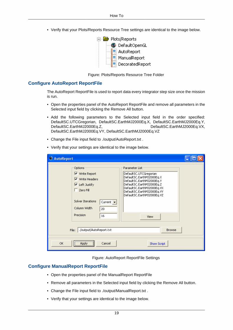
The AutoReport ReportFile is used to report data every integrator step size once the missionis run.
• Open the properties panel of the AutoReport ReportFile and remove all parameters in theSelected input field by clicking the Remove All button.
• Add the following parameters to the Selected input field in the order specified:DefaultSC.UTCGregorian, DefaultSC.EarthMJ2000Eq.X, DefaultSC.EarthMJ2000Eq.Y,DefaultSC.EarthMJ2000Eq.Z, DefaultSC.EarthMJ2000Eq.VX,DefaultSC.EarthMJ2000Eq.VY, DefaultSC.EarthMJ2000Eq.VZ
• Change the File input field to ./output/AutoReport.txt .
• Verify that your settings are identical to the image below.
Figure: AutoReport ReportFile Settings
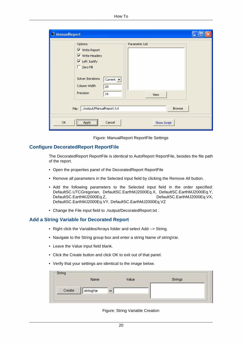
Configure ManualReport ReportFile
• Open the properties panel of the ManualReport ReportFile
• Remove all parameters in the Selected input field by clicking the Remove All button.
• Change the File input field to ./output/ManualReport.txt .
• Verify that your settings are identical to the image below.
How To
20
Figure: ManualReport ReportFile Settings
Configure DecoratedReport ReportFile
The DecoratedReport ReportFile is identical to AutoReport ReportFile, besides the file pathof the report.
• Open the properties panel of the DecoratedReport ReportFile
• Remove all parameters in the Selected input field by clicking the Remove All button.
• Add the following parameters to the Selected input field in the order specified:DefaultSC.UTCGregorian, DefaultSC.EarthMJ2000Eq.X, DefaultSC.EarthMJ2000Eq.Y,DefaultSC.EarthMJ2000Eq.Z, DefaultSC.EarthMJ2000Eq.VX,DefaultSC.EarthMJ2000Eq.VY, DefaultSC.EarthMJ2000Eq.VZ
• Change the File input field to ./output/DecoratedReport.txt .
Add a String Variable for Decorated Report
• Right click the Variables/Arrays folder and select Add --> String.
• Navigate to the String group box and enter a string Name of stringVar.
• Leave the Value input field blank.
• Click the Create button and click OK to exit out of that panel.
• Verify that your settings are identical to the image below.
Figure: String Variable Creation
How To
21
Creating and Configuring the Mission Tree
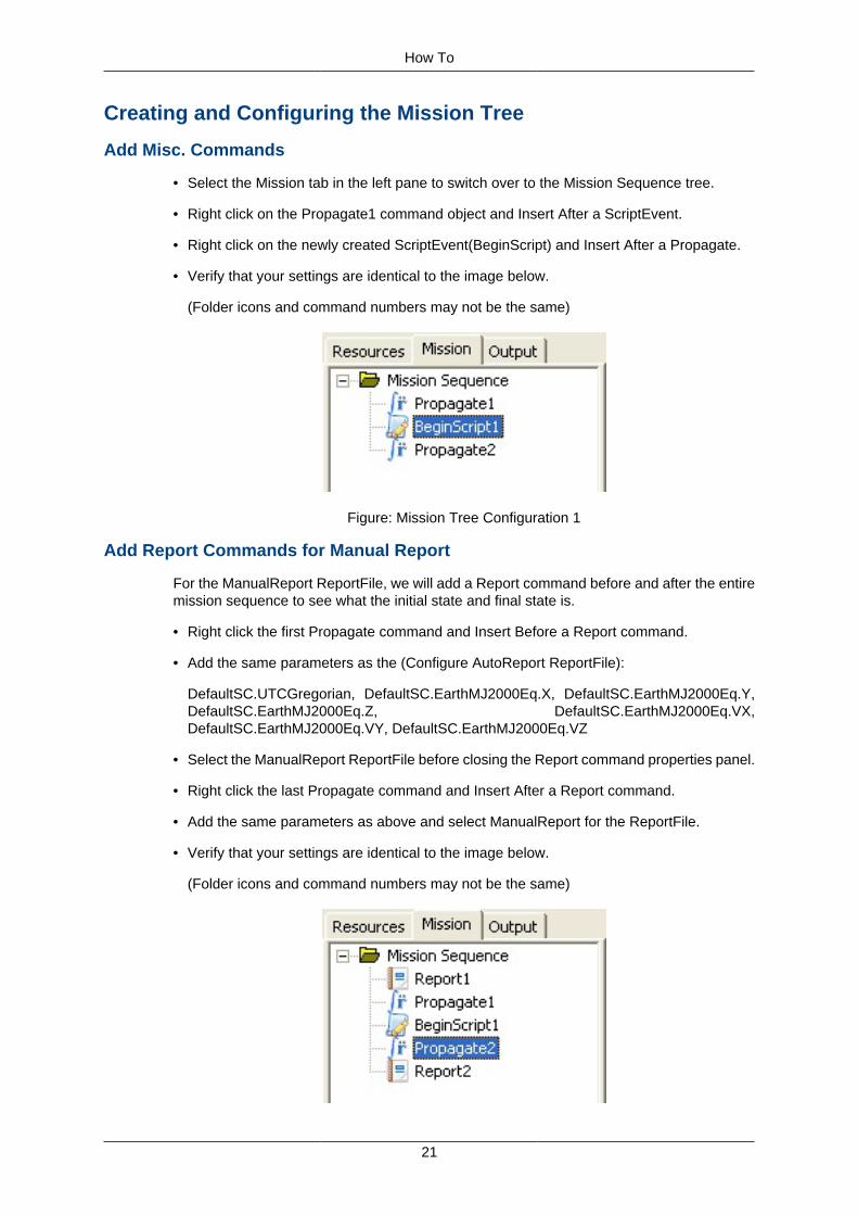
Add Misc. Commands
• Select the Mission tab in the left pane to switch over to the Mission Sequence tree.
• Right click on the Propagate1 command object and Insert After a ScriptEvent.
• Right click on the newly created ScriptEvent(BeginScript) and Insert After a Propagate.
• Verify that your settings are identical to the image below.
(Folder icons and command numbers may not be the same)
Figure: Mission Tree Configuration 1
Add Report Commands for Manual Report
For the ManualReport ReportFile, we will add a Report command before and after the entiremission sequence to see what the initial state and final state is.
• Right click the first Propagate command and Insert Before a Report command.
• Add the same parameters as the (Configure AutoReport ReportFile):
DefaultSC.UTCGregorian, DefaultSC.EarthMJ2000Eq.X, DefaultSC.EarthMJ2000Eq.Y,DefaultSC.EarthMJ2000Eq.Z, DefaultSC.EarthMJ2000Eq.VX,DefaultSC.EarthMJ2000Eq.VY, DefaultSC.EarthMJ2000Eq.VZ
• Select the ManualReport ReportFile before closing the Report command properties panel.
• Right click the last Propagate command and Insert After a Report command.
• Add the same parameters as above and select ManualReport for the ReportFile.
• Verify that your settings are identical to the image below.
(Folder icons and command numbers may not be the same)
How To
22
Figure: Mission Tree Configuration 2
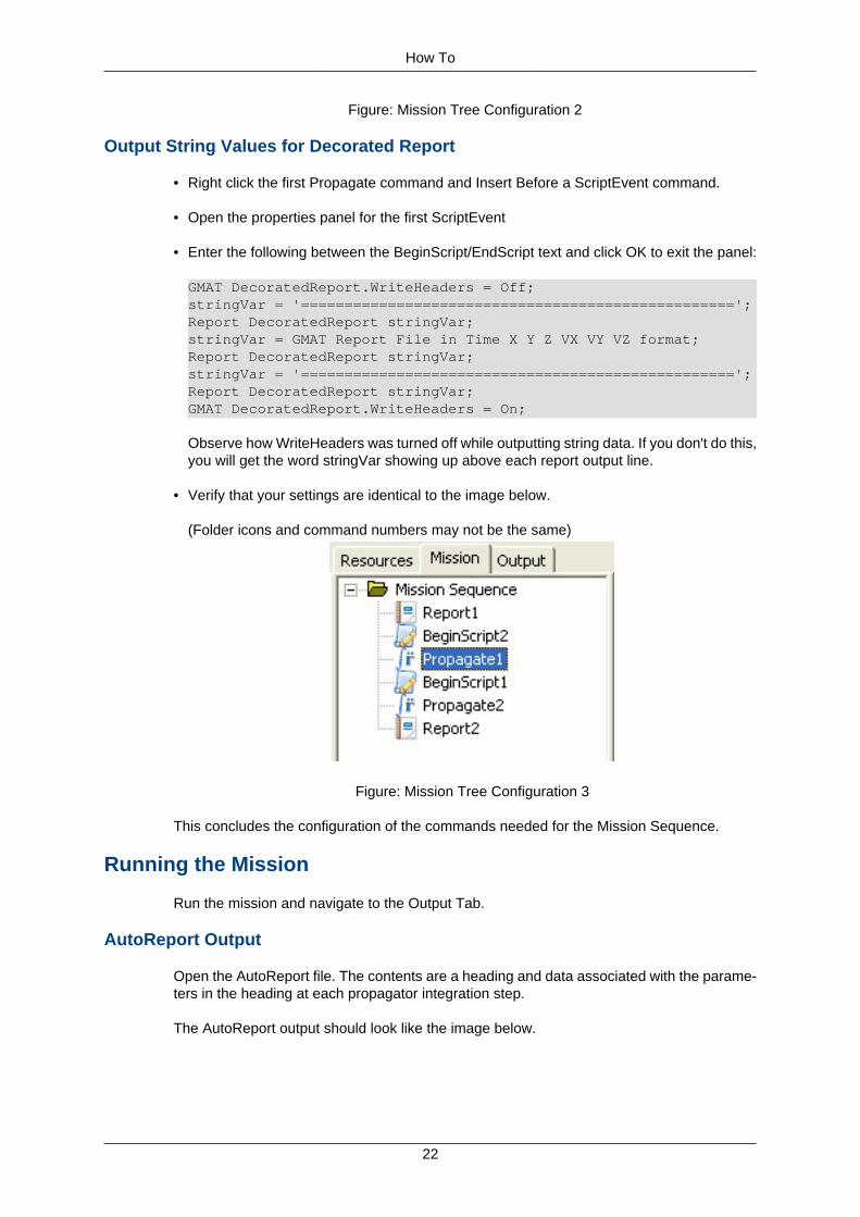
Output String Values for Decorated Report
• Right click the first Propagate command and Insert Before a ScriptEvent command.
• Open the properties panel for the first ScriptEvent
• Enter the following between the BeginScript/EndScript text and click OK to exit the panel:
GMAT DecoratedReport.WriteHeaders = Off;stringVar = '==================================================';Report DecoratedReport stringVar;stringVar = GMAT Report File in Time X Y Z VX VY VZ format;Report DecoratedReport stringVar;stringVar = '==================================================';Report DecoratedReport stringVar;GMAT DecoratedReport.WriteHeaders = On;
Observe how WriteHeaders was turned off while outputting string data. If you don't do this,you will get the word stringVar showing up above each report output line.
• Verify that your settings are identical to the image below.
(Folder icons and command numbers may not be the same)
Figure: Mission Tree Configuration 3
This concludes the configuration of the commands needed for the Mission Sequence.
Running the Mission
Run the mission and navigate to the Output Tab.
AutoReport Output
Open the AutoReport file. The contents are a heading and data associated with the parame-ters in the heading at each propagator integration step.
The AutoReport output should look like the image below.
How To
23
Figure: AutoReport Output Results
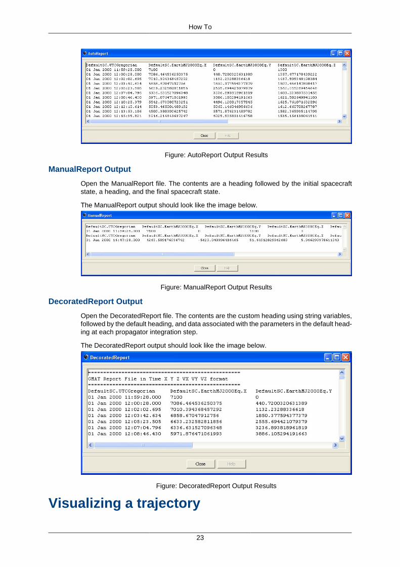
ManualReport Output
Open the ManualReport file. The contents are a heading followed by the initial spacecraftstate, a heading, and the final spacecraft state.
The ManualReport output should look like the image below.
Figure: ManualReport Output Results
DecoratedReport Output
Open the DecoratedReport file. The contents are the custom heading using string variables,followed by the default heading, and data associated with the parameters in the default head-ing at each propagator integration step.
The DecoratedReport output should look like the image below.
Figure: DecoratedReport Output Results
Visualizing a trajectory
24
Samples and TutorialsPropagating a Spacecraft
Objective and OverviewThe objective of this tutorial is to teach you how to create a spacecraft and a propagator, andthen propagate the spacecraft to orbit perigee by following these basic steps:
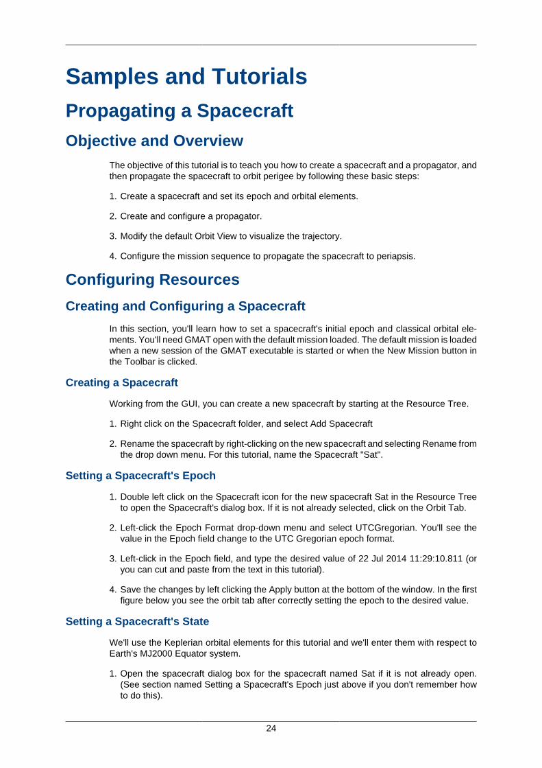
1. Create a spacecraft and set its epoch and orbital elements.
2. Create and configure a propagator.
3. Modify the default Orbit View to visualize the trajectory.
4. Configure the mission sequence to propagate the spacecraft to periapsis.
Configuring Resources
Creating and Configuring a Spacecraft
In this section, you'll learn how to set a spacecraft's initial epoch and classical orbital ele-ments. You'll need GMAT open with the default mission loaded. The default mission is loadedwhen a new session of the GMAT executable is started or when the New Mission button inthe Toolbar is clicked.
Creating a Spacecraft
Working from the GUI, you can create a new spacecraft by starting at the Resource Tree.
1. Right click on the Spacecraft folder, and select Add Spacecraft
2. Rename the spacecraft by right-clicking on the new spacecraft and selecting Rename fromthe drop down menu. For this tutorial, name the Spacecraft "Sat".
Setting a Spacecraft's Epoch
1. Double left click on the Spacecraft icon for the new spacecraft Sat in the Resource Treeto open the Spacecraft's dialog box. If it is not already selected, click on the Orbit Tab.
2. Left-click the Epoch Format drop-down menu and select UTCGregorian. You'll see thevalue in the Epoch field change to the UTC Gregorian epoch format.
3. Left-click in the Epoch field, and type the desired value of 22 Jul 2014 11:29:10.811 (oryou can cut and paste from the text in this tutorial).
4. Save the changes by left clicking the Apply button at the bottom of the window. In the firstfigure below you see the orbit tab after correctly setting the epoch to the desired value.
Setting a Spacecraft's State
We'll use the Keplerian orbital elements for this tutorial and we'll enter them with respect toEarth's MJ2000 Equator system.
1. Open the spacecraft dialog box for the spacecraft named Sat if it is not already open.(See section named Setting a Spacecraft's Epoch just above if you don't remember howto do this).
Samples and Tutorials
25
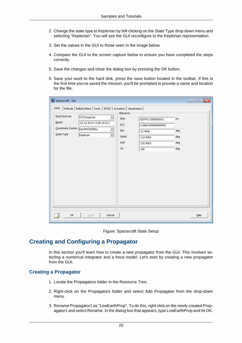
2. Change the state type to Keplerian by left-clicking on the State Type drop down menu andselecting "Keplerian". You will see the GUI reconfigure to the Keplerian representation.
3. Set the values in the GUI to those seen in the image below.
4. Compare the GUI to the screen capture below to ensure you have completed the stepscorrectly.
5. Save the changes and close the dialog box by pressing the OK button.
6. Save your work to the hard disk, press the save button located in the toolbar. If this isthe first time you've saved the mission, you'll be prompted to provide a name and locationfor the file.
Figure: Spacecraft State Setup
Creating and Configuring a Propagator
In this section you'll learn how to create a new propagator from the GUI. This involves se-lecting a numerical integrator and a force model. Let's start by creating a new propagatorfrom the GUI.
Creating a Propagator
1. Locate the Propagators folder in the Resource Tree.
2. Right-click on the Propagators folder and select Add Propagator from the drop-downmenu.
3. Rename Propagator1 as "LowEarthProp". To do this, right click on the newly created Prop-agator1 and select Rename. In the dialog box that appears, type LowEarthProp and hit OK.
Samples and Tutorials
26
Look at the dialog box for LowEarthProp by double left clicking on its icon under the Propa-gators folder. On the left side of the propagator dialog box you see where you can select thedesired numerical integrator and configure it for your application. On the right hand side ofthe panel are combo boxes and lists that allow the user to set up the force model. Now let'slook at how to configure a force model.
Configuring a Force Model
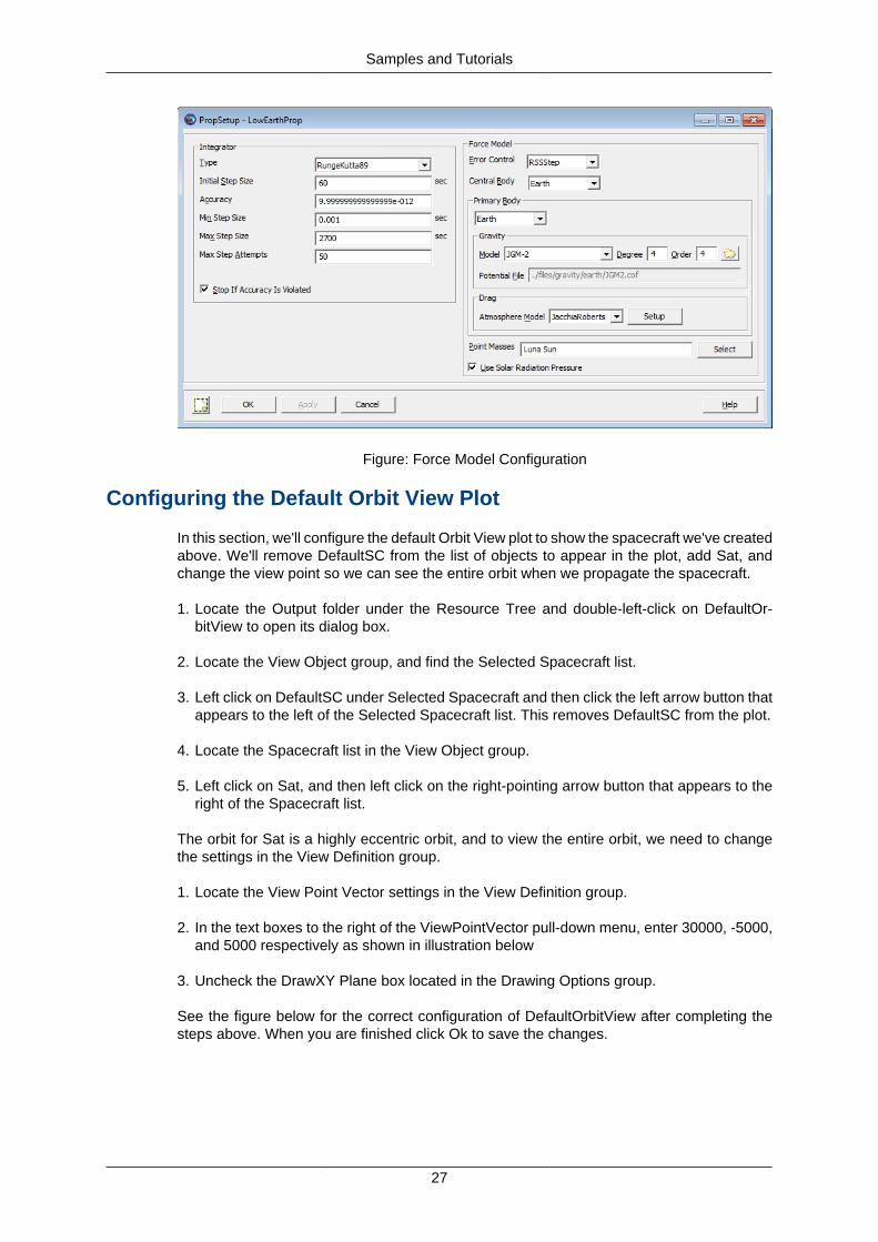
For this tutorial we will use an Earth 10x10 non-spherical gravity model, Jacchia-Robertsatmospheric model, and point mass perturbations from the Sun and Moon.
1. Open LowEarthProp from the Propagators folder in the Resource tree
2. Locate the Primary Bodies group on the Propagator dialog box. In the Gravity group box,change the degree and order to 10 by left clicking in the text field and typing in the values.
3. Locate the Atmosphere Model pull-down menu in the Drag group.
4. Left click on the pull-down menu and select JacchiaRoberts. (For now we will leave thedefault options for Jacchia-Roberts model)
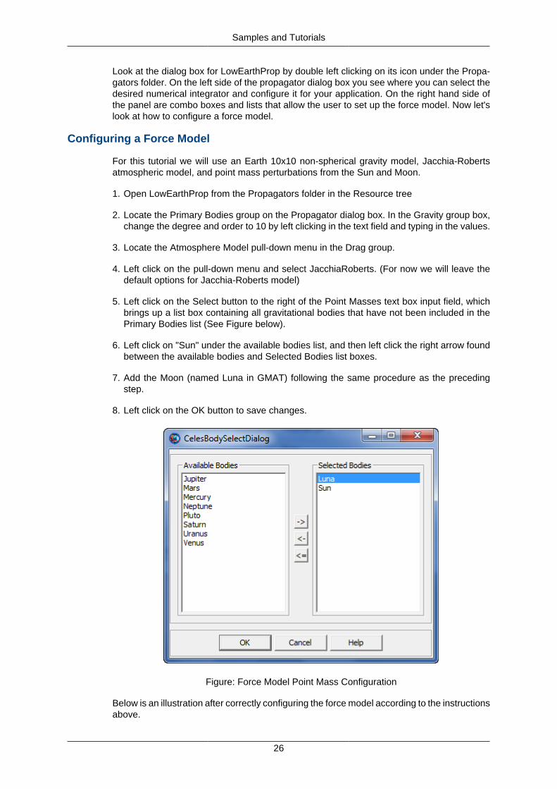
5. Left click on the Select button to the right of the Point Masses text box input field, whichbrings up a list box containing all gravitational bodies that have not been included in thePrimary Bodies list (See Figure below).
6. Left click on "Sun" under the available bodies list, and then left click the right arrow foundbetween the available bodies and Selected Bodies list boxes.
7. Add the Moon (named Luna in GMAT) following the same procedure as the precedingstep.
8. Left click on the OK button to save changes.
Figure: Force Model Point Mass Configuration
Below is an illustration after correctly configuring the force model according to the instructionsabove.
Samples and Tutorials
27
Figure: Force Model Configuration
Configuring the Default Orbit View Plot
In this section, we'll configure the default Orbit View plot to show the spacecraft we've createdabove. We'll remove DefaultSC from the list of objects to appear in the plot, add Sat, andchange the view point so we can see the entire orbit when we propagate the spacecraft.
1. Locate the Output folder under the Resource Tree and double-left-click on DefaultOr-bitView to open its dialog box.
2. Locate the View Object group, and find the Selected Spacecraft list.
3. Left click on DefaultSC under Selected Spacecraft and then click the left arrow button thatappears to the left of the Selected Spacecraft list. This removes DefaultSC from the plot.
4. Locate the Spacecraft list in the View Object group.
5. Left click on Sat, and then left click on the right-pointing arrow button that appears to theright of the Spacecraft list.
The orbit for Sat is a highly eccentric orbit, and to view the entire orbit, we need to changethe settings in the View Definition group.
1. Locate the View Point Vector settings in the View Definition group.
2. In the text boxes to the right of the ViewPointVector pull-down menu, enter 30000, -5000,and 5000 respectively as shown in illustration below
3. Uncheck the DrawXY Plane box located in the Drawing Options group.
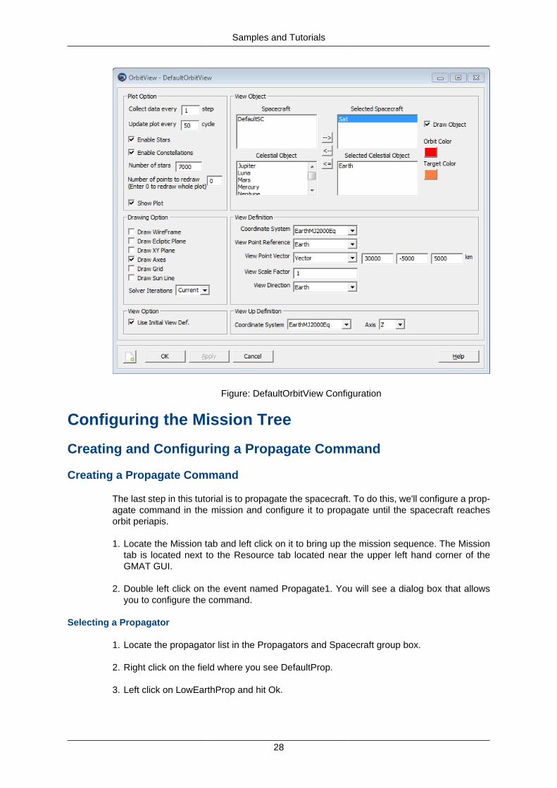
See the figure below for the correct configuration of DefaultOrbitView after completing thesteps above. When you are finished click Ok to save the changes.
Samples and Tutorials
28
Figure: DefaultOrbitView Configuration
Configuring the Mission Tree
Creating and Configuring a Propagate Command
Creating a Propagate Command
The last step in this tutorial is to propagate the spacecraft. To do this, we'll configure a prop-agate command in the mission and configure it to propagate until the spacecraft reachesorbit periapis.
1. Locate the Mission tab and left click on it to bring up the mission sequence. The Missiontab is located next to the Resource tab located near the upper left hand corner of theGMAT GUI.
2. Double left click on the event named Propagate1. You will see a dialog box that allowsyou to configure the command.
Selecting a Propagator
1. Locate the propagator list in the Propagators and Spacecraft group box.
2. Right click on the field where you see DefaultProp.
3. Left click on LowEarthProp and hit Ok.
Samples and Tutorials
29
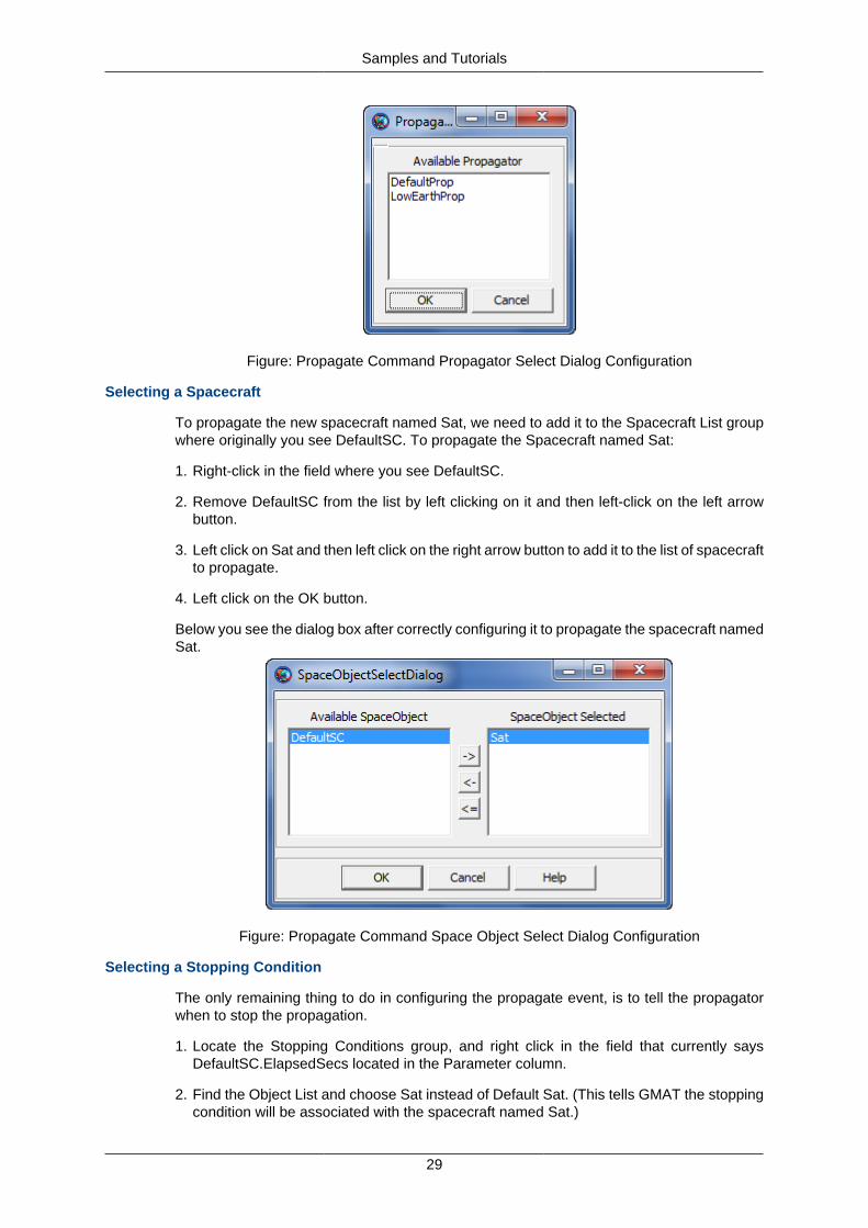
Figure: Propagate Command Propagator Select Dialog Configuration
Selecting a Spacecraft
To propagate the new spacecraft named Sat, we need to add it to the Spacecraft List groupwhere originally you see DefaultSC. To propagate the Spacecraft named Sat:
1. Right-click in the field where you see DefaultSC.
2. Remove DefaultSC from the list by left clicking on it and then left-click on the left arrowbutton.
3. Left click on Sat and then left click on the right arrow button to add it to the list of spacecraftto propagate.
4. Left click on the OK button.
Below you see the dialog box after correctly configuring it to propagate the spacecraft namedSat.
Figure: Propagate Command Space Object Select Dialog Configuration
Selecting a Stopping Condition
The only remaining thing to do in configuring the propagate event, is to tell the propagatorwhen to stop the propagation.
1. Locate the Stopping Conditions group, and right click in the field that currently saysDefaultSC.ElapsedSecs located in the Parameter column.
2. Find the Object List and choose Sat instead of Default Sat. (This tells GMAT the stoppingcondition will be associated with the spacecraft named Sat.)
Samples and Tutorials
30
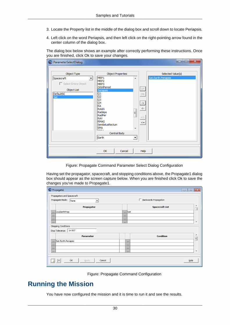
3. Locate the Property list in the middle of the dialog box and scroll down to locate Periapsis.
4. Left click on the word Periapsis, and then left click on the right-pointing arrow found in thecenter column of the dialog box.
The dialog box below shows an example after correctly performing these instructions. Onceyou are finished, click Ok to save your changes.
Figure: Propagate Command Parameter Select Dialog Configuration
Having set the propagator, spacecraft, and stopping conditions above, the Propagate1 dialogbox should appear as the screen capture below. When you are finished click Ok to save thechanges you've made to Propagate1.
Figure: Propagate Command Configuration
Running the MissionYou have now configured the mission and it is time to run it and see the results.
Samples and Tutorials
31
1. Left-click on the Save button in the toolbar.
2. Left-click on the Run button in the toolbar.
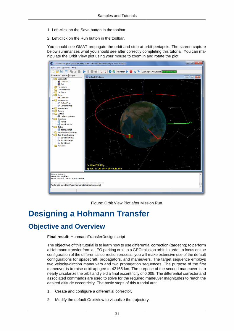
You should see GMAT propagate the orbit and stop at orbit periapsis. The screen capturebelow summarizes what you should see after correctly completing this tutorial. You can ma-nipulate the Orbit View plot using your mouse to zoom in and rotate the plot.
Figure: Orbit View Plot after Mission Run
Designing a Hohmann Transfer
Objective and OverviewFinal result: HohmannTransferDesign.script
The objective of this tutorial is to learn how to use differential correction (targeting) to performa Hohmann transfer from a LEO parking orbit to a GEO mission orbit. In order to focus on theconfiguration of the differential correction process, you will make extensive use of the defaultconfigurations for spacecraft, propagators, and maneuvers. The target sequence employstwo velocity-dirction maneuvers and two propagation sequences. The purpose of the firstmaneuver is to raise orbit apogee to 42165 km. The purpose of the second maneuver is tonearly circularize the orbit and yield a final eccentricity of 0.005. The differential corrector andassociated commands are used to solve for the required maneuver magnitudes to reach thedesired altitude eccentricity. The basic steps of this tutorial are:
1. Create and configure a differential corrector.
2. Modify the default OrbitView to visualize the trajectory.
Samples and Tutorials
32
3. Create two default impulsive maneuvers.
4. Add a target sequence to the mission to raise apogee to GEO altitude and circularizethe orbit.
5. Run the mission, save the solution, and rerun the mission using the converged solution.
Creating and Configuring the Resource Tree
Begin by loading the default mission ( click the new mission button in the toolbar) or startinga new GMAT session. For this tutorial, we will use the default configurations for a spaceraft(DefaultSC), a propagator (DefaultProp), and maneuvers. DefaultSC is configured to a nearcircular orbit and DefaultProp is configured to use Earth as the central body with a gravitymodel of degree and order 4. The default impulsive burn model uses the Velocity NormalBinormal (VNB) coordinate system. You may want to open the dialog boxes for these objectsand inspect them more closely as we will leave the settings of those objects at their defaultvalues.
Creating the Differential Corrector
To create a differential corrector:
1. Locate the Solvers folder in the Resource Tree and expand it if it is minimized.
2. Right-click the Boundary Value Solvers folder, select Add, and then select Differential-Corrector.
Modifying the default Orbit View
You need to make minor modifications to default Orbit View so that the entire final orbit willfit in the graphics window.
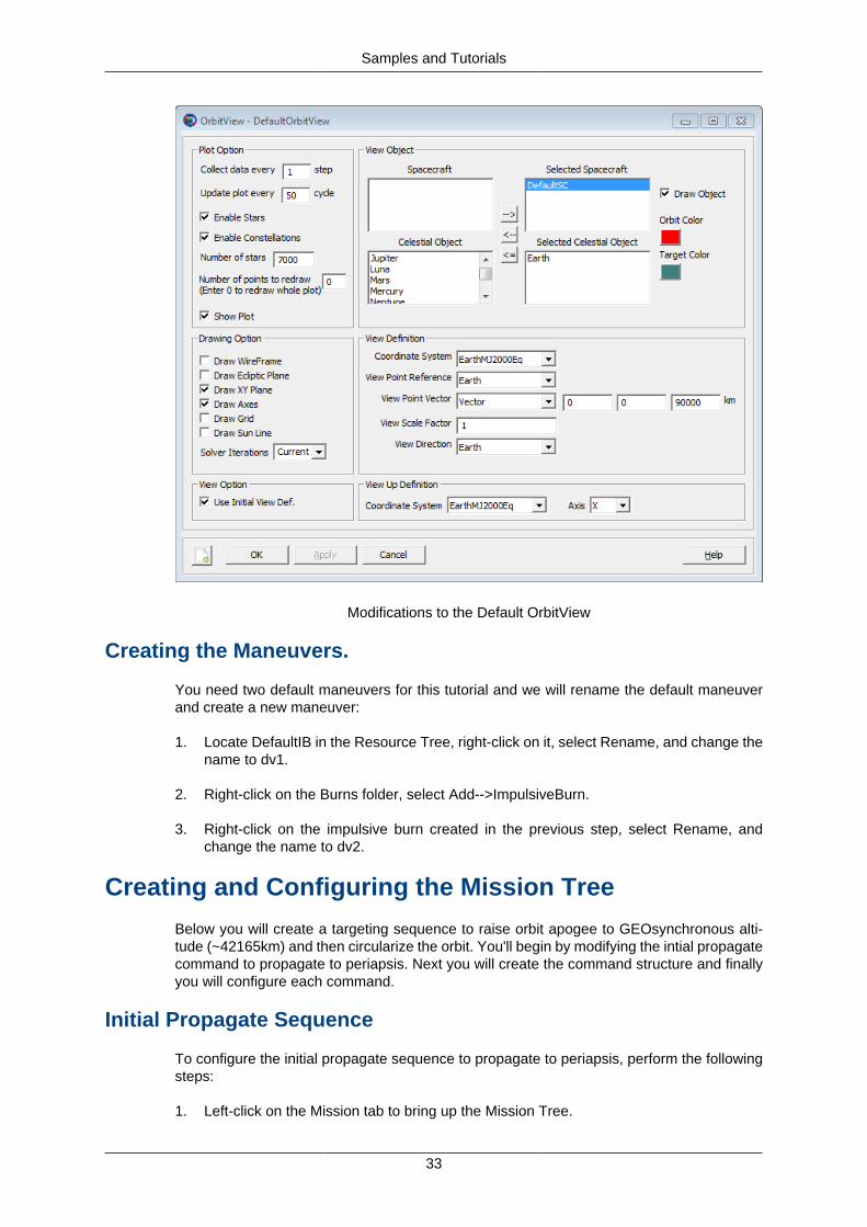
1. Locate DefaultOrbitView in the Resource Tree, right-click on it, and select Open.
2. Change the SolverIterations input field, located in the Drawing Option group box, to thevalue Current.
3. Change ViewPointVector to 0, 0, 90000 respectively.
4. Change the ViewUpDefinition Axis to X.
5. Verify the configuration against the screen capture below, make any changes necessary,and click Ok on the DefaultOrbitView dialog box.
Samples and Tutorials
33
Modifications to the Default OrbitView
Creating the Maneuvers.
You need two default maneuvers for this tutorial and we will rename the default maneuverand create a new maneuver:
1. Locate DefaultIB in the Resource Tree, right-click on it, select Rename, and change thename to dv1.
2. Right-click on the Burns folder, select Add-->ImpulsiveBurn.
3. Right-click on the impulsive burn created in the previous step, select Rename, andchange the name to dv2.
Creating and Configuring the Mission Tree
Below you will create a targeting sequence to raise orbit apogee to GEOsynchronous alti-tude (~42165km) and then circularize the orbit. You'll begin by modifying the intial propagatecommand to propagate to periapsis. Next you will create the command structure and finallyyou will configure each command.
Initial Propagate Sequence
To configure the initial propagate sequence to propagate to periapsis, perform the followingsteps:
1. Left-click on the Mission tab to bring up the Mission Tree.
Samples and Tutorials
34
2. Right-click on Propagate1 and select Open from the menu.
3. Locate the Stopping Conditions group box and then right click on the set of ellipses nextto the text "DefaultSC.ElapsedSecs". This will open the Parameter Select Dialog box.
4. Under the Object Properties list on the Parameter Select Dialog box, locate periapsisand double-click on it. Click the Ok button to close the Parameter Select Dialog box.
5. Click the Ok button on the Propagate 1 dialog box to save changes and close.
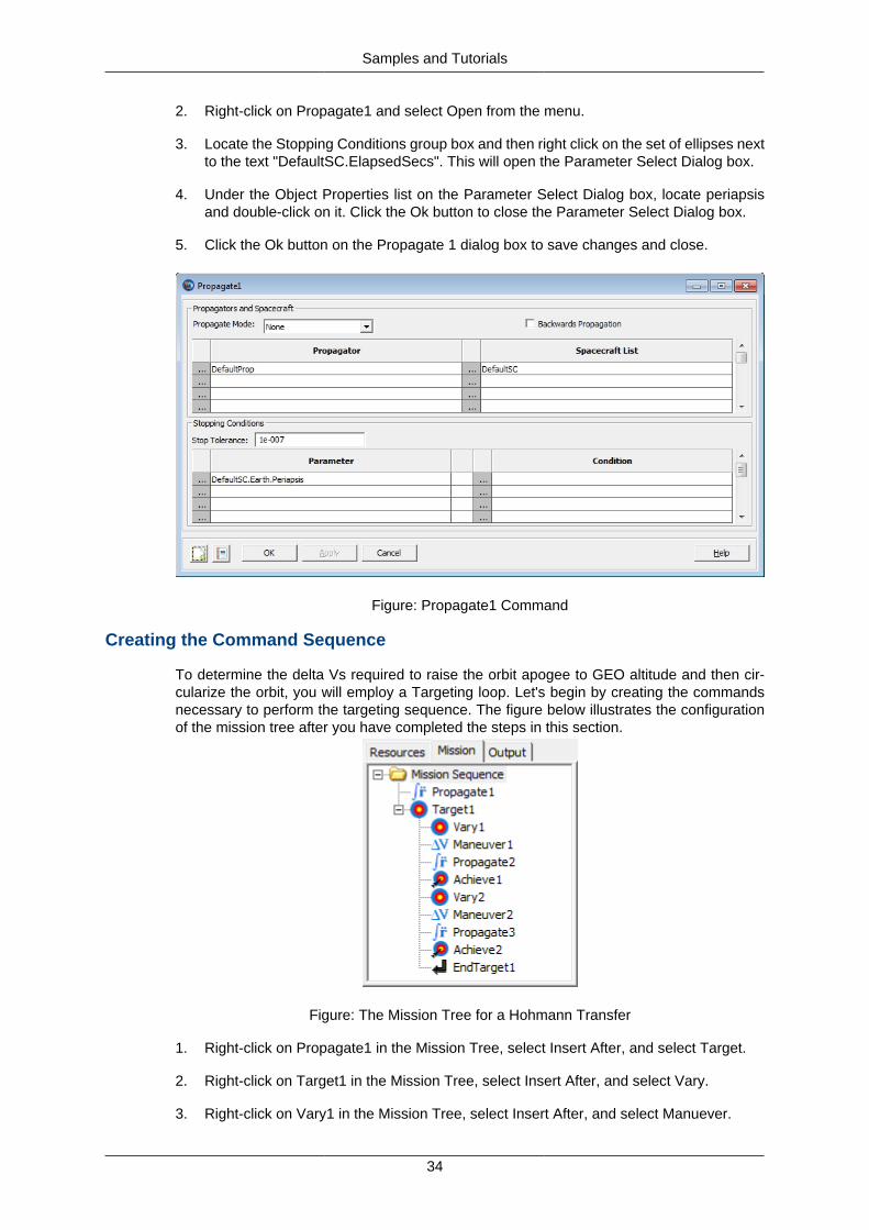
Figure: Propagate1 Command
Creating the Command Sequence
To determine the delta Vs required to raise the orbit apogee to GEO altitude and then cir-cularize the orbit, you will employ a Targeting loop. Let's begin by creating the commandsnecessary to perform the targeting sequence. The figure below illustrates the configurationof the mission tree after you have completed the steps in this section.
Figure: The Mission Tree for a Hohmann Transfer
1. Right-click on Propagate1 in the Mission Tree, select Insert After, and select Target.
2. Right-click on Target1 in the Mission Tree, select Insert After, and select Vary.
3. Right-click on Vary1 in the Mission Tree, select Insert After, and select Manuever.
Samples and Tutorials
35
4. Right-click on Maneuver1 in the Mission Tree, select Insert After, and select Propagate.
5. Right-click on Propagate2 in the Mission Tree, select Insert After, and select Achieve.
6. Right-click on Achieve1 in the Mission Tree, select Insert After, and select Vary.
7. Right-click on Vary2 in the Mission Tree, select Insert After, and select Manuever.
8. Right-click on Maneuver2 in the Mission Tree, select Insert After, and select Propagate.
9. Right-click on Propagate3 in the Mission Tree, select Insert After, and select Achieve.
Let's talk about the function of the command sequence you created above. The Vary com-mands define the variables the differential corrector can modify to achieve the goals de-fined in the Achieve commands. Because there are two variables (Vary commands) and twoAchieve commands (constraints), this is a "square" targeting problem. Below you will con-figure the Vary commands to modify the maneuver values to achieve a final orbit radius of42165 and an eccentricity of 0.005
Configuring the Command Sequence
Now you will configure the commands you created above to solve for the delta-Vs requiredto perform a Hohmann transfer.
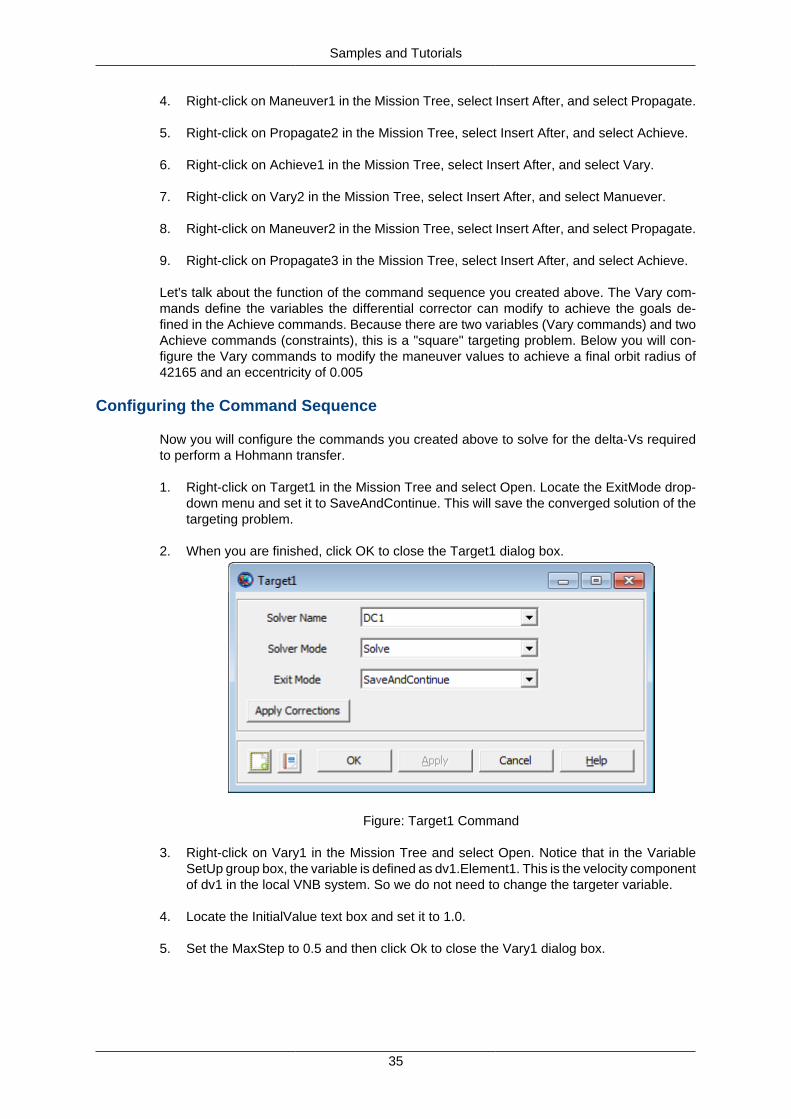
1. Right-click on Target1 in the Mission Tree and select Open. Locate the ExitMode drop-down menu and set it to SaveAndContinue. This will save the converged solution of thetargeting problem.
2. When you are finished, click OK to close the Target1 dialog box.
Figure: Target1 Command
3. Right-click on Vary1 in the Mission Tree and select Open. Notice that in the VariableSetUp group box, the variable is defined as dv1.Element1. This is the velocity componentof dv1 in the local VNB system. So we do not need to change the targeter variable.
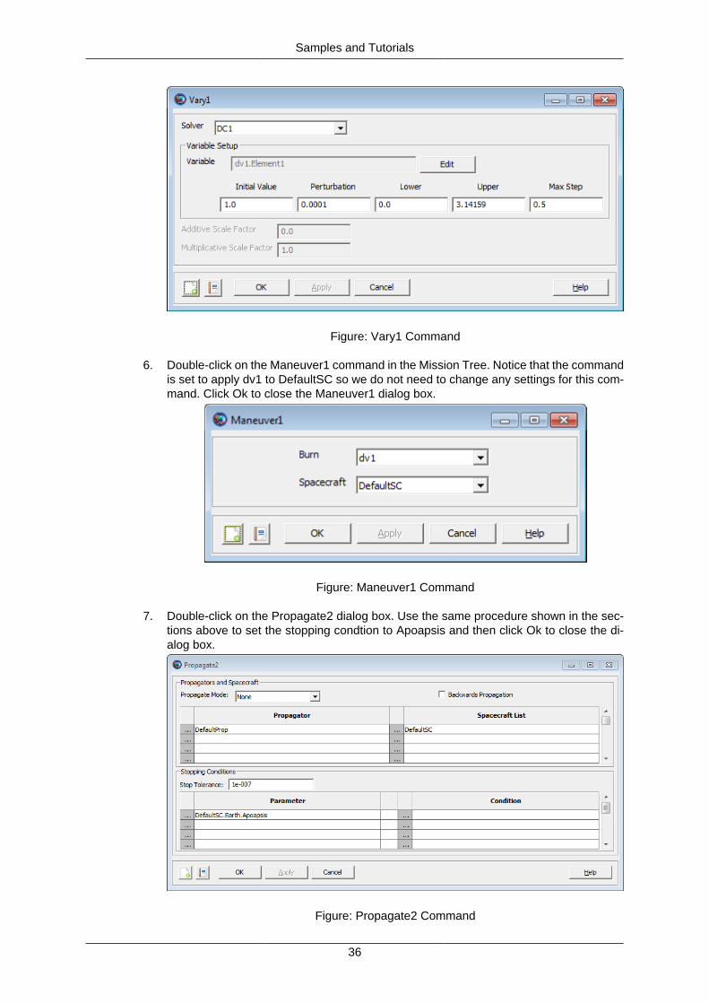
4. Locate the InitialValue text box and set it to 1.0.
5. Set the MaxStep to 0.5 and then click Ok to close the Vary1 dialog box.
Samples and Tutorials
36
Figure: Vary1 Command
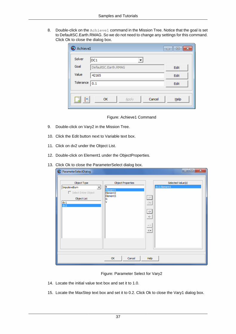
6. Double-click on the Maneuver1 command in the Mission Tree. Notice that the commandis set to apply dv1 to DefaultSC so we do not need to change any settings for this com-mand. Click Ok to close the Maneuver1 dialog box.
Figure: Maneuver1 Command
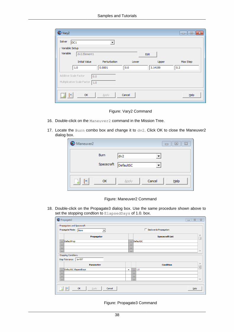
7. Double-click on the Propagate2 dialog box. Use the same procedure shown in the sec-tions above to set the stopping condtion to Apoapsis and then click Ok to close the di-alog box.
Figure: Propagate2 Command
Samples and Tutorials
37
8. Double-click on the Achieve1 command in the Mission Tree. Notice that the goal is setto DefaultSC.Earth.RMAG. So we do not need to change any settings for this command.Click Ok to close the dialog box.
Figure: Achieve1 Command
9. Double-click on Vary2 in the Mission Tree.
10. Click the Edit button next to Variable text box.
11. Click on dv2 under the Object List.
12. Double-click on Element1 under the ObjectProperties.
13. Click Ok to close the ParameterSelect dialog box.
Figure: Parameter Select for Vary2
14. Locate the initial value text box and set it to 1.0.
15. Locate the MaxStep text box and set it to 0.2. Click Ok to close the Vary1 dialog box.
Samples and Tutorials
38
Figure: Vary2 Command
16. Double-click on the Maneuver2 command in the Mission Tree.
17. Locate the Burn combo box and change it to dv2. Click OK to close the Maneuver2dialog box.
Figure: Maneuver2 Command
18. Double-click on the Propagate3 dialog box. Use the same procedure shown above toset the stopping condtion to ElapsedDays of 1.0. box.
Figure: Propagate3 Command
Samples and Tutorials
39
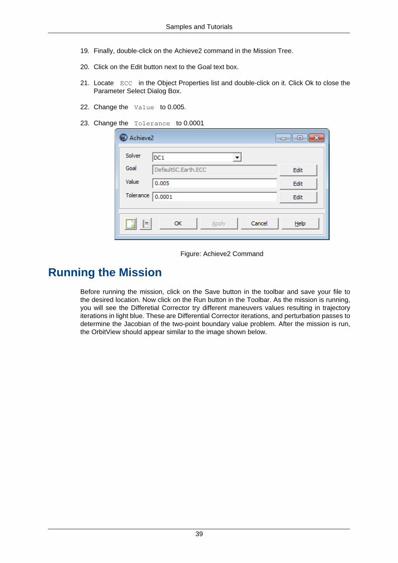
19. Finally, double-click on the Achieve2 command in the Mission Tree.
20. Click on the Edit button next to the Goal text box.
21. Locate ECC in the Object Properties list and double-click on it. Click Ok to close theParameter Select Dialog Box.
22. Change the Value to 0.005.
23. Change the Tolerance to 0.0001
Figure: Achieve2 Command
Running the Mission
Before running the mission, click on the Save button in the toolbar and save your file tothe desired location. Now click on the Run button in the Toolbar. As the mission is running,you will see the Differetial Corrector try different maneuvers values resulting in trajectoryiterations in light blue. These are Differential Corrector iterations, and perturbation passes todetermine the Jacobian of the two-point boundary value problem. After the mission is run,the OrbitView should appear similar to the image shown below.
Samples and Tutorials
40
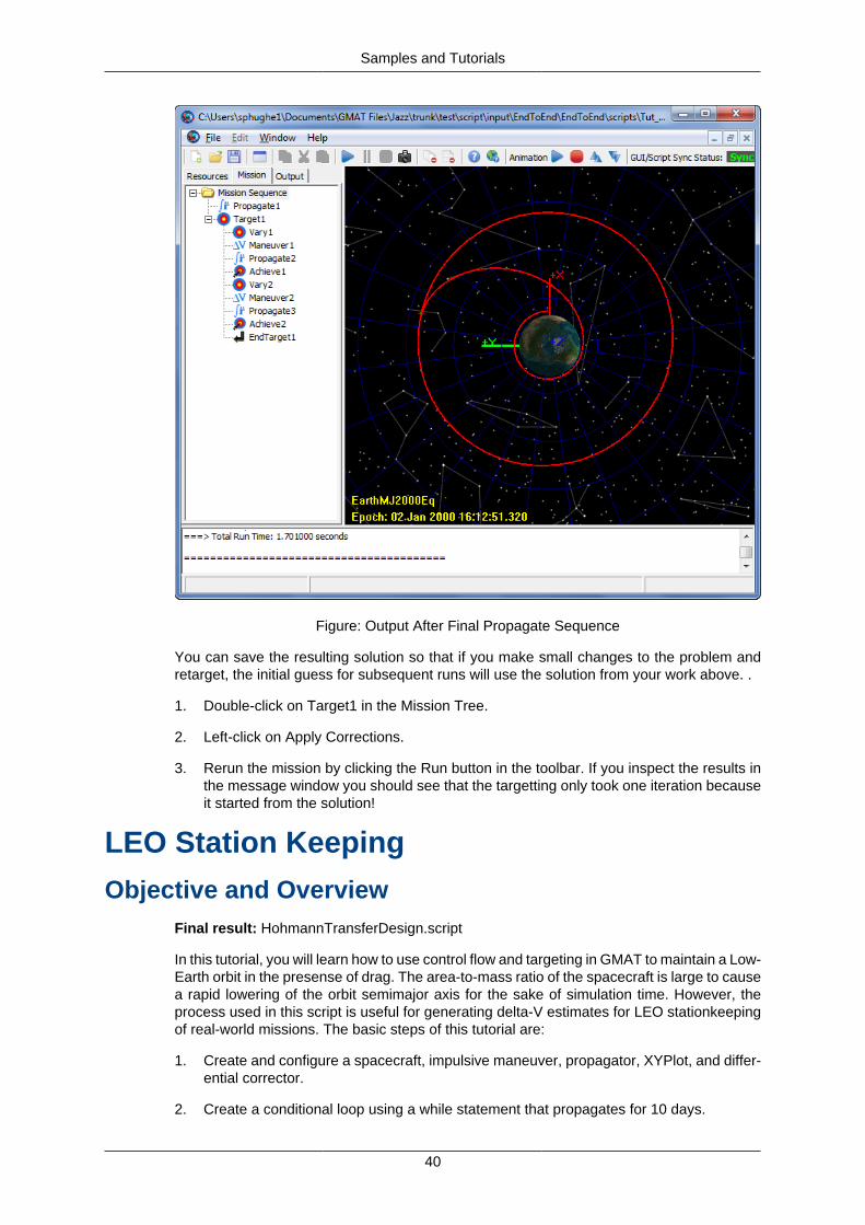
Figure: Output After Final Propagate Sequence
You can save the resulting solution so that if you make small changes to the problem andretarget, the initial guess for subsequent runs will use the solution from your work above. .
1. Double-click on Target1 in the Mission Tree.
2. Left-click on Apply Corrections.
3. Rerun the mission by clicking the Run button in the toolbar. If you inspect the results inthe message window you should see that the targetting only took one iteration becauseit started from the solution!
LEO Station Keeping
Objective and OverviewFinal result: HohmannTransferDesign.script
In this tutorial, you will learn how to use control flow and targeting in GMAT to maintain a Low-Earth orbit in the presense of drag. The area-to-mass ratio of the spacecraft is large to causea rapid lowering of the orbit semimajor axis for the sake of simulation time. However, theprocess used in this script is useful for generating delta-V estimates for LEO stationkeepingof real-world missions. The basic steps of this tutorial are:
1. Create and configure a spacecraft, impulsive maneuver, propagator, XYPlot, and differ-ential corrector.
2. Create a conditional loop using a while statement that propagates for 10 days.
Samples and Tutorials
41
3. Run the mission and observe the behavior if there is no orbit control strategy.
4. Create a target sequence nested in an if statement that executes if altitude is below342 km.
5. Run the mission and observe the behavior of orbit altitude with the control strategy im-plemented in step 4.
Creating and Configuring the Resource TreeIn this section, you will configure a model of a LEO spacecraft, a propopagator , a maneuver,and an XY plot to visualize the SMA during the control sequence developed in the nextsection.
Creating the Spacecraft
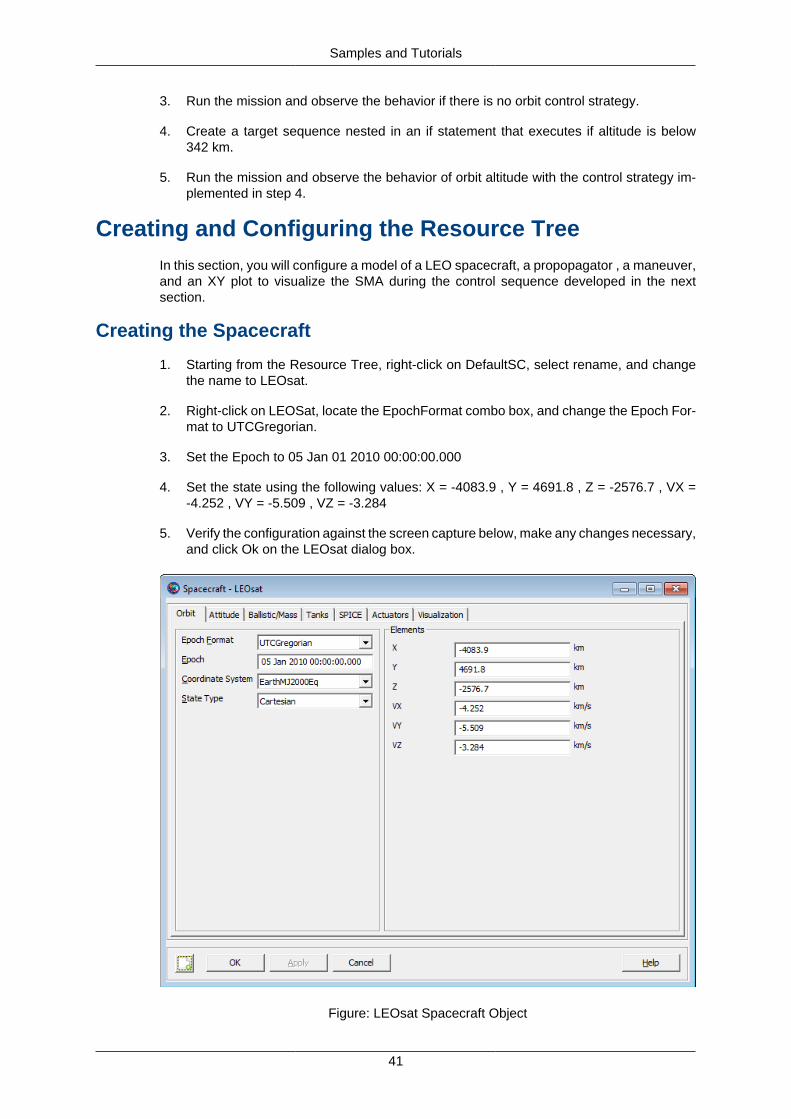
1. Starting from the Resource Tree, right-click on DefaultSC, select rename, and changethe name to LEOsat.
2. Right-click on LEOSat, locate the EpochFormat combo box, and change the Epoch For-mat to UTCGregorian.
3. Set the Epoch to 05 Jan 01 2010 00:00:00.000
4. Set the state using the following values: X = -4083.9 , Y = 4691.8 , Z = -2576.7 , VX =-4.252 , VY = -5.509 , VZ = -3.284
5. Verify the configuration against the screen capture below, make any changes necessary,and click Ok on the LEOsat dialog box.
Figure: LEOsat Spacecraft Object
Samples and Tutorials
42
Creating the Propagator
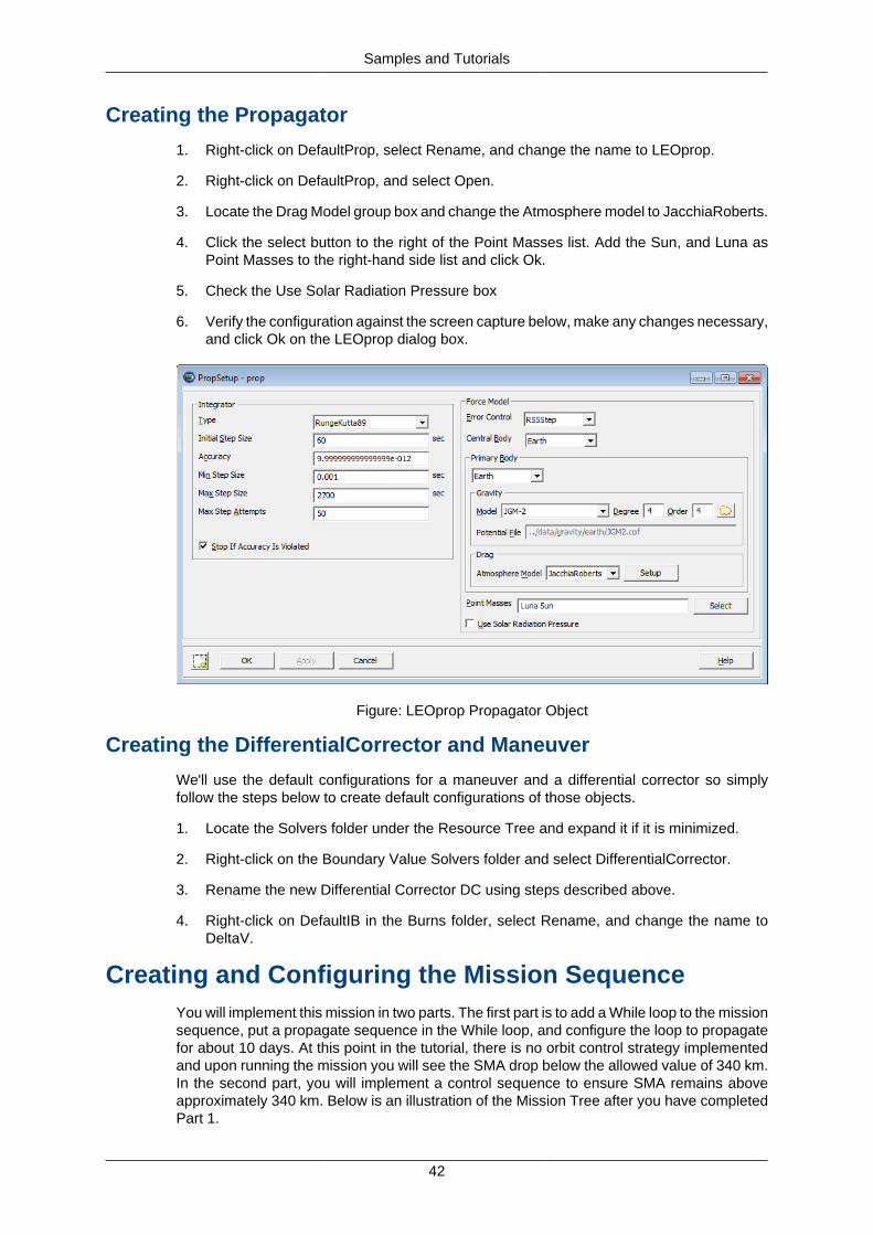
1. Right-click on DefaultProp, select Rename, and change the name to LEOprop.
2. Right-click on DefaultProp, and select Open.
3. Locate the Drag Model group box and change the Atmosphere model to JacchiaRoberts.
4. Click the select button to the right of the Point Masses list. Add the Sun, and Luna asPoint Masses to the right-hand side list and click Ok.
5. Check the Use Solar Radiation Pressure box
6. Verify the configuration against the screen capture below, make any changes necessary,and click Ok on the LEOprop dialog box.
Figure: LEOprop Propagator Object
Creating the DifferentialCorrector and Maneuver
We'll use the default configurations for a maneuver and a differential corrector so simplyfollow the steps below to create default configurations of those objects.
1. Locate the Solvers folder under the Resource Tree and expand it if it is minimized.
2. Right-click on the Boundary Value Solvers folder and select DifferentialCorrector.
3. Rename the new Differential Corrector DC using steps described above.
4. Right-click on DefaultIB in the Burns folder, select Rename, and change the name toDeltaV.
Creating and Configuring the Mission SequenceYou will implement this mission in two parts. The first part is to add a While loop to the missionsequence, put a propagate sequence in the While loop, and configure the loop to propagatefor about 10 days. At this point in the tutorial, there is no orbit control strategy implementedand upon running the mission you will see the SMA drop below the allowed value of 340 km.In the second part, you will implement a control sequence to ensure SMA remains aboveapproximately 340 km. Below is an illustration of the Mission Tree after you have completedPart 1.
Samples and Tutorials
43
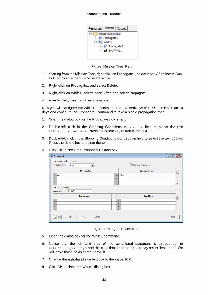
Figure: Mission Tree, Part I
1. Starting from the Mission Tree, right-click on Propagate1, select Insert After, locate Con-trol Logic in the menu, and select While.
2. Right-click on Propagate1 and select Delete.
3. Right-click on While1, select Insert After, and select Propagate.
4. After While1, insert another Propagate
Now you will configure the While1 to continue if the ElapsedDays of LEOsat is less than 10days and configure the Propagate2 command to take a single propagation step.
1. Open the dialog box for the Propagate1 command.
2. Double-left click in the Stopping Conditions Parameter field to select the textLEOSat.ElapsedSecs. Press the delete key to delete the text.
3. Double-left click in the Stopping Conditions Condition field to select the text 12000.Press the delete key to delete the text.
4. Click OK to close the Propagate1 dialog box.
Figure: Propagate1 Command
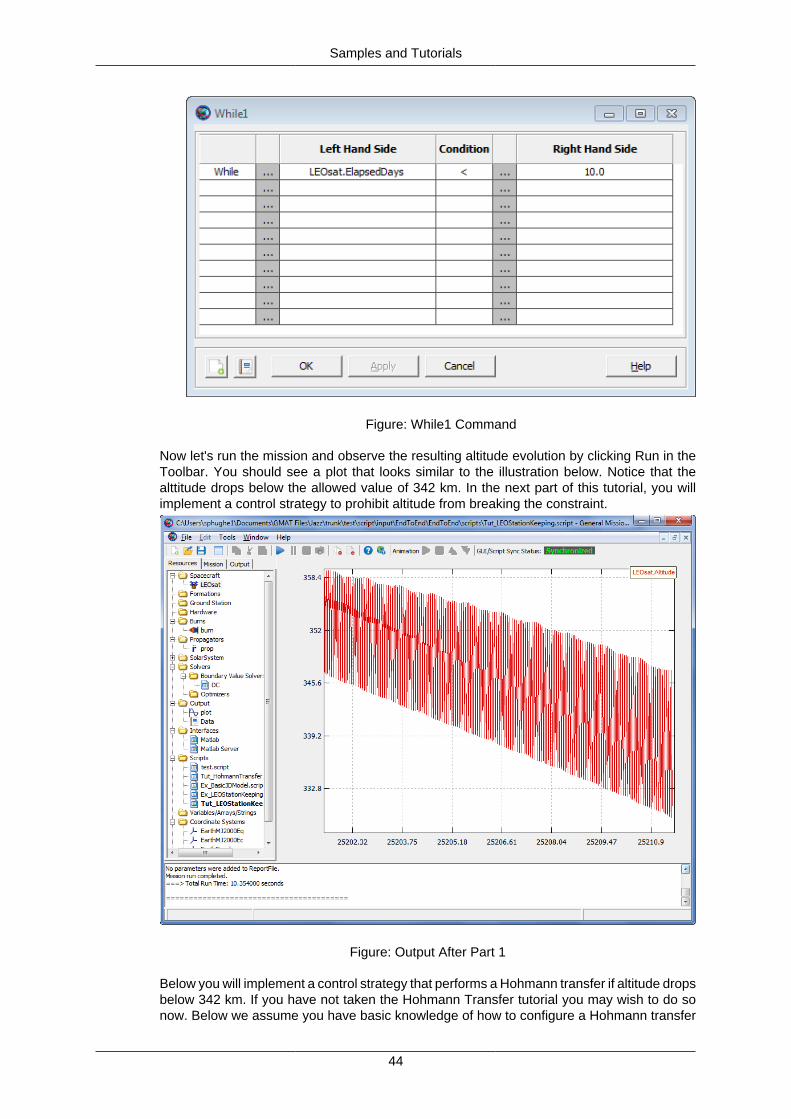
5. Open the dialog box for the While1 command.
6. Notice that the left-hand side of the conditional statement is already set toLEOSat.ElapsedDays and the conditional operator is already set to "less-than". Wewill leave those fields at their default.
7. Change the right-hand side text box to the value 10.0.
8. Click OK to close the While1 dialog box.
Samples and Tutorials
44
Figure: While1 Command
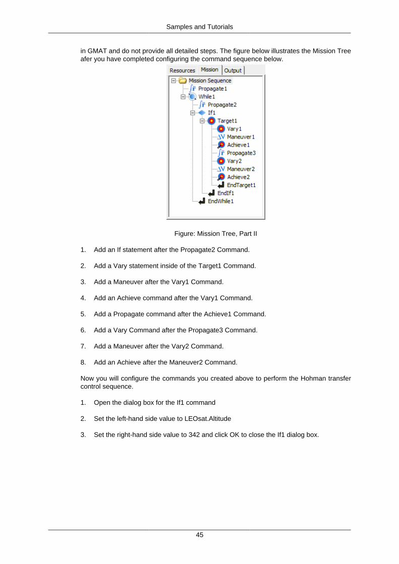
Now let's run the mission and observe the resulting altitude evolution by clicking Run in theToolbar. You should see a plot that looks similar to the illustration below. Notice that thealttitude drops below the allowed value of 342 km. In the next part of this tutorial, you willimplement a control strategy to prohibit altitude from breaking the constraint.
Figure: Output After Part 1
Below you will implement a control strategy that performs a Hohmann transfer if altitude dropsbelow 342 km. If you have not taken the Hohmann Transfer tutorial you may wish to do sonow. Below we assume you have basic knowledge of how to configure a Hohmann transfer
Samples and Tutorials
45
in GMAT and do not provide all detailed steps. The figure below illustrates the Mission Treeafer you have completed configuring the command sequence below.
Figure: Mission Tree, Part II
1. Add an If statement after the Propagate2 Command.
2. Add a Vary statement inside of the Target1 Command.
3. Add a Maneuver after the Vary1 Command.
4. Add an Achieve command after the Vary1 Command.
5. Add a Propagate command after the Achieve1 Command.
6. Add a Vary Command after the Propagate3 Command.
7. Add a Maneuver after the Vary2 Command.
8. Add an Achieve after the Maneuver2 Command.
Now you will configure the commands you created above to perform the Hohman transfercontrol sequence.
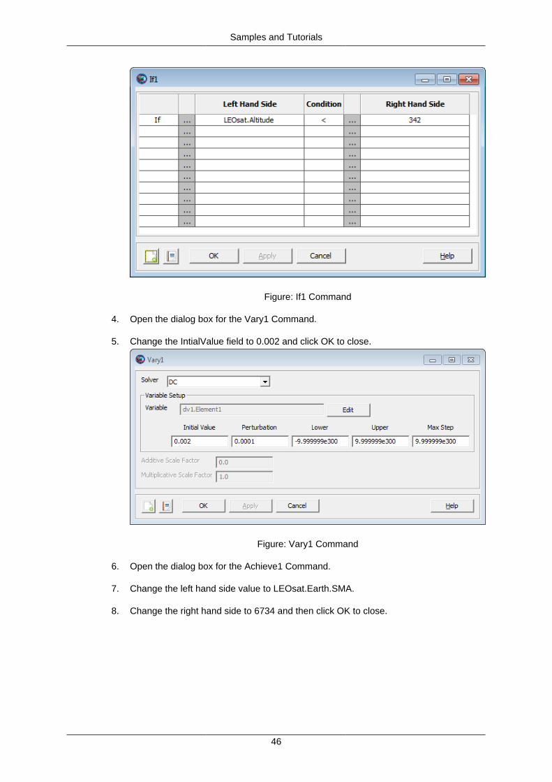
1. Open the dialog box for the If1 command
2. Set the left-hand side value to LEOsat.Altitude
3. Set the right-hand side value to 342 and click OK to close the If1 dialog box.
Samples and Tutorials
46
Figure: If1 Command
4. Open the dialog box for the Vary1 Command.
5. Change the IntialValue field to 0.002 and click OK to close.
Figure: Vary1 Command
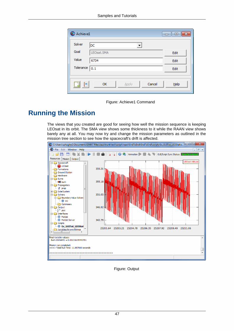
6. Open the dialog box for the Achieve1 Command.
7. Change the left hand side value to LEOsat.Earth.SMA.
8. Change the right hand side to 6734 and then click OK to close.
Samples and Tutorials
47
Figure: Achieve1 Command
Running the Mission
The views that you created are good for seeing how well the mission sequence is keepingLEOsat in its orbit. The SMA view shows some thickness to it while the RAAN view showsbarely any at all. You may now try and change the mission parameters as outlined in themission tree section to see how the spacecraft's drift is affected.
Figure: Output
Samples and Tutorials
48
Algebraic Optimization
Objective and Overview
This tutorial finds the minimum value to satisfy a function. This tutorial is intended to showhow GMAT's optimizer works. Uses of optimization in a true mission include minimizing theamount of fuel or minimum flight time required to achieve certain characteristics. Learninghow to optimize a mission sequence also involves learning about optimizers, nonlinear con-straints, and the minimize command.
You can download the script file and run it beforehand to see the final results of this tutorial:Ex_AlgebraicOptimization.script
Prerequisites
• Basic Understanding of how to create and propagate a spacecraft, as in Tutorial Creatingand Propagating a Spacecraft
Mission Description
• Objective: The goal here is to find values of variables X1 and X2 that minimize a criterionfunction F, with a constraint that X1+X2=8, as follows:
F = ( X1 - 2 )2 + ( X2 - 2 )2
G = X1 + X2
G = 8
• Find: Values X1 and X2
Creating and Configuring the Resource Tree
Objects Required
• Optimizer: SQPfmincon
• Plots/Reports: Report Data
• Variables: X1, X2, F, G
Creating and Modifying Objects
• Variables/Strings/Arrays
• Variable X1 = 0
• Variable X2 = 0
• Variable F = 0
• Variable G = 0
• Solvers
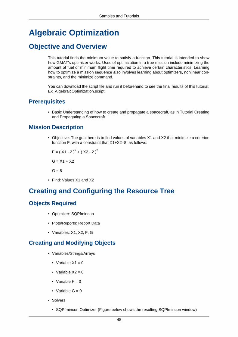
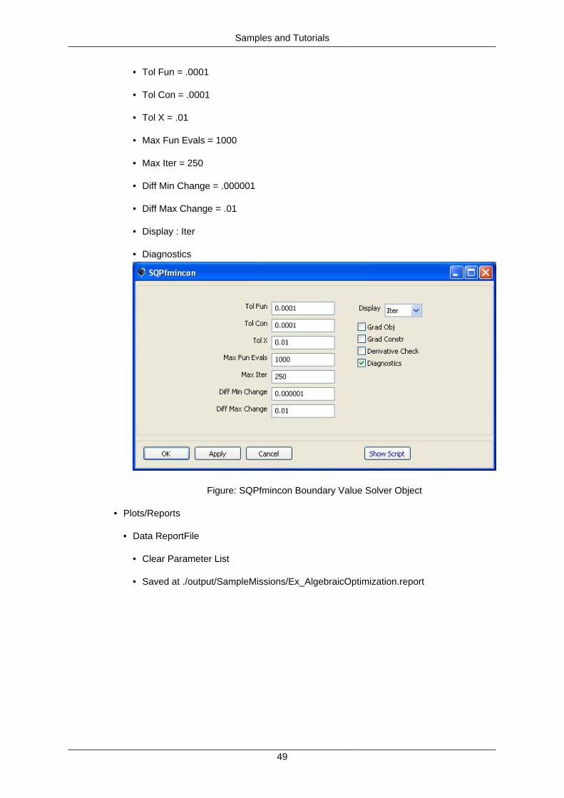
• SQPfmincon Optimizer (Figure below shows the resulting SQPfmincon window)
Samples and Tutorials
49
• Tol Fun = .0001
• Tol Con = .0001
• Tol X = .01
• Max Fun Evals = 1000
• Max Iter = 250
• Diff Min Change = .000001
• Diff Max Change = .01
• Display : Iter
• Diagnostics
Figure: SQPfmincon Boundary Value Solver Object
• Plots/Reports
• Data ReportFile
• Clear Parameter List
• Saved at ./output/SampleMissions/Ex_AlgebraicOptimization.report
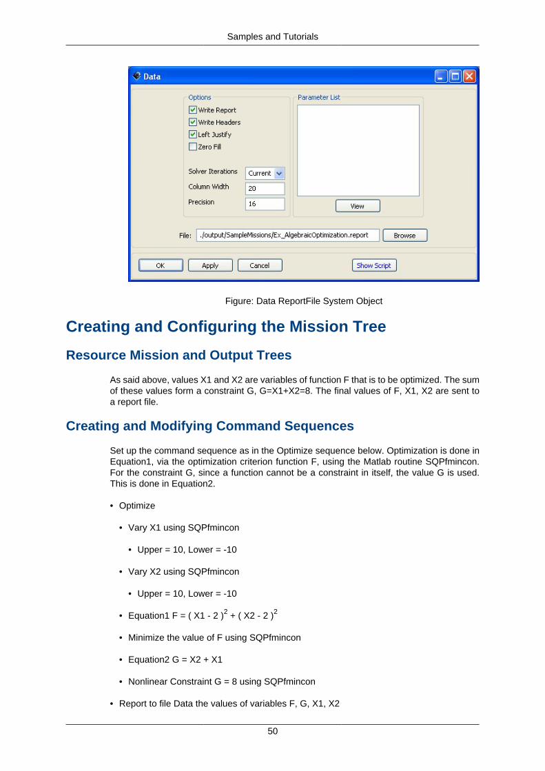
Samples and Tutorials
50
Figure: Data ReportFile System Object
Creating and Configuring the Mission Tree
Resource Mission and Output Trees
As said above, values X1 and X2 are variables of function F that is to be optimized. The sumof these values form a constraint G, G=X1+X2=8. The final values of F, X1, X2 are sent toa report file.
Creating and Modifying Command Sequences
Set up the command sequence as in the Optimize sequence below. Optimization is done inEquation1, via the optimization criterion function F, using the Matlab routine SQPfmincon.For the constraint G, since a function cannot be a constraint in itself, the value G is used.This is done in Equation2.
• Optimize
• Vary X1 using SQPfmincon
• Upper = 10, Lower = -10
• Vary X2 using SQPfmincon
• Upper = 10, Lower = -10
• Equation1 F = ( X1 - 2 )2 + ( X2 - 2 )2
• Minimize the value of F using SQPfmincon
• Equation2 G = X2 + X1
• Nonlinear Constraint G = 8 using SQPfmincon
• Report to file Data the values of variables F, G, X1, X2
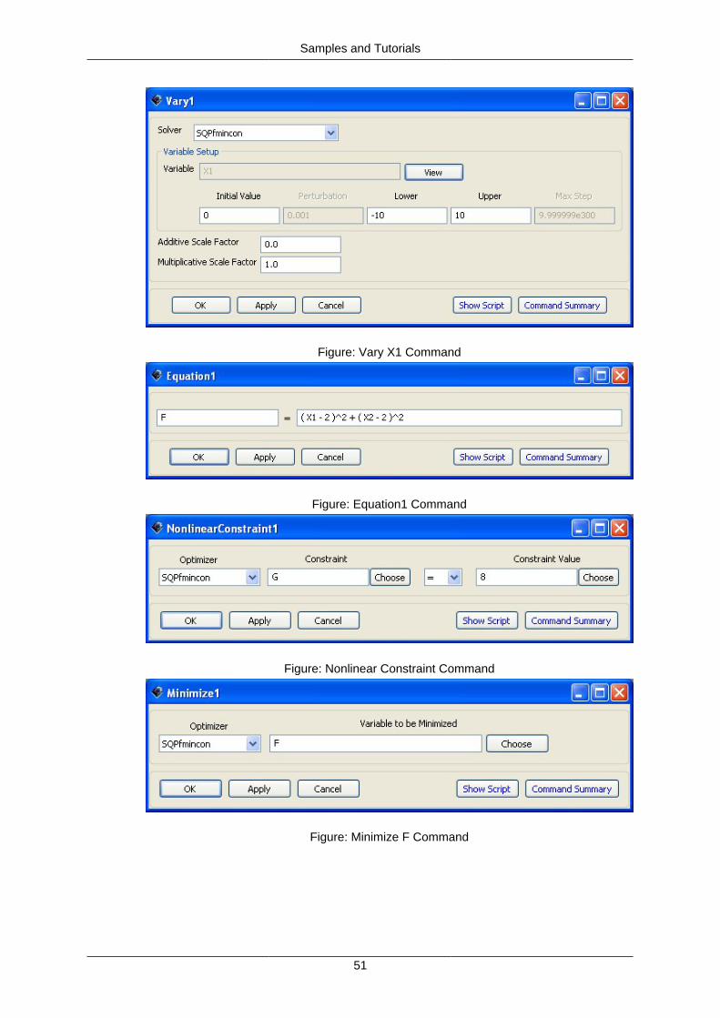
Samples and Tutorials
51
Figure: Vary X1 Command
Figure: Equation1 Command
Figure: Nonlinear Constraint Command
Figure: Minimize F Command
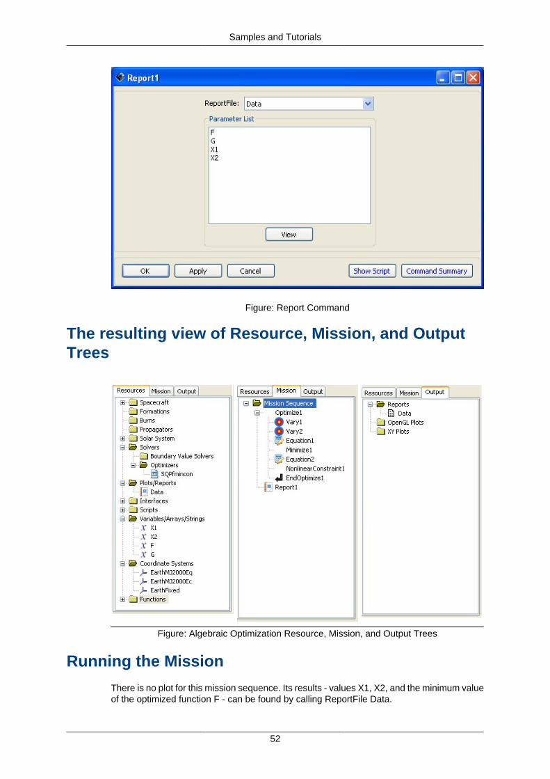
Samples and Tutorials
52
Figure: Report Command
The resulting view of Resource, Mission, and OutputTrees
Figure: Algebraic Optimization Resource, Mission, and Output Trees
Running the Mission
There is no plot for this mission sequence. Its results - values X1, X2, and the minimum valueof the optimized function F - can be found by calling ReportFile Data.
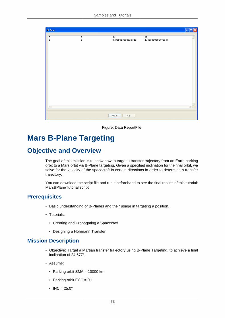
Samples and Tutorials
53
Figure: Data ReportFile
Mars B-Plane Targeting
Objective and OverviewThe goal of this mission is to show how to target a transfer trajectory from an Earth parkingorbit to a Mars orbit via B-Plane targeting. Given a specified inclination for the final orbit, wesolve for the velocity of the spacecraft in certain directions in order to determine a transfertrajectory.
You can download the script file and run it beforehand to see the final results of this tutorial:MarsBPlaneTutorial.script
Prerequisites
• Basic understanding of B-Planes and their usage in targeting a position.
• Tutorials:
• Creating and Propagating a Spacecraft
• Designing a Hohmann Transfer
Mission Description
• Objective: Target a Martian transfer trajectory using B-Plane Targeting, to achieve a finalinclination of 24.677°.
• Assume:
• Parking orbit SMA = 10000 km
• Parking orbit ECC = 0.1
• INC = 25.0°
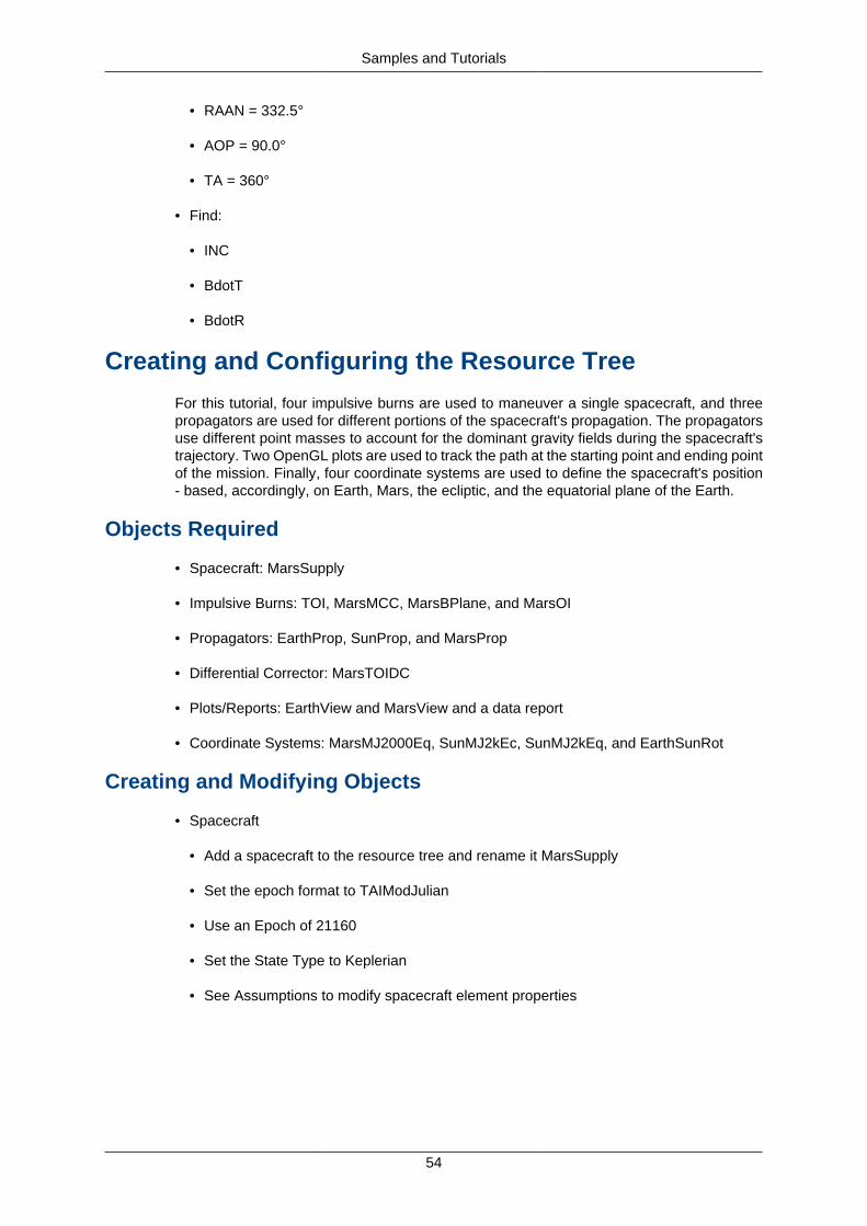
Samples and Tutorials
54
• RAAN = 332.5°
• AOP = 90.0°
• TA = 360°
• Find:
• INC
• BdotT
• BdotR
Creating and Configuring the Resource Tree
For this tutorial, four impulsive burns are used to maneuver a single spacecraft, and threepropagators are used for different portions of the spacecraft's propagation. The propagatorsuse different point masses to account for the dominant gravity fields during the spacecraft'strajectory. Two OpenGL plots are used to track the path at the starting point and ending pointof the mission. Finally, four coordinate systems are used to define the spacecraft's position- based, accordingly, on Earth, Mars, the ecliptic, and the equatorial plane of the Earth.
Objects Required
• Spacecraft: MarsSupply
• Impulsive Burns: TOI, MarsMCC, MarsBPlane, and MarsOI
• Propagators: EarthProp, SunProp, and MarsProp
• Differential Corrector: MarsTOIDC
• Plots/Reports: EarthView and MarsView and a data report
• Coordinate Systems: MarsMJ2000Eq, SunMJ2kEc, SunMJ2kEq, and EarthSunRot
Creating and Modifying Objects
• Spacecraft
• Add a spacecraft to the resource tree and rename it MarsSupply
• Set the epoch format to TAIModJulian
• Use an Epoch of 21160
• Set the State Type to Keplerian
• See Assumptions to modify spacecraft element properties
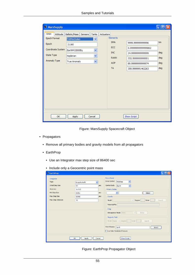
Samples and Tutorials
55
Figure: MarsSupply Spacecraft Object
• Propagators
• Remove all primary bodies and gravity models from all propagators
• EarthProp
• Use an Integrator max step size of 86400 sec
• Include only a Geocentric point mass
Figure: EarthProp Propagator Object
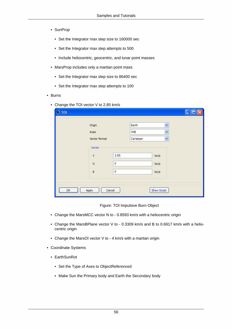
Samples and Tutorials
56
• SunProp
• Set the Integrator max step size to 160000 sec
• Set the Integrator max step attempts to 500
• Include heliocentric, geocentric, and lunar point masses
• MarsProp includes only a martian point mass
• Set the Integrator max step size to 86400 sec
• Set the Integrator max step attempts to 100
• Burns
• Change the TOI vector V to 2.85 km/s
Figure: TOI Impulsive Burn Object
• Change the MarsMCC vector N to - 0.8593 km/s with a heliocentric origin
• Change the MarsBPlane vector V to - 0.3309 km/s and B to 0.6917 km/s with a helio-centric origin
• Change the MarsOI vector V to - 4 km/s with a martian origin
• Coordinate Systems
• EarthSunRot
• Set the Type of Axes to ObjectReferenced
• Make Sun the Primary body and Earth the Secondary body
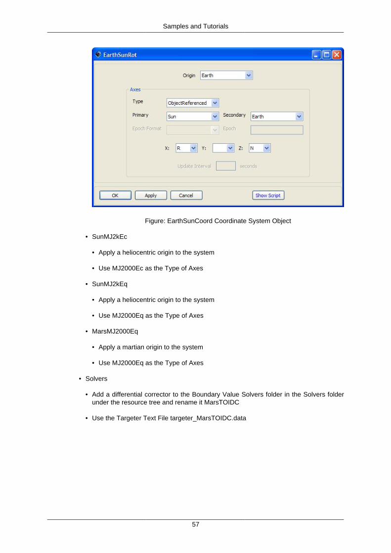
Samples and Tutorials
57
Figure: EarthSunCoord Coordinate System Object
• SunMJ2kEc
• Apply a heliocentric origin to the system
• Use MJ2000Ec as the Type of Axes
• SunMJ2kEq
• Apply a heliocentric origin to the system
• Use MJ2000Eq as the Type of Axes
• MarsMJ2000Eq
• Apply a martian origin to the system
• Use MJ2000Eq as the Type of Axes
• Solvers
• Add a differential corrector to the Boundary Value Solvers folder in the Solvers folderunder the resource tree and rename it MarsTOIDC
• Use the Targeter Text File targeter_MarsTOIDC.data
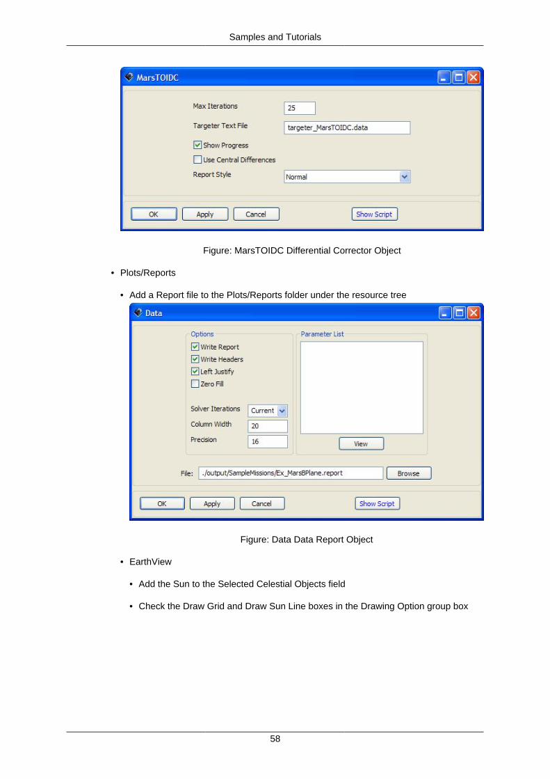
Samples and Tutorials
58
Figure: MarsTOIDC Differential Corrector Object
• Plots/Reports
• Add a Report file to the Plots/Reports folder under the resource tree
Figure: Data Data Report Object
• EarthView
• Add the Sun to the Selected Celestial Objects field
• Check the Draw Grid and Draw Sun Line boxes in the Drawing Option group box
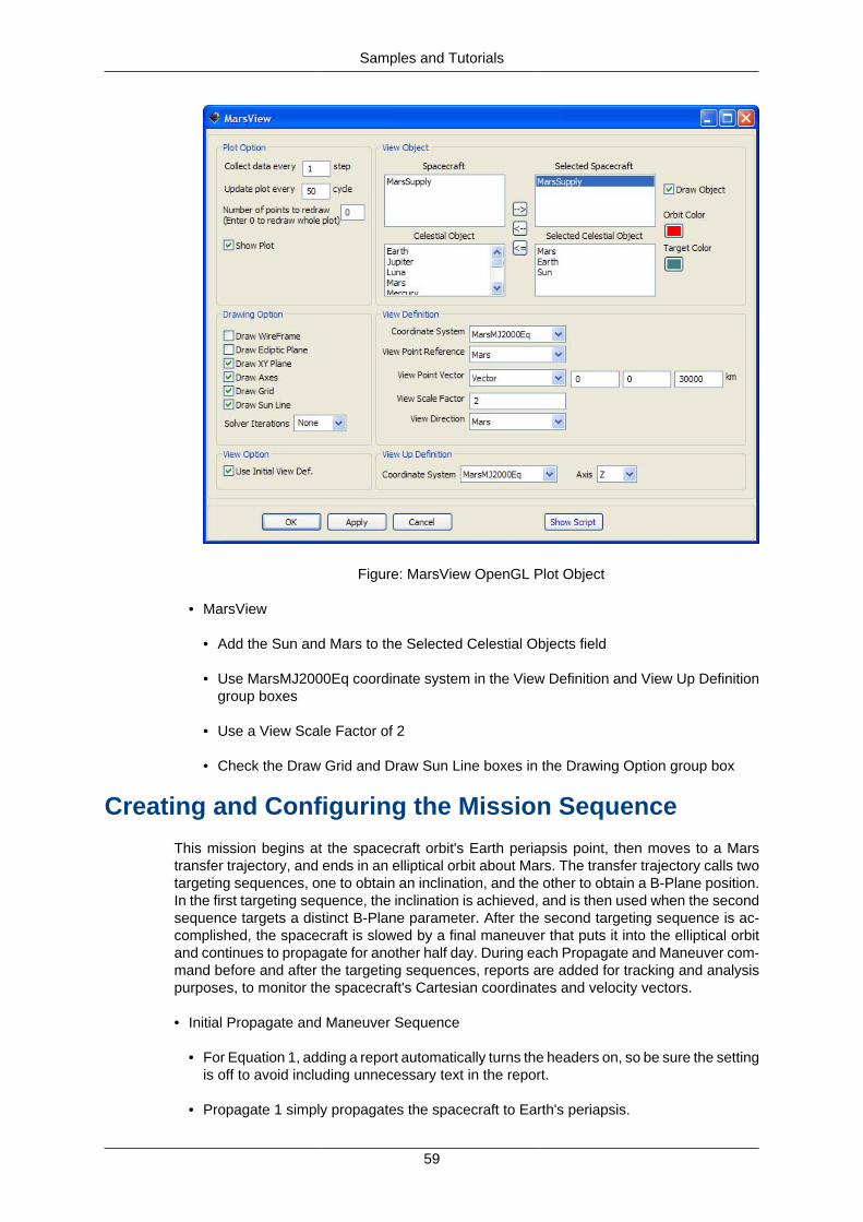
Samples and Tutorials
59
Figure: MarsView OpenGL Plot Object
• MarsView
• Add the Sun and Mars to the Selected Celestial Objects field
• Use MarsMJ2000Eq coordinate system in the View Definition and View Up Definitiongroup boxes
• Use a View Scale Factor of 2
• Check the Draw Grid and Draw Sun Line boxes in the Drawing Option group box
Creating and Configuring the Mission Sequence
This mission begins at the spacecraft orbit's Earth periapsis point, then moves to a Marstransfer trajectory, and ends in an elliptical orbit about Mars. The transfer trajectory calls twotargeting sequences, one to obtain an inclination, and the other to obtain a B-Plane position.In the first targeting sequence, the inclination is achieved, and is then used when the secondsequence targets a distinct B-Plane parameter. After the second targeting sequence is ac-complished, the spacecraft is slowed by a final maneuver that puts it into the elliptical orbitand continues to propagate for another half day. During each Propagate and Maneuver com-mand before and after the targeting sequences, reports are added for tracking and analysispurposes, to monitor the spacecraft's Cartesian coordinates and velocity vectors.
• Initial Propagate and Maneuver Sequence
• For Equation 1, adding a report automatically turns the headers on, so be sure the settingis off to avoid including unnecessary text in the report.
• Propagate 1 simply propagates the spacecraft to Earth's periapsis.
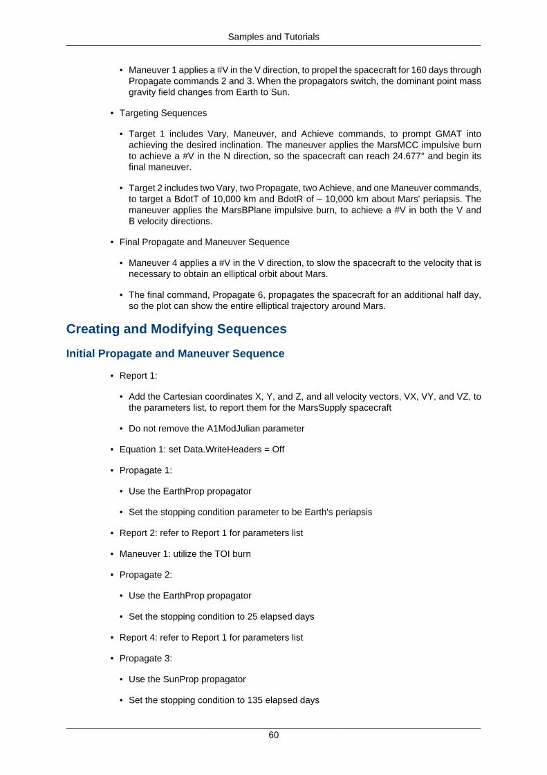
Samples and Tutorials
60
• Maneuver 1 applies a #V in the V direction, to propel the spacecraft for 160 days throughPropagate commands 2 and 3. When the propagators switch, the dominant point massgravity field changes from Earth to Sun.
• Targeting Sequences
• Target 1 includes Vary, Maneuver, and Achieve commands, to prompt GMAT intoachieving the desired inclination. The maneuver applies the MarsMCC impulsive burnto achieve a #V in the N direction, so the spacecraft can reach 24.677° and begin itsfinal maneuver.
• Target 2 includes two Vary, two Propagate, two Achieve, and one Maneuver commands,to target a BdotT of 10,000 km and BdotR of – 10,000 km about Mars' periapsis. Themaneuver applies the MarsBPlane impulsive burn, to achieve a #V in both the V andB velocity directions.
• Final Propagate and Maneuver Sequence
• Maneuver 4 applies a #V in the V direction, to slow the spacecraft to the velocity that isnecessary to obtain an elliptical orbit about Mars.
• The final command, Propagate 6, propagates the spacecraft for an additional half day,so the plot can show the entire elliptical trajectory around Mars.
Creating and Modifying Sequences
Initial Propagate and Maneuver Sequence
• Report 1:
• Add the Cartesian coordinates X, Y, and Z, and all velocity vectors, VX, VY, and VZ, tothe parameters list, to report them for the MarsSupply spacecraft
• Do not remove the A1ModJulian parameter
• Equation 1: set Data.WriteHeaders = Off
• Propagate 1:
• Use the EarthProp propagator
• Set the stopping condition parameter to be Earth's periapsis
• Report 2: refer to Report 1 for parameters list
• Maneuver 1: utilize the TOI burn
• Propagate 2:
• Use the EarthProp propagator
• Set the stopping condition to 25 elapsed days
• Report 4: refer to Report 1 for parameters list
• Propagate 3:
• Use the SunProp propagator
• Set the stopping condition to 135 elapsed days
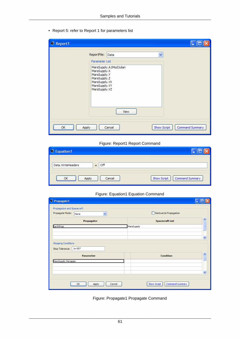
Samples and Tutorials
61
• Report 5: refer to Report 1 for parameters list
Figure: Report1 Report Command
Figure: Equation1 Equation Command
Figure: Propagate1 Propagate Command
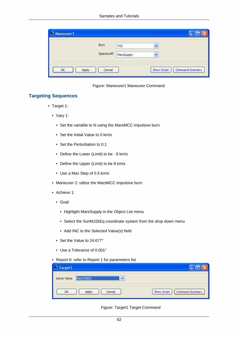
Samples and Tutorials
62
Figure: Maneuver1 Maneuver Command
Targeting Sequences
• Target 1:
• Vary 1:
• Set the variable to N using the MarsMCC impulsive burn
• Set the Initial Value to 0 km/s
• Set the Perturbation to 0.1
• Define the Lower (Limit) to be - 8 km/s
• Define the Upper (Limit) to be 8 km/s
• Use a Max Step of 0.5 km/s
• Maneuver 2: utilize the MarsMCC impulsive burn
• Achieve 1:
• Goal:
• Highlight MarsSupply in the Object List menu
• Select the SunMJ2kEq coordinate system from the drop down menu
• Add INC to the Selected Value(s) field
• Set the Value to 24.677°
• Use a Tolerance of 0.001°
• Report 6: refer to Report 1 for parameters list
Figure: Target1 Target Command
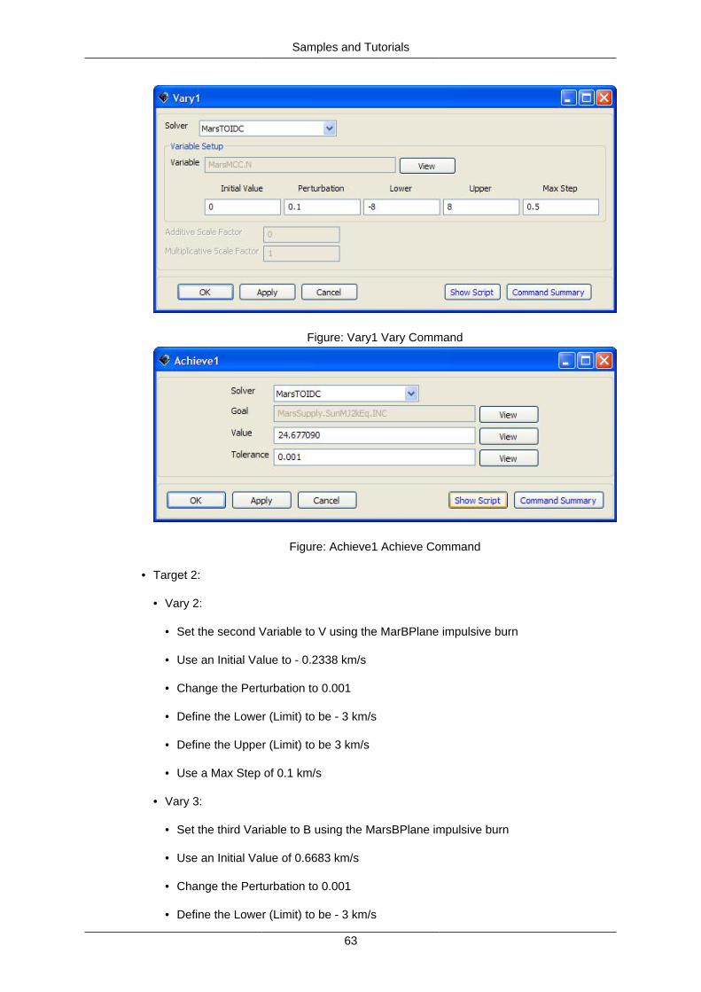
Samples and Tutorials
63
Figure: Vary1 Vary Command
Figure: Achieve1 Achieve Command
• Target 2:
• Vary 2:
• Set the second Variable to V using the MarBPlane impulsive burn
• Use an Initial Value to - 0.2338 km/s
• Change the Perturbation to 0.001
• Define the Lower (Limit) to be - 3 km/s
• Define the Upper (Limit) to be 3 km/s
• Use a Max Step of 0.1 km/s
• Vary 3:
• Set the third Variable to B using the MarsBPlane impulsive burn
• Use an Initial Value of 0.6683 km/s
• Change the Perturbation to 0.001
• Define the Lower (Limit) to be - 3 km/s
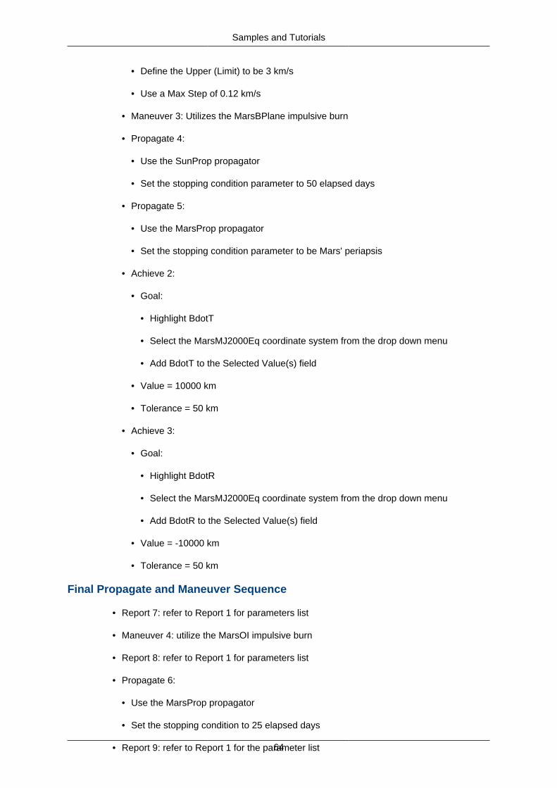
Samples and Tutorials
64
• Define the Upper (Limit) to be 3 km/s
• Use a Max Step of 0.12 km/s
• Maneuver 3: Utilizes the MarsBPlane impulsive burn
• Propagate 4:
• Use the SunProp propagator
• Set the stopping condition parameter to 50 elapsed days
• Propagate 5:
• Use the MarsProp propagator
• Set the stopping condition parameter to be Mars' periapsis
• Achieve 2:
• Goal:
• Highlight BdotT
• Select the MarsMJ2000Eq coordinate system from the drop down menu
• Add BdotT to the Selected Value(s) field
• Value = 10000 km
• Tolerance = 50 km
• Achieve 3:
• Goal:
• Highlight BdotR
• Select the MarsMJ2000Eq coordinate system from the drop down menu
• Add BdotR to the Selected Value(s) field
• Value = -10000 km
• Tolerance = 50 km
Final Propagate and Maneuver Sequence
• Report 7: refer to Report 1 for parameters list
• Maneuver 4: utilize the MarsOI impulsive burn
• Report 8: refer to Report 1 for parameters list
• Propagate 6:
• Use the MarsProp propagator
• Set the stopping condition to 25 elapsed days
• Report 9: refer to Report 1 for the parameter list
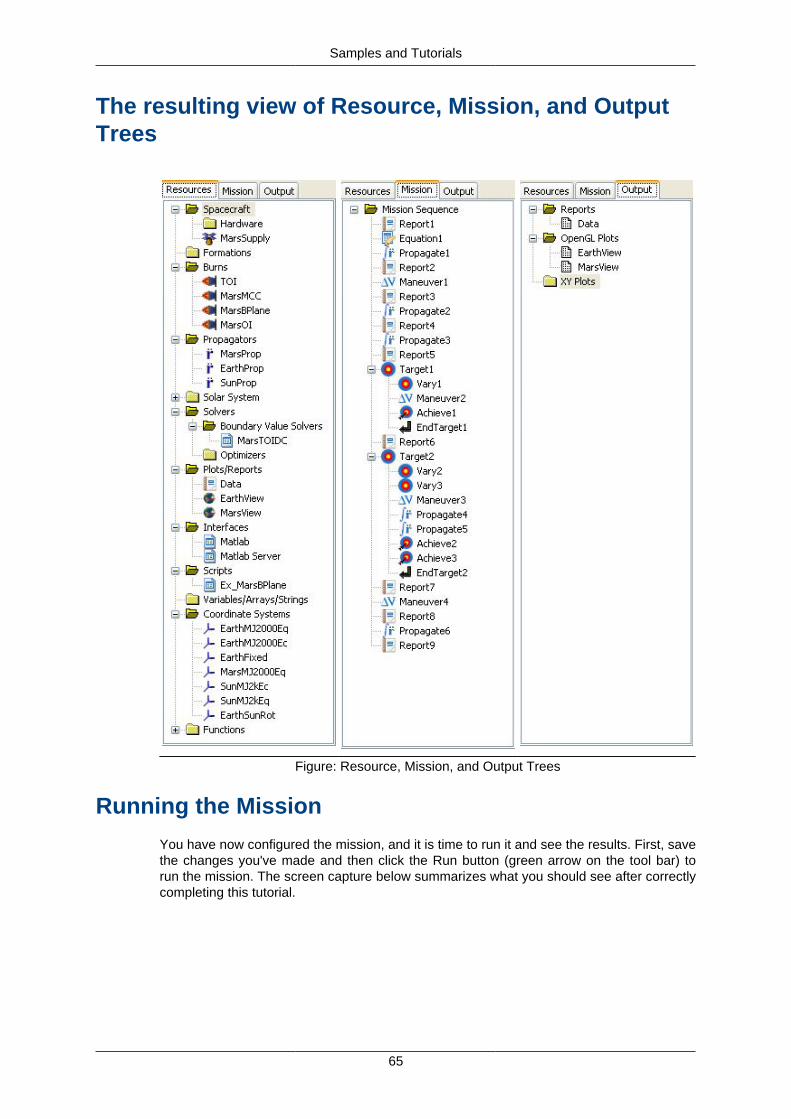
Samples and Tutorials
65
The resulting view of Resource, Mission, and OutputTrees
Figure: Resource, Mission, and Output Trees
Running the Mission
You have now configured the mission, and it is time to run it and see the results. First, savethe changes you've made and then click the Run button (green arrow on the tool bar) torun the mission. The screen capture below summarizes what you should see after correctlycompleting this tutorial.
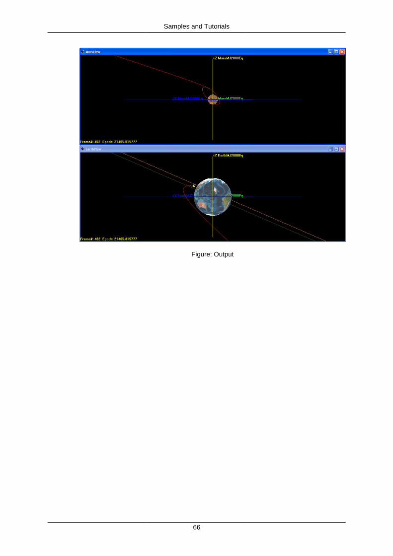
Samples and Tutorials
66
Figure: Output

Reference Guide
68
Table of ContentsI. Resources ............................................................................................................ 69
Array ................................................................................................................ 70Barycenter ....................................................................................................... 71CelestialBodies ................................................................................................. 72CoordinateSystem ............................................................................................ 75DifferentialCorrector .......................................................................................... 76EphemerisFile .................................................................................................. 79EphemerisPropagator ....................................................................................... 80FiniteBurn ........................................................................................................ 81Formation ......................................................................................................... 83FuelTank .......................................................................................................... 84GroundStation .................................................................................................. 86ImpulsiveBurn .................................................................................................. 87LibrationPoint ................................................................................................... 89MATLABFunction .............................................................................................. 90OpenGLPlot ..................................................................................................... 91Propagator ....................................................................................................... 96ReportFile ...................................................................................................... 102SolarSystem ................................................................................................... 105Spacecraft ...................................................................................................... 107SQP ............................................................................................................... 112String ............................................................................................................. 115Thruster ......................................................................................................... 116Variable ......................................................................................................... 121VF13adOptimizer ............................................................................................ 122XYPlot ........................................................................................................... 123
II. Commands ......................................................................................................... 125Achieve .......................................................................................................... 126BeginFiniteBurn .............................................................................................. 127BeginMissionSequence ................................................................................... 128CallFunction ................................................................................................... 129Else ............................................................................................................... 131EndFiniteBurn ................................................................................................. 132Equation ......................................................................................................... 133For ................................................................................................................. 134If .................................................................................................................... 136Maneuver ....................................................................................................... 138Minimize ......................................................................................................... 139NonLinearConstraint ....................................................................................... 141Optimize ......................................................................................................... 143PenUp ........................................................................................................... 145PenDown ....................................................................................................... 146Propagate ...................................................................................................... 147Report ............................................................................................................ 150Save .............................................................................................................. 151ScriptEvent ..................................................................................................... 152Stop ............................................................................................................... 153Target ............................................................................................................ 154Toggle ........................................................................................................... 156Vary ............................................................................................................... 158While ............................................................................................................. 161

69
Resources
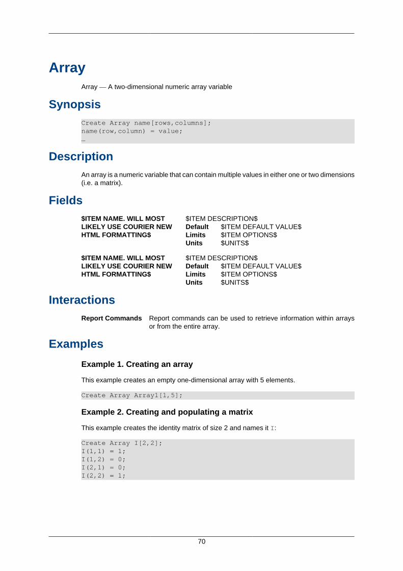
70
ArrayArray — A two-dimensional numeric array variable
SynopsisCreate Array name[rows,columns];name(row,column) = value;…
DescriptionAn array is a numeric variable that can contain multiple values in either one or two dimensions(i.e. a matrix).
Fields$ITEM NAME. WILL MOSTLIKELY USE COURIER NEWHTML FORMATTING$
$ITEM DESCRIPTION$Default $ITEM DEFAULT VALUE$Limits $ITEM OPTIONS$Units $UNITS$
$ITEM NAME. WILL MOSTLIKELY USE COURIER NEWHTML FORMATTING$
$ITEM DESCRIPTION$Default $ITEM DEFAULT VALUE$Limits $ITEM OPTIONS$Units $UNITS$
InteractionsReport Commands Report commands can be used to retrieve information within arrays
or from the entire array.
Examples
Example 1. Creating an array
This example creates an empty one-dimensional array with 5 elements.
Create Array Array1[1,5];
Example 2. Creating and populating a matrix
This example creates the identity matrix of size 2 and names it I:
Create Array I[2,2];I(1,1) = 1;I(1,2) = 0;I(2,1) = 0;I(2,2) = 1;
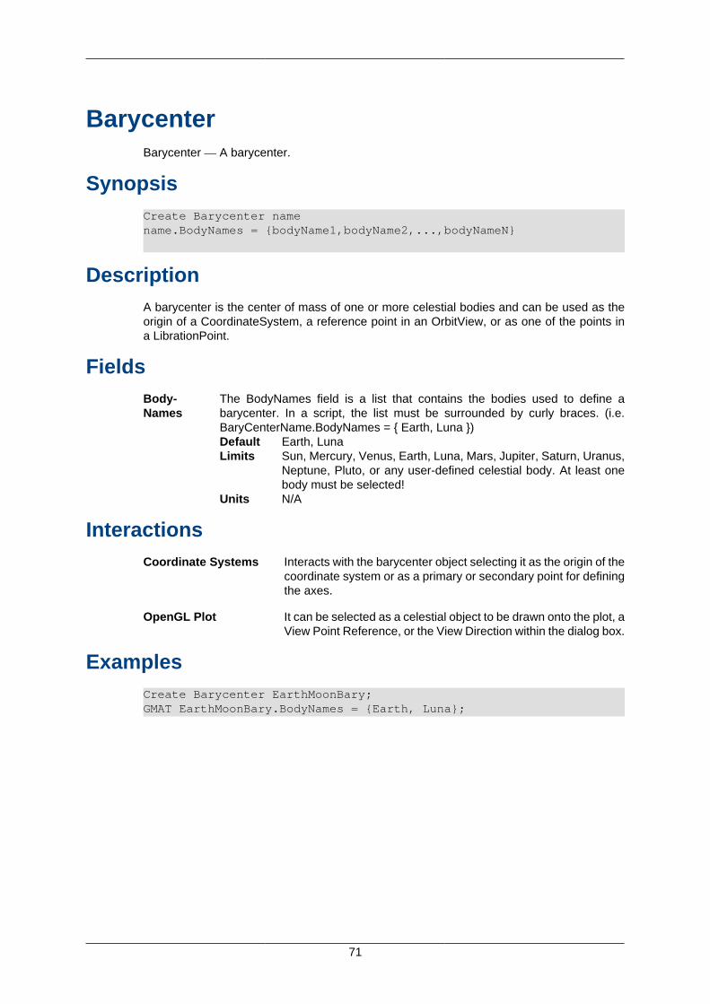
71
BarycenterBarycenter — A barycenter.
SynopsisCreate Barycenter namename.BodyNames = {bodyName1,bodyName2,...,bodyNameN}
DescriptionA barycenter is the center of mass of one or more celestial bodies and can be used as theorigin of a CoordinateSystem, a reference point in an OrbitView, or as one of the points ina LibrationPoint.
FieldsBody-Names
The BodyNames field is a list that contains the bodies used to define abarycenter. In a script, the list must be surrounded by curly braces. (i.e.BaryCenterName.BodyNames = { Earth, Luna }) Default Earth, LunaLimits Sun, Mercury, Venus, Earth, Luna, Mars, Jupiter, Saturn, Uranus,
Neptune, Pluto, or any user-defined celestial body. At least onebody must be selected!
Units N/A
InteractionsCoordinate Systems Interacts with the barycenter object selecting it as the origin of the
coordinate system or as a primary or secondary point for definingthe axes.
OpenGL Plot It can be selected as a celestial object to be drawn onto the plot, aView Point Reference, or the View Direction within the dialog box.
ExamplesCreate Barycenter EarthMoonBary;GMAT EarthMoonBary.BodyNames = {Earth, Luna};
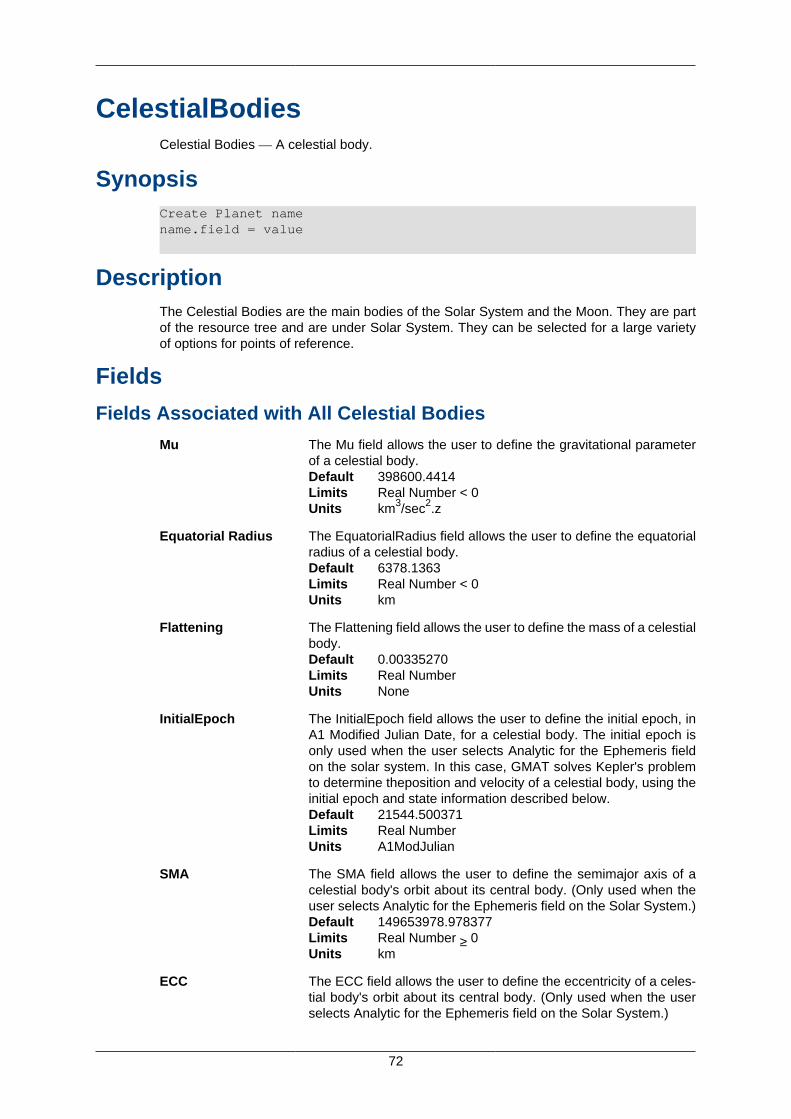
72
CelestialBodiesCelestial Bodies — A celestial body.
SynopsisCreate Planet namename.field = value
DescriptionThe Celestial Bodies are the main bodies of the Solar System and the Moon. They are partof the resource tree and are under Solar System. They can be selected for a large varietyof options for points of reference.
Fields
Fields Associated with All Celestial Bodies
Mu The Mu field allows the user to define the gravitational parameterof a celestial body.Default 398600.4414Limits Real Number < 0Units km3/sec2.z
Equatorial Radius The EquatorialRadius field allows the user to define the equatorialradius of a celestial body.Default 6378.1363Limits Real Number < 0Units km
Flattening The Flattening field allows the user to define the mass of a celestialbody.Default 0.00335270Limits Real NumberUnits None
InitialEpoch The InitialEpoch field allows the user to define the initial epoch, inA1 Modified Julian Date, for a celestial body. The initial epoch isonly used when the user selects Analytic for the Ephemeris fieldon the solar system. In this case, GMAT solves Kepler's problemto determine theposition and velocity of a celestial body, using theinitial epoch and state information described below.Default 21544.500371Limits Real NumberUnits A1ModJulian
SMA The SMA field allows the user to define the semimajor axis of acelestial body's orbit about its central body. (Only used when theuser selects Analytic for the Ephemeris field on the Solar System.)Default 149653978.978377Limits Real Number ≥ 0Units km
ECC The ECC field allows the user to define the eccentricity of a celes-tial body's orbit about its central body. (Only used when the userselects Analytic for the Ephemeris field on the Solar System.)
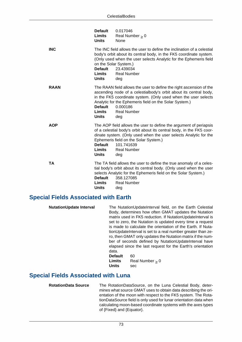
CelestialBodies
73
Default 0.017046Limits Real Number ≥ 0Units None
INC The INC field allows the user to define the inclination of a celestialbody's orbit about its central body, in the FK5 coordinate system.(Only used when the user selects Analytic for the Ephemeris fieldon the Solar System.)Default 23.439034Limits Real NumberUnits deg
RAAN The RAAN field allows the user to define the right ascension of theascending node of a celestialbody's orbit about its central body,in the FK5 coordinate system. (Only used when the user selectsAnalytic for the Ephemeris field on the Solar System.)Default 0.000186Limits Real NumberUnits deg
AOP The AOP field allows the user to define the argument of periapsisof a celestial body's orbit about its central body, in the FK5 coor-dinate system. (Only used when the user selects Analytic for theEphemeris field on the Solar System.)Default 101.741639Limits Real NumberUnits deg
TA The TA field allows the user to define the true anomaly of a celes-tial body's orbit about its central body. (Only used when the userselects Analytic for the Ephemeris field on the Solar System.)Default 358.127085Limits Real NumberUnits deg
Special Fields Associated with Earth
NutationUpdate Interval The NutationUpdateInterval field, on the Earth CelestialBody, determines how often GMAT updates the Nutationmatrix used in FK5 reduction. If NutationUpdateInterval isset to zero, the Nutation is updated every time a requestis made to calculate the orientation of the Earth. If Nuta-tionUpdateInterval is set to a real number greater than ze-ro, then GMAT only updates the Nutation matrix if the num-ber of seconds defined by NutationUpdateInterval haveelapsed since the last request for the Earth's orientationdata.Default 60Limits Real Number ≥ 0Units sec
Special Fields Associated with Luna
RotationData Source The RotationDataSource, on the Luna Celestial Body, deter-mines what source GMAT uses to obtain data describing the ori-entation of the moon with respect to the FK5 system. The Rota-tionDataSource field is only used for lunar orientation data whencalculating moon-based coordinate systems with the axes typesof {Fixed} and {Equator}.
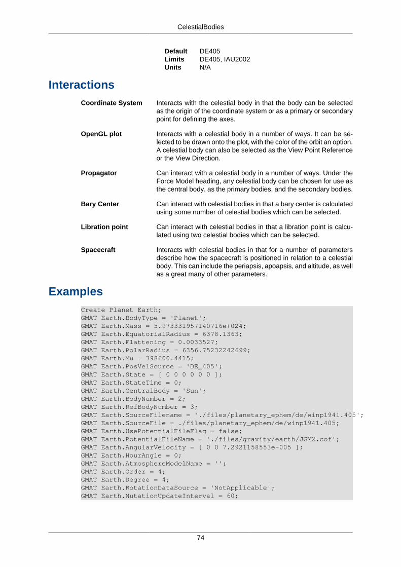
CelestialBodies
74
Default DE405Limits DE405, IAU2002Units N/A
InteractionsCoordinate System Interacts with the celestial body in that the body can be selected
as the origin of the coordinate system or as a primary or secondarypoint for defining the axes.
OpenGL plot Interacts with a celestial body in a number of ways. It can be se-lected to be drawn onto the plot, with the color of the orbit an option.A celestial body can also be selected as the View Point Referenceor the View Direction.
Propagator Can interact with a celestial body in a number of ways. Under theForce Model heading, any celestial body can be chosen for use asthe central body, as the primary bodies, and the secondary bodies.
Bary Center Can interact with celestial bodies in that a bary center is calculatedusing some number of celestial bodies which can be selected.
Libration point Can interact with celestial bodies in that a libration point is calcu-lated using two celestial bodies which can be selected.
Spacecraft Interacts with celestial bodies in that for a number of parametersdescribe how the spacecraft is positioned in relation to a celestialbody. This can include the periapsis, apoapsis, and altitude, as wellas a great many of other parameters.
ExamplesCreate Planet Earth;GMAT Earth.BodyType = 'Planet';GMAT Earth.Mass = 5.973331957140716e+024;GMAT Earth.EquatorialRadius = 6378.1363;GMAT Earth.Flattening = 0.0033527;GMAT Earth.PolarRadius = 6356.75232242699;GMAT Earth.Mu = 398600.4415;GMAT Earth.PosVelSource = 'DE_405';GMAT Earth.State = [ 0 0 0 0 0 0 ];GMAT Earth.StateTime = 0;GMAT Earth.CentralBody = 'Sun';GMAT Earth.BodyNumber = 2;GMAT Earth.RefBodyNumber = 3;GMAT Earth.SourceFilename = './files/planetary_ephem/de/winp1941.405';GMAT Earth.SourceFile = ./files/planetary_ephem/de/winp1941.405;GMAT Earth.UsePotentialFileFlag = false;GMAT Earth.PotentialFileName = './files/gravity/earth/JGM2.cof';GMAT Earth.AngularVelocity = [ 0 0 7.2921158553e-005 ];GMAT Earth.HourAngle = 0;GMAT Earth.AtmosphereModelName = '';GMAT Earth.Order = 4;GMAT Earth.Degree = 4;GMAT Earth.RotationDataSource = 'NotApplicable';GMAT Earth.NutationUpdateInterval = 60;
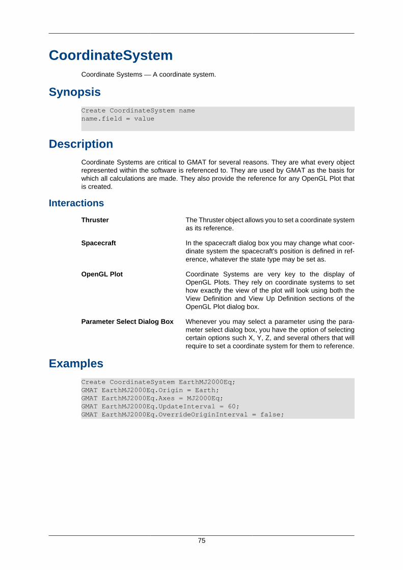
75
CoordinateSystemCoordinate Systems — A coordinate system.
SynopsisCreate CoordinateSystem namename.field = value
DescriptionCoordinate Systems are critical to GMAT for several reasons. They are what every objectrepresented within the software is referenced to. They are used by GMAT as the basis forwhich all calculations are made. They also provide the reference for any OpenGL Plot thatis created.
Interactions
Thruster The Thruster object allows you to set a coordinate systemas its reference.
Spacecraft In the spacecraft dialog box you may change what coor-dinate system the spacecraft's position is defined in ref-erence, whatever the state type may be set as.
OpenGL Plot Coordinate Systems are very key to the display ofOpenGL Plots. They rely on coordinate systems to sethow exactly the view of the plot will look using both theView Definition and View Up Definition sections of theOpenGL Plot dialog box.
Parameter Select Dialog Box Whenever you may select a parameter using the para-meter select dialog box, you have the option of selectingcertain options such X, Y, Z, and several others that willrequire to set a coordinate system for them to reference.
ExamplesCreate CoordinateSystem EarthMJ2000Eq;GMAT EarthMJ2000Eq.Origin = Earth;GMAT EarthMJ2000Eq.Axes = MJ2000Eq;GMAT EarthMJ2000Eq.UpdateInterval = 60;GMAT EarthMJ2000Eq.OverrideOriginInterval = false;
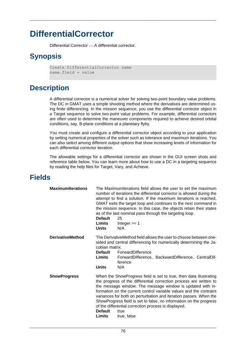
76
DifferentialCorrectorDifferential Corrector — A differential corrector.
SynopsisCreate DifferentialCorrector namename.field = value
DescriptionA differential corrector is a numerical solver for solving two-point boundary value problems.The DC in GMAT uses a simple shooting method where the derivatives are determined us-ing finite differencing. In the mission sequence, you use the differential corrector object ina Target sequence to solve two-point value problems. For example, differential correctorsare often used to determine the maneuver components required to achieve desired orbitalconditions, say, B-plane conditions at a planetary flyby.
You must create and configure a differential corrector object according to your applicationby setting numerical properties of the solver such as tolerance and maximum iterations. Youcan also select among different output options that show increasing levels of information foreach differential corrector iteration.
The allowable settings for a differential corrector are shown in the GUI screen shots andreference table below. You can learn more about how to use a DC in a targeting sequenceby reading the help files for Target, Vary, and Achieve.
FieldsMaximumIterations The MaximumIterations field allows the user to set the maximum
number of iterations the differential corrector is allowed during theattempt to find a solution. If the maximum iterations is reached,GMAT exits the target loop and continues to the next command inthe mission sequence. In this case, the objects retain their statesas of the last nominal pass through the targeting loop.Default 25Limits Integer >= 1Units N/A
DerivativeMethod The DerivativeMethod field allows the user to choose between one-sided and central differencing for numerically determining the Ja-cobian matrix.Default ForwardDifferenceLimits ForwardDifference, BackwardDifference, CentralDif-
ferenceUnits N/A
ShowProgress When the ShowProgress field is set to true, then data illustratingthe progress of the differential correction process are written tothe message window. The message window is updated with in-formation on the current control variable values and the contraintvariances for both on perturbation and iteration passes. When theShowProgress field is set to false, no information on the progressof the differential correction process is displayed.Default trueLimits true, false
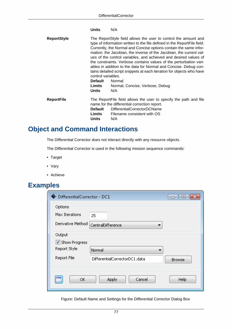
DifferentialCorrector
77
Units N/A
ReportStyle The ReportStyle field allows the user to control the amount andtype of information written to the file defined in the ReportFile field.Currently, the Normal and Concise options contain the same infor-mation: the Jacobian, the inverse of the Jacobian, the current val-ues of the control variables, and achieved and desired values ofthe constraints. Verbose contains values of the perturbation vari-ables in addition to the data for Normal and Concise. Debug con-tains detailed script snippets at each iteration for objects who havecontrol variables.Default NormalLimits Normal, Concise, Verbose, DebugUnits N/A
ReportFile The ReportFile field allows the user to specify the path and filename for the differential correction report.Default DifferentialCorrectorDCNameLimits Filename consistent with OSUnits N/A
Object and Command InteractionsThe Differential Corrector does not interact directly with any resource objects.
The Differential Corrector is used in the following mission sequence commands:
• Target
• Vary
• Achieve
Examples
Figure: Default Name and Settings for the Differential Corrector Dialog Box
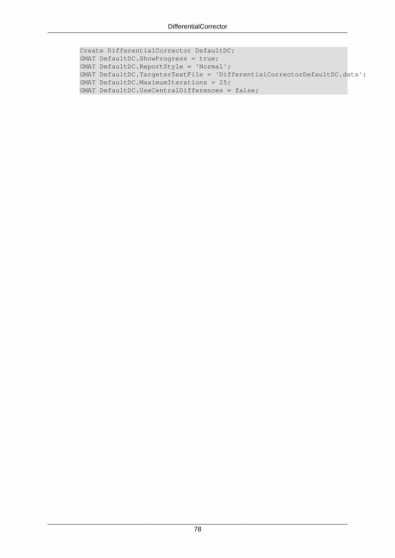
DifferentialCorrector
78
Create DifferentialCorrector DefaultDC;GMAT DefaultDC.ShowProgress = true;GMAT DefaultDC.ReportStyle = 'Normal';GMAT DefaultDC.TargeterTextFile = 'DifferentialCorrectorDefaultDC.data';GMAT DefaultDC.MaximumIterations = 25;GMAT DefaultDC.UseCentralDifferences = false;
79
EphemerisFileEphemerisFile — An ephemeris file.
Synopsis Under Construction.
DescriptionUnder Construction.
FieldsField Name Description....
Type Fill This In.Default Fill This In.Limits Fill This In.Units Fill This In.
Examples
Example 3. Example Script
%
80
EphemerisPropagatorEphemerisPropagator — Under Construction.
Synopsis Under Construction.
DescriptionUnder Construction.
FieldsField Name Description....
Type Fill This In.Default Fill This In.Limits Fill This In.Units Fill This In.
Examples
Example 4. Example Script
%
81
FiniteBurnFinite Burn — A finite burn.
SynopsisCreate FiniteBurn namename.field = value
DescriptionThe Finite Burn object is used when a continuous propulsion is desired. Impulsive burnshappen instantaneously and through a Maneuver command, while finite burns occur until theEnd Finite Burn command is reached in the mission sequence and are typically coupled withPropagate commands.
FieldsOrigin Together the Origin and Axes fields describe the coordinate system in
which a maneuver is applied. The Origin field determines the origin ofthe maneuver coordinate system. The ability to define the coordinatesystem locally avoids having to create many coordinate systems, as-sociated with specific spacecraft, in order to perform finite maneuversfor multiple spacecraft.Default EarthLimits Any celestial body, libration point, or barycenterUnits N/A
Axes The Axes field, together with the Origin field, describe the coordinatesystem in which a finite maneuver is applied. If VNB is chosen for Ax-es, a local coordinate system is created such that the x-axis pointsin the velocity direction of the spacecraft, with respect to the point de-fined by Origin, the y-axis points in the normal direction of the space-craft with respect to Origin, and the z-axis completes the right-handedset.Default VNBLimits VNB, MJ2000EqUnits N/A
Thrusters The Thrusters field allows the selection of which thrusters to usewhen applying a finite maneuver. The user can select more than onethruster, from the list of thrusters previously created, by including allthrusters in curly braces. An example is MyFiniteBurn.Thrusters =Thruster1,Thruster2,Thruster3.Default No DefaultLimits Any thruster created by userUnits N/A
BurnScaleFactor The BurnScaleFactor is used to scale the total acceleration beforeadding the acceleration due to a finite burn into the sum of the accel-erations of a spacecraft. The scaling is performed by taking the sum ofthe accelerations applied by all thrusters specified under the Thrustersfield, and multiplying the total thrust by BurnScaleFactor.Default 1.0Limits Real NumberUnits N/A
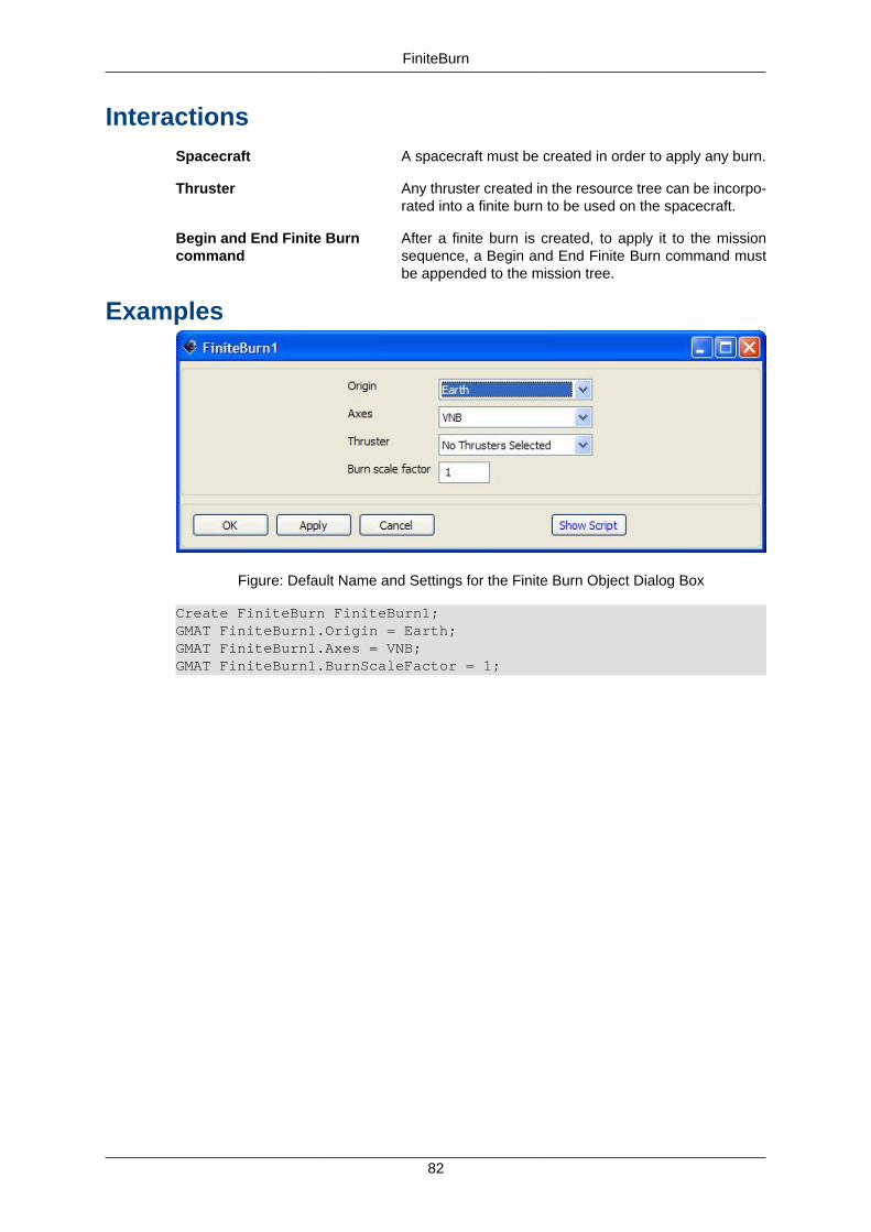
FiniteBurn
82
InteractionsSpacecraft A spacecraft must be created in order to apply any burn.
Thruster Any thruster created in the resource tree can be incorpo-rated into a finite burn to be used on the spacecraft.
Begin and End Finite Burncommand
After a finite burn is created, to apply it to the missionsequence, a Begin and End Finite Burn command mustbe appended to the mission tree.
Examples
Figure: Default Name and Settings for the Finite Burn Object Dialog Box
Create FiniteBurn FiniteBurn1;GMAT FiniteBurn1.Origin = Earth;GMAT FiniteBurn1.Axes = VNB;GMAT FiniteBurn1.BurnScaleFactor = 1;
83
FormationFormation — An ephemeris file.
Synopsis Under Construction.
DescriptionUnder Construction.
FieldsField Name Description....
Type Fill This In.Default Fill This In.Limits Fill This In.Units Fill This In.
Examples
Example 5. Example Script
%
84
FuelTankFuelTank — A fuel tank.
SynopsisCreate FuelTank namename.field = value
DescriptionA FuelTank is a thermodynamc model of a tank and is required for finite burn modelling orfor implusive burns that use mass depletion. The thermodynamic properties of the tank aremodelled using the ideal gas law and assume that there is no energy transfer into or out of thetank as fuel is depleted. To use a FuelTank, you must first create the tank, and then attachit to the desired spacecraft and associate it with a thruster as shown in the examples below.
FieldsPressure The pressure in the tank.
Type Real NumberDefault 1500Limits Pressure > 0Units kPa.
Temperature The temperature of the fuel and ullage in the tank. GMAT currently assumesullage and fuel are always at the same temperature.Type Real NumberDefault 20Limits Temperature > -273.15Units C.
FuelMass The FuelMass field is the mass of fuel in the tank.
Caution
By default, GMAT will not allow the fuel mass to be negative.However, occasionally in iterative processes such as target-ing, a solver will try values of a maneuver parameter that re-sult in total fuel depletion. Using the default tank settings thiswill throw an excpeption stopping the run unless you set theAllowNegativeFuelMass flag to true.
Type Real NumberDefault 756Limits FuelMass > 0Units kg.
ReferenceTemperature The temperature of the tank when fuel was loaded.Type Real NumberDefault 20Options ReferenceTemperature >=; 0Units C.
Volume The volume of the tank. GMAT checks to ensure that the vol-ume of the tank is larger than the volume of fuel loaded in the
FuelTank
85
tank and throws an exception in the case that the fuel volumeis larger than the tank volume.Type Real NumberDefault 0.75Options Real Number > 0 such that fuel volume is < tank
volume.Units m3.
FuelDensity The density of the fuel.Type Real NumerDefault 1260Limits Real Number > 0Units kg/m3.
PressureModel The pressure model describes how pressure in the tankchanges as fuel is depleted.Type EnumerationDefault PressureRegulatedLimits PressureRegulated, BlowDownUnits N/A
AllowNegativeFuelMass This field allows the fuel tank to have negagive fuel masswhich can be useful in optimization and targeting sequencesbefore convergences has occurred.Default falseOptions true, false.Units N/A
Examples
Example 6. Creating a default FuelTank and attaching it to a Spacecraft
% Create the Fuel Tank ObjectCreate FuelTank aTank;aTank.AllowNegativeFuelMass = false;aTank.FuelMass = 756;aTank.Pressure = 1500;aTank.Temperature = 20;aTank.RefTemperature = 20;aTank.Volume = 0.75;aTank.FuelDensity = 1260;aTank.PressureModel = PressureRegulated;
% Create a Thruster and assign it a FuelTankCreate Thruster aThruster;aThruster.Tank = {aTank};
% Add the FuelTank and Thruster to a SpacecraftCreate Spacecraft aSpacecraftaSpacecraft.Tanks = {aTank};aSpacecraft.Thrusters = {aThruster};

86
GroundStationGroundStation — Under Construction.
Synopsis Under Construction.
DescriptionUnder Construction.
FieldsField Name Description....
Type Fill This In.Default Fill This In.Limits Fill This In.Units Fill This In.
Examples
Example 7. Example Script
%
87
ImpulsiveBurnImpulsive Burn — A impulsive burn.
SynopsisCreate ImpulsiveBurn namename.field = value
DescriptionThe impulsive burn object in GMAT allows the spacecraft to undergo an instantaneous #Vin up to three dimensions as opposed to a finite burn which is not instantaneous. The usercan configure the burn by defining its origin, type of axes, vector format, and magnitude ofthe vectors. Depending on the mission, it will be simpler to use one axes or vector formatover the other.
Possible Coupling with Other Objects
Spacecraft Must be created in order to apply any burn. The purpose of the im-pulsive burn is to instantaneously propel the spacecraft to either tar-get or optimize a goal during its mission.
Maneuver com-mand
Must be created to call the burn into the mission sequence becausewithout a maneuver, the spacecraft simply propagates around aspecified trajectory. If there are several burns that exist, in the Ma-neuver dialog box the user can choose which burn to utilize for thatpart of the mission sequence. In addition, a Propagate commandmust follow the maneuver to allow the trajectory to unfold after a burnhas been applied.
Vary command Required a burn to be specified in the Variable Setup group box. Thepurpose of the Vary command is to apply a burn in order to changea parameter of the spacecraft's trajectory.
FieldsOrigin Together the Origin and Axes fields describe the coordinate system in
which a maneuver is applied. The Origin field determines the origin ofthe maneuver coordinatesystem. The ability to define the coordinate sys-tem locally avoids having to create many coordinate systems, associatedwith specific spacecraft, in order to perform finite maneuvers for multiplespacecraft.Default EarthLimits Any celestial bodyUnits N/A
Axes The Axes field, together with the Origin field, describethe coordinate sys-tem in which an impulsive maneuver is applied. If VNB is chosen for Axes,a local coordinate system is created such that the x-axis points in the ve-locity direction of thespacecraft, with respect to the point defined by Ori-gin, the y-axis points in the normal direction of the spacecraft with respectto Origin, and the z-axis completes the right-handed set.Default VNBLimits VNB, MJ2000EqUnits N/A
ImpulsiveBurn
88
VectorFormat The VectorFormat field allows the user to define the format of the maneu-ver vector.Default CartesianLimits CartesianUnits N/A
Element1 The Element1 field allows the user to define the first element of the impul-sive maneuver vector. Element1 is X if VectorFormat is Cartesian.Default 0Limits Real NumberUnits km/sec
Element2 The Element2 field allows the user to define the second element of theimpulsive maneuver vector. Element2 is Y if VectorFormat is Cartesian.Default 0Limits Real NumberUnits km/sec
Element3 The Element3 field allows the user to define the third element of the im-pulsive maneuver vector. Element3 is Z if VectorFormat is Cartesian.Default 0Limits Real NumberUnits km/sec
ExamplesCreate ImpulsiveBurn ImpulsiveBurn1;GMAT ImpulsiveBurn1.Origin = Earth;GMAT ImpulsiveBurn1.Axes = VNB;GMAT ImpulsiveBurn1.VectorFormat = Cartesian;GMAT ImpulsiveBurn1.Element1 = 0;GMAT ImpulsiveBurn1.Element2 = 0;GMAT ImpulsiveBurn1.Element3 = 0;
89
LibrationPointLibration Point — A libration point.
SynopsisCreate LibrationPoint namename.field = value
DescriptionA Libration point, also called a Lagrange point, is a point of equilibrium in the restricted three-body problem.
FieldsPrimary The Primary field allows you to define the body treated as the primary in the
calculation of the libration point location. (See Math. Spec for more details).Default SunLimits Sun, Mercury, Venus, Earth, Luna, Mars, Jupiter, Saturn, Uranus,
Neptune, Pluto, or any Barycenter. ( The Primary and Secondarybodies cannot be the same )
Units N/A
Secondary The Secondary field allows you to define the body treated as the secondaryin the calculation of the libration point location.Default EarthLimits Sun, Mercury, Venus, Earth, Luna, Mars, Jupiter, Saturn, Uranus,
Neptune, Pluto, or any Barycenter. ( The Primary and Secondarybodies cannot be the same )
Units N/A
Point The Point field specifies which libration point the object corresponds to.Default L1Limits L1, L2, L3, L4, L5Units N/A
Examples
Script Syntax
Create Libration Point;.Primary = ;.Secondary = ;.Point = <'L1', 'L2', 'L3', 'L4', 'L5'>
Sample Script
Create LibrationPoint Libration1;GMAT Libration1.Primary = Sun;GMAT Libration1.Secondary = Earth;GMAT Libration1.Point = 'L1';
90
MATLABFunctionMATLABFunction — Under Construction.
Synopsis Under Construction.
DescriptionUnder Construction.
FieldsField Name Description....
Type Fill This In.Default Fill This In.Limits Fill This In.Units Fill This In.
Examples
Example 8. Example Script
%
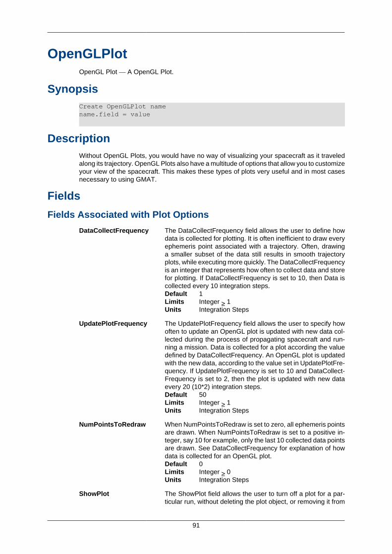
91
OpenGLPlotOpenGL Plot — A OpenGL Plot.
SynopsisCreate OpenGLPlot namename.field = value
DescriptionWithout OpenGL Plots, you would have no way of visualizing your spacecraft as it traveledalong its trajectory. OpenGL Plots also have a multitude of options that allow you to customizeyour view of the spacecraft. This makes these types of plots very useful and in most casesnecessary to using GMAT.
Fields
Fields Associated with Plot Options
DataCollectFrequency The DataCollectFrequency field allows the user to define howdata is collected for plotting. It is often inefficient to draw everyephemeris point associated with a trajectory. Often, drawinga smaller subset of the data still results in smooth trajectoryplots, while executing more quickly. The DataCollectFrequencyis an integer that represents how often to collect data and storefor plotting. If DataCollectFrequency is set to 10, then Data iscollected every 10 integration steps.Default 1Limits Integer ≥ 1Units Integration Steps
UpdatePlotFrequency The UpdatePlotFrequency field allows the user to specify howoften to update an OpenGL plot is updated with new data col-lected during the process of propagating spacecraft and run-ning a mission. Data is collected for a plot according the valuedefined by DataCollectFrequency. An OpenGL plot is updatedwith the new data, according to the value set in UpdatePlotFre-quency. If UpdatePlotFrequency is set to 10 and DataCollect-Frequency is set to 2, then the plot is updated with new dataevery 20 (10*2) integration steps.Default 50Limits Integer ≥ 1Units Integration Steps
NumPointsToRedraw When NumPointsToRedraw is set to zero, all ephemeris pointsare drawn. When NumPointsToRedraw is set to a positive in-teger, say 10 for example, only the last 10 collected data pointsare drawn. See DataCollectFrequency for explanation of howdata is collected for an OpenGL plot.Default 0Limits Integer ≥ 0Units Integration Steps
ShowPlot The ShowPlot field allows the user to turn off a plot for a par-ticular run, without deleting the plot object, or removing it from
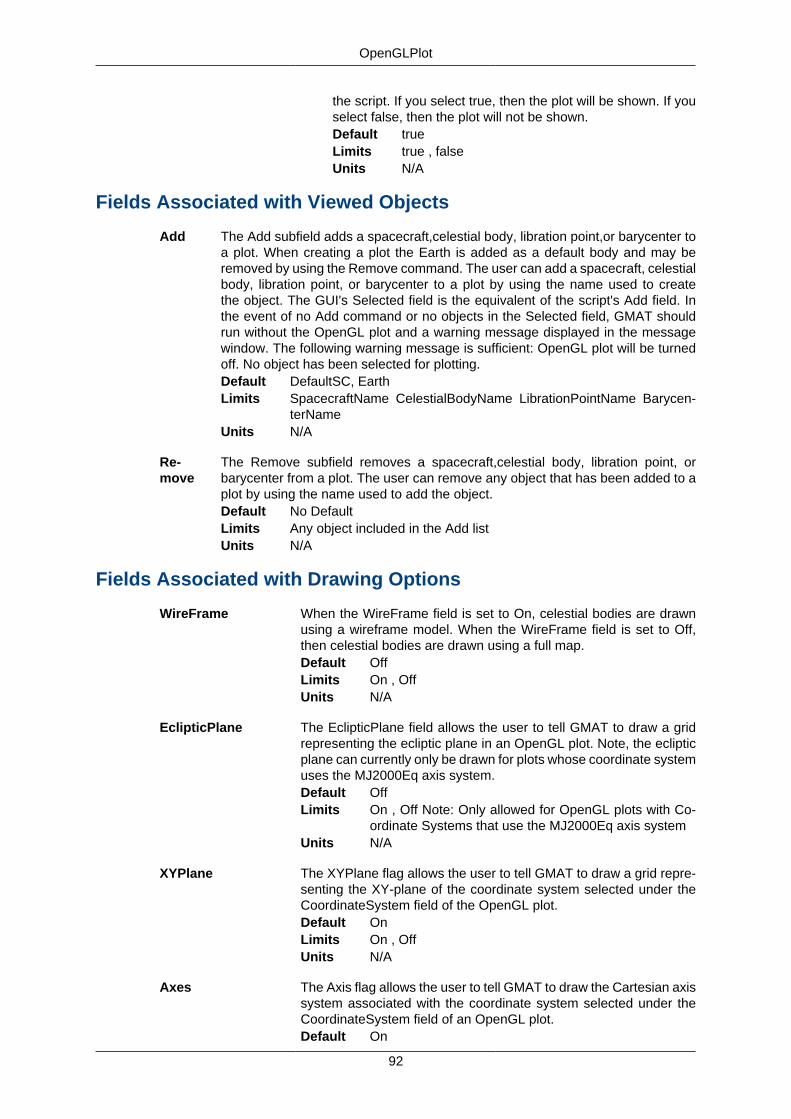
OpenGLPlot
92
the script. If you select true, then the plot will be shown. If youselect false, then the plot will not be shown.Default trueLimits true , falseUnits N/A
Fields Associated with Viewed Objects
Add The Add subfield adds a spacecraft,celestial body, libration point,or barycenter toa plot. When creating a plot the Earth is added as a default body and may beremoved by using the Remove command. The user can add a spacecraft, celestialbody, libration point, or barycenter to a plot by using the name used to createthe object. The GUI's Selected field is the equivalent of the script's Add field. Inthe event of no Add command or no objects in the Selected field, GMAT shouldrun without the OpenGL plot and a warning message displayed in the messagewindow. The following warning message is sufficient: OpenGL plot will be turnedoff. No object has been selected for plotting.Default DefaultSC, EarthLimits SpacecraftName CelestialBodyName LibrationPointName Barycen-
terNameUnits N/A
Re-move
The Remove subfield removes a spacecraft,celestial body, libration point, orbarycenter from a plot. The user can remove any object that has been added to aplot by using the name used to add the object.Default No DefaultLimits Any object included in the Add listUnits N/A
Fields Associated with Drawing Options
WireFrame When the WireFrame field is set to On, celestial bodies are drawnusing a wireframe model. When the WireFrame field is set to Off,then celestial bodies are drawn using a full map.Default OffLimits On , OffUnits N/A
EclipticPlane The EclipticPlane field allows the user to tell GMAT to draw a gridrepresenting the ecliptic plane in an OpenGL plot. Note, the eclipticplane can currently only be drawn for plots whose coordinate systemuses the MJ2000Eq axis system.Default OffLimits On , Off Note: Only allowed for OpenGL plots with Co-
ordinate Systems that use the MJ2000Eq axis systemUnits N/A
XYPlane The XYPlane flag allows the user to tell GMAT to draw a grid repre-senting the XY-plane of the coordinate system selected under theCoordinateSystem field of the OpenGL plot.Default OnLimits On , OffUnits N/A
Axes The Axis flag allows the user to tell GMAT to draw the Cartesian axissystem associated with the coordinate system selected under theCoordinateSystem field of an OpenGL plot.Default On
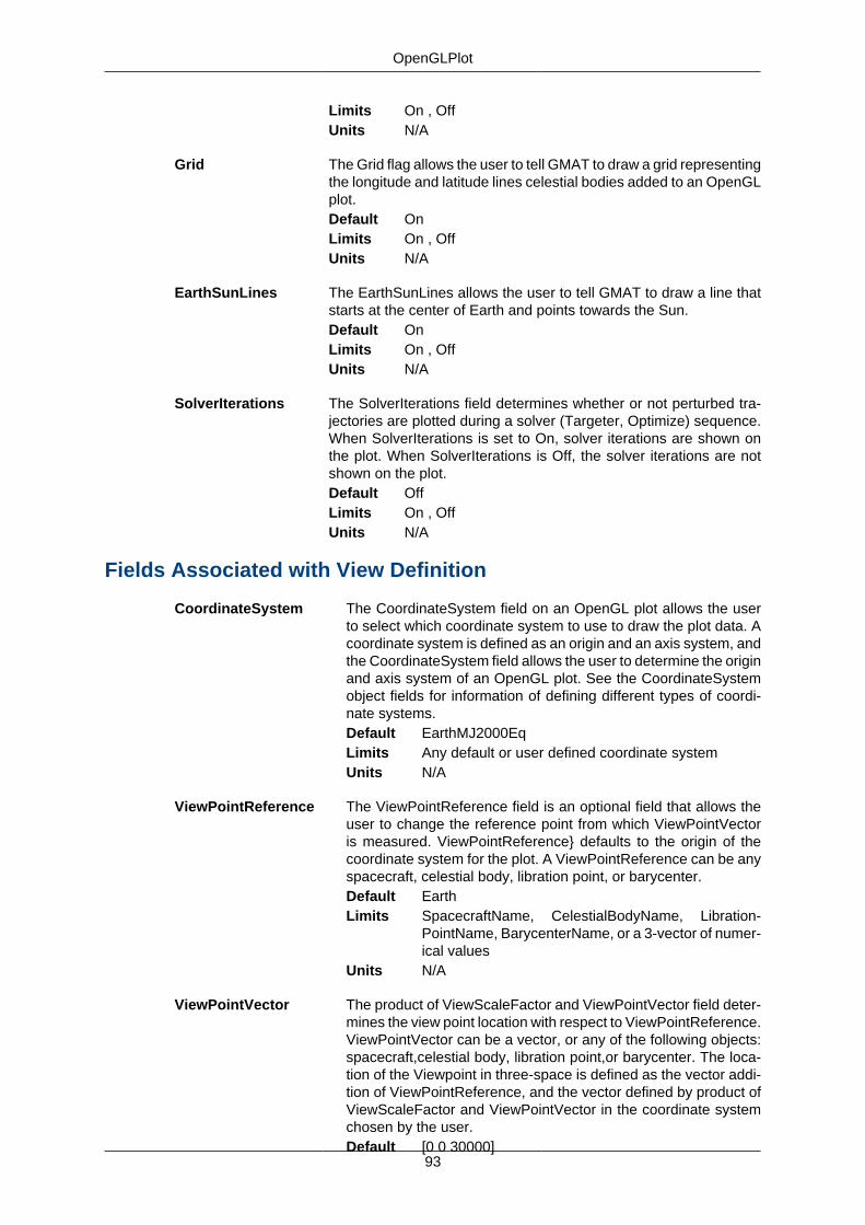
OpenGLPlot
93
Limits On , OffUnits N/A
Grid The Grid flag allows the user to tell GMAT to draw a grid representingthe longitude and latitude lines celestial bodies added to an OpenGLplot.Default OnLimits On , OffUnits N/A
EarthSunLines The EarthSunLines allows the user to tell GMAT to draw a line thatstarts at the center of Earth and points towards the Sun.Default OnLimits On , OffUnits N/A
SolverIterations The SolverIterations field determines whether or not perturbed tra-jectories are plotted during a solver (Targeter, Optimize) sequence.When SolverIterations is set to On, solver iterations are shown onthe plot. When SolverIterations is Off, the solver iterations are notshown on the plot.Default OffLimits On , OffUnits N/A
Fields Associated with View Definition
CoordinateSystem The CoordinateSystem field on an OpenGL plot allows the userto select which coordinate system to use to draw the plot data. Acoordinate system is defined as an origin and an axis system, andthe CoordinateSystem field allows the user to determine the originand axis system of an OpenGL plot. See the CoordinateSystemobject fields for information of defining different types of coordi-nate systems.Default EarthMJ2000EqLimits Any default or user defined coordinate systemUnits N/A
ViewPointReference The ViewPointReference field is an optional field that allows theuser to change the reference point from which ViewPointVectoris measured. ViewPointReference} defaults to the origin of thecoordinate system for the plot. A ViewPointReference can be anyspacecraft, celestial body, libration point, or barycenter.Default EarthLimits SpacecraftName, CelestialBodyName, Libration-
PointName, BarycenterName, or a 3-vector of numer-ical values
Units N/A
ViewPointVector The product of ViewScaleFactor and ViewPointVector field deter-mines the view point location with respect to ViewPointReference.ViewPointVector can be a vector, or any of the following objects:spacecraft,celestial body, libration point,or barycenter. The loca-tion of the Viewpoint in three-space is defined as the vector addi-tion of ViewPointReference, and the vector defined by product ofViewScaleFactor and ViewPointVector in the coordinate systemchosen by the user.Default [0 0 30000]
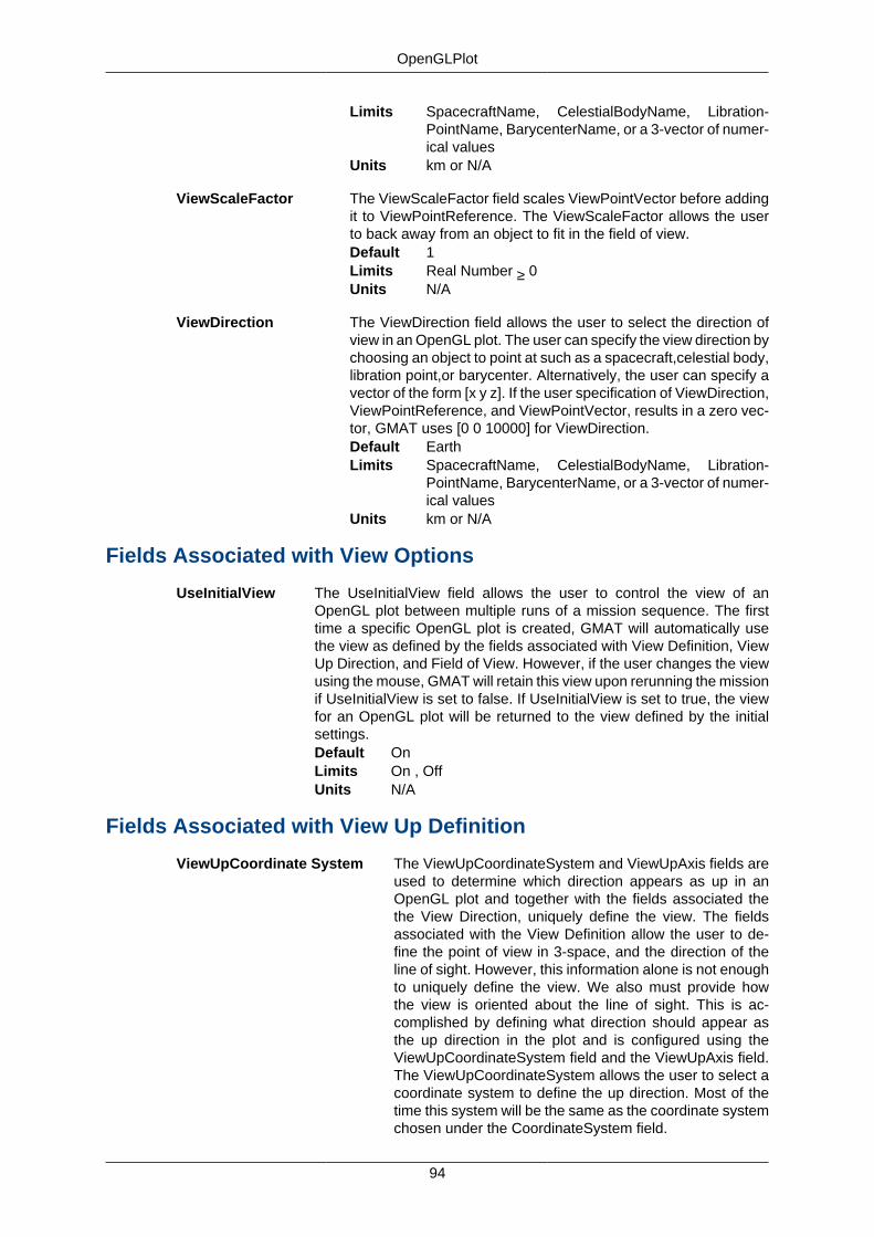
OpenGLPlot
94
Limits SpacecraftName, CelestialBodyName, Libration-PointName, BarycenterName, or a 3-vector of numer-ical values
Units km or N/A
ViewScaleFactor The ViewScaleFactor field scales ViewPointVector before addingit to ViewPointReference. The ViewScaleFactor allows the userto back away from an object to fit in the field of view.Default 1Limits Real Number ≥ 0Units N/A
ViewDirection The ViewDirection field allows the user to select the direction ofview in an OpenGL plot. The user can specify the view direction bychoosing an object to point at such as a spacecraft,celestial body,libration point,or barycenter. Alternatively, the user can specify avector of the form [x y z]. If the user specification of ViewDirection,ViewPointReference, and ViewPointVector, results in a zero vec-tor, GMAT uses [0 0 10000] for ViewDirection.Default EarthLimits SpacecraftName, CelestialBodyName, Libration-
PointName, BarycenterName, or a 3-vector of numer-ical values
Units km or N/A
Fields Associated with View Options
UseInitialView The UseInitialView field allows the user to control the view of anOpenGL plot between multiple runs of a mission sequence. The firsttime a specific OpenGL plot is created, GMAT will automatically usethe view as defined by the fields associated with View Definition, ViewUp Direction, and Field of View. However, if the user changes the viewusing the mouse, GMAT will retain this view upon rerunning the missionif UseInitialView is set to false. If UseInitialView is set to true, the viewfor an OpenGL plot will be returned to the view defined by the initialsettings.Default OnLimits On , OffUnits N/A
Fields Associated with View Up Definition
ViewUpCoordinate System The ViewUpCoordinateSystem and ViewUpAxis fields areused to determine which direction appears as up in anOpenGL plot and together with the fields associated thethe View Direction, uniquely define the view. The fieldsassociated with the View Definition allow the user to de-fine the point of view in 3-space, and the direction of theline of sight. However, this information alone is not enoughto uniquely define the view. We also must provide howthe view is oriented about the line of sight. This is ac-complished by defining what direction should appear asthe up direction in the plot and is configured using theViewUpCoordinateSystem field and the ViewUpAxis field.The ViewUpCoordinateSystem allows the user to select acoordinate system to define the up direction. Most of thetime this system will be the same as the coordinate systemchosen under the CoordinateSystem field.
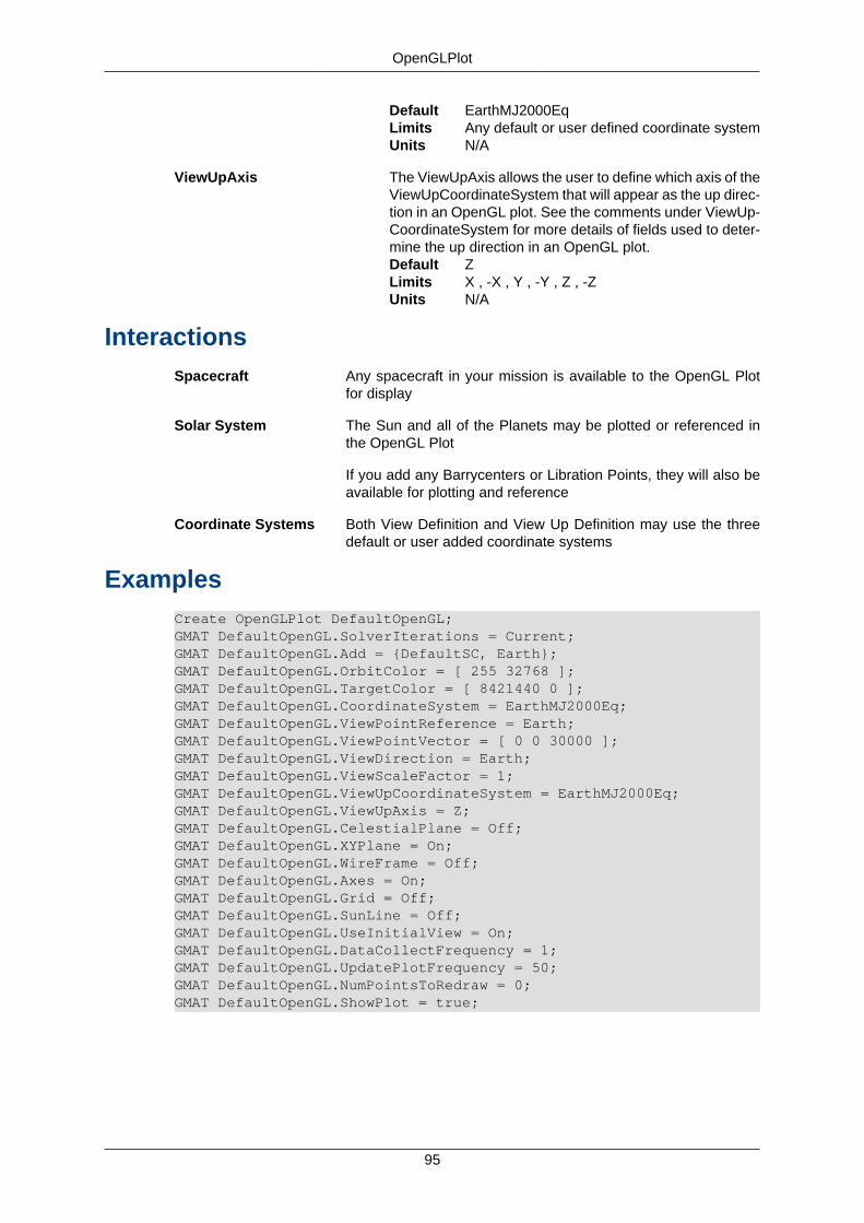
OpenGLPlot
95
Default EarthMJ2000EqLimits Any default or user defined coordinate systemUnits N/A
ViewUpAxis The ViewUpAxis allows the user to define which axis of theViewUpCoordinateSystem that will appear as the up direc-tion in an OpenGL plot. See the comments under ViewUp-CoordinateSystem for more details of fields used to deter-mine the up direction in an OpenGL plot.Default ZLimits X , -X , Y , -Y , Z , -ZUnits N/A
InteractionsSpacecraft Any spacecraft in your mission is available to the OpenGL Plot
for display
Solar System The Sun and all of the Planets may be plotted or referenced inthe OpenGL Plot
If you add any Barrycenters or Libration Points, they will also beavailable for plotting and reference
Coordinate Systems Both View Definition and View Up Definition may use the threedefault or user added coordinate systems
ExamplesCreate OpenGLPlot DefaultOpenGL;GMAT DefaultOpenGL.SolverIterations = Current;GMAT DefaultOpenGL.Add = {DefaultSC, Earth};GMAT DefaultOpenGL.OrbitColor = [ 255 32768 ];GMAT DefaultOpenGL.TargetColor = [ 8421440 0 ];GMAT DefaultOpenGL.CoordinateSystem = EarthMJ2000Eq;GMAT DefaultOpenGL.ViewPointReference = Earth;GMAT DefaultOpenGL.ViewPointVector = [ 0 0 30000 ];GMAT DefaultOpenGL.ViewDirection = Earth;GMAT DefaultOpenGL.ViewScaleFactor = 1;GMAT DefaultOpenGL.ViewUpCoordinateSystem = EarthMJ2000Eq;GMAT DefaultOpenGL.ViewUpAxis = Z;GMAT DefaultOpenGL.CelestialPlane = Off;GMAT DefaultOpenGL.XYPlane = On;GMAT DefaultOpenGL.WireFrame = Off;GMAT DefaultOpenGL.Axes = On;GMAT DefaultOpenGL.Grid = Off;GMAT DefaultOpenGL.SunLine = Off;GMAT DefaultOpenGL.UseInitialView = On;GMAT DefaultOpenGL.DataCollectFrequency = 1;GMAT DefaultOpenGL.UpdatePlotFrequency = 50;GMAT DefaultOpenGL.NumPointsToRedraw = 0;GMAT DefaultOpenGL.ShowPlot = true;
96
PropagatorPropagator — A propagator.
SynopsisCreate Propagator namename.field = value
DescriptionIn GMAT, a Propagator is a combination of an integrator and a force model. Hence, a Prop-agator contains a physical model of the space environment that is used to model the motionof a spacecraft as it moves forwards or backwards in time (VOP formulation is not current-ly supported). You configure a Propagator by selecting among different numerical integra-tors and environment models to create a Propagator appropriate to the flight regime of yourspacecraft during its mission. GMAT supports numerous numerical integrators as well asForce Models like point mass and non-spherical gravity, atmospheric drag (Earth), and solarradiation pressure.
To propagate spacecraft in GMAT, you first create and configure a Propagator object inthe script or in the Resource Tree. Then, in the mission sequence, you create a Propagatecommand, the topic of another section, and select among previously existing Propagatorsand Spacecraft. Hence, a Propagator is different from a Propagate command: A Propagatoris a resource and is found in the GUI under the resource tree, and a Propagate Event isconfigured under the Mission Tree and is how you instruct GMAT to propagate spacecraft.
InterfacesThe Propagator dialog box is illustrated below and contains two group boxes: the Integratorgroup and the Force Model group. This section discusses the items in each group on thePropagate Panel. It will present how to configure a propagator and discuss all possible usersettable fields in detail.
Integrator Group
The Integrator group allows you to select and configure a numerical integrator appropriateto your application. You select the type of numerical integrator in the -+Type+- pull-downmenu. After selecting the integrator type, the fields below the -+Type+- pull-down menu dy-namically configure to allow you to set relevant parameters for the selected integrator type.All integrators except for Adams-Bashforth-Moulton (ABM) are configured using the samefields. The ABM integrator has the following additional fields: -+MinIntegrationerror+- and -+NomIntegrationerror+-.
Force Model Group
The Force Model group allows you to configure a force model appropriate to the flight regimeof your application. The central body of propagation and error control method are also de-fined here. On a Propagator, GMAT classifies all celestial bodies into two mutually exclusivecategories: Primary Bodies, and Point Masses. Primary bodies can have a complex forcemodel that includes non-spherical gravity, drag, and magnetic field. Point mass bodies onlyhave a point-mass gravitational force.
You can add a Primary Body by clicking the Select button in the Primary Bodies group box.Once you have added a Primary Body (or mulitiple bodies in future versions), the pull downmenu allows you to configure the force model for each Primary Body. The text box, next to
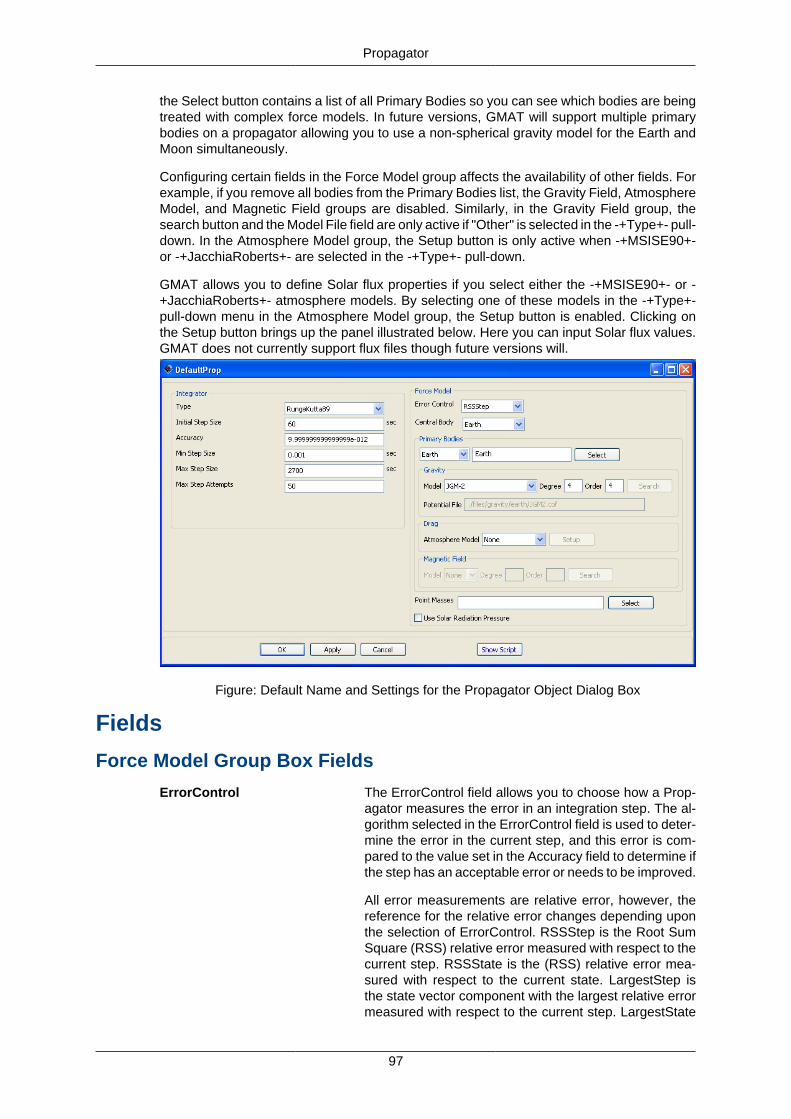
Propagator
97
the Select button contains a list of all Primary Bodies so you can see which bodies are beingtreated with complex force models. In future versions, GMAT will support multiple primarybodies on a propagator allowing you to use a non-spherical gravity model for the Earth andMoon simultaneously.
Configuring certain fields in the Force Model group affects the availability of other fields. Forexample, if you remove all bodies from the Primary Bodies list, the Gravity Field, AtmosphereModel, and Magnetic Field groups are disabled. Similarly, in the Gravity Field group, thesearch button and the Model File field are only active if "Other" is selected in the -+Type+- pull-down. In the Atmosphere Model group, the Setup button is only active when -+MSISE90+-or -+JacchiaRoberts+- are selected in the -+Type+- pull-down.
GMAT allows you to define Solar flux properties if you select either the -+MSISE90+- or -+JacchiaRoberts+- atmosphere models. By selecting one of these models in the -+Type+-pull-down menu in the Atmosphere Model group, the Setup button is enabled. Clicking onthe Setup button brings up the panel illustrated below. Here you can input Solar flux values.GMAT does not currently support flux files though future versions will.
Figure: Default Name and Settings for the Propagator Object Dialog Box
Fields
Force Model Group Box Fields
ErrorControl The ErrorControl field allows you to choose how a Prop-agator measures the error in an integration step. The al-gorithm selected in the ErrorControl field is used to deter-mine the error in the current step, and this error is com-pared to the value set in the Accuracy field to determine ifthe step has an acceptable error or needs to be improved.
All error measurements are relative error, however, thereference for the relative error changes depending uponthe selection of ErrorControl. RSSStep is the Root SumSquare (RSS) relative error measured with respect to thecurrent step. RSSState is the (RSS) relative error mea-sured with respect to the current state. LargestStep isthe state vector component with the largest relative errormeasured with respect to the current step. LargestState
Propagator
98
is the state vector component with the largest relative er-ror measured with respect to the current state. For a moredetailed discussion see the GMAT Mathematical Specifi-cation. Units: N/A.Default RSSStepLimits RSSStep, RSSState, LargestState,
LargestStep
CentralBody The CentralBody field allows the user to select the originfor the propagation. All propagation occurs in the FK5 ax-es system, about the CentralBody chosen by the user.The CentralBody must be a gravitational body and socannot be a LibrationPoint or other special point.Default EarthLimits Sun, Mercury, Venus, Earth, Luna, Mars,
Jupiter, Saturn, Uranus, Neptune, PlutoUnits N/A
PrimaryBodies The PrimaryBodies field is a list of all celestial bodiesthat are to be modelled with a force model more complexthan point mass gravity. Lists are surrounded by curlybraces. For each PrimaryBody, the user can choose adrag, magnetic field, and aspherical gravity model. Thereis a coupling between the PrimaryBodies filed and thePointMasses field. A primary body can be any planet ormoon not included in the PointMasses field.Default EarthLimits Sun, Mercury, Venus, Earth, Luna, Mars,
Jupiter, Saturn, Uranus, Neptune, PlutoUnits N/A
Gravity.PrimaryBody.PotentialFileThis field allows the user to define the source for the non-spherical gravity coefficients for a primary body. If a grav-ity file is located in the Primary Body's potential path asdefined in the startup file, you only need to specify themodel name and not the entire path. For example, if theJGM2 coefficients file is contained in the directory definedin the startup file by the line EARTH\_POT\_PATH, thenyou only need to specify the model name JGM2. If themodel is not contained in the body's potential path, youmust supply the entire path as well as the file name. IfGMAT does not successfully find the file requested, it us-es the default gravity model as defined in the startup file.From the GUI, only models for Earth appear if Earth is theactive primary body. This is to avoid allowing the user toselect a lunar potential model for the Earth. If the Otheroption is selected the user has the ability of selecting agravity model file on their local computer.Default JGM2Limits CentralBody-based models, Other. See
CommentsUnits N/A
Gravity.PrimaryBody.Degree This field allows the user to select the the degree, or num-ber of zonal terms, in the non-spherical gravity model. Ex.Gravity.Earth.Degree = 2 tells GMAT to use only the J2zonal term for the Earth. The value for Degree must beless than the maximum degree specified by the Model.Default 4
Propagator
99
Limits Integer >= 0 and < the maximum specified bythe model, Order <= Degree
Units N/A
Gravity.PrimaryBody.Order This field allows the user to select the the order, or num-ber of tesseral terms, in the non-spherical gravity model.Ex. Gravity.Earth.Order = 2 tells GMAT to use 2 tesseralterms. Note: Order must be greater than or equal to De-gree.Default 4Limits Integer >= 0 and < the maximum specified by
the model, Order <= DegreeUnits N/A
Drag The Drag field allows a user to specify a drag model. Cur-rently, only one drag model can be chosen for a particularpropagator and only Earth models are available.Default N/ALimits None, JacchiaRoberts, MSISE90, Exponen-
tialUnits N/A. Note: This field will be deprecated in fu-
ture versions of GMAT. Currently, the Dragfield and the Drag.AtmosphereModel fieldmust be set to the same value.
Drag.AtmosphereModel The Drag.AtmosphereModel field allows a user to speci-fy a drag model. Currently, only one drag model can bechosen for a particular propagator and only Earth modelsare available.Default NoneLimits None, JacchiaRoberts, MSISE90, Exponen-
tialUnits N/A
Drag.F107 The Drag.F107 field allows you to set the F10.7 solar fluxvalue used in computing atmospheric density. F10.7 is thesolar radiation at a wavelength of 10.7 cm.Default 150Limits Real Number >= 0Units W/m2/Hz
Drag.F107A The Drag.F107A field allows you to set the average F10.7value. F10.7 is the average of F10.7 over one month.Default 150Limits Real Number >= 0Units W/m2/Hz
Drag.MagneticIndex The Drag.MagneticIndex index field allows you to set thekp value for use in atmospheric density calculations. kpis a planetary 3-hour-average, geomagnetic index thatmeasures magnetic effects of solar radiation.Default 3Limits 0 <= Real Number <= 9Units N/A
PointMasses A PointMass is a planet or moon that is modelled by apoint source located at its center of gravity. A PointMassbody can be any planet or moon not included in the Pri-maryBodies field.Default None
Propagator
100
Limits Sun, Mercury, Venus, Earth, Luna, Mars,Jupiter, Saturn, Uranus, Neptune, Pluto
Units N/A
SRP The SRP field allows the user to include the force due tosolar radiation pressure in the total sum of forces.Default OffLimits On, OffUnits N/A
Integrator Group Box Fields
Type The Type field is used to set the type of numerical integrator.Default RungeKutta89Limits RungeKutta89, RungeKutta68, RungeKutta56, Prince-
Dormand45, PrinceDormand78, BulirschStoer, Adams-BashforthMoulton
InitialStepSize The InitialStepSize is the size of the first attempted step by the inte-grator. If the step defined by InitialStepSize does not satisfy Accuracy,the integrator adapts the step according an algorithm defined in themathematical specifications document to find an acceptable first stepthat meets the user's requested.Default 60 (sec)Limits Real NumberUnits seconds
Accuracy The Accuracy field is used to set the desired accuracy for an integra-tion step. When you set a value for Accuracy, GMAT uses the methodselected in ErrorControl field on the Force Model, to determine a met-ric of the accuracy. For each step, the integrator ensures that theaccuracy, as calculated using the method defined by ErrorControl,is less than the limit defined by Accuracy. If an integrator exceedsMaxStepAttempts trying to meet the requested accuracy, and errormessage is thrown and propagation stops.Default 1e-11Limits Real Number >= 0Units N/A
MinStep The MinStep field is used to set the minimum allowable step size.Default .001 (sec)Limits Real Number > 0, MinStep <= MaxStepUnits seconds
MaxStep The MaxStep field is used to set the maximum allowable step size.Default 2700.0 (sec)Limits Real Number > 0, MinStep <= MaxStepUnits seconds
MaxStepAttempts The MaxStepAttempts field allows the user to set the number of at-tempts the integrator takes to meet the tolerance defined by Accuracy.Default 50Limits Integer > 0Units None
Fields Associated Only with Adams-Bashforth-Moulton Integrator
MinIntegrationerror The MinIntegrationerror field is used by the ABM integrator (andother predictor-corrector integrators when implemented) as the
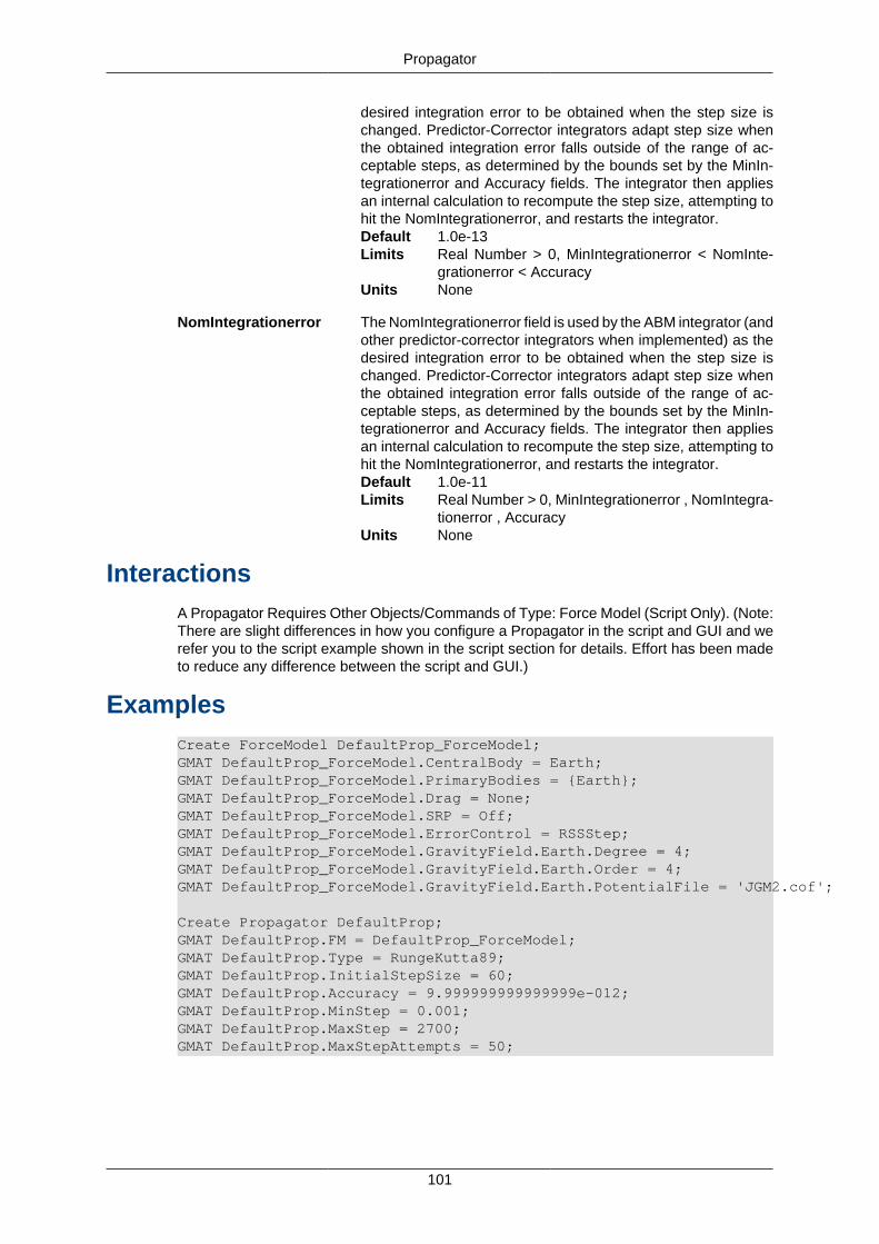
Propagator
101
desired integration error to be obtained when the step size ischanged. Predictor-Corrector integrators adapt step size whenthe obtained integration error falls outside of the range of ac-ceptable steps, as determined by the bounds set by the MinIn-tegrationerror and Accuracy fields. The integrator then appliesan internal calculation to recompute the step size, attempting tohit the NomIntegrationerror, and restarts the integrator.Default 1.0e-13Limits Real Number > 0, MinIntegrationerror < NomInte-
grationerror < AccuracyUnits None
NomIntegrationerror The NomIntegrationerror field is used by the ABM integrator (andother predictor-corrector integrators when implemented) as thedesired integration error to be obtained when the step size ischanged. Predictor-Corrector integrators adapt step size whenthe obtained integration error falls outside of the range of ac-ceptable steps, as determined by the bounds set by the MinIn-tegrationerror and Accuracy fields. The integrator then appliesan internal calculation to recompute the step size, attempting tohit the NomIntegrationerror, and restarts the integrator.Default 1.0e-11Limits Real Number > 0, MinIntegrationerror , NomIntegra-
tionerror , AccuracyUnits None
InteractionsA Propagator Requires Other Objects/Commands of Type: Force Model (Script Only). (Note:There are slight differences in how you configure a Propagator in the script and GUI and werefer you to the script example shown in the script section for details. Effort has been madeto reduce any difference between the script and GUI.)
ExamplesCreate ForceModel DefaultProp_ForceModel;GMAT DefaultProp_ForceModel.CentralBody = Earth;GMAT DefaultProp_ForceModel.PrimaryBodies = {Earth};GMAT DefaultProp_ForceModel.Drag = None;GMAT DefaultProp_ForceModel.SRP = Off;GMAT DefaultProp_ForceModel.ErrorControl = RSSStep;GMAT DefaultProp_ForceModel.GravityField.Earth.Degree = 4;GMAT DefaultProp_ForceModel.GravityField.Earth.Order = 4;GMAT DefaultProp_ForceModel.GravityField.Earth.PotentialFile = 'JGM2.cof';
Create Propagator DefaultProp;GMAT DefaultProp.FM = DefaultProp_ForceModel;GMAT DefaultProp.Type = RungeKutta89;GMAT DefaultProp.InitialStepSize = 60;GMAT DefaultProp.Accuracy = 9.999999999999999e-012;GMAT DefaultProp.MinStep = 0.001;GMAT DefaultProp.MaxStep = 2700;GMAT DefaultProp.MaxStepAttempts = 50;
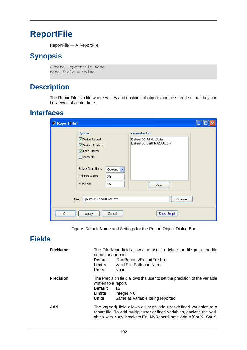
102
ReportFileReportFile — A ReportFile.
SynopsisCreate ReportFile namename.field = value
DescriptionThe ReportFile is a file where values and qualities of objects can be stored so that they canbe viewed at a later time.
Interfaces
Figure: Default Name and Settings for the Report Object Dialog Box
FieldsFileName The FileName field allows the user to define the file path and file
name for a report.Default /RunReports/ReportFile1.txtLimits Valid File Path and NameUnits None
Precision The Precision field allows the user to set the precision of the variablewritten to a report.Default 16Limits Integer > 0Units Same as variable being reported.
Add The \st{Add} field allows a userto add user-defined variables to areport file. To add multipleuser-defined variables, enclose the vari-ables with curly brackets.Ex. MyReportName.Add ={Sat.X, Sat.Y,
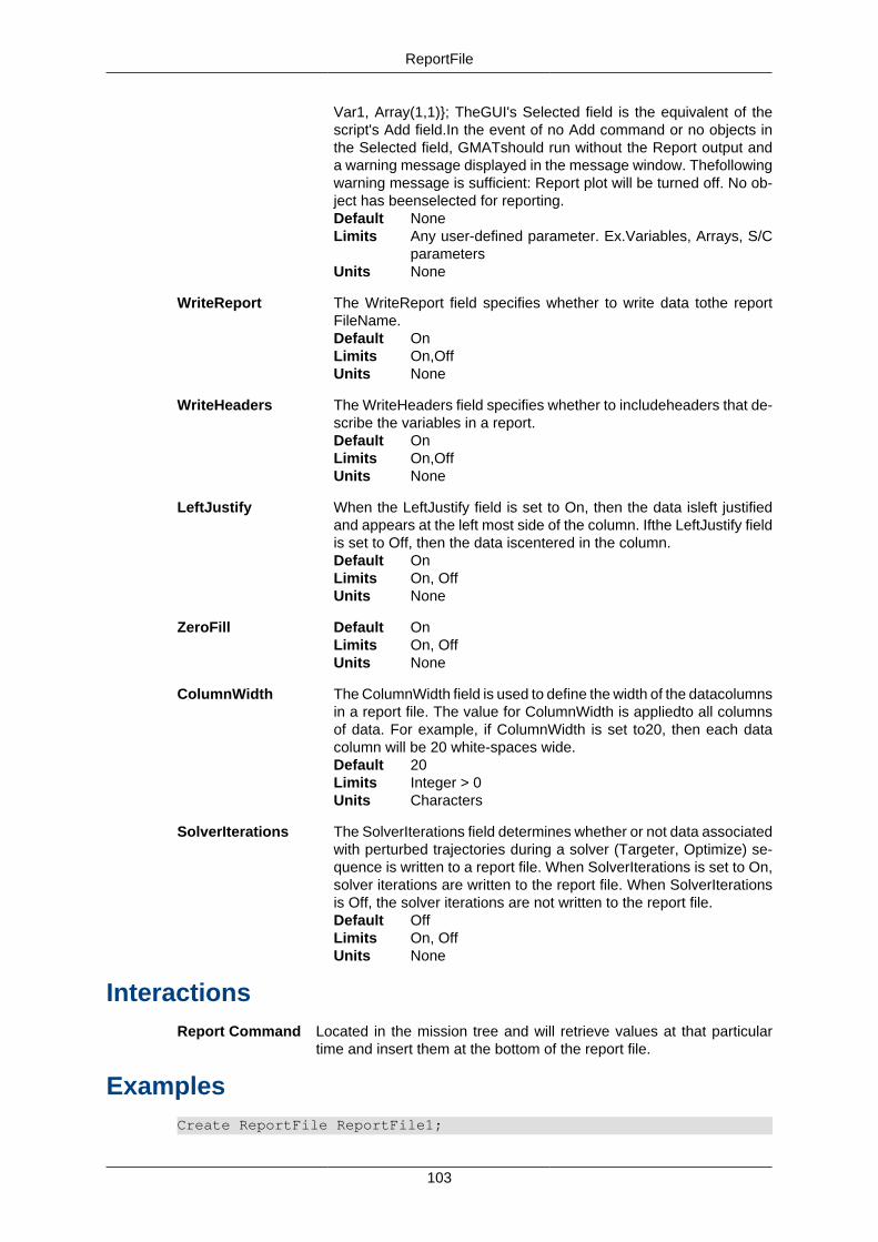
ReportFile
103
Var1, Array(1,1)}; TheGUI's Selected field is the equivalent of thescript's Add field.In the event of no Add command or no objects inthe Selected field, GMATshould run without the Report output anda warning message displayed in the message window. Thefollowingwarning message is sufficient: Report plot will be turned off. No ob-ject has beenselected for reporting.Default NoneLimits Any user-defined parameter. Ex.Variables, Arrays, S/C
parametersUnits None
WriteReport The WriteReport field specifies whether to write data tothe reportFileName.Default OnLimits On,OffUnits None
WriteHeaders The WriteHeaders field specifies whether to includeheaders that de-scribe the variables in a report.Default OnLimits On,OffUnits None
LeftJustify When the LeftJustify field is set to On, then the data isleft justifiedand appears at the left most side of the column. Ifthe LeftJustify fieldis set to Off, then the data iscentered in the column.Default OnLimits On, OffUnits None
ZeroFill Default OnLimits On, OffUnits None
ColumnWidth The ColumnWidth field is used to define the width of the datacolumnsin a report file. The value for ColumnWidth is appliedto all columnsof data. For example, if ColumnWidth is set to20, then each datacolumn will be 20 white-spaces wide.Default 20Limits Integer > 0Units Characters
SolverIterations The SolverIterations field determines whether or not data associatedwith perturbed trajectories during a solver (Targeter, Optimize) se-quence is written to a report file. When SolverIterations is set to On,solver iterations are written to the report file. When SolverIterationsis Off, the solver iterations are not written to the report file.Default OffLimits On, OffUnits None
InteractionsReport Command Located in the mission tree and will retrieve values at that particular
time and insert them at the bottom of the report file.
ExamplesCreate ReportFile ReportFile1;
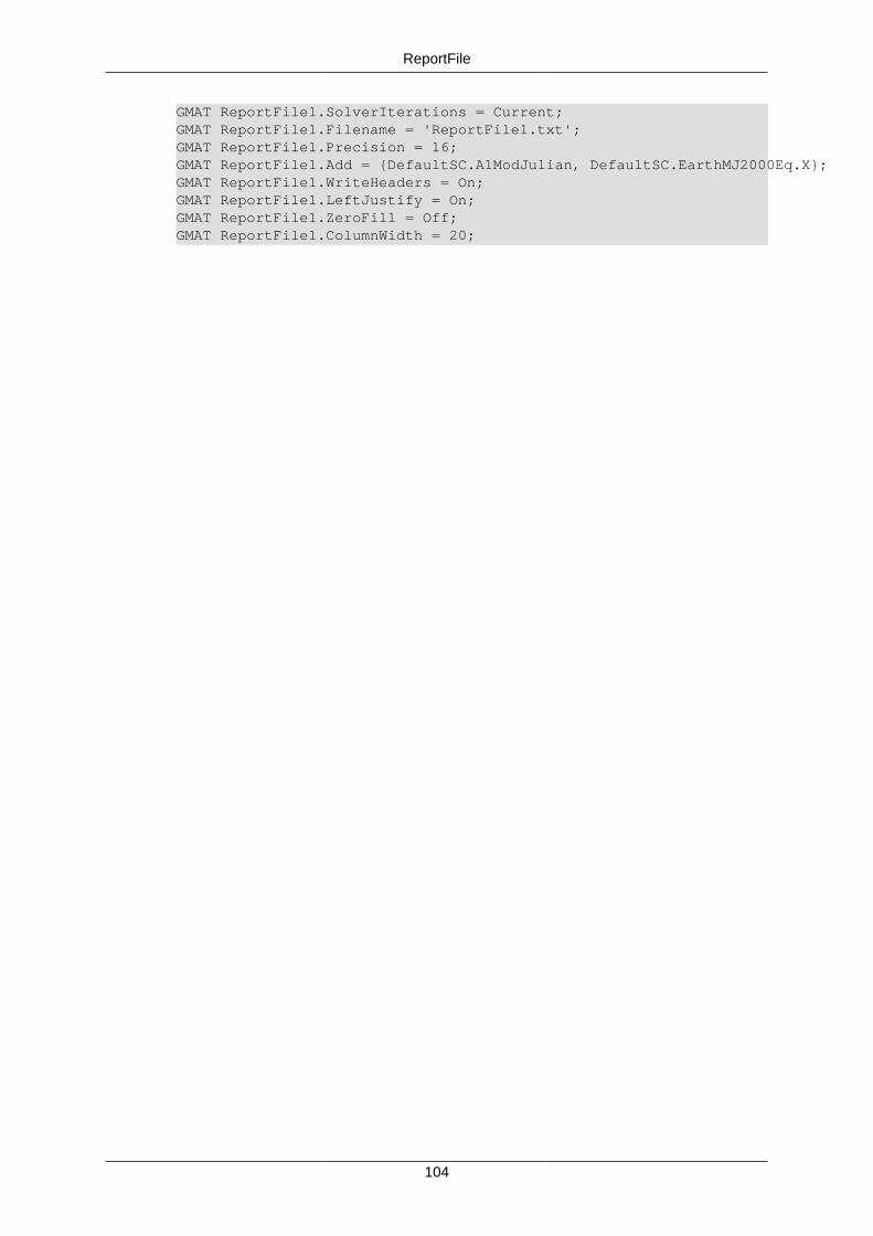
ReportFile
104
GMAT ReportFile1.SolverIterations = Current;GMAT ReportFile1.Filename = 'ReportFile1.txt';GMAT ReportFile1.Precision = 16;GMAT ReportFile1.Add = {DefaultSC.A1ModJulian, DefaultSC.EarthMJ2000Eq.X};GMAT ReportFile1.WriteHeaders = On;GMAT ReportFile1.LeftJustify = On;GMAT ReportFile1.ZeroFill = Off;GMAT ReportFile1.ColumnWidth = 20;
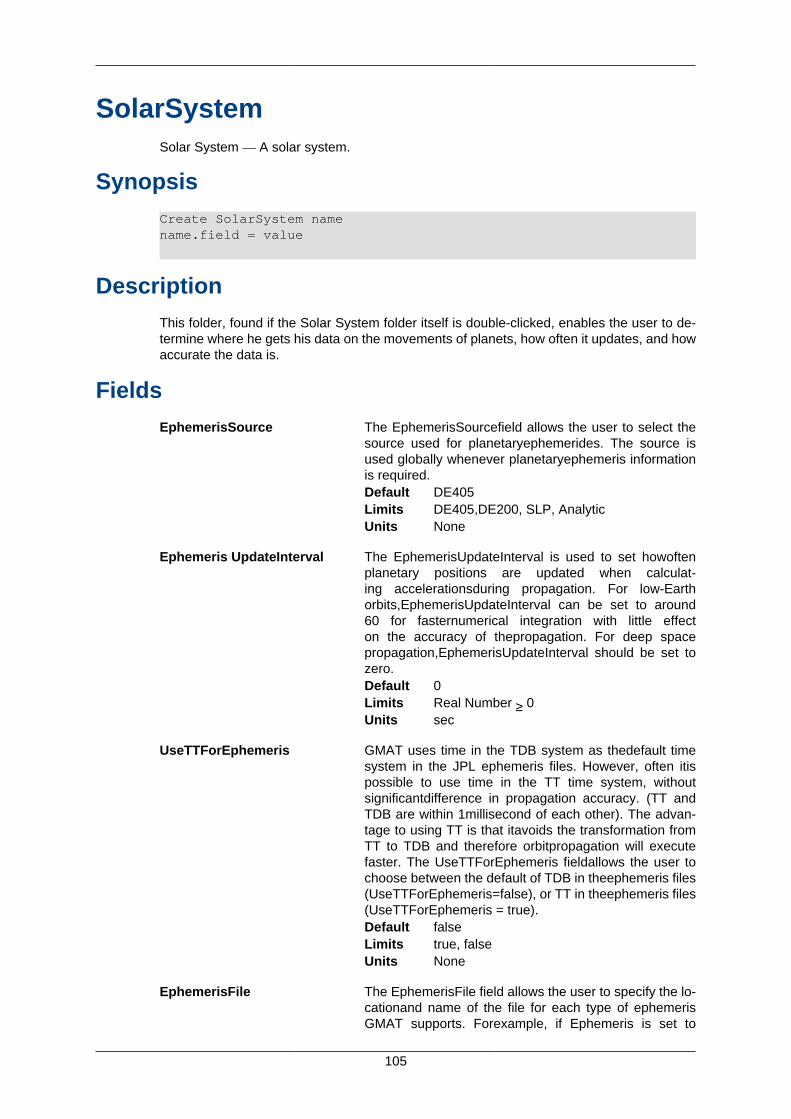
105
SolarSystemSolar System — A solar system.
SynopsisCreate SolarSystem namename.field = value
DescriptionThis folder, found if the Solar System folder itself is double-clicked, enables the user to de-termine where he gets his data on the movements of planets, how often it updates, and howaccurate the data is.
FieldsEphemerisSource The EphemerisSourcefield allows the user to select the
source used for planetaryephemerides. The source isused globally whenever planetaryephemeris informationis required.Default DE405Limits DE405,DE200, SLP, AnalyticUnits None
Ephemeris UpdateInterval The EphemerisUpdateInterval is used to set howoftenplanetary positions are updated when calculat-ing accelerationsduring propagation. For low-Earthorbits,EphemerisUpdateInterval can be set to around60 for fasternumerical integration with little effecton the accuracy of thepropagation. For deep spacepropagation,EphemerisUpdateInterval should be set tozero.Default 0Limits Real Number ≥ 0Units sec
UseTTForEphemeris GMAT uses time in the TDB system as thedefault timesystem in the JPL ephemeris files. However, often itispossible to use time in the TT time system, withoutsignificantdifference in propagation accuracy. (TT andTDB are within 1millisecond of each other). The advan-tage to using TT is that itavoids the transformation fromTT to TDB and therefore orbitpropagation will executefaster. The UseTTForEphemeris fieldallows the user tochoose between the default of TDB in theephemeris files(UseTTForEphemeris=false), or TT in theephemeris files(UseTTForEphemeris = true).Default falseLimits true, falseUnits None
EphemerisFile The EphemerisFile field allows the user to specify the lo-cationand name of the file for each type of ephemerisGMAT supports. Forexample, if Ephemeris is set to

SolarSystem
106
DE405, you can set thepath for a DE405 file usingSolarSystem.EphemerisFile =c:/MyPath/MyDE405.file.Default Same as startup file.Limits Filepath and file name consistent with oper-
ating systemUnits None
AnalyticModel Default LowFidelityLimits LowFidelityUnits None
InteractionsCelestialBodies, BaryCenter,and Libration Point
The position and data on all these depend on the sourceof the Solar System data and how often it is updated.
Propagator How often the position of the planetary bodies are updat-ed will have an impact on how a spacecraft will propagate.
Spacecraft A number of parameters of a spacecraft are based off theposition of the planets
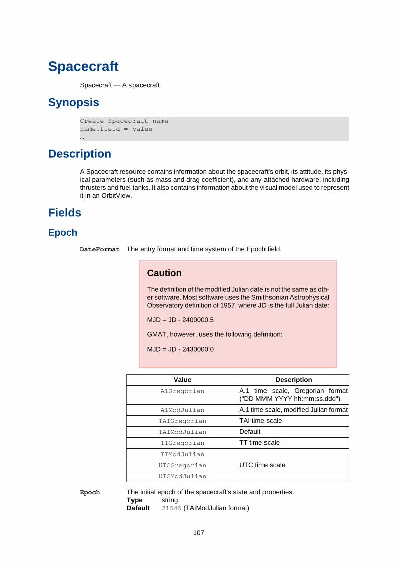
107
SpacecraftSpacecraft — A spacecraft
SynopsisCreate Spacecraft namename.field = value…
DescriptionA Spacecraft resource contains information about the spacecraft's orbit, its attitude, its phys-ical parameters (such as mass and drag coefficient), and any attached hardware, includingthrusters and fuel tanks. It also contains information about the visual model used to representit in an OrbitView.
Fields
Epoch
DateFormat The entry format and time system of the Epoch field.
Caution
The definition of the modified Julian date is not the same as oth-er software. Most software uses the Smithsonian AstrophysicalObservatory definition of 1957, where JD is the full Julian date:
MJD = JD - 2400000.5
GMAT, however, uses the following definition:
MJD = JD - 2430000.0
Value Description
A1Gregorian A.1 time scale, Gregorian format("DD MMM YYYY hh:mm:ss.ddd")
A1ModJulian A.1 time scale, modified Julian format
TAIGregorian TAI time scale
TAIModJulian Default
TTGregorian TT time scale
TTModJulian
UTCGregorian UTC time scale
UTCModJulian
Epoch The initial epoch of the spacecraft's state and properties.Type stringDefault 21545 (TAIModJulian format)
Spacecraft
108
Limits 04 Oct 1957 12:00:00.000 or later in all time systems(6116.0 modified Julian)
Units days (modified Julian format only)
Orbit
CoordinateSystem The Coordinate System field allows the user to choose which coor-dinate system with which to define the orbit state vector. The Coordi-nate System field has a dependency upon the State Type field. If thecoordinate system chosen by the user does not have a gravitationalbody at the origin, then the state types Keplerian, ModifiedKeplerian,and Equinoctial are not permitted. This is because these state typesrequire a µ value.Type enumerationValues • EarthMJ2000Eq (default)
• EarthMJ2000Ec• EarthFixed• any user-defined coordinate system
DisplayStateType The State Type field allows the user to configure the type of statevector that they wish to use. The State Type field has a dependencyupon the Coordinate System field. If the coordinate system chosenby the user does not have a gravitational body at the origin, thenthe state types Keplerian, ModifiedKeplerian, and Equinoctial are notpermitted. This is because these state types require a µ value.Type enumerationValues • Cartesian (default)
• Keplerian• ModifiedKeplerian• SphericalAZFPA• SphericalRADEC• Equinoctial
Cartesian State
X X is the x-component of the Spacecraft state in the coordinate system chosen in theSpacecraft Coordinate System field.Type real numberDefault 7100LimitsUnits km
Y Y is the y-component of the Spacecraft state in the coordinate system chosen in theSpacecraft Coordinate System field.Type real numberDefault 0LimitsUnits km
Z Z is the z-component of the Spacecraft state in the coordinate system chosen in theSpacecraft Coordinate System field.Type real numberDefault 1300LimitsUnits km
VX VX is the x-component of the Spacecraft velocity in the coordinate system chosen inthe Spacecraft Coordinate System field.Type real number
Spacecraft
109
Default 0LimitsUnits km
VY VY is the y-component of the Spacecraft velocity in the coordinate system chosen inthe Spacecraft Coordinate System field.Type real numberDefault 7.35LimitsUnits km
VZ VZ is the z-component of the Spacecraft velocity in the coordinate system chosen inthe Spacecraft Coordinate System field.Type real numberDefault 1LimitsUnits km
Keplerian State
SMA The SMA field is the spacecraft orbit's osculating Keplerian semimajor axis in thecoordinate system chosen in the Spacecraft Coordinate System field. SMA must bestrictly greater than 1 m or less than -1 m to avoid numerical issues in the conversionsto other state types. For circular and elliptical orbits ( 0 <= ECC < 0.9999999 ) SMAshould only be greater than 1 m and for hyperbolic orbits (ECC > 1.0000001) SMAshould be less than -1 m. GMAT does not support the creation of parabolic orbits.Type real numberDefaultLimits |SMA| > 1e-3 kmUnits km
ECC The ECC field is the spacecraft orbit's osculating eccentricity. For circular or ellipticorbits, ECC must be greater than or equal to 0.0, and less than or equal to 0.9999999to avoid numerical issues in the conversion to other state types as the Keplerian el-ements are undefined for parabolic orbits. For hyperbolic orbits ECC must be greaterthan or equal to 1.0000001. See also the SMA description.Type real numberDefaultLimits 0.0 <= ECC <= 0.9999999 or ECC >= 1.0000001Units none
INC The INC field is the spacecraft orbit's osculating inclination, in degrees, with respectto the selected coordinate system.Type real numberDefaultLimitsUnits degrees
RAAN The RAAN field is the spacecraft orbit's osculating right ascension of the ascendingnode, in degrees, with respect to the selected coordinate system.Type real numberDefaultLimitsUnits degrees
AOP The AOP field is the spacecraft orbit's osculating argument of periapsis, in degrees,with respect to the selected coordinate system.Type real numberDefault
Spacecraft
110
LimitsUnits degrees
TA The TA field is the spacecraft orbit's osculating true anomaly.Type real numberDefaultLimitsUnits degrees
ModifiedKeplerian State
RadPer The RadPer field is the spacecraft orbit's osculating radius of periapsis. RadPermust be greater than zero.
Type real number
Default
Limits RadPer > 0
Units km
RadApo The RadApo field is the spacecraft orbit's osculating radius of apoapsis. RadApomust be strictly greater than or less than zero. When RadApo is negative, the orbitis hyperbolic.
Type real number
Default
Limits
Units km
INC See the the section called “Keplerian State” section for a description of this field.
RAAN See the the section called “Keplerian State” section for a description of this field.
AOP See the the section called “Keplerian State” section for a description of this field.
TA See the the section called “Keplerian State” section for a description of this field.
SphericalAZFPA State
RMAG The RMAG field allows the user to set the magnitude of the spacecraft's positionvector.
Type real number
Default
Limits
Units km
RA The RA field allows the user to set the spacecraft's right ascension.
Type real number
Default
Limits
Spacecraft
111
Units degrees
DEC The DEC field allows the user to set the spacecraft's declination.
Type real number
Default
Limits
Units degrees
VMAG The VMAG field allows the user to set the magnitude of the spacecraft's velocity.
Type real number
Default
Limits VMAG >= 0
Units
AZI The AZI field allows the user to set the spacecraft's azimuth angle.
Type real number
Default
Limits
Units degrees
FPA The FPA allows the user to set a spacecraft's flight path angle.
Type real number
Default
Limits
Units degrees
Examples
Example 9. Creating a default Spacecraft
Create Spacecraft sc;
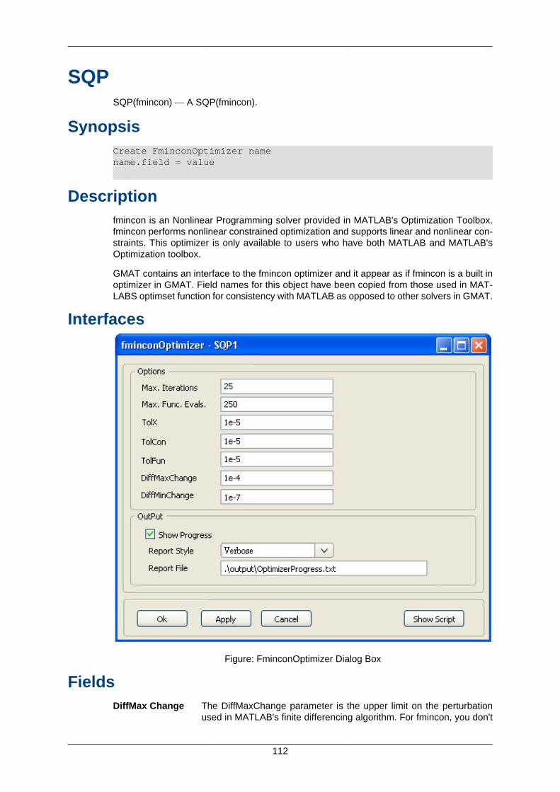
112
SQPSQP(fmincon) — A SQP(fmincon).
SynopsisCreate FminconOptimizer namename.field = value
Descriptionfmincon is an Nonlinear Programming solver provided in MATLAB's Optimization Toolbox.fmincon performs nonlinear constrained optimization and supports linear and nonlinear con-straints. This optimizer is only available to users who have both MATLAB and MATLAB'sOptimization toolbox.
GMAT contains an interface to the fmincon optimizer and it appear as if fmincon is a built inoptimizer in GMAT. Field names for this object have been copied from those used in MAT-LABS optimset function for consistency with MATLAB as opposed to other solvers in GMAT.
Interfaces
Figure: FminconOptimizer Dialog Box
FieldsDiffMax Change The DiffMaxChange parameter is the upper limit on the perturbation
used in MATLAB's finite differencing algorithm. For fmincon, you don't
SQP
113
specify a single perturbation value, but rather give MATLAB a range,and it uses an adaptive algorithm that attempts to find the optimal per-turbation.Default 0.1Limits Real Number > 0Units None
DiffMin Change The DiffMinChange parameter is the lower limit on the perturbationused in MATLAB's finite differencing algorithm. For fmincon, you don'tspecify a single perturbation value, but rather give MATLAB a range,and it uses an adaptive algorithm that attempts to find the optimal per-turbatin.Default 1e-8Limits Real Number > 0Units None
MaxFunEvals The MaxFunEvals parameter allows the user to set the maximum num-ber of cost function evaluations in an attempt to find an optimal solution.This is equivalent to setting the maximum number of passes throughan optimization loop in a GMAT script. If a solution is not found beforethe maximum function evaluations, fmincon outputs an ExitFlag of ze-ro, and GMAT continues.Default 1000Limits Integer > 0Units None
MaxIter The MaxIter parameter allows the user to set the maximum allowablenumber of optimizer iterations. Depending upon the nature of the prob-lem, and whether gradients are provided, it may take many functionevaluations for each optimizer iteration. The MaxIter parameter allowsthe user to control the maximum function evaluations, and maximumiterations independently.Default 400Limits Integer > 0Units None
TolX The TolX parameter is the termination toler-ance on the vector of inde-pendent variables, and is used only if the user sets a value.Default 1e-4Limits Real Number > 0Units None
TolFun The TolFun parameter is the convergence tolerance on the cost func-tion value.Default 1e-4Limits Real Number > 0Units None
TolCon The TolCon parameter is the convergence tolerance on the constraintfunctions.Default 1e-4Limits Real Number > 0Units None
ShowProgress The ShowProgress field determines whether data pertaining to itera-tions of the solver is displayed in the message window. When Show-Progress is true, the amount of information contained in the messagewindow is controlled by the ReportSytle field.Default true
SQP
114
Limits true, falseUnits None
ReportStyle The ReportStyel field determines the amount and type of data writtento the message window for each iteration of the solver (When Show-Progress is true). ADD DESCRIPTIONS OF CONCISE,VERBOSE,ADN NORMAL. I CAN'T RUN THE OPTIMIZER RIGHT NOW SO ICAN'T TELL WHAT EACH SETTING DOES.Default NormalLimits Normal, Concise, Verbose, DebugUnits None
ReportFile The ReportFile field contains the path and file name of the report file.Default NormalLimits .\output\OptimizerData.txtUnits None
Using an fminconOptimizer• Optimize Command
• Minimize
• Nonlinear Constraint
ExamplesCreate FminconOptimizer SQP1;GMAT SQP1.MaxIter = 25;GMAT SQP1.MaxFunEvals = 250;GMAT SQP1.TolX = 1e-5;GMAT SQP1.TolFun = 1e-5;GMAT SQP1.TolCon = 1e-5;GMAT SQP1.DiffMaxChange = 1e-4;GMAT SQP1.DiffMinChange = 1e-7;GMAT SQP1.ShowProgress = true;GMAT SQP1.ReportStyle = 'Verbose';GMAT SQP1.ReportFile = '\output\OptimizerProgress.txt';
115
StringString — A string.
SynopsisCreate String namename.field = value
DescriptionThis page will show you how to create and use String objects. Stings are useful for storingcharacters as a set. One possible use of them is to report back a specific message at a setpoint in the mission sequence.
InteractionsReportFile You may add a string to the Parameter List in the Report Object dialog
box via the ParameterSelectDialog box.
Report Command Alternatively, you may add a string to the Parameter List in the ReportCommand dialog box
Using the Script
Script Syntax
GMAT String Name = String;
Script Examples
% The following is an example String declarationGMAT Example = hello world;
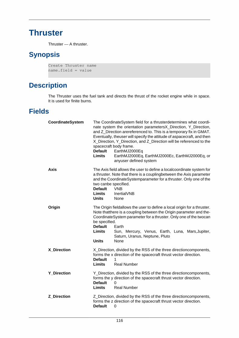
116
ThrusterThruster — A thruster.
SynopsisCreate Thruster namename.field = value
DescriptionThe Thruster uses the fuel tank and directs the thrust of the rocket engine while in space.It is used for finite burns.
FieldsCoordinateSystem The CoordinateSystem field for a thrusterdetermines what coordi-
nate system the orientation parametersX_Direction, Y_Direction,and Z_Direction arereferenced to. This is a temporary fix in GMAT.Eventually, theuser will specify the attitude of aspacecraft, and thenX_Direction, Y_Direction, and Z_Direction will be referenced to thespacecraft body frame.Default EarthMJ2000EqLimits EarthMJ2000Eq, EarthMJ2000Ec, EarthMJ2000Eq, or
anyuser defined system
Axis The Axis field allows the user to define a localcoordinate system fora thruster. Note that there is a couplingbetween the Axis parameterand the CoordinateSystemparameter for a thruster. Only one of thetwo canbe specified.Default VNBLimits InertialVNBUnits None
Origin The Origin fieldallows the user to define a local origin for a thruster.Note thatthere is a coupling between the Origin parameter and the-CoordinateSystem parameter for a thruster. Only one of the twocanbe specified.Default EarthLimits Sun, Mercury, Venus, Earth, Luna, Mars,Jupiter,
Saturn, Uranus, Neptune, PlutoUnits None
X_Direction X_Direction, divided by the RSS of the three directioncomponents,forms the x direction of the spacecraft thrust vector direction.Default 1Limits Real Number
Y_Direction Y_Direction, divided by the RSS of the three directioncomponents,forms the y direction of the spacecraft thrust vector direction.Default 0Limits Real Number
Z_Direction Z_Direction, divided by the RSS of the three directioncomponents,forms the z direction of the spacecraft thrust vector direction.Default 0
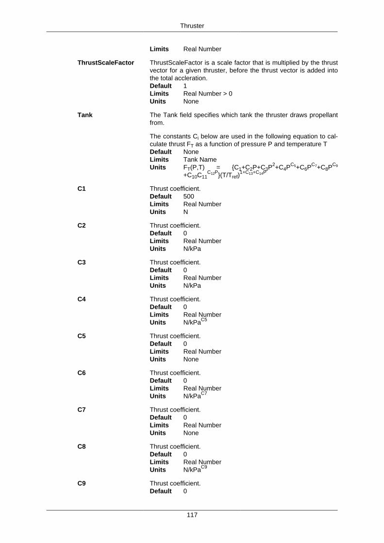
Thruster
117
Limits Real Number
ThrustScaleFactor ThrustScaleFactor is a scale factor that is multiplied by the thrustvector for a given thruster, before the thrust vector is added intothe total accleration.Default 1Limits Real Number > 0Units None
Tank The Tank field specifies which tank the thruster draws propellantfrom.
The constants Ci below are used in the following equation to cal-culate thrust FT as a function of pressure P and temperature TDefault NoneLimits Tank NameUnits FT(P,T) = {C1+C2P+C3P2+C4PC5+C6PC7+C8PC9
+C10C11C12P}(T/Tref)
1+C13+C14P
C1 Thrust coefficient.Default 500Limits Real NumberUnits N
C2 Thrust coefficient.Default 0Limits Real NumberUnits N/kPa
C3 Thrust coefficient.Default 0Limits Real NumberUnits N/kPa
C4 Thrust coefficient.Default 0Limits Real NumberUnits N/kPaC5
C5 Thrust coefficient.Default 0Limits Real NumberUnits None
C6 Thrust coefficient.Default 0Limits Real NumberUnits N/kPaC7
C7 Thrust coefficient.Default 0Limits Real NumberUnits None
C8 Thrust coefficient.Default 0Limits Real NumberUnits N/kPaC9
C9 Thrust coefficient.Default 0
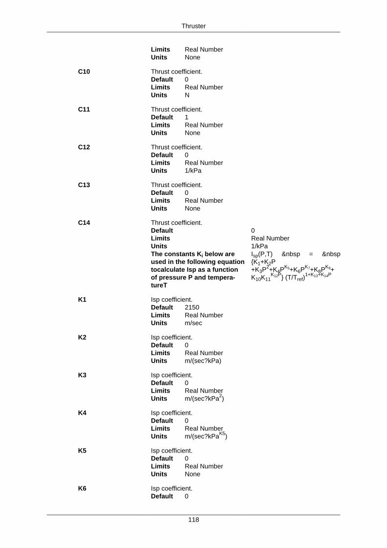
Thruster
118
Limits Real NumberUnits None
C10 Thrust coefficient.Default 0Limits Real NumberUnits N
C11 Thrust coefficient.Default 1Limits Real NumberUnits None
C12 Thrust coefficient.Default 0Limits Real NumberUnits 1/kPa
C13 Thrust coefficient.Default 0Limits Real NumberUnits None
C14 Thrust coefficient.Default 0Limits Real NumberUnits 1/kPaThe constants Ki below areused in the following equationtocalculate Isp as a functionof pressure P and tempera-tureT
Isp(P,T)   =  {K1+K2P+K3P2+K4PK5+K6PK7+K8PK9+K10K11
K12P} (T/Tref)1+K13+K14P
K1 Isp coefficient.Default 2150Limits Real NumberUnits m/sec
K2 Isp coefficient.Default 0Limits Real NumberUnits m/(sec?kPa)
K3 Isp coefficient.Default 0Limits Real NumberUnits m/(sec?kPa2)
K4 Isp coefficient.Default 0Limits Real NumberUnits m/(sec?kPaK5)
K5 Isp coefficient.Default 0Limits Real NumberUnits None
K6 Isp coefficient.Default 0
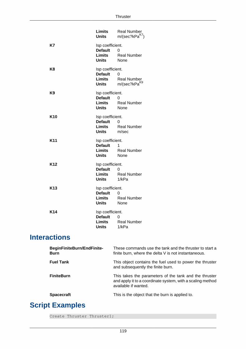
Thruster
119
Limits Real NumberUnits m/(sec?kPaK7)
K7 Isp coefficient.Default 0Limits Real NumberUnits None
K8 Isp coefficient.Default 0Limits Real NumberUnits m/(sec?kPaK9
K9 Isp coefficient.Default 0Limits Real NumberUnits None
K10 Isp coefficient.Default 0Limits Real NumberUnits m/sec
K11 Isp coefficient.Default 1Limits Real NumberUnits None
K12 Isp coefficient.Default 0Limits Real NumberUnits 1/kPa
K13 Isp coefficient.Default 0Limits Real NumberUnits None
K14 Isp coefficient.Default 0Limits Real NumberUnits 1/kPa
InteractionsBeginFiniteBurn/EndFinite-Burn
These commands use the tank and the thruster to start afinite burn, where the delta V is not instantaneous.
Fuel Tank This object contains the fuel used to power the thrusterand subsequently the finite burn.
FiniteBurn This takes the parameters of the tank and the thrusterand apply it to a coordinate system, with a scaling methodavailable if wanted.
Spacecraft This is the object that the burn is applied to.
Script ExamplesCreate Thruster Thruster1;
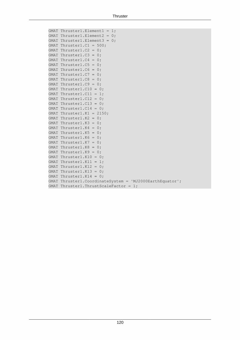
Thruster
120
GMAT Thruster1.Element1 = 1;GMAT Thruster1.Element2 = 0;GMAT Thruster1.Element3 = 0;GMAT Thruster1.C1 = 500;GMAT Thruster1.C2 = 0;GMAT Thruster1.C3 = 0;GMAT Thruster1.C4 = 0;GMAT Thruster1.C5 = 0;GMAT Thruster1.C6 = 0;GMAT Thruster1.C7 = 0;GMAT Thruster1.C8 = 0;GMAT Thruster1.C9 = 0;GMAT Thruster1.C10 = 0;GMAT Thruster1.C11 = 1;GMAT Thruster1.C12 = 0;GMAT Thruster1.C13 = 0;GMAT Thruster1.C14 = 0;GMAT Thruster1.K1 = 2150;GMAT Thruster1.K2 = 0;GMAT Thruster1.K3 = 0;GMAT Thruster1.K4 = 0;GMAT Thruster1.K5 = 0;GMAT Thruster1.K6 = 0;GMAT Thruster1.K7 = 0;GMAT Thruster1.K8 = 0;GMAT Thruster1.K9 = 0;GMAT Thruster1.K10 = 0;GMAT Thruster1.K11 = 1;GMAT Thruster1.K12 = 0;GMAT Thruster1.K13 = 0;GMAT Thruster1.K14 = 0;GMAT Thruster1.CoordinateSystem = 'MJ2000EarthEquator';GMAT Thruster1.ThrustScaleFactor = 1;
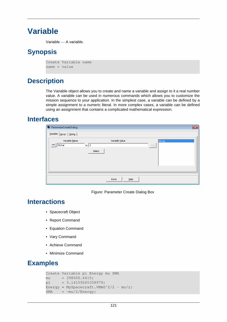
121
VariableVariable — A variable.
SynopsisCreate Variable namename = value
DescriptionThe Variable object allows you to create and name a variable and assign to it a real numbervalue. A variable can be used in numerous commands which allows you to customize themission sequence to your application. In the simplest case, a variable can be defined by asimple assignment to a numeric literal. In more complex cases, a variable can be definedusing an assignment that contains a complicated mathematical expression.
Interfaces
Figure: Parameter Create Dialog Box
Interactions• Spacecraft Object
• Report Command
• Equation Command
• Vary Command
• Achieve Command
• Minimize Command
ExamplesCreate Variable pi Energy mu SMAmu = 398600.4415;pi = 3.14159265358979;Energy = MySpacecraft.VMAG^2/2 - mu/r; SMA = -mu/2/Energy;
122
VF13adOptimizerVF13adOptimizer — Under Construction.
Synopsis Under Construction.
DescriptionUnder Construction.
FieldsField Name Description....
Type Fill This In.Default Fill This In.Limits Fill This In.Units Fill This In.
Examples
Example 10. Example Script
%
123
XYPlotXY Plot — A XY Plot.
SynopsisCreate XYPlot namename.field = value
DescriptionThe XY Plot is a graph under the Plots/Reports folder in the resource tree that plots data ontothe X and Y axes of the graph. Any two parameters can be chosen to plot from the ParameterSelect dialog box when the View radio button is clicked. The plot has the capability to beturned on and/or off throughout the mission if desirable.
InteractionsSpacecraft Spacecraft interact with an XY Plot throughout the entire mission. The
data retrieved from the spacecraft, as it carries out the command, iswhat gets plotted onto the graph.
Toggle Com-mand
A Toggle can be inserted into the mission sequence to control when theXY Plot is to plot data by subscribing it to the Toggle list. If it is necessaryto only plot data at a certain point during the mission, besides at thebeginning or end points, then two Toggle commands can be added toswitch it on and off.
FieldsIndVar The IndVar field allows the user to define the independent vari-
able for an xy-plot. Only one variable can be defined as anindependent variable. For example, the line MyXYPlot.IndVar =DefaultSC.A1ModJulian sets the independent variable to be theepoch of DefaultSC in the A1 time system and modified Julian for-mat.Default DefaultSC.A1ModJulianLimits Any user variable, array element, or spacecraft parame-
terUnits None
Add The Add field allows the user to add dependent variables toan xy-plot. All dependent variables are plotted on the y-axisvsthe independent variable defined by IndVar. To define multipledependent variables, they should be included in curly braces.For example, MyXYPlot.Add = DefaultSC.EarthMJ2000Eq.Y ,DefaultSC.EarthMJ2000Eq.Z. The GUI's Selected field is the equiv-alent of the script's Add field. In the event of no Add command or noobjects in the Selected field, GMAT should run without the XYPlotand a warning message displayed in the message window. The fol-lowing warning message is sufficient: XYPlot will be turned off. Noobject has been selected for plotting.Default DefaultSC.EarthMJ2000Eq.XLimits Any user variable, array element, or spacecraft parame-
ter
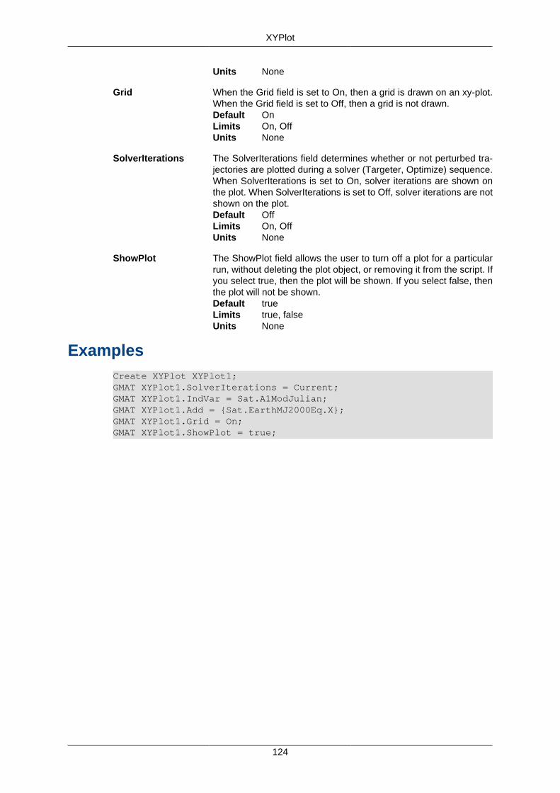
XYPlot
124
Units None
Grid When the Grid field is set to On, then a grid is drawn on an xy-plot.When the Grid field is set to Off, then a grid is not drawn.Default OnLimits On, OffUnits None
SolverIterations The SolverIterations field determines whether or not perturbed tra-jectories are plotted during a solver (Targeter, Optimize) sequence.When SolverIterations is set to On, solver iterations are shown onthe plot. When SolverIterations is set to Off, solver iterations are notshown on the plot.Default OffLimits On, OffUnits None
ShowPlot The ShowPlot field allows the user to turn off a plot for a particularrun, without deleting the plot object, or removing it from the script. Ifyou select true, then the plot will be shown. If you select false, thenthe plot will not be shown.Default trueLimits true, falseUnits None
ExamplesCreate XYPlot XYPlot1;GMAT XYPlot1.SolverIterations = Current;GMAT XYPlot1.IndVar = Sat.A1ModJulian;GMAT XYPlot1.Add = {Sat.EarthMJ2000Eq.X};GMAT XYPlot1.Grid = On;GMAT XYPlot1.ShowPlot = true;

125
Commands
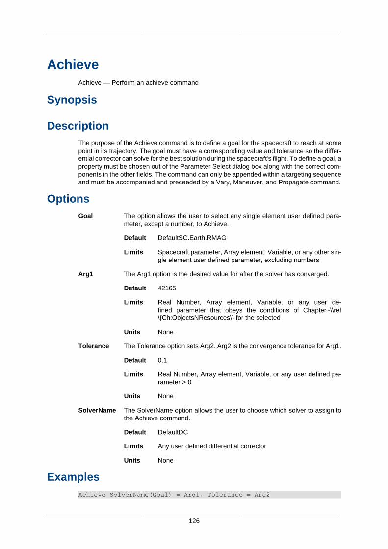
126
AchieveAchieve — Perform an achieve command
Synopsis
DescriptionThe purpose of the Achieve command is to define a goal for the spacecraft to reach at somepoint in its trajectory. The goal must have a corresponding value and tolerance so the differ-ential corrector can solve for the best solution during the spacecraft's flight. To define a goal, aproperty must be chosen out of the Parameter Select dialog box along with the correct com-ponents in the other fields. The command can only be appended within a targeting sequenceand must be accompanied and preceeded by a Vary, Maneuver, and Propagate command.
OptionsGoal The option allows the user to select any single element user defined para-
meter, except a number, to Achieve.
Default DefaultSC.Earth.RMAG
Limits Spacecraft parameter, Array element, Variable, or any other sin-gle element user defined parameter, excluding numbers
Arg1 The Arg1 option is the desired value for after the solver has converged.
Default 42165
Limits Real Number, Array element, Variable, or any user de-fined parameter that obeys the conditions of Chapter~\\ref\{Ch:ObjectsNResources\} for the selected
Units None
Tolerance The Tolerance option sets Arg2. Arg2 is the convergence tolerance for Arg1.
Default 0.1
Limits Real Number, Array element, Variable, or any user defined pa-rameter > 0
Units None
SolverName The SolverName option allows the user to choose which solver to assign tothe Achieve command.
Default DefaultDC
Limits Any user defined differential corrector
Units None
ExamplesAchieve SolverName(Goal) = Arg1, Tolerance = Arg2
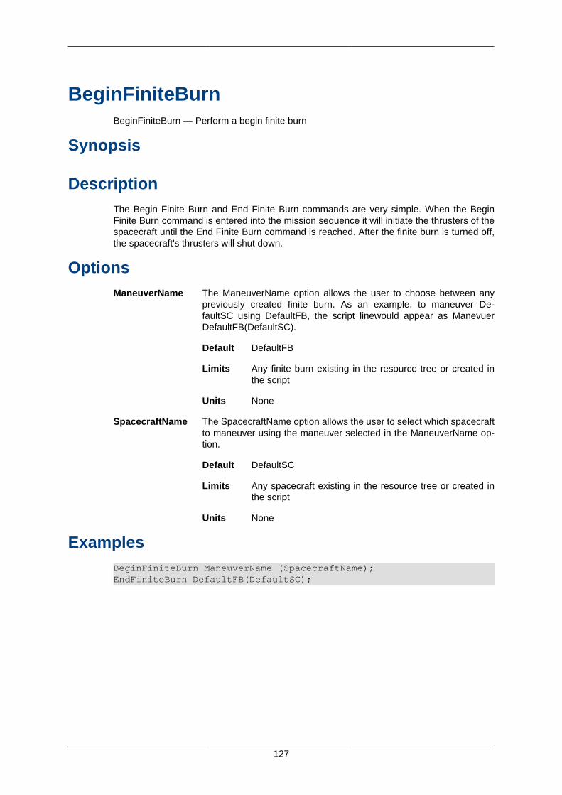
127
BeginFiniteBurnBeginFiniteBurn — Perform a begin finite burn
Synopsis
DescriptionThe Begin Finite Burn and End Finite Burn commands are very simple. When the BeginFinite Burn command is entered into the mission sequence it will initiate the thrusters of thespacecraft until the End Finite Burn command is reached. After the finite burn is turned off,the spacecraft's thrusters will shut down.
OptionsManeuverName The ManeuverName option allows the user to choose between any
previously created finite burn. As an example, to maneuver De-faultSC using DefaultFB, the script linewould appear as ManevuerDefaultFB(DefaultSC).
Default DefaultFB
Limits Any finite burn existing in the resource tree or created inthe script
Units None
SpacecraftName The SpacecraftName option allows the user to select which spacecraftto maneuver using the maneuver selected in the ManeuverName op-tion.
Default DefaultSC
Limits Any spacecraft existing in the resource tree or created inthe script
Units None
ExamplesBeginFiniteBurn ManeuverName (SpacecraftName); EndFiniteBurn DefaultFB(DefaultSC);
128
BeginMissionSequenceBeginMissionSequence — Under construction.
SynopsisUnder construction.
Under construction.Under construction.
Examples
Script Syntax
Under construction.
Script Examples
Under construction.
129
CallFunctionCall Function — Perform a call function
Synopsis
DefinitionGMAT functions are very useful and work nearly the same as they do in most programminglanguages. They may be invoked using the Call Function command covered here.
OptionsOutputList The OutputList option allows the user to set the output of Function to a user
defined parameter.
Default None
Limits Variables, Arrays, S/C, Paramters, any other user-defined para-meters, or blank. Multiple outputs must be expressed in a com-ma delimited list format
Units None
InputList The InputList option allows the user to set the input of Function to a userdefined parameter.
Default None
Limits Variables, Arrays, S/C, Paramters, any other user-defined para-meters, or blank. Multiple inputs must be expressed in a commadelimited list format.
Units None
Function The Function option allows the user to set the function that will be called ina specific location of the mission sequence. The function has to be definedbefore it can be used in the CallFunction Command.
Default None
Limits GMAT of Matlab Function
Units None
Examples
Script Syntax
%Function call with Inputs and OutputsGMAT [OutputList] = Function(InputList)
%Function call with Outputs onlyGMAT [OutputList] = Function
CallFunction
130
%Function call with Inputs onlyGMAT Function(InputList)
Function call with no Inputs or OutputsGMAT Function
Script Examples
% Matlab function call without inputs or outputs
% Syntax 1GMAT clearAll
% Syntax 2GMAT [ ] = clearAll( )
131
ElseElse — Perform an else statement
Synopsis
DescriptionIf-Else statements in GMAT work as they do in other programming languages, especiallyMatlab. The Else command adds another dimension to an If statement. You use an Elsestatement when you want something to happen when the conditions of an If statement are notmet. For example, an If statement who's condition is "x < 5" will only execute the script withinits scope when x is indeed less than 5. GMAT would otherwise pass over the If statement'sassociated script and continue. However, having an Else statement after the If will ensure thatthe lines of script within the scope of that Else are executed when x is equal to 5 or greater.
Examples
Script Syntax
If <logical expression>; <Statements>;Else; <Statements>;EndIf;
Script Examples
If DefaultSC.ElapsedDays < 1; Propagate DefaultProp( DefaultSC , { DefaultSC.ElapsedDays = 0.01 });Else; Propagate DefaultProp( DefaultSC , { DefaultSC.ElapsedDays = 0.2 });EndIf;
132
EndFiniteBurnEndFiniteBurn — Under construction.
SynopsisUnder construction.
Under construction.Under construction.
Examples
Script Syntax
Under construction.
Script Examples
Under construction.
133
EquationEquation — Perform an equation command
Synopsis
DescriptionThe Equation command uses the Equation to make one variable equal to some combinationof previously defined variables and values. It is highly useful for storing values so that theyaren't lost. Additionally, it is very useful for advanced commands.
OptionsArg1 The Arg1 option allows the user to set Arg1 to Arg2.
Default None
Limits Spacecraft Parameter, Array element, Variable, or any other single ele-ment user defined parameter
Units None
Arg2 The Arg2 option allows the user to define Arg1.
Default None
Limits Spacecraft Parameter, Array element, Variable, any other single elementuser defined parameter, or a combination of the aforementioned para-meters using math operators
Units None
Examples
Script Syntax
GMAT Arg1 = Arg2;
Script Examples
% Setting a variable to a number GMAT testVar = 24; % Setting a variable to the value of a math statement GMAT testVar = (testVar2 + 50)/2;
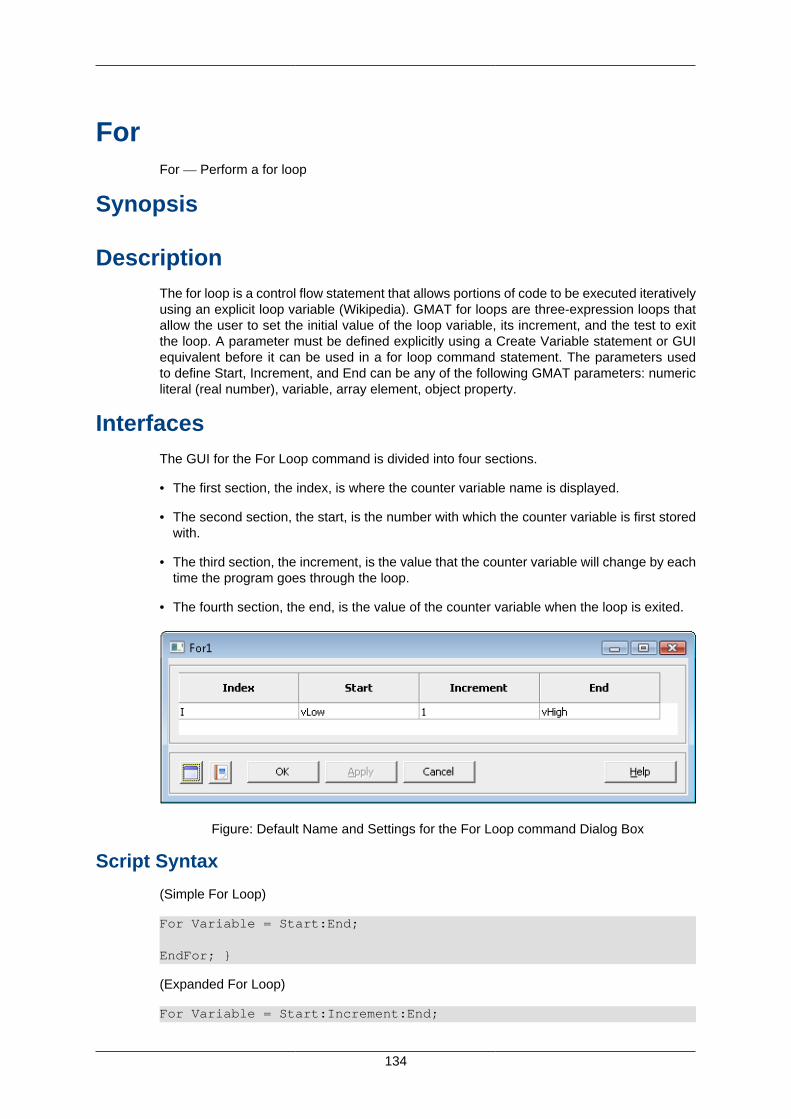
134
ForFor — Perform a for loop
Synopsis
DescriptionThe for loop is a control flow statement that allows portions of code to be executed iterativelyusing an explicit loop variable (Wikipedia). GMAT for loops are three-expression loops thatallow the user to set the initial value of the loop variable, its increment, and the test to exitthe loop. A parameter must be defined explicitly using a Create Variable statement or GUIequivalent before it can be used in a for loop command statement. The parameters usedto define Start, Increment, and End can be any of the following GMAT parameters: numericliteral (real number), variable, array element, object property.
InterfacesThe GUI for the For Loop command is divided into four sections.
• The first section, the index, is where the counter variable name is displayed.
• The second section, the start, is the number with which the counter variable is first storedwith.
• The third section, the increment, is the value that the counter variable will change by eachtime the program goes through the loop.
• The fourth section, the end, is the value of the counter variable when the loop is exited.
Figure: Default Name and Settings for the For Loop command Dialog Box
Script Syntax
(Simple For Loop)
For Variable = Start:End;
EndFor; }
(Expanded For Loop)
For Variable = Start:Increment:End;
For
135
EndFor;
Script Examples
% Output the value of the For loop Variable to a fileFor I = 1:1:10;GMAT testVar = I;Report DefaultReportFile I;EndFor;
OptionsVariable The Variable field allows the user to define the variable that to be incremented
during the loop process.
Default None
Limits Variable
Units None
Start The Start option allows the user to set the starting value of the For Loop.
Default 1
Limits Real Number, Array element, Variable, or any user defined para-meter
Units None
Increment The Increment option allows the user to set the increment value of the ForLoop. When the increment value is not included in a for loop statement, thedefault value is used.
Default 1
Limits Real Number, Array element, Variable, or any user defined para-meter
Units None
End The End option allows the user to set the ending value of the For Loop.
Default 10
Limits Real Number, Array, Variable, or any user defined parameter
Units None
For Loop BehaviorWhen the Increment option is left out of the script syntax the default value is used. If anIncrement value of 0 is used, the For Loop should not execute but GMAT should continueto run. If End>Start and Increment<0, then the For Loop should not execute. If Start>Endand Increment>0, then the For Loop should not execute. End can be equal to Start, but theFor Loop will not execute.
136
IfIf — Perform an if command
Synopsis
Description
The If command gives you the ability to use a logical statement within GMAT. At some pointduring a mission sequence, when a particular command should only be executed when acertain condition is met, use of the If command is recommended. The If command also givesyou the ability to make a command's execution reliant upon multiple conditions.
Options
<If Command> Arg1 and Arg2 can be any of the following: Real Number, Array element,Variable, Spacecraft Parameter or any other user defined parameter.
Default DefaultSC.ElapsedDays < 1.0
Limits Arg1 < Arg2 and < can be >, <, >=, <=, ==, ~126~=
Units None
<Statements> Default None
Limits Any script line that can be in the mission sequence
Units None
| The | option allows the user to set an OR operator in between <logicalexpression>s.
Default None
Limits None
Units None
& The & option allows the user to set an AND operator in between <logicalexpression>s
Default None
Limits None
Units None
Examples
Using the If command in the script is quite simple. If you have ever programmed before in thehigher level languages such as C, Matlab, or Java, GMAT will be very familiar. The statementreads like you see it basically: If the given statement after the 'If' is true, then execute thestatement(s) following until the 'EndIf' is reached.
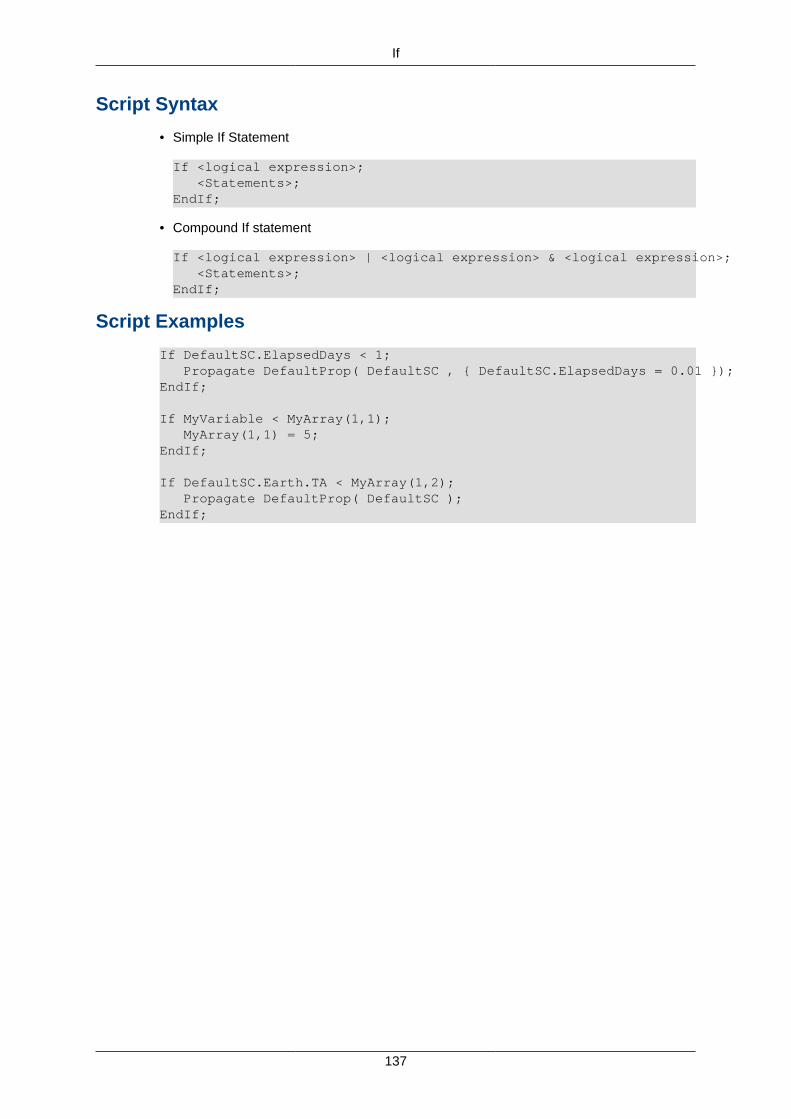
If
137
Script Syntax
• Simple If Statement
If <logical expression>; <Statements>;EndIf;
• Compound If statement
If <logical expression> | <logical expression> & <logical expression>; <Statements>;EndIf;
Script Examples
If DefaultSC.ElapsedDays < 1; Propagate DefaultProp( DefaultSC , { DefaultSC.ElapsedDays = 0.01 });EndIf;
If MyVariable < MyArray(1,1); MyArray(1,1) = 5;EndIf;
If DefaultSC.Earth.TA < MyArray(1,2); Propagate DefaultProp( DefaultSC );EndIf;
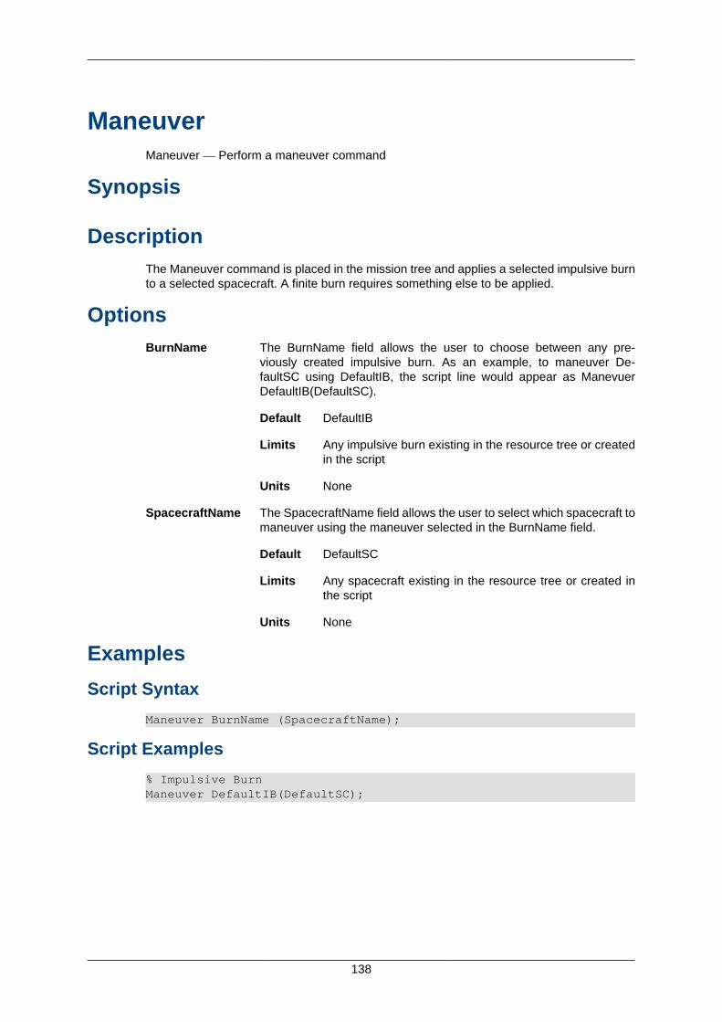
138
ManeuverManeuver — Perform a maneuver command
Synopsis
DescriptionThe Maneuver command is placed in the mission tree and applies a selected impulsive burnto a selected spacecraft. A finite burn requires something else to be applied.
OptionsBurnName The BurnName field allows the user to choose between any pre-
viously created impulsive burn. As an example, to maneuver De-faultSC using DefaultIB, the script line would appear as ManevuerDefaultIB(DefaultSC).
Default DefaultIB
Limits Any impulsive burn existing in the resource tree or createdin the script
Units None
SpacecraftName The SpacecraftName field allows the user to select which spacecraft tomaneuver using the maneuver selected in the BurnName field.
Default DefaultSC
Limits Any spacecraft existing in the resource tree or created inthe script
Units None
Examples
Script Syntax
Maneuver BurnName (SpacecraftName);
Script Examples
% Impulsive BurnManeuver DefaultIB(DefaultSC);
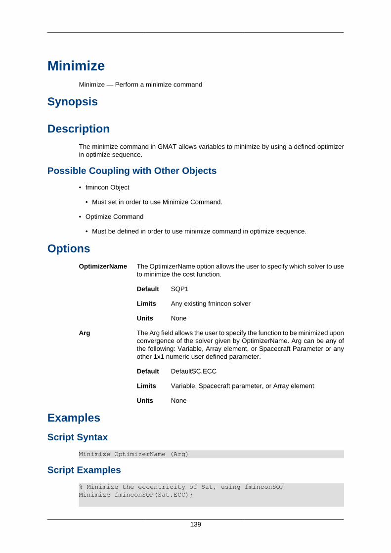
139
MinimizeMinimize — Perform a minimize command
Synopsis
DescriptionThe minimize command in GMAT allows variables to minimize by using a defined optimizerin optimize sequence.
Possible Coupling with Other Objects
• fmincon Object
• Must set in order to use Minimize Command.
• Optimize Command
• Must be defined in order to use minimize command in optimize sequence.
OptionsOptimizerName The OptimizerName option allows the user to specify which solver to use
to minimize the cost function.
Default SQP1
Limits Any existing fmincon solver
Units None
Arg The Arg field allows the user to specify the function to be minimized uponconvergence of the solver given by OptimizerName. Arg can be any ofthe following: Variable, Array element, or Spacecraft Parameter or anyother 1x1 numeric user defined parameter.
Default DefaultSC.ECC
Limits Variable, Spacecraft parameter, or Array element
Units None
Examples
Script Syntax
Minimize OptimizerName (Arg)
Script Examples
% Minimize the eccentricity of Sat, using fminconSQPMinimize fminconSQP(Sat.ECC);

Minimize
140
% Minimize the Variable DeltaV, using fminconSQPMinimize fminconSQP(DeltaV);
% Minimize the first component of MyArray, using fminconSQPMinimize fminconSQP(MyArray(1,1));
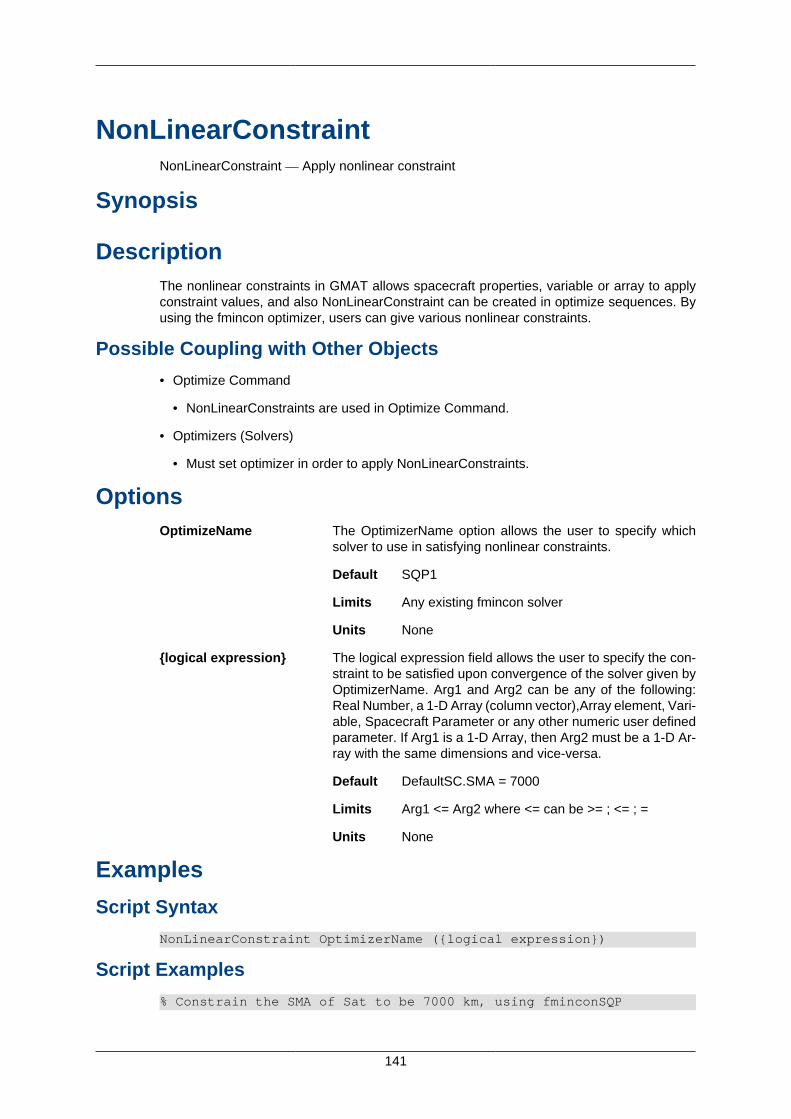
141
NonLinearConstraintNonLinearConstraint — Apply nonlinear constraint
Synopsis
DescriptionThe nonlinear constraints in GMAT allows spacecraft properties, variable or array to applyconstraint values, and also NonLinearConstraint can be created in optimize sequences. Byusing the fmincon optimizer, users can give various nonlinear constraints.
Possible Coupling with Other Objects
• Optimize Command
• NonLinearConstraints are used in Optimize Command.
• Optimizers (Solvers)
• Must set optimizer in order to apply NonLinearConstraints.
OptionsOptimizeName The OptimizerName option allows the user to specify which
solver to use in satisfying nonlinear constraints.
Default SQP1
Limits Any existing fmincon solver
Units None
{logical expression} The logical expression field allows the user to specify the con-straint to be satisfied upon convergence of the solver given byOptimizerName. Arg1 and Arg2 can be any of the following:Real Number, a 1-D Array (column vector),Array element, Vari-able, Spacecraft Parameter or any other numeric user definedparameter. If Arg1 is a 1-D Array, then Arg2 must be a 1-D Ar-ray with the same dimensions and vice-versa.
Default DefaultSC.SMA = 7000
Limits Arg1 <= Arg2 where <= can be >= ; <= ; =
Units None
Examples
Script Syntax
NonLinearConstraint OptimizerName ({logical expression})
Script Examples
% Constrain the SMA of Sat to be 7000 km, using fminconSQP
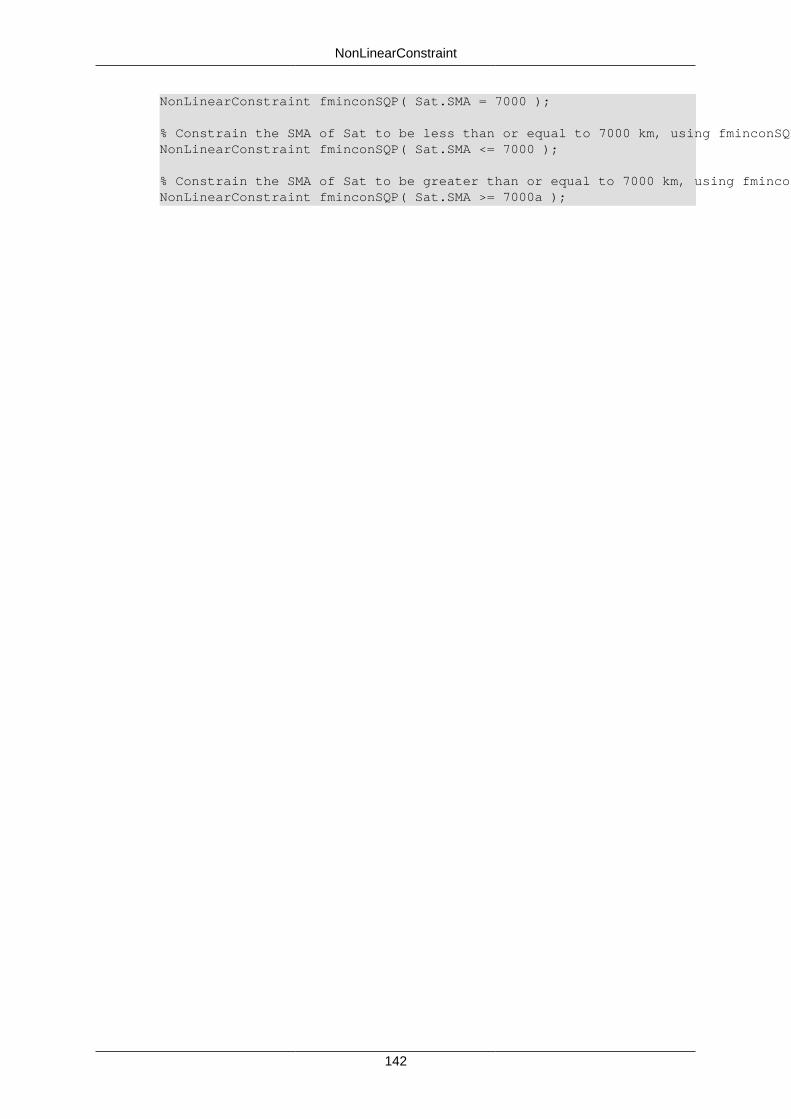
NonLinearConstraint
142
NonLinearConstraint fminconSQP( Sat.SMA = 7000 );
% Constrain the SMA of Sat to be less than or equal to 7000 km, using fminconSQPNonLinearConstraint fminconSQP( Sat.SMA <= 7000 );
% Constrain the SMA of Sat to be greater than or equal to 7000 km, using fminconSQPNonLinearConstraint fminconSQP( Sat.SMA >= 7000a );
143
OptimizeOptimize — Perform an optimize command
Synopsis
DescriptionThe optimize command in GMAT allows variables to optimize by using a solver fminconobject.
Possible Coupling with Other Objects
• fmincon Object
• Must set in order to use Optimize Command.
• Minimize
• Must be defined if you would like to minimize variable in an optimize sequence.
• Vary
• NonLinearConstraint
OptionsSolverName The SolverName field allows the user to choose between any previously
created optimizer for use in an optimization sequence. For example, tobegin a optimization sequence using DefaultSQP, the script is OptimizeDefaultSQP.
Default DefaultSQP
Limits Any existing optimizer
Units None
<Statements>Default None
Limits Any non-targeter and non-optimizer command lines used inthe mission sequence, as well as the optimizer dependentcommand lines Vary, NonLinearConstraint, and Minimize.
Units None
Examples
Script Syntax
Optimize SolverName; <Statements>;EndOptimize;
Optimize
144
Script Examples
% Beginning and ending syntax for the Optimize commandOptimize DefaultDC;
EndOptimize;
145
PenUpPenUp — Under construction.
SynopsisUnder construction.
Under construction.Under construction.
Examples
Script Syntax
Under construction.
Script Examples
Under construction.
146
PenDownPenDown — Under construction.
SynopsisUnder construction.
Under construction.Under construction.
Examples
Script Syntax
Under construction.
Script Examples
Under construction.
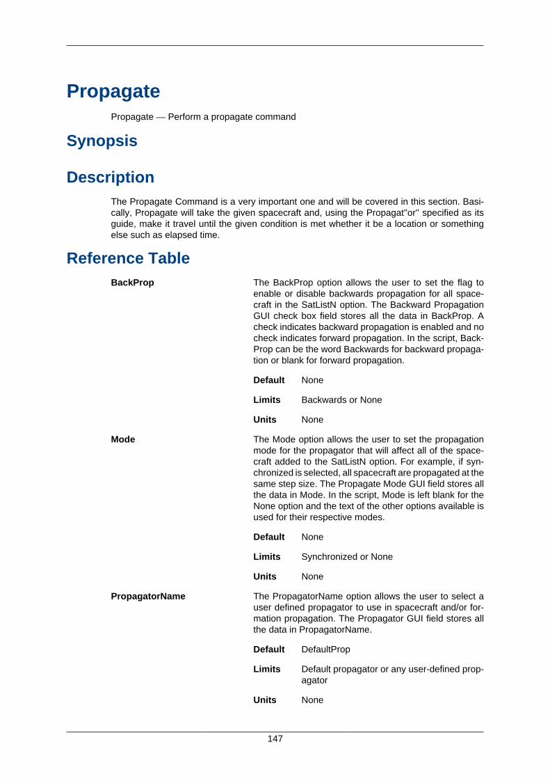
147
PropagatePropagate — Perform a propagate command
Synopsis
DescriptionThe Propagate Command is a very important one and will be covered in this section. Basi-cally, Propagate will take the given spacecraft and, using the Propagat''or'' specified as itsguide, make it travel until the given condition is met whether it be a location or somethingelse such as elapsed time.
Reference TableBackProp The BackProp option allows the user to set the flag to
enable or disable backwards propagation for all space-craft in the SatListN option. The Backward PropagationGUI check box field stores all the data in BackProp. Acheck indicates backward propagation is enabled and nocheck indicates forward propagation. In the script, Back-Prop can be the word Backwards for backward propaga-tion or blank for forward propagation.
Default None
Limits Backwards or None
Units None
Mode The Mode option allows the user to set the propagationmode for the propagator that will affect all of the space-craft added to the SatListN option. For example, if syn-chronized is selected, all spacecraft are propagated at thesame step size. The Propagate Mode GUI field stores allthe data in Mode. In the script, Mode is left blank for theNone option and the text of the other options available isused for their respective modes.
Default None
Limits Synchronized or None
Units None
PropagatorName The PropagatorName option allows the user to select auser defined propagator to use in spacecraft and/or for-mation propagation. The Propagator GUI field stores allthe data in PropagatorName.
Default DefaultProp
Limits Default propagator or any user-defined prop-agator
Units None
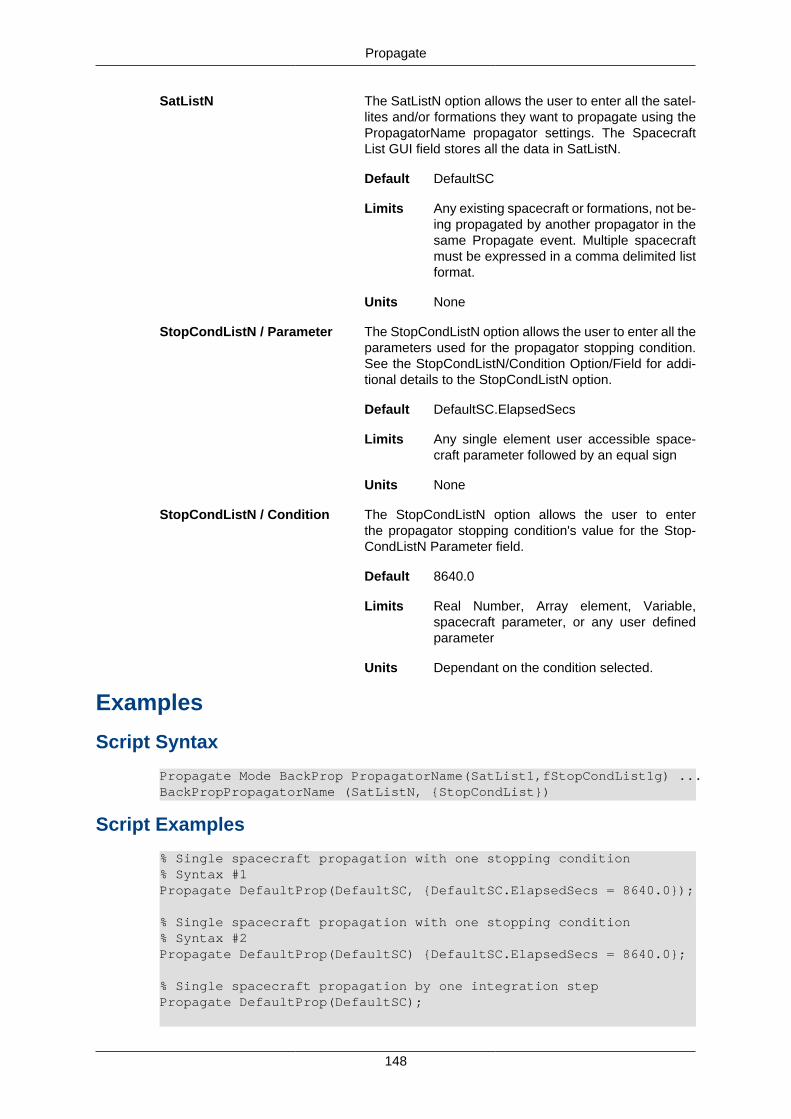
Propagate
148
SatListN The SatListN option allows the user to enter all the satel-lites and/or formations they want to propagate using thePropagatorName propagator settings. The SpacecraftList GUI field stores all the data in SatListN.
Default DefaultSC
Limits Any existing spacecraft or formations, not be-ing propagated by another propagator in thesame Propagate event. Multiple spacecraftmust be expressed in a comma delimited listformat.
Units None
StopCondListN / Parameter The StopCondListN option allows the user to enter all theparameters used for the propagator stopping condition.See the StopCondListN/Condition Option/Field for addi-tional details to the StopCondListN option.
Default DefaultSC.ElapsedSecs
Limits Any single element user accessible space-craft parameter followed by an equal sign
Units None
StopCondListN / Condition The StopCondListN option allows the user to enterthe propagator stopping condition's value for the Stop-CondListN Parameter field.
Default 8640.0
Limits Real Number, Array element, Variable,spacecraft parameter, or any user definedparameter
Units Dependant on the condition selected.
Examples
Script Syntax
Propagate Mode BackProp PropagatorName(SatList1,fStopCondList1g) ...BackPropPropagatorName (SatListN, {StopCondList})
Script Examples
% Single spacecraft propagation with one stopping condition% Syntax #1Propagate DefaultProp(DefaultSC, {DefaultSC.ElapsedSecs = 8640.0});
% Single spacecraft propagation with one stopping condition% Syntax #2Propagate DefaultProp(DefaultSC) {DefaultSC.ElapsedSecs = 8640.0};
% Single spacecraft propagation by one integration stepPropagate DefaultProp(DefaultSC);
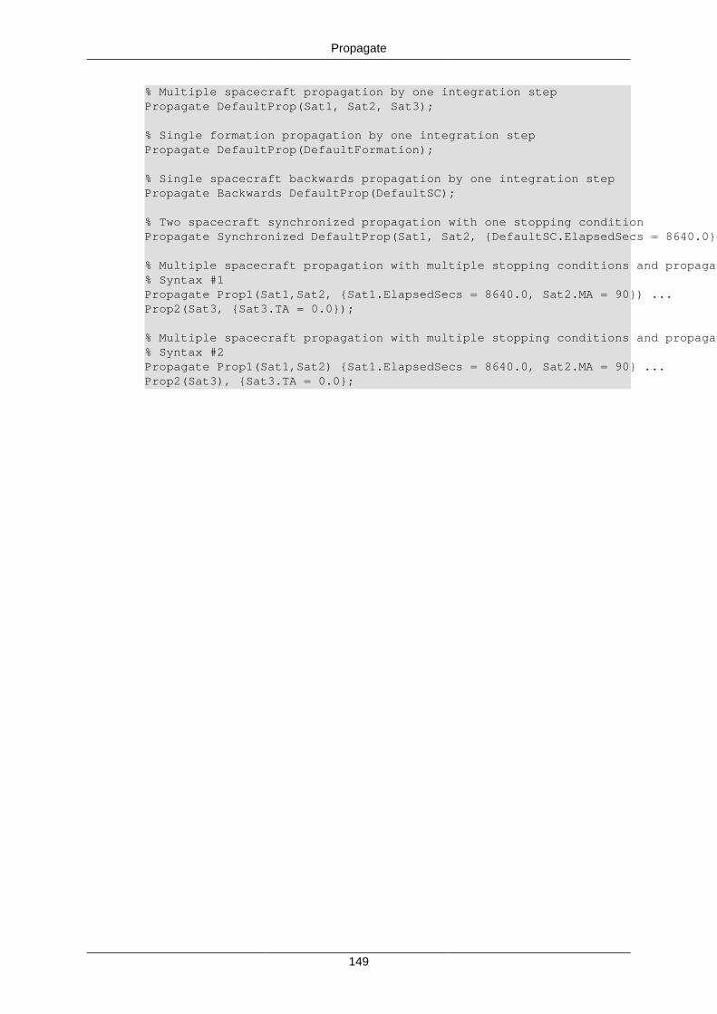
Propagate
149
% Multiple spacecraft propagation by one integration stepPropagate DefaultProp(Sat1, Sat2, Sat3);
% Single formation propagation by one integration stepPropagate DefaultProp(DefaultFormation);
% Single spacecraft backwards propagation by one integration stepPropagate Backwards DefaultProp(DefaultSC);
% Two spacecraft synchronized propagation with one stopping conditionPropagate Synchronized DefaultProp(Sat1, Sat2, {DefaultSC.ElapsedSecs = 8640.0});
% Multiple spacecraft propagation with multiple stopping conditions and propagation settings% Syntax #1Propagate Prop1(Sat1,Sat2, {Sat1.ElapsedSecs = 8640.0, Sat2.MA = 90}) ...Prop2(Sat3, {Sat3.TA = 0.0});
% Multiple spacecraft propagation with multiple stopping conditions and propagation settings% Syntax #2Propagate Prop1(Sat1,Sat2) {Sat1.ElapsedSecs = 8640.0, Sat2.MA = 90} ...Prop2(Sat3), {Sat3.TA = 0.0};
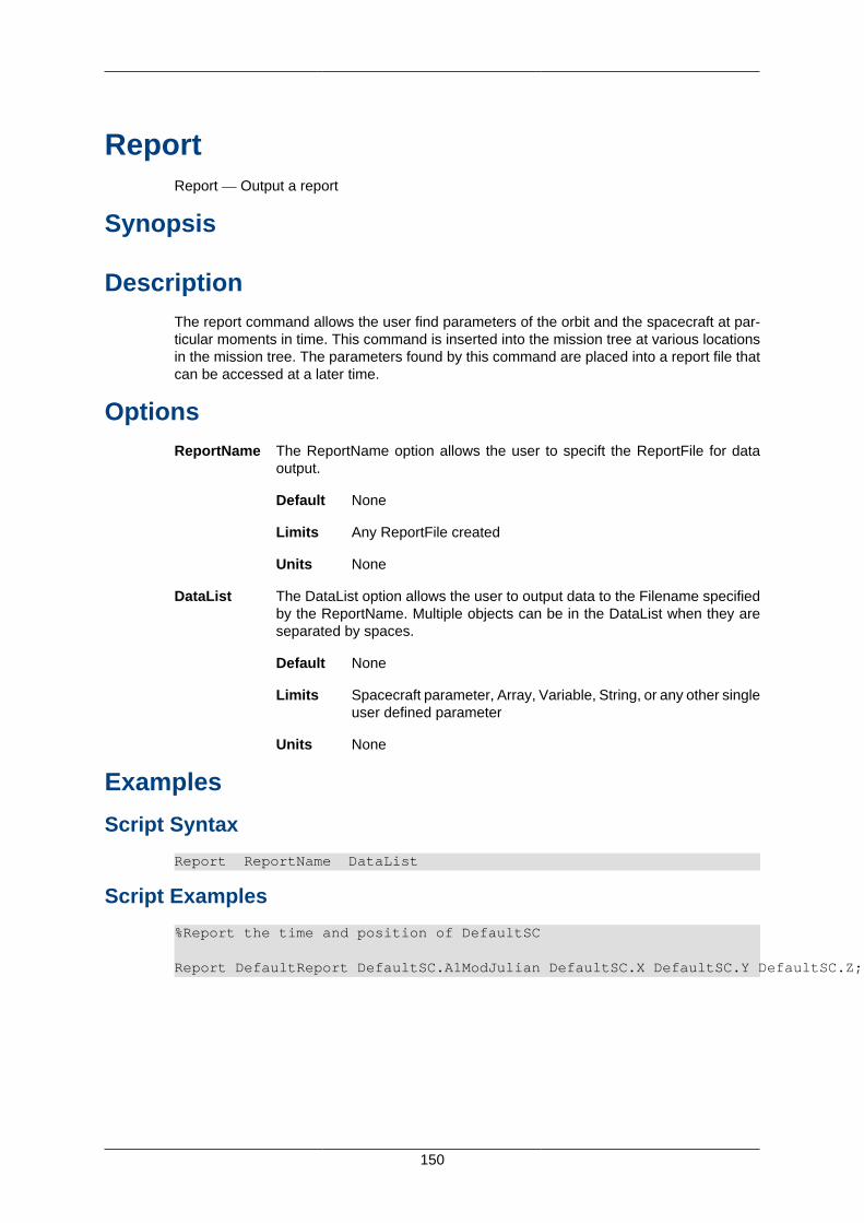
150
ReportReport — Output a report
Synopsis
DescriptionThe report command allows the user find parameters of the orbit and the spacecraft at par-ticular moments in time. This command is inserted into the mission tree at various locationsin the mission tree. The parameters found by this command are placed into a report file thatcan be accessed at a later time.
OptionsReportName The ReportName option allows the user to specift the ReportFile for data
output.
Default None
Limits Any ReportFile created
Units None
DataList The DataList option allows the user to output data to the Filename specifiedby the ReportName. Multiple objects can be in the DataList when they areseparated by spaces.
Default None
Limits Spacecraft parameter, Array, Variable, String, or any other singleuser defined parameter
Units None
Examples
Script Syntax
Report ReportName DataList
Script Examples
%Report the time and position of DefaultSC
Report DefaultReport DefaultSC.A1ModJulian DefaultSC.X DefaultSC.Y DefaultSC.Z;
151
SaveSave — Under construction.
SynopsisUnder construction.
Under construction.Under construction.
Examples
Script Syntax
Under construction.
Script Examples
Under construction.
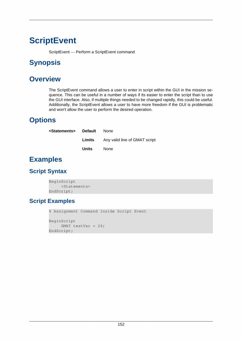
152
ScriptEventScriptEvent — Perform a ScriptEvent command
Synopsis
OverviewThe ScriptEvent command allows a user to enter in script within the GUI in the mission se-quence. This can be useful in a number of ways if its easier to enter the script than to usethe GUI interface. Also, if multiple things needed to be changed rapidly, this could be useful.Additionally, the ScriptEvent allows a user to have more freedom if the GUI is problematicand won't allow the user to perform the desired operation.
Options<Statements> Default None
Limits Any valid line of GMAT script
Units None
Examples
Script Syntax
BeginScript <Statements>EndScript;
Script Examples
% Assignment Command inside Script Event
BeginScript GMAT testVar = 24;EndScript;
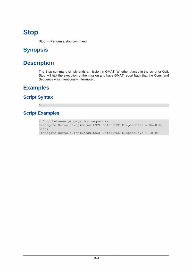
153
StopStop — Perform a stop command
Synopsis
DescriptionThe Stop command simply ends a mission in GMAT. Whether placed in the script or GUI,Stop will halt the execution of the mission and have GMAT report back that the CommandSequence was intentionally interrupted.
Examples
Script Syntax
Stop
Script Examples
% Stop between propagation sequencesPropagate DefaultProp(DefaultSC) DefaultSC.ElapsedSecs = 8640.0;Stop;Propagate DefaultProp(DefaultSC) DefaultSC.ElapsedDays = 10.0;
154
TargetTarget — Perform a targeting sequence
SynopsisTarget SolverName(options) Vary SolverName(Vary arguments); Achieve SolverName(Achieve arguments); [Other Commands;] …EndTarget
DescriptionWhen building a mission, the targeting sequence is one of the most useful tools you haveat your disposal. It allows you to use the power of a differential corrector to find solutions tocomplex two and three-body problems with a limited number of known values and severalvariables. Target is the base command that is appended with more commands such as Vary,Maneuver, Propagate, and Achieve in order to meet your goals. This makes it the first partof the sequence to be put into the Mission tree.
ArgumentsSolverName The SolverName option allows the user to choose between any previously
created differential correctors for use in a targeting sequence. For example,to begin a targeting sequence using DefaultDC, the script is Target Default-DC.
Type DifferentialCorrector
OptionsSolveMode Tells the targeter state machine how to manage the targeter loop. When run-
ning in the RunInitialGuess mode, the target loop is executed one time usingthe initial values of the targeter variables. No targeting is performed. Whenrunning in Solve mode, the targeter searches for a solution satisfying the tar-geter goals.
Type Enumeration
Values • Solve (default)
• RunInitialGuess
ExitMode Tells the Mission Control Sequence how to proceed after the targeter loop hasfinished running. When running in DiscardAndContinue mode, subsequentcalls to the same targeter loop will reset the variables to their initial values. Ifrunning in SaveAndContinue mode, the targeter variables used on a subse-quent run start with the values obtained the last time the targeter loop was run.In Stop mode, the mission run halts when the targeter loop completes its work.
Type Enumeration
Values • DiscardAndContinue (default)
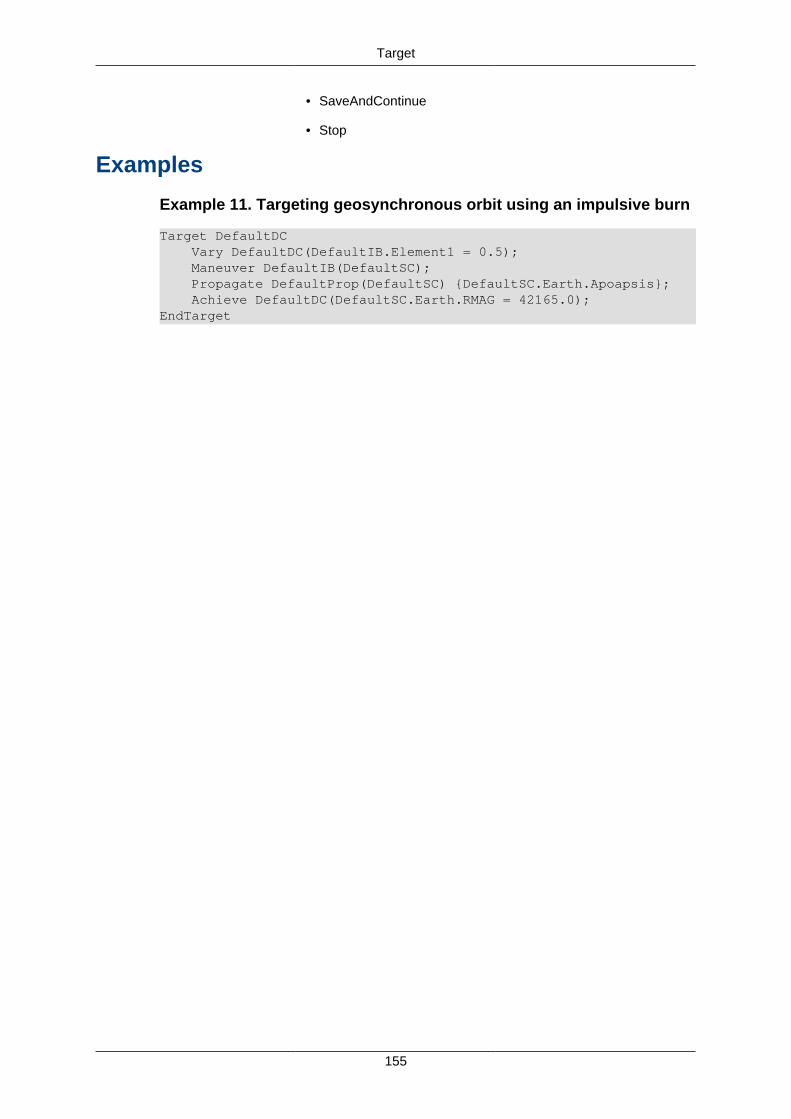
Target
155
• SaveAndContinue
• Stop
Examples
Example 11. Targeting geosynchronous orbit using an impulsive burn
Target DefaultDC Vary DefaultDC(DefaultIB.Element1 = 0.5); Maneuver DefaultIB(DefaultSC); Propagate DefaultProp(DefaultSC) {DefaultSC.Earth.Apoapsis}; Achieve DefaultDC(DefaultSC.Earth.RMAG = 42165.0);EndTarget
156
ToggleToggle — Perform a toggle command
Synopsis
DescriptionThe Toggle command is useful in turning on/off certain plots so that they do not becomeunintelligible. They are particularly useful if a mission requires multiple sequences to fine-tunethe answer. If this is the case, it might be better to turn off a plot until the final or second-to-last sequence so that the rougher sequences don't obstruct the view of what is going on inthe finesse sequences.
OptionsOutputNames The Toggle option allows the user to assign the Plot/Report(s) to be toggled.
When more than one Plot/Report is being toggled they need to be separatedby a space.
Default DefaultOpenGL
Limits Any OpenGL, Report, XYplot, or any other Plot/Report type
Units None
Arg The Arg option allows the user to turn off or on the data output to a Plot/Report.
Default On
Limits On or Off
Units None
Exmaples
Script Syntax
Toggle OutputNames Arg
Script Examples
% Turn off Report file for the first day of propagationToggle ReportFile1 OffPropagate DefaultProp(DefaultSC, {DefaultSC.ElapsedDays = 1});Toggle ReportFile1 OnPropagate DefaultProp(DefaultSC, {DefaultSC.ElapsedDays = 1});
% Turn off XYPlot and Report file for the first day of propagation Toggle XYPlot1 ReportFile1 OffPropagate DefaultProp(DefaultSC, {DefaultSC.ElapsedDays = 1});
Toggle XYPlot1 ReportFile1 On

Toggle
157
Propagate DefaultProp(DefaultSC, {DefaultSC.ElapsedDays = 1})
158
VaryVary — Perform a vary command
Synopsis
DescriptionThe Vary command is used in conjunction with the Target and Optimize Commands. TheVary command varies a particular parameter within the Target and Optimize Commands untilcertain conditions are met. It is a highly useful command for creating missions. Multiple Varycommands can be used within the same targeting or optimizing sequence.
OptionsParameters Associated with All Solvers
SolverName The SolverName option allows the user to choose which solver to assignto the vary command.
Default DefaultDC
Limits Any user defined solver
Units None
Variable The Variable option allows the user to select any single element userdefined parameter, except a number, to vary. For example, DefaultIB.V,DefaultIB.N, DefaultIB.Element1, DefaultSC.TA, Array(1,1), and Variableare all valid values. The three element burn vector or multidimensionalArrays are not valid values.
Default DefaultIB.V
Limits Spacecrafy paremeter, Array element, Variable, or any othersingle element user defined parameter, excluding numbers
Units None
InitialGuess The InitialGuess option allows the user to set the initial guess for the se-lected Variable.
Default 0.5
Limits Real Number, Array element, Variable, or any user definedparameter that obeys the conditions for the selected Variableobject
Units km/s
Lower The Lower option allows the user to set Arg3 to the lower bound of thequantity being varied.
Default 0.0
Limits Real Number, Array element, Variable, or any user definedparameter (Upper > Lower )
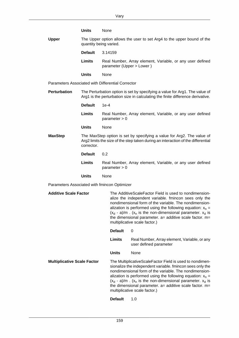
Vary
159
Units None
Upper The Upper option allows the user to set Arg4 to the upper bound of thequantity being varied.
Default 3.14159
Limits Real Number, Array element, Variable, or any user definedparameter (Upper > Lower )
Units None
Parameters Associated with Differential Corrector
Perturbation The Perturbation option is set by specifying a value for Arg1. The value ofArg1 is the perturbation size in calculating the finite difference derivative.
Default 1e-4
Limits Real Number, Array element, Variable, or any user definedparameter > 0
Units None
MaxStep The MaxStep option is set by specifying a value for Arg2. The value ofArg2 limits the size of the step taken during an interaction of the differentialcorrector.
Default 0.2
Limits Real Number, Array element, Variable, or any user definedparameter > 0
Units None
Parameters Associated with fmincon Optimizer
Additive Scale Factor The AdditiveScaleFactor Field is used to nondimension-alize the independent variable. fmincon sees only thenondimensional form of the variable. The nondimension-alization is performed using the following equation: xn =(xd - a)/m . (xn is the non-dimensional parameter. xd isthe dimensional parameter. a= additive scale factor. m=multiplicative scale factor.)
Default 0
Limits Real Number, Array element, Variable, or anyuser defined parameter
Units None
Multiplicative Scale Factor The MultiplicativeScaleFactor Field is used to nondimen-sionalize the independent variable. fmincon sees only thenondimensional form of the variable. The nondimension-alization is performed using the following equation: xn =(xd - a)/m . (xn is the non-dimensional parameter. xd isthe dimensional parameter. a= additive scale factor. m=multiplicative scale factor.)
Default 1.0
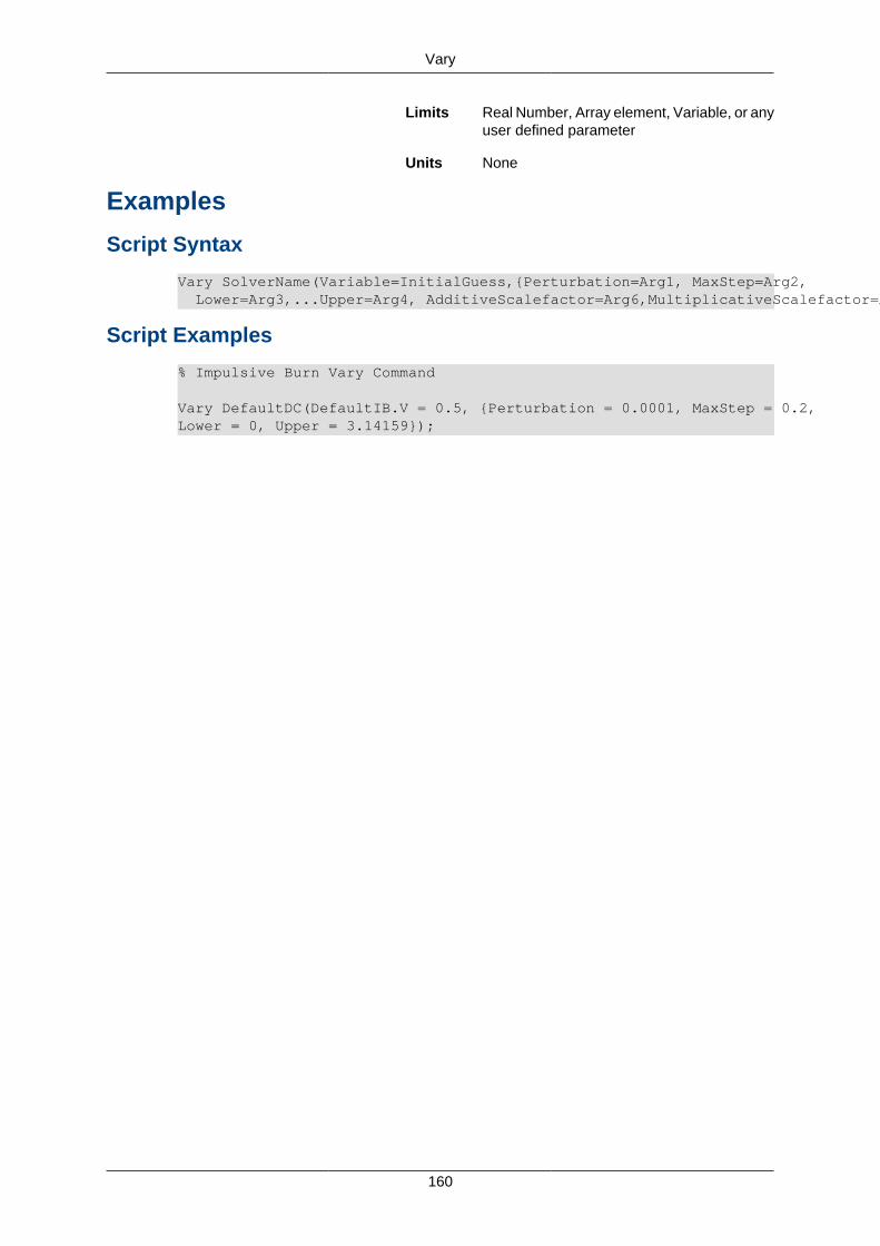
Vary
160
Limits Real Number, Array element, Variable, or anyuser defined parameter
Units None
Examples
Script Syntax
Vary SolverName(Variable=InitialGuess,{Perturbation=Arg1, MaxStep=Arg2, Lower=Arg3,...Upper=Arg4, AdditiveScalefactor=Arg6,MultiplicativeScalefactor=Arg6})
Script Examples
% Impulsive Burn Vary Command
Vary DefaultDC(DefaultIB.V = 0.5, {Perturbation = 0.0001, MaxStep = 0.2, Lower = 0, Upper = 3.14159});
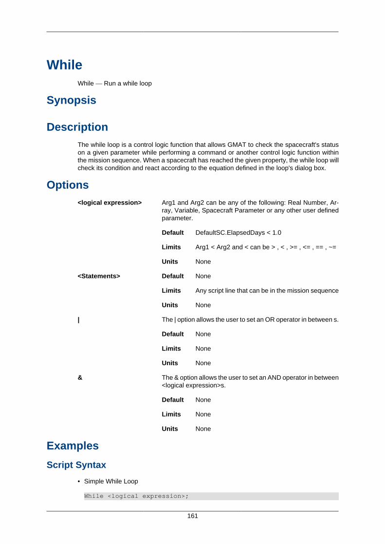
161
WhileWhile — Run a while loop
Synopsis
DescriptionThe while loop is a control logic function that allows GMAT to check the spacecraft's statuson a given parameter while performing a command or another control logic function withinthe mission sequence. When a spacecraft has reached the given property, the while loop willcheck its condition and react according to the equation defined in the loop's dialog box.
Options<logical expression> Arg1 and Arg2 can be any of the following: Real Number, Ar-
ray, Variable, Spacecraft Parameter or any other user definedparameter.
Default DefaultSC.ElapsedDays < 1.0
Limits Arg1 < Arg2 and < can be > , < , >= , <= , == , ~=
Units None
<Statements> Default None
Limits Any script line that can be in the mission sequence
Units None
| The | option allows the user to set an OR operator in between s.
Default None
Limits None
Units None
& The & option allows the user to set an AND operator in between<logical expression>s.
Default None
Limits None
Units None
Examples
Script Syntax
• Simple While Loop
While <logical expression>;
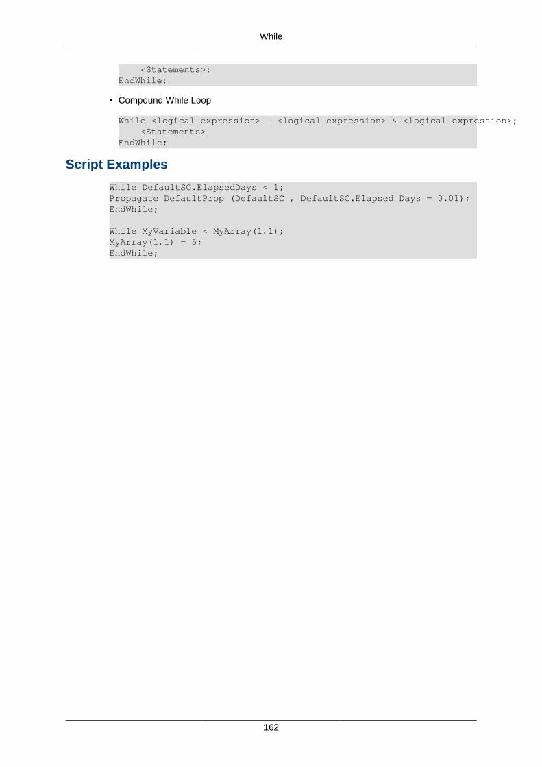
While
162
<Statements>;EndWhile;
• Compound While Loop
While <logical expression> | <logical expression> & <logical expression>; <Statements>EndWhile;
Script Examples
While DefaultSC.ElapsedDays < 1;Propagate DefaultProp (DefaultSC , DefaultSC.Elapsed Days = 0.01);EndWhile;
While MyVariable < MyArray(1,1);MyArray(1,1) = 5;EndWhile;
163
IndexAAchieve, 126Array, 70
BBaryCenter, 71BeginFiniteBurn, 127BeginMissionSequence, 128BodyNames, 71
CCallFunction, 129
EElse, 131EndFiniteBurn, 132Equation, 133
FFor, 134
IIf, 136
MManeuver, 138Minimize, 139
NNonLinearConstraint, 141
OOptimize, 143
PPenDown, 146PenUp, 145Propagate, 147
RReport, 150
SSave, 151ScriptEvent, 152Spacecraft, 107Stop, 153
TTarget, 154Toggle, 156
VVary, 158
WWhile, 161